Environmental Accounting of Financial Development and Foreign Investment: Spatial Analyses of East Asia


1
Department of Finance, College of Business Administration, Prince Sattam bin Abdulaziz University, 165, Al-Kharj 11942, Saudi Arabia
2
S&P Global Marketing Intelligence, Islamabad 44000, Pakistan
3
Department of Accounting, College of Business Administration, Prince Sattam bin Abdulaziz University, 165, Al-Kharj 11942, Saudi Arabia
*
Author to whom correspondence should be addressed.
Sustainability 2019, 11(1), 13; https://doi.org/10.3390/su11010013
Submission received: 15 November 2018
/
Revised: 11 December 2018
/
Accepted: 14 December 2018
/
Published: 20 December 2018
(This article belongs to the Section Economic and Business Aspects of Sustainability)
Abstract
:This paper aspires to examine the environmental effects of financial market development (FMD), foreign direct investment (FDI), and trade openness on the CO2 emissions per capita along with the environmental Kuznets curve (EKC) hypothesis in six East Asian countries from 1991–2014. For this purpose, spatial econometrics is applied to consider the spillover effects from neighboring countries. The results of the study corroborate the spillover effects from neighboring countries’ CO2 emissions per capita, FMD, FDI, and trade openness, and the EKC hypothesis is proven true in this region. Local FDI inflows, trade openness, and energy intensity are found to be responsible for local environmental degradation. Local FMD has an insignificant environmental effect, but neighboring countries’ FMD has contributed to the local CO2 emissions per capita. Further, positive (negative) environmental spillover effects are found from neighboring countries’ FDI (trade openness).
1. Introduction
With the world moving toward making efforts for a greener environment, the discussion about reducing CO2 emissions is inevitably brought up. Needless to say, that when it comes to constructing a greener and more sustainable environment, cutting down on CO2 emissions is one of the first things that needs to be done. On the same idea, many studies have been conducted that talk about how CO2 emissions affect the health of the ecosystem and what role macro and microeconomic factors play in determining them. Auffhammer and Carson [1] have studied CO2 emissions on a provincial level in China and mentioned that over the past five years, CO2 emissions have dramatically increased. Something unique about this study is that the existence of spatial dependency has been analyzed. Car ownership in China is about 12% than that of the U.S., but the country suffers from about the same level of road congestion, leaving many questions regarding its emissions trajectory. Another spatial analysis on China was conducted by Chen et al. [2] to explore the effects of pollution on health. After analyzing data from 116 cities in China, the existence of adverse health impact of pollution has been proven with a spatial existence, indicating that pollution affects the locals and neighbors’ health at the same time. Therefore, the spatial dependency of pollution emissions seems equally bad for the health of people and the environment.
On the discussion about CO2 emissions, the idea of the EKC should not be ignored since a large part of the discussion is based on this theory. EKC suggests that with an improvement on the overall economic health of a country, emissions first increase and then start to go down with time when the economy gains more economic growth. Many studies support this idea on several regional levels, but there is still much space to explore these claims, especially from the perspective of spatial dependency. Analyzing the concept from the spatial dependency’s dimension is essential because pollutant emissions of a country do not only play a role in its economy, they can influence other neighboring countries as well. A similar concept has been analyzed by Le and Quah [3] stating that energy usage and income seem to have a long-term association with the level of emissions in the Asia and Pacific region. However, they argued that EKC does not exist in an inverted U-shape in all countries in the selected region.
Conversely, high-income countries do have EKC in its inverted U-shaped form and with the increase in income, emissions first increase and then start to decline later. EKC could not be found in lower- or middle-income countries. It makes it essential to analyze the prevalence of EKC by incorporating spatial dependency in order to assess its role in the context. Ignoring spatial dependency, a study on the European and Central Asian region suggests that corporate governance and reforms in competition policies in the region can help to reduce the emissions rates. On the contrary, economic openness does not seem to have a stable and robust impact on emissions. Although not proven within the econometric model, the theoretical existence of spatial effects has been discussed in the study that could help to conduct the further country and region-wide analysis [4].
A spatial study on China has been presented by Guo et al. [5] where they suggested that, regardless of the strong correlation between urbanization and emissions, other factors, such as scale effect, intensive effect, and structure effect play a vital role as well. Zhao et al. [6] argue that spatial patterns could be a significant driving force for emissions and growth in a particular region and it is crucial to keep them into account while discussing the environmental profile of the region. They analyze China from a spatial perspective and mention that depending on the level of urbanization in the part of the country, emissions grow differently while industrial and environmental policies play their role in the equation as well. Ge et al. [7] have conducted a spatial study on NOx emissions of China. Through a stochastic impacts by regression on population, affluence, and technology (STIRPAT) framework, the results of the study have suggested an inverse N-shaped relationship between urbanization and NOx on a provincial level in China.
Using data from 2010–2012 from China, Pu [8] argued that there is a spatial difference between several parts of the country regarding the convergence between growth and emissions rate. While the study has landed on robust conclusions, it needs further evidence using panel data that can support this inference. Yang et al. [9] mentioned that EKC is not a standalone theory to define how well economic growth and emissions are connected. Therefore, they investigated the existence of EKC in China and mentioned that while the relation is directly affected by scale and other effects, aspects like technological advancement, environmental regulation, and industrial structure have an indirect influence on the implication of EKC. Another aspect that needs to be put into perspective here is that countries nowadays are trying to become less energy-intensive and moving towards better environmental regulation, labor redistribution, technology, and investment [10]. It is something that can have effects on a spatial level, which makes it crucial to research emissions and economic growth from a spatial dimension. Hence, this study is focused to fill the gaps in the research pool.
While many factors determine the strength of the relationship between emissions in a country and its economic growth, i.e., FDI, FMD, trade openness and energy usage be some of the major ones discussed in theory. Much recent literature talks about how the mechanism of CO2 emissions and financial development work. According to Pata [11], there is a dynamic relationship between financial development and CO2 emissions in a country. When financial development takes place in a country, urbanization seems to become improved, which leads to more use of energy. In that case, if enough alternative sources of cleaner energy are not available in a country, financial development turns out to be a source of environmental deterioration in the country. Huang and Zhao [12] provided a similar idea that with more financial development and trade, carbon dioxide emissions directly and indirectly in a country tend to increase due to the fact that with more financial development and research and development (R&D), countries get better in the exports and an increase in net exports deliver a higher level of emissions due to more production. With this pressure of financial growth, urbanization and meeting the energy needs, it is crucial for countries to have a proper and well-established energy plan so that they can absorb the effects of these emissions [13]. The idea of financial development and its effects on the climate are giving rise to new terminologies and debates including energy finance and climate. Which explain that how finances of nations are linked to their energy policies and strategies [14].
In the Asian region, some studies have tested the effects of FDI, trade, and energy consumption on CO2 emissions for the panel of Southeast Asian and South Asian countries ignoring the EKC hypothesis [15,16,17,18]. On the other hand, Le and Quah [3] investigate but could not find the evidence of the EKC hypothesis for the Asia and Pacific region. In the specific case of East Asia, Al-Mulali et al. [19] have found the evidence of the EKC hypothesis but have reported an insignificant effect of trade on CO2 emissions. This insignificant effect of trade is questionable as most of the East Asian countries are export-oriented in the industrialized product. Xiaong et al. [20] have tested the effect of FMD on CO2 emissions in a single country case of China, but no study has yet tested the effect of FMD in a panel of East Asia. Additionally, the role of spatial dependency is something that is scant in the empirical environment literature; although, a good number of studies have investigated the spatial effects in the provinces or cities of China [1,2,5,6,7,8,21,22,23,24,25,26,27]. However, this analysis is totally absent for a panel of East Asia, and there is a need to incorporate this idea into research. Spatial dependency is crucial to analyze because the East Asian region is complex regarding economic, financial, and political factors. In this environment, the existence of a spatial dependency cannot be ignored. On top of that, spatial dependency allows viewing how the regions are inter-related regarding openness and financial development. In the current state of the art, testing the effect of FMD on CO2 emissions through considering spatial effects is a novel contribution in the environmental literature of East Asia. The inferences made from the study may not only be helpful for policymakers in the East Asia region but may also provide a clearer picture of the entire region and may assist in comprehending the scenario from a broader and more inclusive regional angle.
2. Theoretical and Empirical Framework
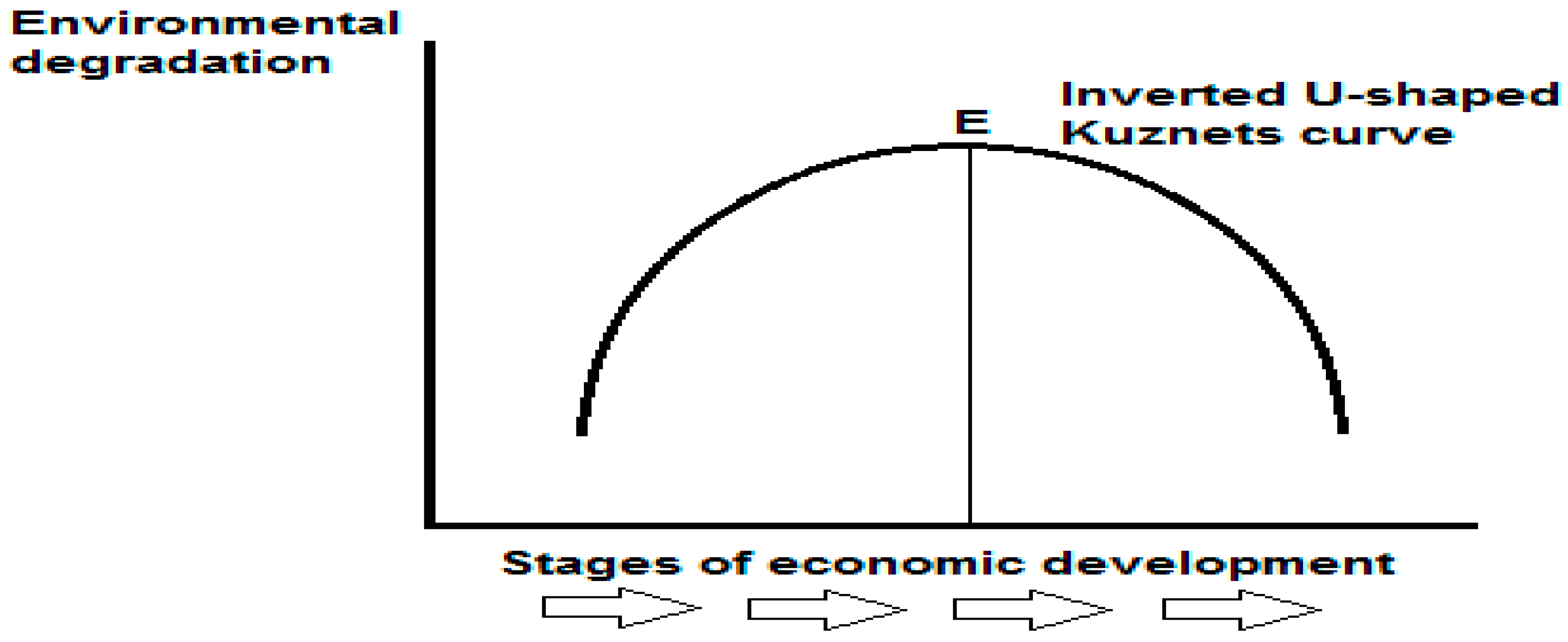
The form EKC takes in an economy over time is shown in Figure 1. As a country starts making its way up the economic ladder, the immediate effect of that growth is an increase in environmental degradation. It is the part of the Kuznets curve before point E, which is a turning point. There is a reliable and widely applicable logic behind a growing economy experiencing an increase in environmental degradation. Since the economy is expanding and income in the country is increasing, it is pretty evident that the production level will rise. These production initiatives most likely involve activities leading to higher emissions into the environment, hence causing environmental degradation. Point E in Figure 1 is the turning point where environmental degradation starts making a U-turn and reduces as the country keeps growing in economic terms. After the turning point E, while income is still increasing, environment degradation starts to decline, and the EKC ends up being an inverted U-shape. In a sample of countries from mixed regions, Apergis et al. [28] have conducted a panel analysis and have manifested a causality among emissions, energy usage, and income. Another study that divided the sample into high-, middle-, and low-income countries has been conducted by Ulucak and Bilgili [29], and the existence of an EKC has been supported in the selected sample countries, and an inverted U-shaped relation is found between income and emissions.
In the context of EKC, the idea of the pollution haven hypothesis (PHH) is also worth mentioning. According to the hypothesis, in countries where environmental regulations are strict, it is costlier for large industries to operate and perform environmentally deteriorating operations. Conversely, in developing countries, where environmental regulations are not as strict, it is cheaper to set up a pollutant factory while the labor is also cheap. It leads factories and industries to outsource work and move to these developing nations since they are cheaper with lower environmental standards [9]. Zheng and Shi [30] study the existence of the hypothesis in the context of China and argue that better environmental policies in the country are a driver of the relocation of industrial activities.
Many macro and microeconomic factors are associated with emissions in a country. Some of the factors that are analyzed in this piece of research are income, square of income, FDI, FMD, trade openness, and energy intensity. The way increasing income affect environmental degradation is already mentioned through the Kuznets curve. When it comes to the effects of FMD on emissions, Abbasi and Riaz [31] utilize a vector auto-regressive (VAR) approach to study this correlation and have mentioned that financial development and trade liberalization do not help to mitigate the effects of environmental degradation and are responsible for an increase in this ecological destruction. On the other hand, Shahbaz et al. [32] showed in their study that FMD tends to raise the environmental quality in Malaysia. In later stages of development when the country has gained enough economic development, financial development might help with reducing emissions, but those effects are still minimal. Several financial factors, including FDI, private sector credit, and stock market turnover, are shown to increase CO2 emissions. With ease in the stock market liquidity constraints, firms can expand their production and use more energy, which consequently leads to emissions.
Xiaong et al. [20] investigated the regional differences in the effects of FMD on emissions on a panel dataset from China. It is mentioned that parts of China that are already well developed could reduce emissions with more financial development while for other less developed regions in the country, financial development tends to increased emissions, leading to environmental degradation. Market forces and institutional constraints are said to be preventing financial development from bringing improvements in the environments. Therefore, it has been suggested not to rely on financial development only since there are conflicting results and economies should implement policies like financing greener activities on a local level in order to ensure that the environment gets improved.
The idea of developed economies being in a better position to tackle the complications of the environment and environmental quality through financial development makes theoretical and practical sense in several ways. For instance, developed countries have already achieved an advanced level of technological evolution and can optimize their business activities. For developing regions, the stage of achieving an utmost efficiency regarding production is yet to be achieved, which can worsen the environment with more production. On the other hand, developed countries can grow without worsening the environment because of their advanced knowledge and processes. It is a point to ponder for developing countries to explore more options that can help them to achieve a higher production while keeping emissions and other environmentally destructive process afar. Adams and Klobodu [33] suggested that the political regime in a country can play a role in connecting financial development to CO2 emissions, while urbanization can worsen the environment.
FDI can have a strong influence on pollution and Thorbecke and Salike [34] mentioned in their study that due to the regional production networks, the FDI profile of East Asia is becoming very specific and improving trade relations in the region. Also, countries are trading for parts and components of products more than final manufactured goods. An example of this is electronics that can travel in parts without any hassle. In this networked trade, the infrastructure of the host countries plays a vital role in determining if it can handle higher levels of trade. For instance, higher trade of electronics from East Asia has improved the trade profile of host countries working with Japan. In such fragmented trade activities, the total cost of the trade is a sum of service link cost and the marginal cost of production while the quality of the physical market and institutional infrastructure matter as well.
Additionally, parts of Asia, such as inland China and India, are making labor much cheaper, which attracts higher FDI from the developed world. Dinda [35] argued that higher FDI has a strong role in the determination of the EKC hypothesis. When higher trade increases the size of an economy and its industry, pollution becomes inevitable. However, the fact that trade can also improve the environment of the host country since composition and technique effects cannot be denied. When industries swap activities through trade, they also exchange the level of pollution that they create and while pollution increases in one part of the world, it reduces in the other, leading to composition effects. Technique effect is when countries with higher industrial growth and more environmental regulations come up with better and fewer-pollutant technologies to continue their production activities.
Trade openness in a country influences the emission rate, and Mutascu [36] talked about the existence of a business cycle between the two variables. There does not seem to be a strong connection between CO2 emissions and trade openness in a short-term. Conversely, Shahbaz et al. [37] argued that trade openness leads to destruction in the environment in low-, middle-, and high-income countries. There is no denial of the fact that trade openness helps countries gain economic, political, financial, and strategic gains and assists nations to upgrade their presence in the world. However, when the trade becomes more open in a country, trade volume increases and there is a higher inflow and outflow of products. As a result, more industrial units are developed in the country that consumes energy, which is likely to lead to CO2 emissions and environmental degradation. Kim et al. [38] also argued that trade improves the economy while deteriorating the environment.
Some studies have been conducted in the Asian region. For example, Zhu et al. [15] analyzed the effects of FDI, income, and energy usage on CO2 emission and land on the inference that all variables strongly influence emissions in the Association of Southeast Asian Nations (ASEAN) region. It has been mentioned that with a higher level of FDI, effects of high emissions seem to get mitigated in ASEAN countries while economic growth has shown to increase emissions. Atici [16] conducted a similar analysis and concluded that with higher trade figures, emissions tend to increase in ASEAN countries, independent of whether the country is in a developed, developing, or late-developing state. Ahmed et al. [17] mentioned that CO2 emissions in South Asia are influenced by a variety of factors including trade openness, income, population, and energy consumption. They use panel data of five South Asian economies from 1971–2013 and prove a long-run cointegration between pollution and other mentioned factors. With proof of a bi-directional relationship among emissions and other macroeconomic factors, the study provided robust empirical evidence while leaving space for the analysis to be conducted for other Asian regions. Al-Mulali et al. [19] indicated the existence of EKC in a panel of seven regions including East Asia and Pacific from 1980–2010. With renewable energy shown to be improving the environment, both income and population are seen to complement the existence of EKC in the selected sample. Further, they could not establish a relationship between trade openness and emissions in the East Asia and Pacific region. Nevertheless, the existence of spatial dependency has not been incorporated in the study which provides a lead to conduct more spatial studies on EKC and its prevalence in East Asia.
Behera and Dash [18] conducted a panel data study on South and Southeast Asian region to find out the existence of the causality of urbanization, energy usage and FDI on emissions. With the help of an analysis conducted on a set of 17 countries using the data from 1980–2012, the causality relationships have been proven. Specifically, for middle-income countries, primary and secondary fossil fuels are said to have a substantial impact on emissions, leading to a higher level of greenhouse gases. While the study itself has not incorporated the spatial dimension in the model, it has been mentioned that spatial concentration has gained popularity in the available literature. There is a need to incorporate spatial dimension in studies like this because emissions are not a stand-alone problem of a specific region and do influence the surrounding demographics to a significant extent.
While a good number of research pieces that have been established on the topic of EKC and its implication across the world, there is still a lack of evidence as to how EKC applies in the East Asian region with the presence of spatial dependency. However, some studies do address the idea of spatial dependency in the environmental profile of China. For instance, Hao et al. [21] analyzed EKC in China on a provincial level and investigated the spatial effects. It was concluded in the study that since 2006, spatial effects have started to emerge in China and their effects have become meaningful. To keep the study less biased, data for multiple pollutants has been collected from 30 provinces, which have proved the existence of EKC. Another inference from the analysis is that good governance helps to reduce the adverse effects of environmental degradation.
While conducting an analysis of spatial dependency on the environmental profile of China, Jiang et al. [22] argued that the inverted U-shaped relationship does exist between income and energy intensity. Additionally, the energy intensity of one province of China has an impact on other provinces while FDI is showed spillover effects across provinces by reducing energy intensity. It is concluded that when the labor/capital ratio in one province changes, it has potential effects on the energy intensity of neighboring provinces too. Using the STIRPAT model, Liu et al. [39] applied spatial econometric on the determinants of CO2 emissions of Chinese regional data. They report that the indirect effect of income per capita, energy intensity, and openness are negative on the CO2 emissions. However, direct effects of such variables are found responsible for increasing CO2 emissions. Xiong et al. [23] found the spatial correlation with different types of industrial pollution. The inverted U-shape relationship is reported between urban agglomeration and pollution along with strong spatial effects.
Further, the effects of population and industry are found responsible for environmental degradation. Zhao et al. [6] concluded a similar spatial pattern in terms of sulfur dioxide in China from 2001–2014. Hao et al. [24] concluded the existence of spatial effects as well in China. It is argued that coal consumption in China does potentially lead to higher emissions and environmental degradation while the EKC seems to exist in China. Additionally, due to the existence of spatial effects, coal consumption in one province of the country can lead to a higher level of emissions in the other.
Liu et al. [25] conducted a spatial analysis on China and mentioned that there is an existence of spatial correlation in 30 selected provinces of China and as time passes, this spatial binding keeps getting more intense. Two main analyzed instruments during the research are urbanization and eco-environment. It is argued that as the distance between selected provinces starts increasing, spatial dependency keeps getting smaller. The conclusion leads to a strong implication that provinces closer to each other can influence each other’s environment and urbanization, while with distance, the effects seem to fade away. It also provides applicable policy guidance for Chinese provinces to apply functional governance since their urbanization does not only decide their economic fate, it also puts an impact on the neighboring provinces of the country. Another study conducted on provincial panel data of China about the spatial presence in the environmental setting is by Wang et al. [26] who utilized a period 1995–2011, and by using the STIRPAT model, regional imbalances between CO2 emissions have been observed in Chinese provinces. The existence of EKC is proven in China with strong policy implications for rigorous regulations to reduce the effects of environmental degradation.
Additionally, the development of advanced technology, promoting renewable and recycled energy and the development of the tertiary industry have been suggested to be some significant factors useful in mitigating the adverse effects of pollution. Using panel data from 338 cities in China, Zhan et al. [27] analyzed spatial differences between the cities and mention that both socioeconomic and natural factors play a role in the intensity of these spatial effects in China. Other than China, some studies are conducted considering the spatial dependency. For example, Wang et al. [40] studied the existence of EKC on a global level with a spatial dependency. They could not complement the existence of EKC, but they prove the relationships between energy consumption, income, and emissions. It is also argued that the investigated factors of the neighboring countries are potentially affecting the emissions rate of the local country, proving the existence of spatial effects. Using city-level data for a period 2003–2013, Yi et al. [41] investigated the spatial effects of different factors. They report that urbanization increases CO2 emissions, but its spatial effects help in reducing it. Further, the role of green FDI has been found helpful in reducing pollution.
A wide variety of studies conducted on the topic so far is mostly limited to testing the existence of EKC in the Asia region [3,19] or to limit the scope to find the monotonic effect of different variables on the pollution emissions in South and Southeast Asia [15,16,17,18] and does not proceed to incorporate spatial effects. Other than studies conducted on China [1,2,5,6,7,8,21,22,23,24,25,26,27], no extensive research has been done on EKC with the prevalence of spatial effects in the panel of East Asia region which is a vast research gap that this study focuses on filling.
3. Methods
To test the EKC hypothesis and to investigate the effects of income, FMD, trade openness, FDI, and energy intensity, we hypothesize the following model:
where, ln is the natural log, COPCit is the CO2 emissions per capita, GDPCit is the real gross domestic product (GDP) per capita, FMit is the FMD proxy by domestic credit to the private sector ratio to GDP, FDIit is the net FDI inflows ratio to GDP, TOit is the trade openness and is a ratio of sum of exports and import and GDP, EIit is the energy intensity as ratio of energy supply to GDP, t is the period of 1991–2014, and i is for each of the six East Asian countries, i.e., China, Japan, Hong Kong, Macao, Mongolia, and the Korea Republic. Fixed Effects (FE) are introduced in Equation (1) via intercept , which is initially assumed to be varying over countries i and time t. Later, , , and may be replaced with in Equation (1) for only the countries’ varying effects (FE- Country), for only time-variant effects (FE-Time), and for pooled ordinary least square (OLS), respectively. All data is sourced from World Development Indicators (WDI) [42] and is available as supplementary material. Taiwan and North Korea are ignored due to the non-availability of data. An FDI series of Hong Kong is interpolated for some missing years’ data using linear interpolation method. A period is limited to the year 2014 due to non-availability of energy and pollution data from WDI after 2014 to maintain a homogenous source of data. GDP per capita and its square are incorporated in Equation (1) to test the EKC hypothesis.
Equation (1) may be regressed using pooled OLS and fixed effects (FE) at first, and then a Lagrange multiplier (LM) and LM robust tests may be applied afterwards to access the presence of spatial dependence in the model [43]. In the presence of significant spatial dependency, the spatial Durbin model (SDM) may be applied [44] on Equation (1) in the following way:
Here, W is the weight matrix that is 6 × 6 in dimension and showing the elements (wij), which are having distances between i and j countries. W is normalized via the maximum distance from each row of the matrix [45]. Based on the definition of W, shows the spatial dependence of CO2 emissions per capita among countries. Further, the captures the spatial effects of neighboring countries’ independent variables on the local CO2 emissions per capita and captures the direct effects of local country’s independent variables on the local CO2 emissions per capita. After estimating the SDM of Equation (2), the likelihood ratio (LR) and Wald tests may be applied to test the null hypotheses H01: and H02: to verify the suitability and superiority of SDM over the spatial auto-regressive (SAR) method and spatial error model (SEM). The rejection of both hypotheses simultaneously corroborates that SDM cannot be simplified for SAR and SEM and SDM is the most efficient choice in this case [44].
4. Data Analyses and Discussions
Figure 2 and Figure 3 below show the trends of GDP per capita and CO2 emissions per capita respectively in our selected sample of six countries in the East Asian region. Average GDP per capita of Japan was at the highest level among others and this position was the same for CO2 emissions. In the first half of the selected period, CO2 emissions and GDP per capita moved in the same positive direction mostly, but in the second half of the period, both started moving in the opposite direction as well in the cases of Japan, Macao, Korea, and Hong Kong, and higher GDP per capita resulted in a decline in CO2 emissions in some cases. This result shows on the inverted U-shaped EKC with CO2 emissions increasing with GDP per capita and then declining afterwards. On the other hand, a positive relationship between said variables was observed throughout the period for the comparatively low-income countries China and Mongolia. Further, CO2 emissions per capita were growing at faster rate, mostly in these two economies during 2009–2014.
After some graphical observations, we tested the existence of a long-run relationship in the modelled variables through panel cointegration tests. In the Table 1, a Pedroni [46] test shows that four out of seven statistics proved the existence of cointegration in our model. A Kao [47] test also corroborated the existence of cointegration at a 1% level of significance. Further, a Johansen–Fisher test proposed by Maddala and Wu [48] gave evidence of six significant cointegration vectors. The results of three cointegration tests provided sufficient information for the existence of a long run relationship in our proposed model. Therefore, we proceeded for long-run estimates.
After a cointegration analysis, Table 2 shows the estimated non-spatial model through a pooled OLS, dynamic OLS, and fixed effects. The existence of FE needed to be verified using the LR test. The estimated chi-square values (p-values) from the LR test were found to be 121.94 (0.000), 59.19 (0.000), and 182.63 (0.000) for FE-country, FE-time, and FE-both, respectively. Therefore, all types of regressed FE models were suitable for our estimations. Considering one lag and one lead of each variable, dynamic OLS was also employed to verify the direction of relationships. The positive (negative) coefficients of lnGDPCit (lnGDPCit2) corroborated the inverted U-shape relation or the EKC hypothesis in all estimated models. The effect of FMit was found to be negative and significant in the pooled OLS and FE-time estimates, and insignificant in the rest of the estimates. The effect of FDIit was positive and significant in all estimated models except for the results of the dynamic OLS. Trade openness showed positive and significant influence on the CO2 emissions per capita in all models except FE-both. Lastly, the effect of energy intensity was found to be positive and significant in all the estimated models.
Moreover, the suitability of spatial lag and/or error models was tested using LM and LM robust tests. Both tests verified the suitability of both spatial lag and error models in the estimated pooled OLS and FE-both. In the case of FE-country and FE-time estimates, the LM test verified both spatial error and lag models, but the LM robust test only favored the spatial lag model and did not favor the spatial error model. In the case of FE-time estimates, the LM robust test did not favor the spatial lag model but favored the spatial error model. However, LM and LM robust tests provided sufficient evidence for the existence of spatial dependency in the hypothesized models and ignoring spatial dependency may be counted for a specification bias.
After confirming the spatial dependency in the model, we regressed the SDM with the FE and random effect (RE) and have reported the results in Table 3. Before discussing the detailed results, we note that we applied a Wald test to confirm that either SDM may be reduced to SAR or SEM. In both estimations of SDM-FE and SDM-RE, H01 and H02 mentioned in the methodology section were rejected at the 1% level of significance, which means that SDM was more efficient in both estimations of FE and RE. Further, LR test was applied to compare the SDM with SAR and SEM, and this test favored SDM again. Moreover, the Hausman test was applied on a null hypothesis of “SDM-RE is suitable.” The null hypothesis could not be rejected, therefore we considered the SDM-RE as the most suitable choice.
In the SDM-RE estimations, all coefficients of weighted variables were statistically significant except GDP per capita and energy efficiency. Therefore, spillover effects are presented from the rest of the variables including CO2 emissions per capita. Liu et al. [25] agreed with the idea of spatial dependency as well, and in their study on China, they have argued that Chinese provinces are spatially dependent on each other in terms of eco-environment while urbanization has a strong role in that as well. Ge et al. [7] agreed to the concept of spatial dependency in terms of emissions in China. Chen et al. [2] argued about a strong existence of spatial dependency in the region mentioning that other than environmental degradation, pollution has spatial effects on public health as well.
In the association of GDP per capita and CO2 emissions per capita, the inverted U-shape relationship was found in the point, direct, and total estimates. The existence of the EKC hypothesis was corroborated in East Asia with this inverted U-shape relationship. Further, the U-shape relationship was estimated in the indirect estimates, which may be ignored due to the insignificant coefficient of W*lnGDPCit. However, the estimated negative indirect effect of GDP per capita is in line with the results of a spatial study on China by Liu et al. [39]. FMD had an insignificant effect on the CO2 emissions per capita in the point and direct estimates. This means that the local FMD had neither negative nor positive environmental effects. However, the coefficient in the indirect and total estimates was positive and significant. Therefore, we may conclude that the spillover effect of neighboring countries’ FMD and total effect of FMD had a positive contribution in the accumulation of local CO2 emissions per capita. FDI had a positive and significant effect on the CO2 emissions per capita in the point and direct estimates. This result indicates that with a higher net inflow of FDI in the East Asian region, the environment becomes deteriorated.
Additionally, with the higher environmental degradation in the region with higher FDI, it was illustrated that a large number of FDI was being attracted to the pollution-oriented industrial sector in East Asia. This result is in contrast of the finding of Zhu et al. [15] who found a positive environmental effect of FDI in five ASEAN countries, and Atici et al. [16] found an insignificant effect of FDI on pollution in ASEAN countries. In the indirect effects, the coefficient of FDI was negative and significant. This shows that the net FDI inflows in the neighboring countries have a pleasant environmental effect on the local CO2 emissions per capita. This is corroborated with the study of Yi et al. [41] for China and with the Jiang et al. [22] who find a positive spillover effects of FDI through reducing energy intensity in China. This result also corroborates the fact that East Asian countries are competitors in attracting the net FDI inflows and increasing FDI in neighboring countries are reducing the chance of FDI inflows in the local country and thus may help in reducing local CO2 emissions per capita. The production setup and activities of East Asian investors are spread across various countries as well [34]. Therefore, FDI in the dirty production process of one country may reduce the chance of installing this production process in another country. Therefore, the spillover effects of neighboring countries’ FDI may have pleasant local environmental effects. This leads to the idea of a displacement hypothesis as well that argues that although developed countries move to the developing ones for more polluting industry activities, it makes the developing countries the producers of dirty products and eventual exporters. On the other hand, developed countries are the ones that are importing these dirty products, and their consumption remains higher than that of the developing ones.
Trade openness was seen to have a positive and significant impact on CO2 emission per capita, and this is true for all the estimated coefficients. Negative environmental effects of trade are in line with the findings of Atici et al. [16] for ASEAN and Japan and Liu et al. [39] for China, but are in contrast with the insignificant relation reported by Al-Mulali [19] for East Asia and the Pacific. East Asian countries are famous for exporting the industrial products, and increasing trade openness is responsible for the production of more industrial products using energy and emitting CO2 emissions. Further, adverse environmental effects of FDI and trade openness corroborated the PHH in East Asia. Moreover, the coefficient of the indirect effect was larger than the direct effect. Therefore, we may conclude that increasing trade openness in neighboring countries had an adverse environmental effect, even larger than that of local trade openness. Conversely, Atici [16] provides a different approach to the idea of trade openness and spatial effects, and using the example of Japan, it is mentioned that trade does not increase emissions due to the environmental awareness of Japan.
Lastly, energy intensity had a positive and significant effect on CO2 emissions per capita in the point, direct, and total estimates. Therefore, the increasing energy requirement for each unit of production was responsible for more pollution. This result also reflected that most of the energy consumption had its pollution origins in East Asia. The indirect effect of energy intensity showed a negative and significant effect on CO2 emissions per capita. First of all, we may ignore this result due to the insignificant coefficient of W*lnEIit. Second, if we consider its significant indirect effect, then it shows that increasing energy intensity in a neighboring country helps in reducing local CO2 emissions per capita. Then, this result may be reflected by negative indirect effect of FDI as most of the FDI in energy intensive projects may shift in neighboring countries. As a result, increasing the energy intensity of neighboring countries may have local positive environmental spillover effects.
5. Conclusions and Implications
We investigate the EKC hypothesis in the East Asian countries using the period 1991–2014 along with the impact of FDI, FMD, trade openness, and energy intensity on the CO2 emissions per capita. For this purpose, we regressed the non-spatial models and tested the existence of spatial dependency in the model. Through LM and LM robust tests, we found the existence of spatial dependency in our hypothesized model. Further, we regressed the SDM and have confirmed its suitability over SAR and SEM. Moreover, a Hausman test was applied to test the efficiency of SDM-FE and SDM-RE, and we found that SDM-RE was suitable. In the SDM-RE estimates, we found the inverted U-shaped association between income and CO2 emissions. Hence, the EKC hypothesis was proven true in the East Asian countries. However, spillover effects of GDP per capita were found insignificant through the insignificant coefficient of the weighted GDP per capita variable.
The effect of local FMD on local CO2 emissions per capita was found to be insignificant, but spillover effects of neighboring countries’ FMD showed a positive effect on the local CO2 emissions per capita. The significant spillover effects of FMD also highlighted the importance of spatial analysis as an effect of FMD was found to be insignificant in unlike most of estimated non-spatial models that estimated an insignificant direct effect. Local FDI inflows were found to be responsible for environmental degradation. This result indicated that most of FDI was in pollution-oriented industries, which proved the existence of the PHH in the East Asia region. On the other hand, spillover effects of neighboring countries’ FDI inflows had positive local environmental effects via reducing local CO2 emissions per capita. This result corroborated a fact that the production processes were spread over the different locations and countries, and the installation of a dirty production process in one country may reduce the chance to be installed the same in another country and may consequently reduce the chance of pollution there.
Both local and neighboring countries’ trade openness had negative local environmental effects through increasing local CO2 emissions per capita. This led to an inference that emissions in a country of the East Asian region did not only influence the environmental profile of that specific country, but these effects were transferred to the neighboring nations as well, which could eventually affect the entire region in a negative way. Further, the magnitude of the spillover effect was larger than that of the local effect. The East Asia region is famous for exporting industrial products, and the industrial sector consumes more energy and may produce more pollution compared to agriculture and the service sectors. Therefore, increasing trade openness may expand the share of the industrial sector in East Asia and is responsible for environmental degradation. Last, local increasing energy intensity was responsible for increasing local CO2 emissions per capita, and spillover effects of energy intensity were found to be insignificant through the weighted energy intensity variable. The negative environmental effects of energy intensity are line with the fact that more than 80% of energy consumption is from fossil fuel in East Asia.
Based on the investigated results, we suggest that East Asian countries should consider the environmental effects before any target of economic growth. It is crucial to keep the environmental effects of growth in context because the consequences can have wider influences on the region and neighboring countries. It can be seen that local FDI and trade openness had an adverse effect on the environment. The results of the study have strong implications for the East Asian region and provide a guideline for policy formation in the region. It is time for economies to give critical thought to the decision of attracting more foreign investment into the country as it will consequently impact the environment in a negative way. At this point, the concept of opportunity cost can also be incorporated by these economies to consider whether getting all the FDI and economic benefit is offsetting enough for the resultant emissions.
On top of that, the same approach should be given to liberalization and trade openness as well since the environmental effects are altogether negative. There is a crucial need for the economies to reconsider their environmental policies pollution haven in the East Asian region regarding trade agreements since the eventual long-term effects might not be what they think they would be. Countries need to compare the benefit of FDI and trade openness and the cost of environmental degradation and come up with a balance that can provide them with more net social benefits. Energy efficiency policies can also assist in creating that balance and making industrial production less harmful to the environment. While formulating energy and environmental policies, spillover effects of FMD, FDI, and trade openness should be given significant weight, along with local effects, since they can take the discussion in a different direction. Moreover, estimated coefficients of direct and indirect effects may be considered for any environmental protection policy, and estimated spatial effects should be considered while forming the local policies.
Supplementary Materials
The following are available online at https://www.mdpi.com/2071-1050/11/1/13/s1: Data.xlsx.
Author Contributions
Conceptualization, H.M. and O.A.B.; methodology, H.M.; software, H.M.; validation, H.M. and M.F.; formal analysis, H.M.; investigation, O.A.B. and M.F.; data collection, O.A.B.; writing—original draft preparation, O.A.B. and M.F.; writing—review and editing, H.M. and M.F.; supervision, H.M.; project administration, H.M.
Funding
This research received no external funding.
Conflicts of Interest
The authors declare no conflict of interest.
References
- Auffhammer, M.; Carson, R. Forecasting the Path of China’s CO2 Emissions Using Province-Level Information. J. Environ. Econ. Manag. 2008, 55, 229–247. [Google Scholar] [CrossRef]
- Chen, X.; Shao, S.; Tian, Z.; Xie, Z.; Yin, P. Impacts of Air Pollution and its Spatial Spillover Effect on Public Health Based on China’s Big Data Sample. J. Clean. Prod. 2017, 142, 915–925. [Google Scholar] [CrossRef]
- Le, T.; Quah, E. Income Level and the Emissions, Energy, and Growth Nexus: Evidence from Asia and the Pacific. Int. Econ. 2018, 156, 193–205. [Google Scholar] [CrossRef]
- Nepal, R.; Jamasb, T.; Tisdell, C.A. On the environmental impacts of market-based reforms: Evidence from the European and Central Asian transition economies. Renew. Sustain. Energy Rev. 2017, 73, 44–52. [Google Scholar] [CrossRef]
- Guo, J.; Xu, Y.; Pu, Z. Urbanization and Its Effects on Industrial Pollutant Emissions: An Empirical Study of a Chinese Case with the Spatial Panel Model. Sustainability 2016, 8, 812. [Google Scholar] [CrossRef]
- Zhao, X.; Deng, C.; Huang, X.; Kwan, M.-P. Driving Forces and the Spatial Patterns of Industrial Sulfur Dioxide Discharge in China. Sci. Total Environ. 2017, 577, 279–288. [Google Scholar] [CrossRef] [PubMed]
- Ge, X.; Zhou, Z.; Zhou, Y.; Ye, X.; Liu, S. A Spatial Panel Data Analysis of Economic Growth, Urbanization and NOx Emissions in China. Int. J. Environ. Res. Public Health 2018, 15, 725. [Google Scholar] [CrossRef]
- Pu, Z. Time-Spatial Convergence of Air Pollution and Regional Economic Growth in China. Sustainability 2017, 9, 1284. [Google Scholar] [CrossRef]
- Yang, N.; Zhang, Z.; Xue, B.; Ma, J.; Chen, X.; Lu, C. Economic Growth and Pollution Emission in China: Structural Path Analysis. Sustainability 2018, 10, 2569. [Google Scholar] [CrossRef]
- Baker, L. Of Embodied Emissions and Inequality: Rethinking Energy Consumption. Energy Res. Soc. Sci. 2018, 36, 52–60. [Google Scholar] [CrossRef]
- Pata, U.K. Renewable energy consumption, urbanization, financial development, income and CO2 emissions in Turkey: Testing the EKC hypothesis with structural breaks. J. Clean. Prod. 2018, 187, 770–779. [Google Scholar] [CrossRef]
- Huang, L.; Zhao, X. Impact of financial development on trade-embodied carbon dioxide emissions: Evidence from 30 provinces in China. J. Clean. Prod. 2018, 198, 721–739. [Google Scholar] [CrossRef]
- La Rovere, E.L.; Grottera, G.; Wills, W. Overcoming the financial barrier to a low emission development strategy in Brazil. Int. Econ. 2018, 155, 61–68. [Google Scholar] [CrossRef]
- Gallagher, K.P.; Kamal, R.; Jin, J.; Chen, Y.; Ma, X. Energizing development finance? The benefits and risks of China’s development finance in the global energy sector. Energy Policy 2018, 122, 313–321. [Google Scholar] [CrossRef]
- Zhu, H.; Duan, L.; Quo, Y.; Yu, K. The Effects of FDI, Economic Growth and Energy Consumption on Carbon Emissions in ASEAN-5: Evidence from Panel Quantile Regression. Econ. Model. 2016, 58, 237–248. [Google Scholar] [CrossRef]
- Atici, C. Carbon Emissions, Trade Liberalization, and the Japan–ASEAN Interaction: A Group-Wise Examination. J. Jpn. Int. Econ. 2012, 26, 167–178. [Google Scholar] [CrossRef]
- Ahmed, K.; Rehman, M.; Ozturk, I. What Drives Carbon Dioxide Emissions in the long-run? Evidence from Selected South Asian Countries. Renew. Sustain. Energy Rev. 2017, 70, 1142–1153. [Google Scholar] [CrossRef]
- Behera, S.; Dash, D. The Effect of Urbanization, Energy Consumption, and Foreign Direct Investment on the Carbon Dioxide Emission in the SSEA (South and Southeast Asian) Region. Renew. Sustain. Energy Rev. 2017, 70, 96–106. [Google Scholar] [CrossRef]
- Al-Mulali, U.; Ozturk, I.; Solarin, S. Investigating the Environmental Kuznets Curve Hypothesis in Seven Regions: The Role of Renewable Energy. Ecol. Indic. 2016, 67, 267–282. [Google Scholar] [CrossRef]
- Xiaong, L.; Tu, Z.; Ju, L. Reconciling Regional Differences in Financial Development and Carbon Emissions: A Dynamic Panel Data Approach. Energy Procedia 2017, 105, 2989–2995. [Google Scholar] [CrossRef]
- Hao, Y.; Wu, Y.; Wang, L.; Huang, J. Re-Examine Environmental Kuznets Curve in China: Spatial Estimations using Environmental Quality Index. Sustain. Cities Soc. 2018, 42, 498–511. [Google Scholar] [CrossRef]
- Jiang, L.; Folmer, H.; Ji, M. The Drivers of Energy Intensity in China: A Spatial Panel Data Approach. China Econ. Rev. 2014, 31, 351–360. [Google Scholar] [CrossRef]
- Xiong, L.; de Jong, M.; Wang, F.; Cheng, B.; Yu, C. Spatial spillover effects of environmental pollution in China’s central plains urban agglomeration. Sustainability 2018, 10, 994. [Google Scholar] [CrossRef]
- Hao, Y.; Kiu, Y.; Weng, J.; Gao, Y. Does the Environmental Kuznets Curve for Coal Consumption in China Exist? New Evidence from Spatial Econometric Analysis. Energy 2016, 114, 1214–1223. [Google Scholar] [CrossRef]
- Liu, N.; Liu, C.; Xia, Y.; Da, B. Examining the Coordination between Urbanization and Eco-Environment using Coupling and Spatial Analyses: A Case Study in China. Ecol. Indic. 2018, 93, 1163–1175. [Google Scholar] [CrossRef]
- Wang, S.; Fang, C.; Wang, Y. Spatiotemporal Variations of Energy-Related CO2 Emissions in China and its Influencing Factors: An Empirical Analysis Based on Provincial Panel Data. Renew. Sustain. Energy Rev. 2016, 55, 505–515. [Google Scholar] [CrossRef]
- Zhan, D.; Kwan, M.-P.; Zhang, W.; Yu, X.; Meng, B.; Liu, Q. The Driving Factors of the Air Quality Index in China. J. Clean. Prod. 2018, 197, 1342–1351. [Google Scholar] [CrossRef]
- Apergis, N.; Payne, J.; Menyah, K.; Rufael, Y. On the Causal Dynamics between Emissions, Nuclear Energy, Renewable Energy, and Economic Growth. Ecol. Econ. 2010, 69, 2255–2260. [Google Scholar] [CrossRef]
- Ulucak, R.; Bilgili, F. A Reinvestigation of EKC Model by Ecological Footprint Measurement for High, Middle and Low-Income Countries. J. Clean. Prod. 2018, 188, 144–157. [Google Scholar] [CrossRef]
- Zheng, D.; Shi, M. Multiple environmental policies and pollution haven hypothesis: Evidence from China’s pollution industries. J. Clean. Prod. 2017, 141, 295–304. [Google Scholar] [CrossRef]
- Abbasi, F.; Riaz, K. CO2 Emissions and Financial Development in an Emerging Economy: An Augmented VAR Approach. Energy Policy 2016, 90, 102–114. [Google Scholar] [CrossRef]
- Shahbaz, M.; Solarin, S.; Mahmood, H.; Mohamed, A. Does Financial Development Reduce CO2 Emissions in the Malaysian Economy? A Time Series Analysis. Econ. Model. 2013, 35, 145–152. [Google Scholar] [CrossRef]
- Adams, S.; Klobodu, E. Financial Development and Environmental Degradation: Does Political Regime Matter? J. Clean. Prod. 2018, 197, 1472–1479. [Google Scholar] [CrossRef]
- Thorbecke, W.; Salike, N. Understanding FDI and production networks in East Asia. Asian-Pac. Econ. Lit. 2016, 30, 57–71. [Google Scholar] [CrossRef]
- Dinda, S. Environmental Kuznets Curve Hypothesis: A Survey. Ecol. Econ. 2004, 49, 431–455. [Google Scholar] [CrossRef] [Green Version]
- Mutascu, M. A Time-Frequency Analysis of Trade Openness and CO2 Emissions in France. Energy Policy 2018, 115, 443–455. [Google Scholar] [CrossRef]
- Shahbaz, M.; Nasreen, S.; Ahmed, K.; Hammoudeh, S. Trade Openness–Carbon Emissions Nexus: The Importance of Turning Points of Trade Openness for Country Panels. Energy Econ. 2017, 61, 221–232. [Google Scholar] [CrossRef]
- Kim, D.; Suen, Y.; Lin, S. Carbon Dioxide Emissions and Trade: Evidence from Disaggregate Trade Data. Energy Econ. 2018, 78, 13–28. [Google Scholar] [CrossRef]
- Liu, Y.; Xiao, H.; Zikhali, P.; Lv, Y. Carbon emissions in China: A spatial econometric analysis at the regional level. Sustainability 2014, 6, 6005–6023. [Google Scholar] [CrossRef]
- Wang, Y.; Kang, L.; Wu, X.; Xiao, Y. Estimating the Environmental Kuznets Curve for Ecological Footprint at the Global Level: A Spatial Econometric Approach. Ecol. Indic. 2013, 34, 15–21. [Google Scholar] [CrossRef]
- Yi, Y.; Ma, S.; Guan, W.; Li, K. An empirical study on the relationship between urban spatial form and CO2 in Chinese cities. Sustainability 2017, 9, 672. [Google Scholar] [CrossRef]
- World Development Indicators; The World Bank: Washington, DC, USA, 2018.
- Elhorst, J. Matlab software for spatial panels. Int. Reg. Sci. Rev. 2012, 35, 1–17. [Google Scholar] [CrossRef]
- Lesage, J.P.; Pace, R.K. Introduction to Spatial Econometrics, 1st ed.; CRC Press: New York, NJ, USA, 2009; ISBN 10:142006424X. [Google Scholar]
- Elhorst, J. Dynamic models in space and time. Geogr. Anal. 2001, 33, 119–140. [Google Scholar] [CrossRef]
- Pedroni, P. Panel cointegration: Asymptotic and finite sample properties of pooled time series tests with an application to the PPP hypothesis. Econom. Theory 2004, 20, 579–625. [Google Scholar] [CrossRef]
- Kao, C. Spurious regression and residual-based tests for cointegration in panel data. J. Econom. 1999, 90, 1–44. [Google Scholar] [CrossRef]
- Maddala, G.S.; Wu, S. A comparative study of unit root tests with panel data and a new simple test. Oxf. Bull. Econ. Stat. 1999, 61, 631–652. [Google Scholar] [CrossRef]
Figure 1.
The EKC.

Figure 2.
GDP per capita.

Figure 3.
CO2 emissions per capita.


Table 1.
Panel cointegration tests.
| Statistic | Probability | |
|---|---|---|
| Pedroni Residual Cointegration Test | ||
| Panel v-Statistic | −1.451 | 0.927 |
| Panel rho-Statistic | 1.761 | 0.961 |
| Panel PP-Statistic | −2.650 | 0.004 |
| Panel ADF-Statistic | −1.935 | 0.027 |
| Group rho-Statistic | 2.462 | 0.993 |
| Group PP-Statistic | −4.162 | 0.000 |
| Group ADF-Statistic | −1.336 | 0.091 |
| Kao Residual Cointegration Test | ||
| Augmented Dickey Fuller | −2.809 | 0.003 |
| Johansen Fisher Panel Cointegration Test | ||
| Cointegration Equations: Fisher Statistic from the Trace Test | ||
| None | 285.300 | 0.000 |
| At most 1 | 332.300 | 0.000 |
| At most 2 | 235.500 | 0.000 |
| At most 3 | 147.200 | 0.000 |
| At most 4 | 73.990 | 0.000 |
| At most 5 | 28.710 | 0.004 |
| At most 6 | 15.220 | 0.230 |
| Cointegration Equations: Fisher Statistic from the Max–Eigen Test | ||
| None | 384.500 | 0.000 |
| At most 1 | 177.700 | 0.000 |
| At most 2 | 133.400 | 0.000 |
| At most 3 | 90.460 | 0.000 |
| At most 4 | 59.930 | 0.000 |
| At most 5 | 26.720 | 0.009 |
| At most 6 | 15.220 | 0.230 |
Table 2.
Pooled OLS, dynamic OLS, and fixed effect models.
| Variables | Pooled OLS | FE–Country | FE-Time | FE-Both | Dynamic OLS |
|---|---|---|---|---|---|
| lnGDPCit | 2.479 | 2.672 | 2.517 | 2.817 | 4.705 |
| (0.000) | (0.000) | (0.000) | (0.000) | (0.001) | |
| lnGDPCit2 | −0.109 | −0.100 | −0.112 | −0.116 | −0.216 |
| (0.000) | (0.000) | (0.000) | (0.000) | (0.002) | |
| FMit | −0.117 | −0.034 | −0.126 | −0.029 | −0.051 |
| (0.000) | (0.321) | (0.000) | (0.412) | (0.278) | |
| FDIit | 0.922 | 0.559 | 0.631 | 0.602 | 0.435 |
| (0.000) | (0.000) | (0.001) | (0.000) | (0.338) | |
| TOit | 0.047 | 0.058 | 0.062 | 0.014 | 0.151 |
| (0.031) | (0.040) | (0.002) | (0.626) | (0.073) | |
| lnEIit | 0.700 | 1.014 | 0.699 | 1.052 | 0.582 |
| (0.000) | (0.000) | (0.001) | (0.000) | (0.067) | |
| Spatial Lag-LM Test | 93.753 | 74.090 | 70.494 | 54.126 | |
| (0.000) | (0.000) | (0.000) | (0.000) | ||
| Spatial Lag-Robust LM Test | 3.406 | 42.543 | 0.001 | 42.917 | |
| (0.065) | (0.000) | (0.980) | (0.000) | ||
| Spatial Error-LM Test | 115.509 | 32.274 | 112.546 | 14.063 | |
| (0.000) | (0.000) | (0.000) | (0.000) | ||
| Spatial Error-Robust LM test | 25.161 | 0.728 | 42.052 | 2.854 | |
| (0.000) | (0.394) | (0.000) | (0.091) | ||
| Sigma-Square | 0.020 | 0.009 | 0.016 | 0.007 | 0.003 |
| R2 | 0.917 | 0.966 | 0.947 | 0.978 | 0.997 |
| Log-Likelihood | 80.134 | 141.102 | 109.731 | 171.449 |
Note: () contains the associated p-value.
Table 3.
Spatial models.
| Variables | SDM-FE | SDM-RE | ||||||
|---|---|---|---|---|---|---|---|---|
| Point | Direct | Indirect | Total | Point | Direct | Indirect | Total | |
| lnGDPCit | 2.365 | 2.405 | −0.578 | 1.827 | 2.422 | 2.467 | −0.565 | 1.903 |
| (0.000) | (0.000) | (0.003) | (0.000) | (0.000) | (0.000) | (0.003) | (0.000) | |
| lnGDPCit2 | −0.091 | −0.093 | 0.016 | −0.077 | −0.096 | −0.098 | 0.020 | −0.078 |
| (0.000) | (0.000) | (0.058) | (0.000) | (0.000) | (0.000) | (0.024) | (0.000) | |
| FMit | 0.005 | −0.007 | 0.300 | 0.293 | 0.010 | −0.003 | 0.286 | 0.283 |
| (0.869) | (0.818) | (0.000) | (0.000) | (0.732) | (0.914) | (0.000) | (0.000) | |
| FDIit | 0.410 | 0.443 | −0.646 | −0.203 | 0.393 | 0.435 | −0.660 | 0.225 |
| (0.000) | (0.000) | (0.006) | (0.439) | (0.001) | (0.000) | (0.005) | (0.388) | |
| TOit | 0.088 | 0.075 | 0.263 | 0.338 | 0.086 | 0.073 | 0.228 | 0.301 |
| (0.003) | (0.008) | (0.007) | (0.001) | (0.003) | (0.007) | (0.031) | (0.005) | |
| lnEIit | 0.832 | 0.852 | −0.420 | 0.433 | 0.809 | 0.829 | −0.355 | 0.474 |
| (0.000) | (0.000) | (0.045) | (0.091) | (0.000) | (0.000) | (0.056) | (0.040) | |
| W*lnGDPCit | −0.170 | −0.056 | ||||||
| (0.393) | (0.785) | |||||||
| W*FMit | 0.349 | 0.332 | ||||||
| (0.000) | (0.000) | |||||||
| W*FDIit | −0.665 | −0.665 | ||||||
| (0.016) | (0.019) | |||||||
| W*TOit | 0.319 | 0.283 | ||||||
| (0.004) | (0.014) | |||||||
| W*lnEIit | −0.311 | −0.214 | ||||||
| (0.233) | (0.425) | |||||||
| W*lnCOPCit | −0.226 | −0.259 | ||||||
| (0.069) | (0.042) | |||||||
| R2 | 0.896 | 0.905 | ||||||
| Log-Likelihood | 163.607 | 142.828 | ||||||
| LR Test-Spatial Lag | 44.83 | 44.04 | ||||||
| (0.000) | (0.000) | |||||||
| Wald Test -Spatial Lag | 52.92 | 51.76 | ||||||
| (0.000) | (0.000) | |||||||
| LR Test-Spatial Error | 42.22 | 41.55 | ||||||
| (0.000) | (0.000) | |||||||
| Wald Test-Spatial Error | 34.96 | 29.94 | ||||||
| (0.000) | (0.000) | |||||||
| Sigma-Square | 0.006 | 0.006 | ||||||
| (0.000) | (0.000) | |||||||
| Hausman | 4.13 (0.981) | |||||||
Note: () contains the associated p-value.
© 2018 by the authors. Licensee MDPI, Basel, Switzerland. This article is an open access article distributed under the terms and conditions of the Creative Commons Attribution (CC BY) license (http://creativecommons.org/licenses/by/4.0/).
Share and Cite
MDPI and ACS Style
Mahmood, H.; Furqan, M.; Bagais, O.A. Environmental Accounting of Financial Development and Foreign Investment: Spatial Analyses of East Asia. Sustainability 2019, 11, 13. https://doi.org/10.3390/su11010013
AMA Style
Mahmood H, Furqan M, Bagais OA. Environmental Accounting of Financial Development and Foreign Investment: Spatial Analyses of East Asia. Sustainability. 2019; 11(1):13. https://doi.org/10.3390/su11010013
Chicago/Turabian StyleMahmood, Haider, Maham Furqan, and Omar Ali Bagais. 2019. "Environmental Accounting of Financial Development and Foreign Investment: Spatial Analyses of East Asia" Sustainability 11, no. 1: 13. https://doi.org/10.3390/su11010013
Note that from the first issue of 2016, this journal uses article numbers instead of page numbers. See further details here.