Temporal Variation of the Wave Energy Flux in Hotspot Areas of the Black Sea


1
Department of Civil Engineering, Bursa Uludağ University, Bursa 16059, Turkey
2
Department of Mechanical Engineering, Universitatea Dunarea de Jos Galati, 800008 Galati, Romania
*
Author to whom correspondence should be addressed.
Sustainability 2019, 11(3), 562; https://doi.org/10.3390/su11030562
Submission received: 22 December 2018
/
Revised: 14 January 2019
/
Accepted: 21 January 2019
/
Published: 22 January 2019
(This article belongs to the Section Environmental Sustainability and Applications)
Abstract
:This paper aims to examine the temporal variation of wave energy flux in the hotspot areas of the Black Sea. For this purpose, a 31-year long-term wave dataset produced by using a three-layered nested modelling system was used. Temporal variations of wave energy were determined at hourly, monthly, seasonal, and yearly basis at seventeen stations. Based on the results obtained, it can be concluded that the stations have very low fluctuations in mean wave power during the day. Mean wave power in the summer months shows a low difference between the stations, but in the winter months, there is a higher difference in wave power between the stations. This difference is more at the stations in the southwestern part of the Black Sea and much lower in the eastern Black Sea stations around Sinop, being in the middle of the southern coast of the Black Sea. In addition, it is concluded that mean wave energy flux presents a decreasing trend at all stations, but maximum wave power offers an increasing trend at most of the stations.
1. Introduction
Renewable energies such as wind, solar, and hydroelectric have seen an absolutely huge increase in usage over the past years as opposed to fossil fuels which have unpleasant effects on the environment by contributing to the accumulation of greenhouse gases and, therefore, climate change. In this race, newer untapped clean energy sources are also being investigated. These sources include marine renewable energies from waves, currents, and tides which can be excellent clean energy sources especially in areas close to large open water bodies. The total energy potential stored in waves is approximated to be about 10 TW worldwide [1]. Waves also have the highest density per unit in comparison with other marine resources [2]. Due to these facts, a great deal of work has been done globally in researching the potential as well as the practicality of providing the energy demand with wave energy in coastal areas [3].
In the Black Sea, several researchers focused on this energy source. The first attempt to assess wave energy potential in the Black Sea was performed by Rusu [4] who focused on the western part of the Black Sea to evaluate wave energy during storm events. After that, Akpınar and Kömürcü [5,6] performed the assessment of the wave energy potential along the southeastern coastline and for the entire Black Sea for the period 1995 to 2004. The average annual wave power flux for the entire Black Sea was calculated at 3 kW/m by Akpınar and Kömürcü [6], 6 to 7 kW/m by Aydoğan et al. [7], and about 8 to 10 kW/m by Divinsky and Kosyan [8]. Galabov [9] declared that the average annual wave power energy flux for the southwestern part of the Black Sea did not exceed 3 kW/m and fluctuated from 1.5 to 4 for the period 1900 to 2010. He also mentioned that the values presented by him and in Akpınar and Kömürcü [6] are lower while the values in Aydoğan et al. [7] are higher than the actual and the truth is in between but probably closer to the estimate presented by Aydogan et al. [7]. Akpınar et al. [10] presented an updated wave energy potential assessment and they determined that the primary areas of interest for harvesting wave energy are located along the Bulgarian coasts of the Black Sea and the coasts north of Istanbul, Sakarya, and Kırklareli in Turkey having an annually averaged wave energy potential of about 5 kW/m.
Rusu [11] assessed the wave energy potential over the entire Black Sea, also identifying some relevant energetic features and possible patterns. She used a wave prediction system based on the Simulating Waves Nearshore model (SWAN) while considering an optimal interpolation technique and an assimilation scheme of the satellite data. Simulation results for a 15-year period (1999–2013) showed that the maximum value of the mean power in the Black Sea is 4.5 kW/m. Divinsky and Kosyan [8] determined that the western part of the Black Sea is more energetic, especially the south-west, where the maximum wave power energy flux can reach 8 to 10 kW/m; in contrast, the eastern part is less energetic, about 2 to 4 kW/m. Saprykina and Kuznetsov [12] analyzed the variability of wave climate and energy within the Black Sea for the period 1960 to 2011 using field data from the Voluntary Observing Ship Program. They determined that the power flux of wave energy in the Black Sea fluctuates from 4.2 kW/m to 1.4 kW/m.
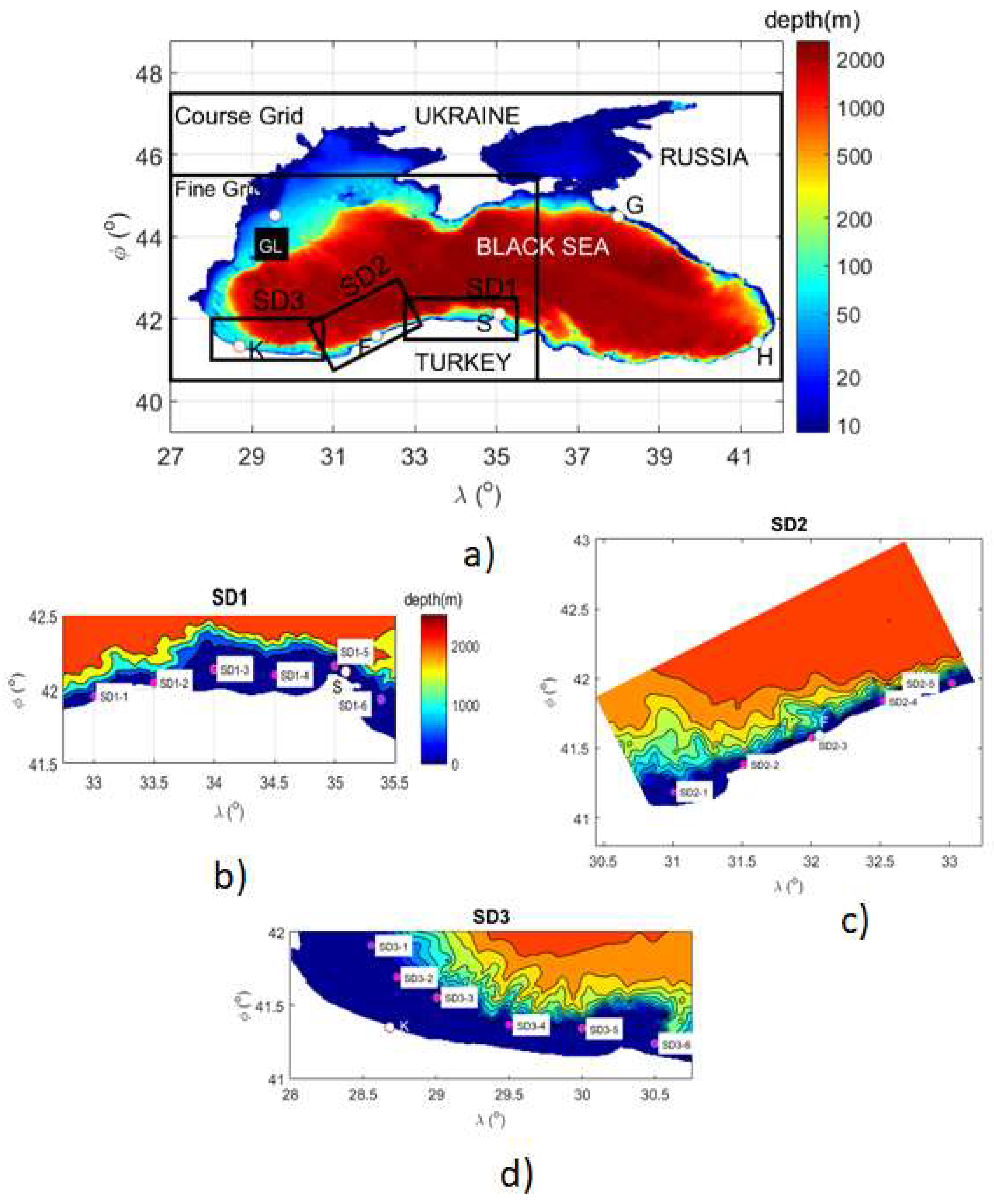
As can be seen from the literature review presented above, the southwestern coasts of the Black Sea can be considered as hotspot areas or high-energy areas (Figure 1). Therefore, in this study, we determined temporal variations of wave energy potential in these hotspot areas using the dataset produced based on a calibrated telescoping nested SWAN model developed by Bingölbali et al. [13].
2. Materials and Methods
The data needed to conduct this study were produced in a project realized by Akpınar et al. [14] whereas Bingölbali et al. [13] presented detailed information on model development, calibration, and validation, as well as initial results. Settings for the calibrated model from which the data used in this study were sourced as follows: Third generation version 41.01AB SWAN model [15] in nonstationary mode and nesting process. Discretization of the directional wave variance density spectrum was conducted with 36 directional bins and 30 frequency bins distributed between 0.04 Hz and 1.0 Hz logarithmically. Based on model development and calibration results in our previous study [13] various wind growth and whitecapping formulation settings were used in each grid for computations of source terms in the model. SWAN model was calibrated based on the whitecapping coefficient in each grid domain using the measurements at the buoy stations remaining in the grid domains. The results ultimately showed that model performance was sensitive to the choice of different wind input and whitecapping formulations and whitecapping coefficient (Cds). Therefore, the model was adjusted based on these formulations and the Cds to give the best prediction performance on each grid. For these parameters, the best performances in the different grid domains were obtained as follows. The Komen [16] formulation for wind input and the Janssen [17,18] formulation for whitecapping with Cds=1.5 were implemented in the coarse domain representing the entire Black Sea. Janssen [17,18] with Cds=3 for both wind input and whitecapping was set in the fine-grid model representing the western Black Sea using boundary conditions from the main domain. Komen [16] for wind and Janssen [17,18] for whitecapping were implemented in the three sub-grids as Cds=3 for SD1 (Sinop), Cds=9 for SD2 (Filyos), and Cds=2 for SD3 (Karaburun) and based on boundary conditions from the fine grid. For sensitivity analysis, the numerical settings of each grid domain (domain size, computational resolutions, frequency resolutions, directional resolutions, frequency ranges, sensitivity to choice of wind fields, etc.) were also individually tested for each grid domain. These tests showed that only the choice of a certain time step leads to improved model performance (lower error and higher correlation). Therefore, in each domain, different time steps were used as shown in Bingölbali et al. [13]. In all grids, in the nesting procedure, all other source terms were kept as the default in our wave model computations because they have no obvious effect. The Discrete Interaction Approximation (DIA) method by Hasselmann et al. [19] was used in the estimation of quadruplet interactions with λ=0.25 and Cnl4=3×10⁷. The value Cfjon=0.038 m2s−3 for bottom friction from following JONSWAP [20] was used following the work by Zijlema et al. [21]. For depth-limited wave breaking, α=1 and γ=0.73 values were adopted following the bore-model of Battjes and Janssen [22]. The Lumped Triad Approximation (LTA) method by Eldeberky [23] was adopted for triad wave-wave interactions modelling.
The Climate Forecast System Reanalysis (CFSR) wind velocity components [24] at 10 m above the water surface, at a time step of 1 h and a spatial resolution of 0.3125° in both latitude and longitude, produced by the National Centers for Environmental Prediction (NCEP) are used as the forcing in the model. The bathymetry, of resolution, is 30 arc seconds in both latitude and longitude, was accessed from the General Bathymetric Chart of the Oceans (GEBCO) [25] database.
Significant wave height (Hm0) and wave energy period (Tm-10) are the fundamental parameters used in the calculation of wave power resource (Pw) in deep water. The wave power (Pw) is given as energy flux per unit of the wave crest length in kW per meter as:
A characteristic mean seawater density () value of 1015 kg/m3 has been chosen for the Black Sea based on spatial and temporal changes affected by salinity and temperature. The wave energy flux per unit crest length, therefore, becomes:
3. Results and Discussion
This section aims to present the results regarding temporal variation of wave energy flux in the hotspot areas of the Black Sea. For this purpose, hourly, monthly, and seasonal variability of the wave energy flux were primarily examined by utilizing the long-term accumulated data for stations (Figure 1) selected at depths of approximately 100 m along the coasts in the three sub-grids SD1, SD2, and SD3. Before presenting the results, some results are here first given regarding the model performance. The detailed results on model development, calibration, and validation can be found in Bingölbali et al. [13]. Model results are evaluated using standard error statistics which include; bias (BIAS), used for the detection of systematic errors, mean absolute error (MAE) used for measuring accuracy of the data, Pearson’s correlation coefficient (r) which estimates variance, the scatter index (SI) which measures relative errors. They are here characterized as follows:
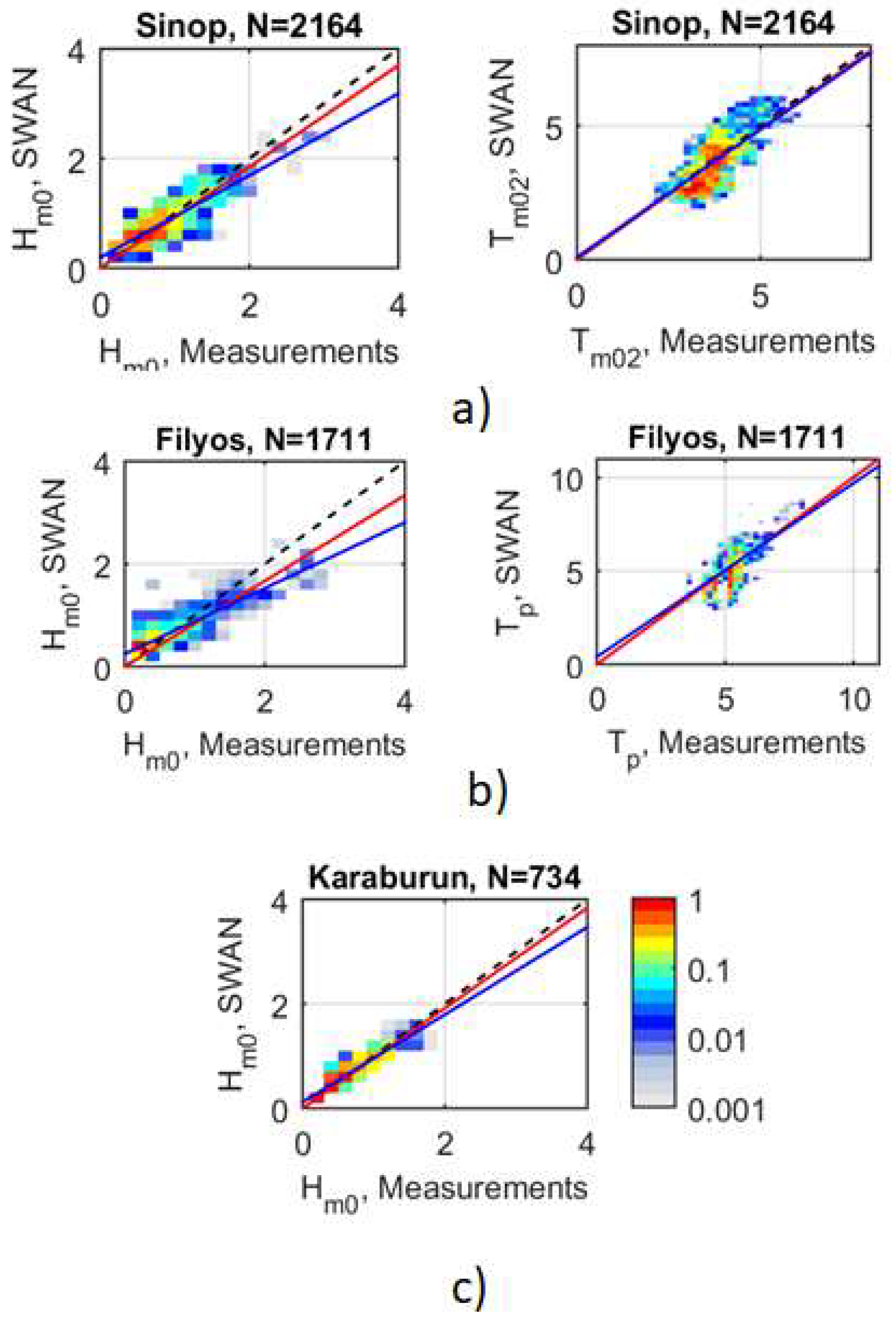
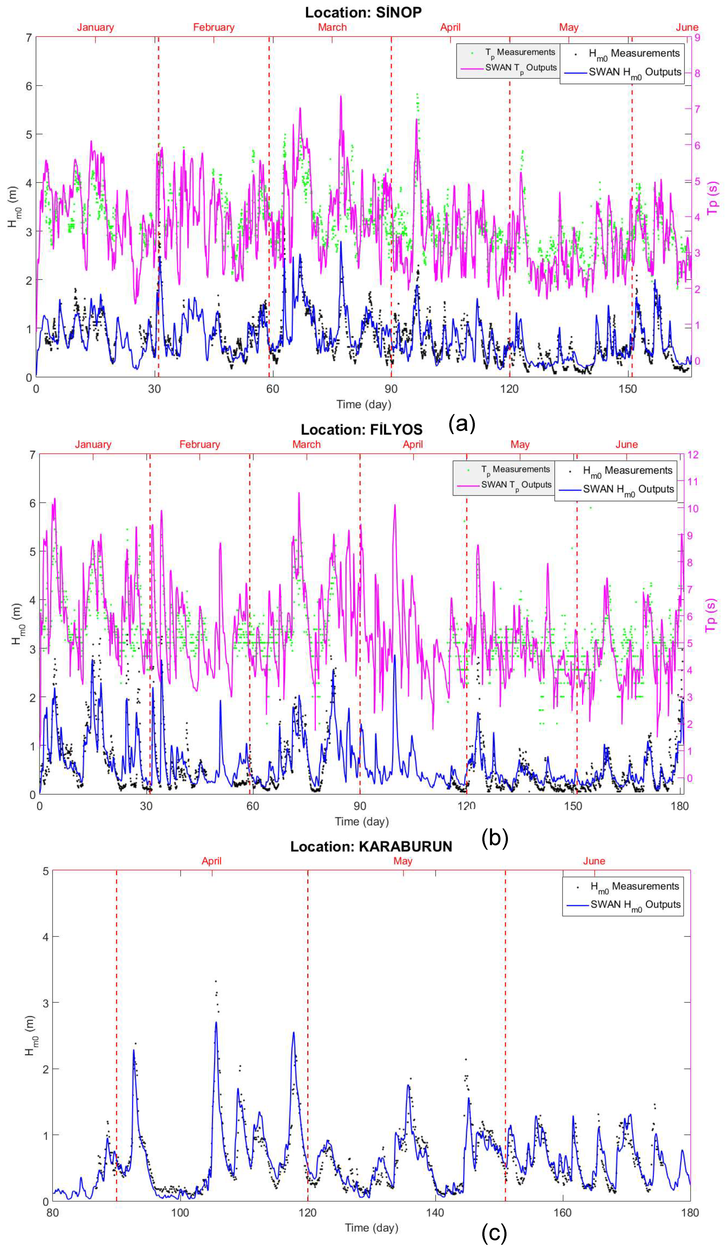
where Oi is the observed value, is the mean value of the observed data, Pi is the predicted value, is the mean value of the predicted data, and N is the total number of data. The error statistics between hindcasts and measurements are given in Table 1. The results show that model results are well in agreement with the measurements in terms of both wave parameters at three buoy locations. Bias varies between 0.01 m and 0.03 m, and the correlation coefficient is about 0.85 for Hm0. At Sinop, bias and correlation coefficient for the mean period are 0.08 s and 0.73. At Filyos, peak period is slightly underestimated. Scatter plots and time series comparison of model hindcasts against the measurements at three buoy locations in the sub-grid domains are also presented in Figure 2 and Figure 3.
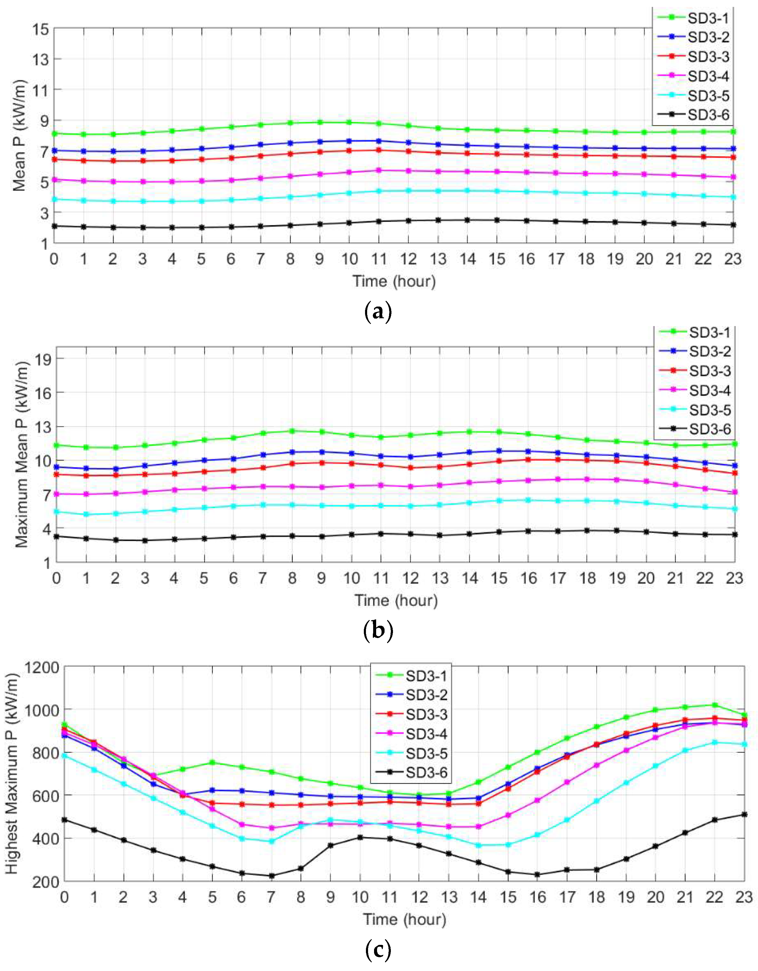
Wave energy flux was determined in the 24 hours of the day for 31 years and also maximum values of each year for 31 years for every 24 hours of the day. Using these maximum values, hourly changes in average highest power and maximum highest power values of each station were determined. Hourly variations of averaged wave power and in average highest power and maximum highest power values based on maximum values of each station for selected stations in sub-grids of Karaburun (SD3), Filyos (SD2), and Sinop (SD1) from 1979 to 2009 are presented in Figure 4, Figure 5 and Figure 6.
According to Figure 4, for the stations in the Karaburun SD3 sub-grid, the fluctuation in the hourly variation of the average wave power is around a maximum of 1 kW/m. This fluctuation, except for station no. 6, has high values in the sub-grid between 07:00 and 14:00. Furthermore, from Figure 4, the average power and average highest power values decrease from the west to the east of the grid. The average power for station 1 and the average highest power are about 8 kW/m and 12 kW/m, and for station 6, 2 kW/m and 4 kW/m, respectively, for all hours. The highest maximum power value is lowest between 03:00 and 15:00 at all stations in this sub-grid except station 6. The highest maximum power value is 1000 kW/m during the 21st and 23rd hours of the day at station 1. The highest maximum power value is 200 kW/m at station 6 and about 400 kW/m at the nearest station 5. These results provide extremely important information for the installation and design of the wave energy conversion systems (WECs) to be established in these regions. WECs can provide an individual energy input for the industrial associations. In addition, WECs can also contribute coastal protection in the areas which are vulnerable to the waves, such as the beach (for example Karaburun, Şile, Karasu, Akçakoca, Kozlu, and Kilimli beaches).
In the Filyos sub-grid, the average power value increases after 07:00 at all stations and declines after 16:00 (Figure 5). The average power shows a decrease from west to east and is higher at station 4 and then station 5. In addition, the average power values of the station 6 in the Karaburun sub-grid are lower than the average power values in station 1 in this grid. However, the average power at all other stations in the Karaburun sub-grid is greater than the average power at all stations in the Filyos sub-grid. In the Filyos, the lowest average power and average highest power value throughout the day are observed at station 3. The highest maximum power is around 550 kW/m at station 1 which is the highest among the other stations. The lowest value of the highest maximum power values is around 200 kW/m in this grid.
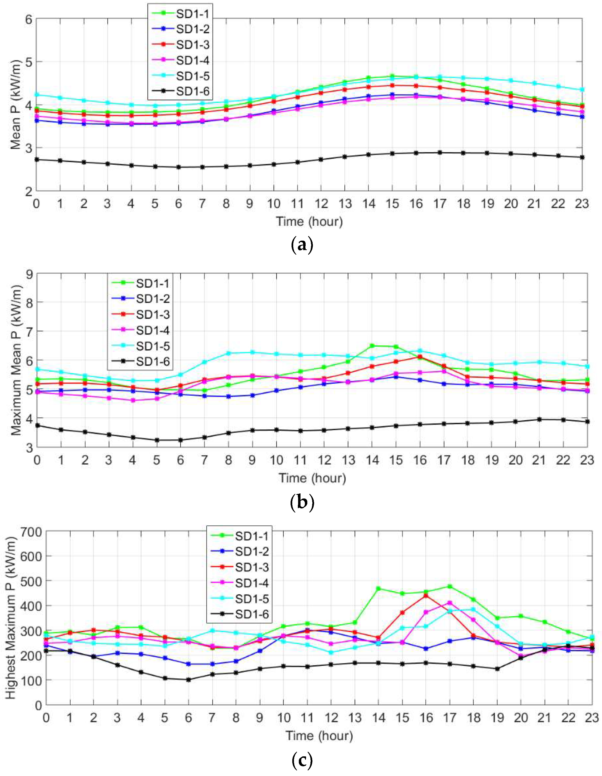
According to Figure 6, in the Sinop sub-grid, the average power, except station 6 is between 3.5 and 4.5 kW/m. The average power at station 6 is between 3 and 2.5 kW/m. All stations consist of a higher average power in the time interval of 10:00 to 19: 00. Sinop stations (excluding station no. 6) offer higher hourly average power than the stations in Filyos and lower values than the Karaburun stations (excluding station no. 6). The average highest power has values in the range of 6.5 to 5 kW/m at all stations except for station 6 whose value is below 4 kW/m. The highest maximum power is about 490 kW/m at station 1 from 14:00 to 17:00. Finally, we can conclude from the results obtained for three sub-grids that there is a higher energy during the day at all stations. In addition, there are a very low fluctuations in mean wave power during the day in the western part while at the eastern stations mean wave energy flux shows higher fluctuations.
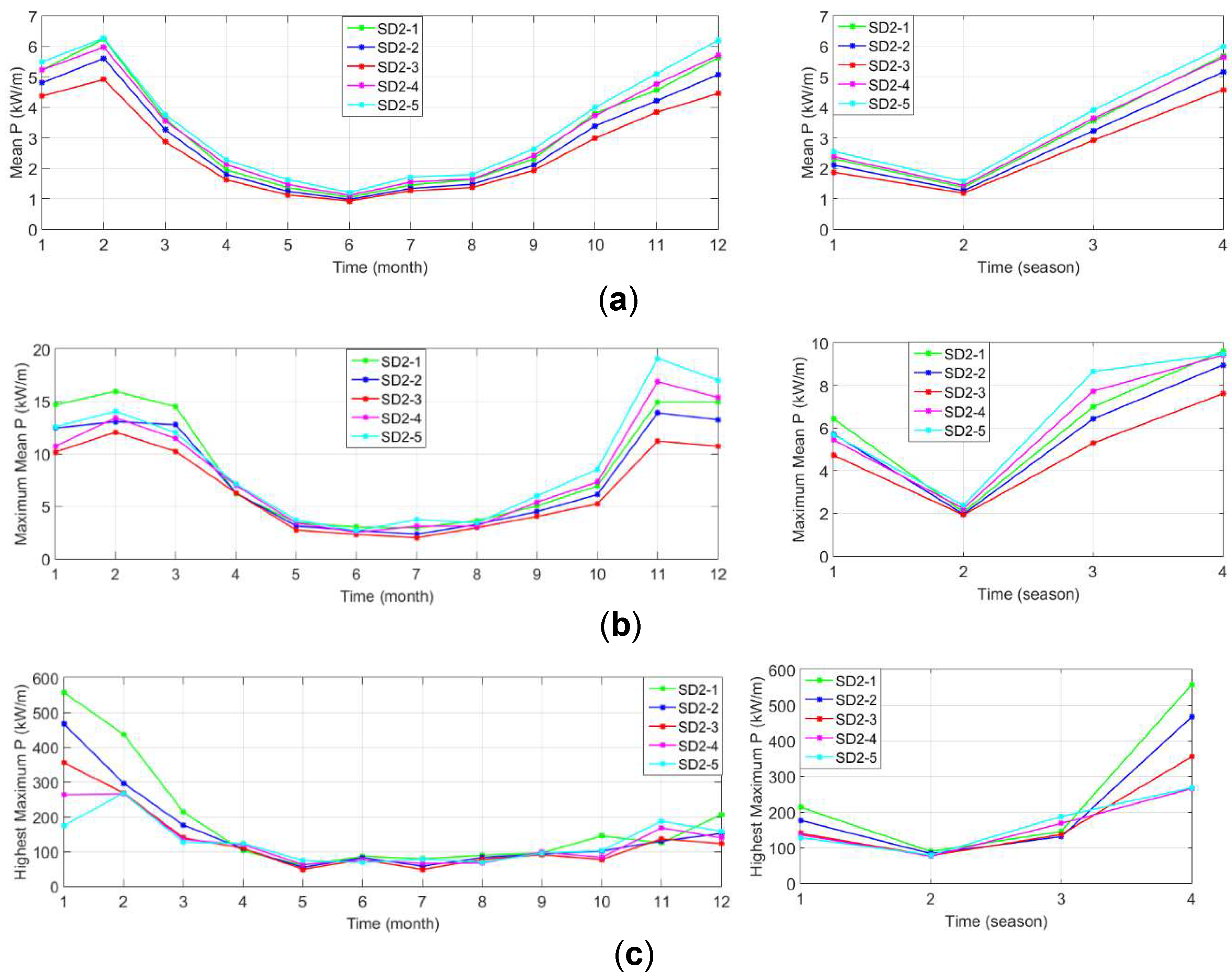
After examining the hourly variations of the wave power, monthly, and seasonal average power, average highest power and the highest maximum power values were determined for each station in each sub-grid. After that, monthly and seasonal variations of these values were also examined. Their graphical comparisons are presented in Figure 7, Figure 8 and Figure 9. As can be seen from Figure 7, in the Karaburun sub-grid, the average wave power is lowest at all stations in summer months (May, June, and July), while it is the highest in winter months (December, January, and February). In the monthly and seasonal variations of the average wave power, it is seen that the average power decreases from the west to the east of the sub-grid. The highest average power is 18 kW/m at station 1 in December and 16 kW/m in the winter, and the lowest average power at station 6 in April to July and in summer is less than 1 kW/m. Monthly and seasonal variation of average highest power has similarities to that of the average wave power at the stations. The largest value of the average highest power at station 1 is about 65 kW/m in December, while the lowest value is very close to zero at station 6 in May to July. In addition, the average highest power value is around 28 kW/m at station 1 in winter compared with the other stations, while this value is very close to zero in summer at station 6. The maximum value of the highest maximum power in the Karaburun sub-grid was obtained at approximately 1050 kW/m in January at station 1. Highest values of this parameter were obtained at all stations in winter (1000 kW/m station 1 and 550 kW/m station 6), while the lowest in summer (200 kW/m station 1 and 100 kW/m station 6).
The monthly variations of the mean power in Filyos sub-grid (Figure 8) show that the average power values obtained at all stations in spring and summer months are very close to each other. Moreover, a difference of maximum 2 kW/m in the average wave power among the stations in autumn and winter months is observed. The average power is approximately 1.5 kW/m, 2.1 kW/m, 3.3 kW/m, and 5 kW/m, respectively, in the summer, spring, autumn, and winter seasons at all stations and in the months representing these seasons. Here, the monthly and seasonal average wave power values are very close to each other in this sub-grid. In addition, the average highest power and highest maximum power values of all stations in this grid are very close to each other. The average highest power is approximately 3 kW/m at all stations in May to August, and approximately 5.5 kW/m in April, September, and October, and approximately 12.5 kW/m in the other months. The highest maximum power is 100 kW/m in April to October and 150 kW/m in March, November, and December at all stations in this grid. In addition, in January and February, an average value of 350 kW/m for the highest maximum wave power is present at all stations. A maximum value of approximately 580 kW/m is observed at station 1 while a minimum value of 196 kW/m occurs at station 5. The maximum value for the highest maximum wave power is approximately 550 kW/m in winter at station 1 while the lowest value of 260 kW/m is observed at stations 4 and 5.
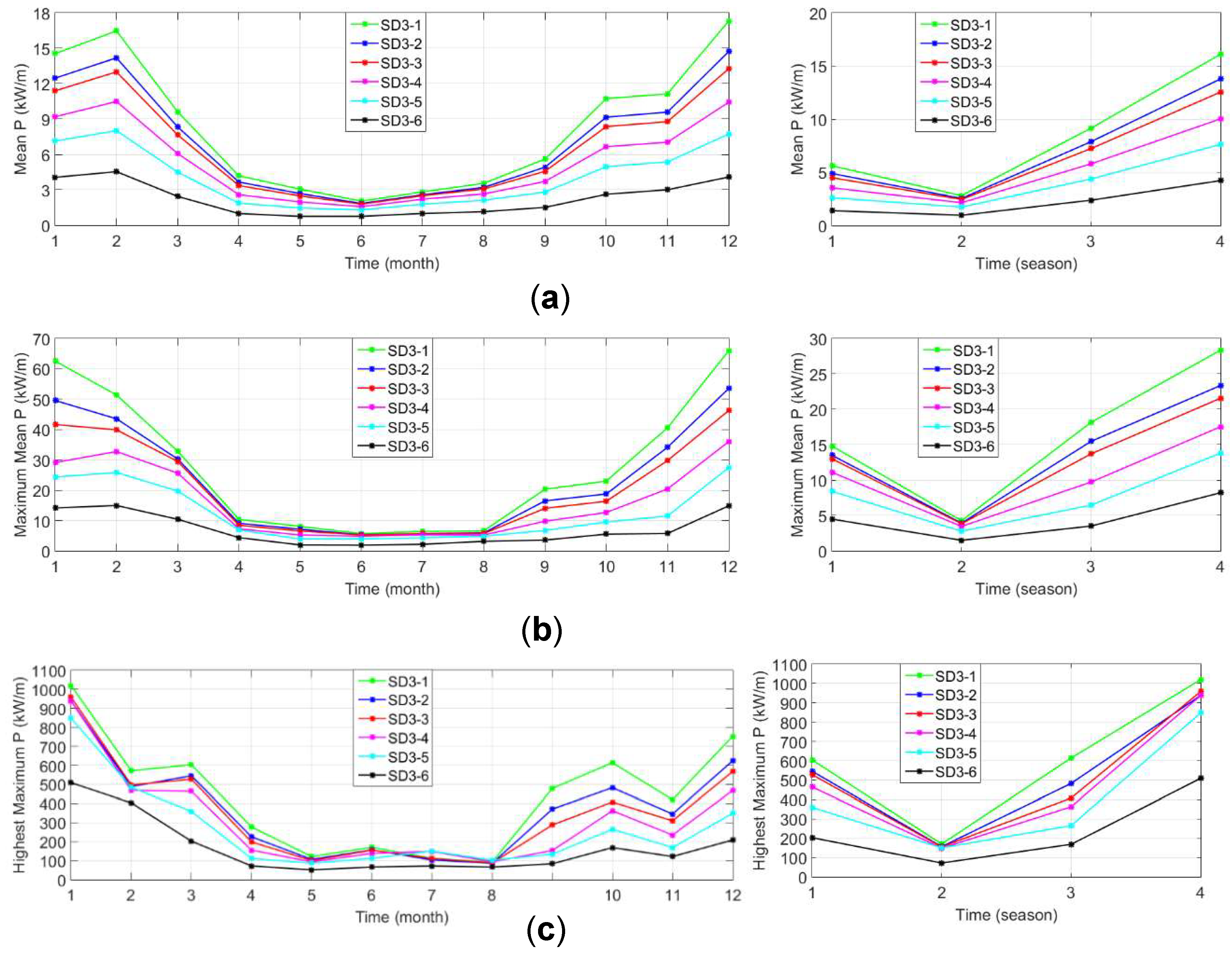
The average wave power determined for the six stations of the Sinop (SD1) sub-grid between 1979 and 2009 and the monthly and seasonal variations of the average highest power and the highest maximum values based on the maximum wave power values of each year are presented in Figure 9. According to these findings, monthly and seasonal average and average highest wave powers are very close to each other except for station 6. The average wave power and average highest wave power have the highest values at all stations during the winter season and in the months representing this season, followed by autumn, spring, and summer and months representing these seasons. The average wave power at all stations (except station 6) is around 2 kW/m in the summer and during the months representing it and around 7 kW/m in winter and in the months representing it. A value of 500 kW/m of the highest maximum power is observed at station 1 in the October and February, which is the largest compared to the monthly values of the other stations.
The variations in the annual maximum and average wave power and their linear trends are determined by the using long-term data generated at the selected stations for each sub-grid between 1979 and 2009 and are presented in Figure 10, Figure 11 and Figure 12. Using the long-term data set produced for all selected stations, an ideal line was drawn for only yearly maximum and average values and the direction of the trend (positive or negative) is determined from the inclination of this line. The data were not subjected to any trend testing. Therefore, the trends determined here may not be significant.
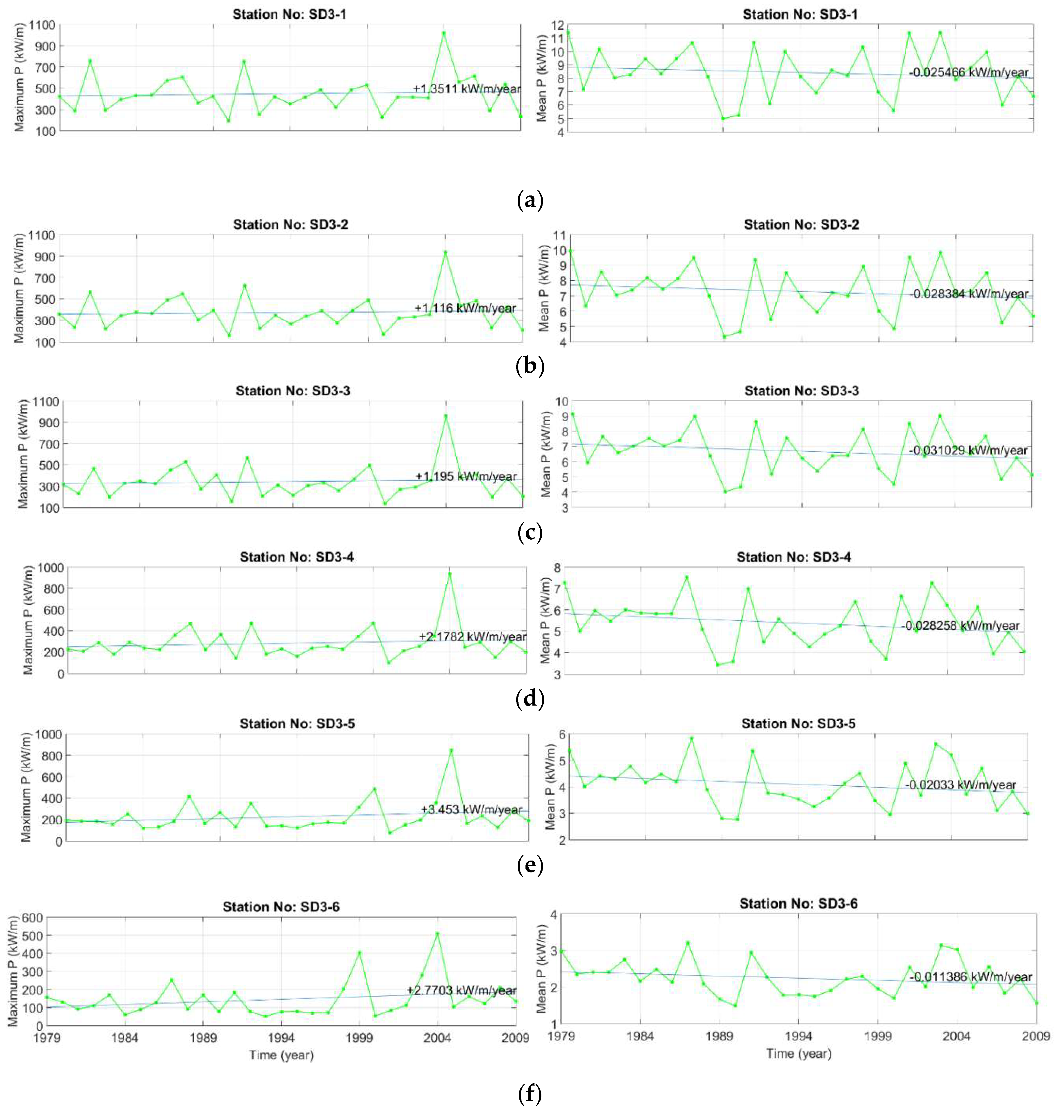
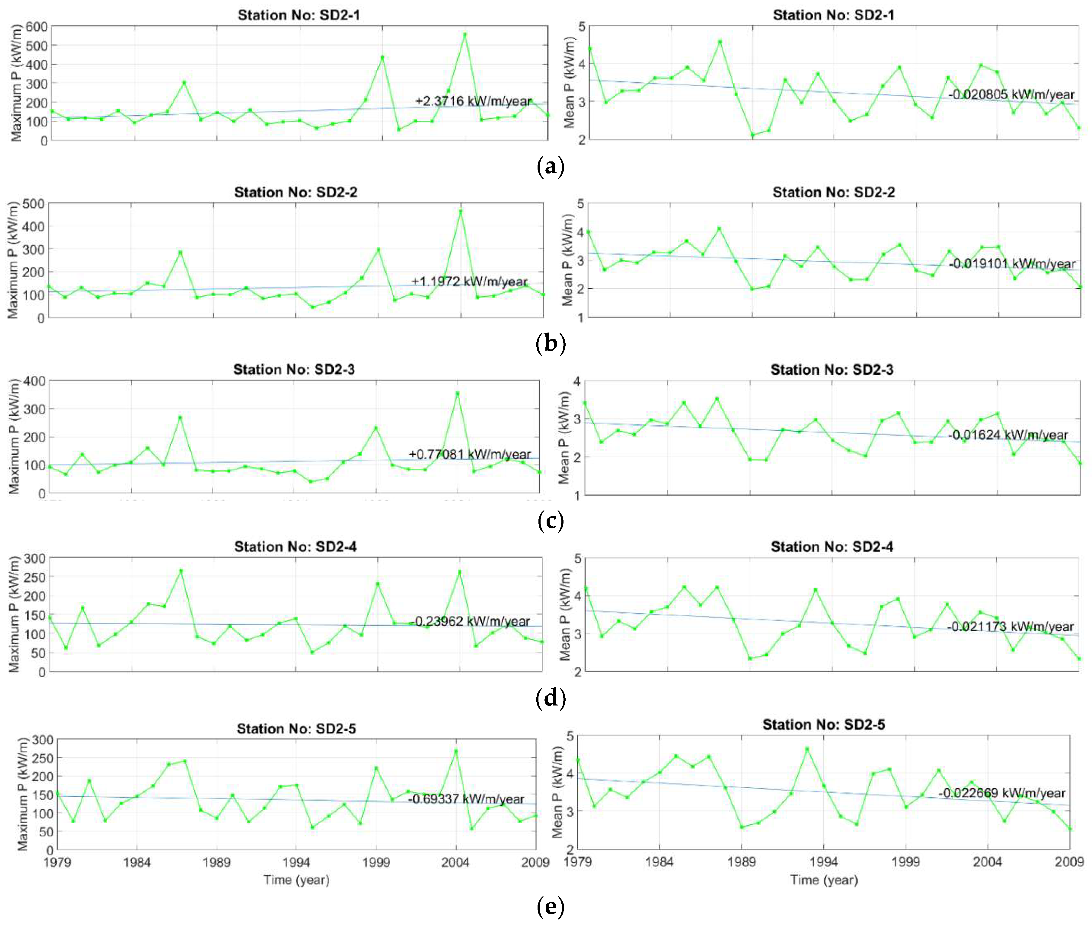
All stations in the Karaburun sub-grid have an increasing trend for yearly maximum power, while a negative (decreasing) trend is observed for the average power (Figure 10). The highest trend for the yearly maximum power is found at station 5 with +1.345 kW/m/year, while the lowest trend is observed at station 2 with +1.116 kW/m/year. For the annual average power, the lowest trend is 0.01 kW/m/year at station 6, followed by −0.02 kW/m/year at station 5 and the other stations have approximately −0.03 kW/m/year. Furthermore, it is observed that the maximum annual power has peaked at all stations in 2004. While the yearly average power variation range is 6.5 kW/m/year at the stations west of the sub-grid, it decreases to 2 kW/m/year at the eastern stations. Although there is a lower annual average wave power at the stations to the east of this sub-grid, it shows that there is an average annual wave power in a narrower strip. It is observed that there is a higher variation interval at the stations with higher annual average wave power. As seen in Figure 11, the annual maximum wave power at all stations, except for stations 4 and 5, is in an increasing trend and decreases at stations 4 and 5. There is a decreasing trend at all stations in the variation of the annual average wave power. For the yearly maximum wave power, the highest increasing trend is +2.37 kW/m/year at station 1 and a downward trend of −0.69 kW/m/year at station 5. For the annual average wave power, there has been a decreasing trend of approximately −0.02 kW/m/year at all stations. The year in which the maximum annual power value is greatest is determined as 2004 at all stations. Variations in the annual average power have generally shown a similar trend at all stations in this sub-grid.
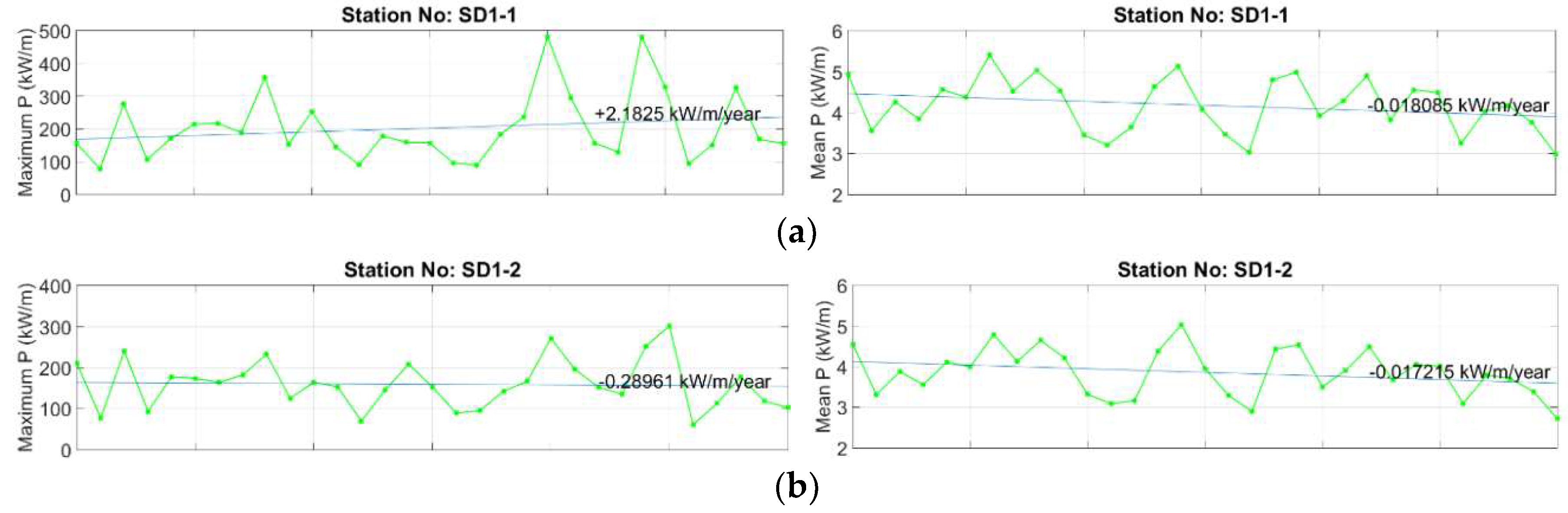
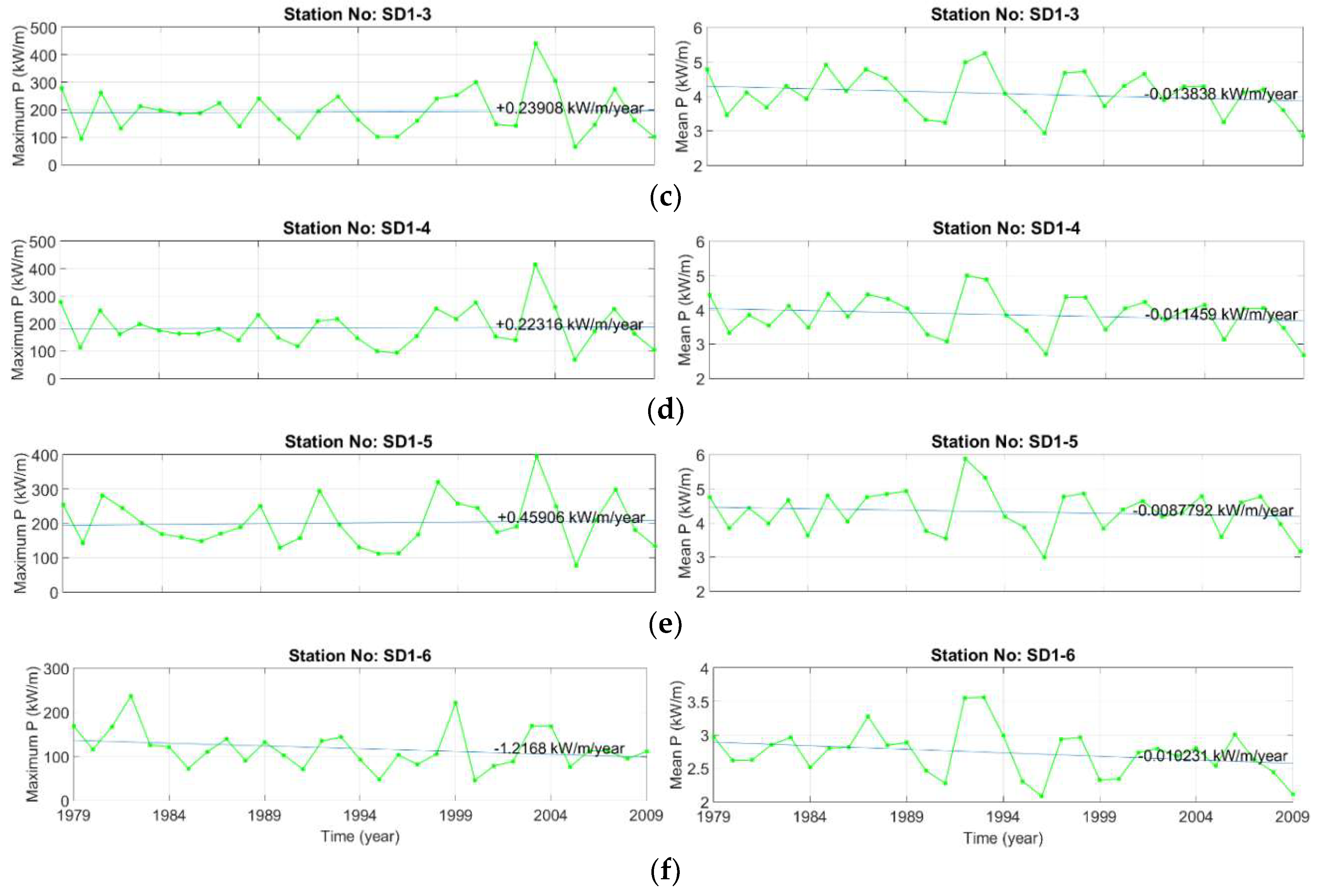
Figure 12 shows variations and linear trends of the annual maximum and average wave power defined for the 6 stations of the Sinop (SD1) sub-grid. Here, the annual maximum power tends to decrease at stations 2 and 6, while an increasing trend is observed at the other stations. The highest increase is 2.18 kW/m/year observed in station 1, and the highest decreasing trend is 1.22 kW/m/year observed at station 6. Based on annual variations in the annual average power, there is a decreasing trend at all stations. At stations 1 and 2, the average annual power has a decreasing trend of about 0.02, while at the other stations approximately 0.01 is encountered. There is a change from 50 to 500 kW/m/year in the annual maximum power at stations 1, 3, and 4 representing a fluctuation of about 400 kW/m/year. This fluctuation is approximately 350 kW/m/year, from 50 to 400 kW/m/year, at station 5; 250 kW/m/year, between 50 and 300 kW/m/year, at station 2, and 200 kW/m/year, between 50 and 250 kW/m/year, at station 6. In the case of average power, a fluctuation of about 2.5 kW/m/year, varying from 2.5 to 5.5 kW/m/year, is observed at stations 1, 2, and 4. 3.5 kilowatts per meter per year, between 2.5 to 6 kW/m/year, at stations 3 and 5, and approximately 1.5 kW/m/year between 2 and 3.5 kW/m/year at station 6.
Since the main target of the present work is to study the variability of the wave flux in some hotspot areas of the Black Sea, its results also have some direct industrial applications related to the extraction of the marine energy especially. Furthermore, this extraction of the marine energy might have also useful applications as regards the coastal protection, which represents a very important environmental issue in the Black Sea (see for example [26,27,28]).
4. Conclusion
In this study, long term temporal variation of wave energy flux in the high-energy potential areas of the Black Sea was discussed on the basis of yearly, seasonal, monthly, and hourly scales. With a three-layered nested modelling system, a 31-year long-term wave dataset was produced and, thus, wave energy potential variations were estimated using this high-resolution and accurate dataset. In this study, the model performance assessment is first given, and then model outputs are evaluated. The accuracy of the model results emerged with time series and scatter diagrams and error statistics of the significant wave heights and wave periods, visually and numerically. Evaluation of the model results deals with long-term variations of averaged and maximum wave power in an hourly, monthly, seasonal, and annual basis. The results show that model results are well in agreement with the measurements in terms of both wave parameters. There is a higher energy during the day at all stations. In addition, there are a very low fluctuations (max 1 kW/m) in mean wave power during the day. Variation in mean wave power is lower in the summer months while in the winter months the stations have higher differences in wave power. Furthermore, a decreasing trend in mean wave energy flux at all stations but an increasing trend in maximum wave power at most of the stations were found. Finally, of note, the results presented in the present work are in line with those from various studies targeting the basin of the Black Sea [4,11,29,30].
Author Contributions
The idea of the proposed paper and the first draft belong to A.A. H.J. processed the data and designed the figures. E.R. performed an analysis of the results and the supervision of the work. All authors agreed with the final content.
Funding
This research was funded by The Scientific and Technological Research Council of Turkey (TUBITAK), grant number 214M436.
Acknowledgments
The work of the corresponding author is performed in the framework of the research project REMARC (Renewable Energy extraction in MARine environment and its Coastal impact) granted by the Romanian Executive Agency for Higher Education, Research, Development and Innovation Funding–UEFISCDI, grant number PN-III-P4-IDPCE-2016-0017. The authors would like to thank the Turkish Ministry of Transport (General Directorate of Railwsays, Ports and Airports Construction) which provided us with wave measurements at Filyos and Karaburun. We also express our appreciation to Erdal Özhan (Director of the NATO TU-WAVES) from Middle East Technical University, Ankara, Turkey, who supplied measurement data of Sinop, as well as the NATO Science for Stability Program, supporter of the NATO TU-WAVES project.
Conflicts of Interest
The authors declare no conflict of interest.
References
- Panicker, N.N. Power resource potential of ocean surface wave. In Proceedings of the Wave and Salinity Gradient Workshop, Newark, DE, USA, 24 May 1976; pp. J1–J48. [Google Scholar]
- Leijon, M.; Bernhoff, H.; Berg, M.; Ågren, O. Economical considerations of renewable electric energy production-especially development of wave energy. Renew Energy 2003, 8, 1201–1209. [Google Scholar] [CrossRef]
- Kamranzad, B.; Etemad-Shahidi, A.; Chegini, V. Sustainability of wave energy resources in southern Caspian Sea. Energy 2016, 97, 549–559. [Google Scholar] [CrossRef]
- Rusu, E. Wave energy assessments in the Black Sea. J. Mar. Sci. Technol. 2009, 14, 359–372. [Google Scholar] [CrossRef]
- Akpınar, A.; Kömürcü, M.I. Wave energy potential along the south-east coasts of the Black Sea. Energy 2012, 42, 289–302. [Google Scholar] [CrossRef]
- Akpınar, A.; Kömürcü, M.I. Assessment of wave energy resource of the Black Sea based on 15-year numerical hindcast data. Appl. Energy 2013, 101, 502–512. [Google Scholar] [CrossRef]
- Aydoğan, B.; Ayat Aydoğan, B.; Yüksel, Y. Black Sea wave energy atlas from 13 years hindcasted wave data. Renew. Energy 2013, 57, 436–447. [Google Scholar] [CrossRef]
- Divinsky, B.V.; Kosyan, R.D. Spatiotemporal variability of the Black Sea wave climate in the last 37 years. Cont. Shelf Res. 2017, 136, 1–19. [Google Scholar] [CrossRef]
- Galabov, V. The Black Sea Wave Energy: The Present State and the Twentieth Century Changes. Available online: https://arxiv.org/pdf/1507.01187.pdf (accessed on 20 September 2018).
- Akpınar, A.; Bingölbali, B.; Van Vledder, G.Ph. Long-term analysis of wave power potential in the Black Sea, based on 31-year SWAN simulations. Ocean Eng. 2017, 130, 482–497. [Google Scholar] [CrossRef]
- Rusu, L. Assessment of the wave energy in the Black Sea based on a 15-year hindcast with data assimilation. Energies 2015, 8, 10370–10388. [Google Scholar] [CrossRef]
- Saprykina, Y.; Kuznetsov, S. Analysis of the variability of wave energy due to climate changes on the example of the Black Sea. Energies 2018, 11, 2020. [Google Scholar] [CrossRef]
- Bingölbali, B.; Akpınar, A.; Jafali, H.; Van Vledder, G.Ph. Downscaling of wave climate in the western Black Sea. Ocean Eng. 2019, 172, 31–45. [Google Scholar] [CrossRef]
- Akpınar, A.; Bekiroğlu, S.; Van Vledder, G.Ph.; Bingölbali, B.; Jafali, H. Temporal and Spatial Analysis of Wave Energy Potential during Southwestern Coasts of the Black Sea, TUBITAK Project; 2015–2017.
- Booij, N.; Holthuijsen, L.H.; Ris, R.C. A third-generation wave model for coastal regions. 1: Model description and validation. J. Geophys. Res. 1999, 104, 7649–7666. [Google Scholar] [CrossRef]
- Komen, G.J.; Cavaleri, L.; Donelan, M.; Hasselmann, K.; Hasselmann, S.; Janssen, P.A.E.M. Dynamics and Modelling of Ocean Waves; Cambridge University Press: Cambridge, UK, 1994. [Google Scholar]
- Janssen, P.A.E.M. Wave induced stress and the drag of air flow over sea water. J. Phys. Oceanogr. 1989, 19, 745–754. [Google Scholar] [CrossRef]
- Janssen, P.A.E.M. Quasi-linear theory of wind-wave generation applied to wave forecasting. J. Phys. Oceanogr. 1991, 21, 1631–1642. [Google Scholar] [CrossRef]
- Hasselmann, S.; Hasselmann, K.; Allender, J.H.; Barnett, T.P. Computations and parameterizations of the linear energy transfer in a gravity wave spectrum, Part II: Parameterizations of the nonlinear transfer for application in wave models. J. Phys. Oceanogr. 1985, 15, 1378–1391. [Google Scholar] [CrossRef]
- Hasselmann, K.; Barnett, T.P.; Bouws, E.; Carlson, H.; Cartwright, D.E.; Enke, K.; Ewing, J.A.; Gienapp, H.; Hasselmann, D.E.; Kruseman, P.; et al. Measurements of wind-wave growth and swell decay during the joint North Sea wave project (JONSWAP). Dtsch. Hydrogr. Z. Suppl. 1973, 12, A8. [Google Scholar]
- Zijlema, M.; Van Vledder, G.P.; Holthuijsen, L.H. Bottom friction and wind drag for wave models. Coast Eng. 2012, 65, 19–26. [Google Scholar] [CrossRef]
- Battjes, J.A.; Janssen, J.P.F.M. Energy loss and set-up due to breaking of random waves. In Proceedings of the 16th International Conference on Coastal Engineering, Hamburg, Germany, 27 August–3 September 1978. [Google Scholar]
- Eldeberky, Y. Nonlinear Transformation of Wave Spectra in the Nearshore Zone. Ph.D. Thesis, Delft University of Technology, Delft, The Netherlands, 1996. [Google Scholar]
- Saha, S.; Moorthi, S.; Pan, H.-L.; Wu, X.; Wang, J.; Nadigai, S.; Tripp, P.; Kistler, R.; Woollen, J.; Behringer, D.; et al. The NCEP climate forecast system reanalysis. Bull. Am. Meteorol. Soc. 2010, 91, 1015–1057. [Google Scholar] [CrossRef]
- GEBCO. British Oceanographic Data Centre, Centenary Edition of the GEBCO Digital Atlas [CDROM]; Behalf of the Intergovernmental Oceanographic Commission and the International Hydrographic Organization: Liverpool, UK, 2014. [Google Scholar]
- Diaconu, S.; Rusu, E. The Environmental Impact of a Wave Dragon Array Operating in the Black Sea. Sci. World J. 2013, 2013, 498013. [Google Scholar] [CrossRef]
- Zanopol, A.T.; Onea, F.; Rusu, E. Evaluation of the Coastal Influence of a Generic Wave Farm Operating in the Romanian Nearshore. J. Environ. Prot. Ecol. 2014, 15, 597–605. [Google Scholar]
- Rusu, E. Analysis of the Effect of a Marine Energy Farm to Protect a Biosphere Reserve. In Proceedings of the 3rd International Conference on Chemical and Food Engineering, Tokyo, Japan, 13–15 April 2016. [Google Scholar]
- Lin-Ye, J.; Garcia-Leon, M.; Gracia, V.; Ortego, M.I.; Stanica, A.; Sanchez-Arcilla, A. Multivariate Hybrid Modelling of Future Wave-Storms at the Northwestern Black Sea. Water 2018, 10, 221. [Google Scholar] [CrossRef]
- Onea, F.; Rusu, L. A Long-Term Assessment of the Black Sea Wave Climate. Sustainability 2017, 9, 1875. [Google Scholar] [CrossRef]
Figure 1.
(a) Map of the Black Sea. The computational domain for the Simulating Waves Nearshore (SWAN) model is enclosed by the black rectangles (the nested grids). The outermost black rectangle represents the computational coarse domain. Inner black rectangle shows the boundaries of the finer grid and the innermost black rectangles are presented as the sub-grid domains SD1, SD2, and SD3; (b) Mab of the sub-grid domain SD1; (c) Mab of the sub-grid domain SD2; (d) Mab of the sub-grid domain SD3. The measurements in white points are used in the model development, calibration, and validation. The letters GL, G, H, S, F, and K refer Gloria, Gelendzhik, Hopa, Sinop, Filyos, and Karaburun buoy locations, respectively. The positions of the stations selected in three sub-domains are shown by pink circles and color bars and color maps present bathymetries for the entire Black Sea and three sub-grids. φ and λ represent latitudes and longitudes.

Figure 2.
Scatter plots between model hindcasts and the measurements at three buoy locations in the sub-grid domains. The data for the first six months of 1996 and 1995 at (a) Sinop and (b) Filyos buoy locations in SD1 and SD2 sub-grid domains, respectively, and between March and June 2004 at (c) Karaburun in SD3 sub-grid domain is used. The color scheme in scatter diagrams represents the log10 of the number of entries in a square box of 0.2 m and 0.2 s for Hm0 and Tp and Tm02, respectively, normalized with the log10 of the maximum number of entries in a box. In this way, the clustering of data points is highlighted. Each figure contains three lines. The solid blue line is the linear regression line according to the model y = a + bx, the red line according to the model y = cx and the line of perfect agreement is the dashed line. The number of samples N and the names of the buoy locations are shown in the title and in the plot.

Figure 3.
Time series comparison of model hindcasts against the measurements at three buoy locations in the sub-grid domains. The data for the first six months of 1996 and 1995 at (a) Sinop and (b) Filyos buoy locations in SD1 and SD2 sub-grid domains, respectively, and between March and June 2004 at (c) Karaburun in SD3 sub-grid domain is used. The names of the buoy locations are shown in the title.

Figure 4.
(a) Long-term hourly variations during the day for average wave power, (b) average maximum power and (c) the highest maximum power values determined depending on values of maximum wave power for each year for the period 1979 to 2009 at the selected locations in SD3 (Karaburun) sub-domain.
Figure 4.
(a) Long-term hourly variations during the day for average wave power, (b) average maximum power and (c) the highest maximum power values determined depending on values of maximum wave power for each year for the period 1979 to 2009 at the selected locations in SD3 (Karaburun) sub-domain.

Figure 5.
(a) Long-term hourly variations during the day for average wave power, (b) average maximum power and (c) the highest maximum power values determined depending on values of maximum wave power for each year for the period 1979 to 2009 at the selected locations in SD2 (Filyos) sub-domain.
Figure 5.
(a) Long-term hourly variations during the day for average wave power, (b) average maximum power and (c) the highest maximum power values determined depending on values of maximum wave power for each year for the period 1979 to 2009 at the selected locations in SD2 (Filyos) sub-domain.

Figure 6.
(a) Long-term hourly variations during the day for average wave power, (b) average maximum power and (c) the highest maximum power c) values determined depending on values of maximum wave power for each year for the period 1979 to 2009 at the selected locations in SD1 (Sinop) sub-domain.
Figure 6.
(a) Long-term hourly variations during the day for average wave power, (b) average maximum power and (c) the highest maximum power c) values determined depending on values of maximum wave power for each year for the period 1979 to 2009 at the selected locations in SD1 (Sinop) sub-domain.

Figure 7.
(a) Monthly and seasonal variations for average wave power, (b) average maximum power and (c) the highest maximum power values determined depending on values of maximum wave power for each year for the period 1979 to 2009 at the selected locations in SD3 (Karaburun) sub-domain. In the subplots, indicating the seasonal variations (from the right side), 1 indicates Spring, 2- Summer, 3- Autumn and 4- Winter.

Figure 8.
(a) Monthly and seasonal variations for average wave power, (b) average maximum power and (c) the highest maximum power (c) values determined depending on values of maximum wave power for each year for the period 1979 to 2009 at the selected locations in SD2 (Filyos) sub-domain. In the subplots, indicating the seasonal variations (from the right side), 1 indicates Spring, 2- Summer, 3- Autumn and 4- Winter.

Figure 9.
(a) Monthly and seasonal variations for average wave power, (b) average maximum power and (c) the highest maximum power (c) values determined depending on values of maximum wave power for each year for the period 1979 to 2009 at the selected locations in SD1 (Sinop) sub-domain. In the subplots, indicating the seasonal variations (from the right side), 1 indicates Spring, 2- Summer, 3- Autumn and 4- Winter.

Figure 10.
Annual maximum and average wave power variations and linear trends for selected stations in Karaburun SD3 sub-domain for the years 1979 to 2009. (a) station SD3-1; (b) station SD3-2; (c) station SD3-3; (d) station SD3-4; (e) station SD3-5; (f) station SD3-6.
Figure 10.
Annual maximum and average wave power variations and linear trends for selected stations in Karaburun SD3 sub-domain for the years 1979 to 2009. (a) station SD3-1; (b) station SD3-2; (c) station SD3-3; (d) station SD3-4; (e) station SD3-5; (f) station SD3-6.

Figure 11.
Annual maximum and average wave power variations and linear trends for selected stations in Filyos SD2 sub-domain for the years 1979 to 2009. (a) station SD2-1; (b) station SD2-2; (c) station SD2-3; (d) station SD2-4; (e) station SD2-5.
Figure 11.
Annual maximum and average wave power variations and linear trends for selected stations in Filyos SD2 sub-domain for the years 1979 to 2009. (a) station SD2-1; (b) station SD2-2; (c) station SD2-3; (d) station SD2-4; (e) station SD2-5.

Figure 12.
Annual maximum and average wave power variations and linear trends for selected stations in Sinop SD1 domain for the years 1979 to 2009. (a) station SD1-1; (b) station SD1-2; (c) station SD1-3; (d) station SD1-4; (e) station SD1-5; (f) station SD1-6.
Figure 12.
Annual maximum and average wave power variations and linear trends for selected stations in Sinop SD1 domain for the years 1979 to 2009. (a) station SD1-1; (b) station SD1-2; (c) station SD1-3; (d) station SD1-4; (e) station SD1-5; (f) station SD1-6.


Table 1.
The error statistics between model hindcasts and measurements at three buoy locations.
| Locations | BIAS | MAE | SI | r | |
|---|---|---|---|---|---|
| Sinop | Hm0 (m) | 0.01 | 0.20 | 0.34 | 0.84 |
| Filyos | −0.03 | 0.24 | 0.58 | 0.85 | |
| Karaburun | −0.01 | 0.15 | 0.34 | 0.88 | |
| Sinop | Tm02 (s) | 0.08 | 0.59 | 0.19 | 0.73 |
| Filyos | Tp (s) | −0.03 | 0.88 | 0.22 | 0.68 |
© 2019 by the authors. Licensee MDPI, Basel, Switzerland. This article is an open access article distributed under the terms and conditions of the Creative Commons Attribution (CC BY) license (http://creativecommons.org/licenses/by/4.0/).
Share and Cite
MDPI and ACS Style
Akpınar, A.; Jafali, H.; Rusu, E. Temporal Variation of the Wave Energy Flux in Hotspot Areas of the Black Sea. Sustainability 2019, 11, 562. https://doi.org/10.3390/su11030562
AMA Style
Akpınar A, Jafali H, Rusu E. Temporal Variation of the Wave Energy Flux in Hotspot Areas of the Black Sea. Sustainability. 2019; 11(3):562. https://doi.org/10.3390/su11030562
Chicago/Turabian StyleAkpınar, Adem, Halid Jafali, and Eugen Rusu. 2019. "Temporal Variation of the Wave Energy Flux in Hotspot Areas of the Black Sea" Sustainability 11, no. 3: 562. https://doi.org/10.3390/su11030562
Note that from the first issue of 2016, this journal uses article numbers instead of page numbers. See further details here.