A Study of the Socioeconomic Factors Influencing Migration in Russia

Abstract

Russia has experienced population decline in years and the economic development in Russia is largely restricted by labor shortage, particularly for the Far North and East region. In order to explore the migration mechanisms, six socioeconomic factors were selected to explore the influences on the net migration. Data from the 82 regions covering four time periods (2000, 2005, 2010 and 2015) was processed use spatial panel econometric analysis and the time-period fixed effects Spatial Durbin Model (SDM) was selected as the best fit model after tests. The results indicates that, unemployment and infant death rate are significantly negatively associated with net migration, while urbanization rate, urban scale and life expectancy are significantly positively associated with net migration; every 100 USD increase in per capita GRP (Gross Regional Product) is positively related with averagely 5.4 net migrates in the region; every 1 year increase in life expectancy would increase 1052 net migrates; every 1sqm increase in urban scale would increase the net migrates by 11.75 and every 1% increase in unemployment would lead to a decrease of 0.54 net migrates. Spillover effect was also found for per capita GRP and life expectancy, indicating that the increase of per capita GRP and life expectancy in neighboring regions can also increase the attractiveness in one region. It can be concluded that better job market, better economic status and health related wellbeing are all attracting factors for migrates and these factors can even make the neighborhood region more attractive for immigrates. Considering the ambitious development plan for the Russia Far North and East regions, related suggestions on attracting migrates are provided.

1. Introduction

It is well-known that labor shortage in Russia is constraining the regional development of the whole country, most significantly in the Arctic and Far North and East [1,2]. A solid support in terms of human resources is needed for the regional development. The Russia population has experienced population loss since the end of the Soviet Union, even with a boom of significant influx migration (fluctuation) because of the collapse of the Soviet Union in the 1990s, with driving forces like repatriation, religion, wars, related migration policies or education [3,4]. This somehow alleviated the population loss but has not stopped the trend. The repatriation migration between Russia and the former Soviet republics slowed down since 2000 [5]. Unlike the “repatriation” or “ethnic return” dominated migration pattern in the 1990s right after the collapse of Soviet Union, in connection with the stabilization of the social and economic situation, the major types of migration in Russia after the 2000s, are labor migration (economic reason) or education or the combination (stay in the place after education) and the majority of the migration population are young population less than 45 years old [6].

In the Far North and East, due to the stop of the strategic distribution of labor to these regions in around 2000, the labors were free to move without any attracting subsidy like before, which resulted in a huge outflow of people from the remote Far North regions [7]. However, the use of natural resources including mining, oil and gas exploitation, where the Far North and East is abundant, became increasingly important for economic development, particularly when the international oil and gas price shooting up since the 1999. This made the Far North and East more or less attractive for labor because of much higher payment, not just labor participating in mining but also the massive accompanying infrastructure which pulled labor into previously sparsely-populated areas of Russia [8]. With the “mining rush” and supportive migration policies, Russia has become the second largest migration destination following USA, with most of emigrates from the Commonwealth of Independent States (CIS) and central Asia [1]. Still, it is not enough to twist the wind of population loss in the Far North and East.

Studies on Russia migration mainly focus on the migration dynamics, the determinants for migration and related problems, particularly during significant social transitions like Collapse of Communism [9,10,11,12,13]. Mainly, the re-location of resources and industries and urban development led to a heavily-distorted spatial population distribution and consequently, the population migration constitute the movement of production [14], leading to a more polarized regional development. Therefore, it is essential to study the mechanism on what factors are influencing the attractiveness of a region and the reasons behind.

Using spatial panel econometric analysis, this study explores what and how the socioeconomic forces are driving the regional migration in recent years and the study is structured as follow: Section 1 provides a background of the population flow in Russia and overall aim, Section 2 reviews on the influencing factors on Russia migration from previous studies and provide sub-aims based on the review, Section 3 introduces the data and method, Section 4 analyzes the results, Section 5 is discussion and policy implications and Section 6 is conclusions.

2. Literature Review on the Driving Forces for Russia Migration

The factors influencing the migration in Russia vary according to the type of migration, including international migration, interregional migration and migration within the region. The migration types can also be divided into permanent migration and regular return migration (daily, weekly or seasonally) up to the period of staying in the migrated region. Extensive studies have been done to exploring the driving forces of the out-migration and the attractiveness of the influx regions. The forces can be clustered mainly from natural and socioeconomic perspectives.

Climate or disasters, such as extreme cold, environmental degradation, floods or forest fire, are the common factors that were studied [15,16,17]. Still now, the harsh climate condition is an important cause for outward migration in Russia, particularly from the Far North and the Far East [5]. Although migration is found to be negatively related to longitude but it is both climate and economic situation driving the phenomenon [18].

Socioeconomic conditions are the most important driving force for migration, particularly with the climate warming. Better education opportunities constitute a small branch of migration, particularly for the Russian young population. The European region of the Russia is the major endpoint for student migrants because majority well-developed education institutions are locating there, while this is not suitable for international immigrants, as they migrate to Russia mainly in search of a job, not education [19,20]. Second, religion and ethics play some role in international migration, particularly right after the collapse of the Soviet Union. In Tartakovsky’s study, the attitude towards Russia or original country has strong association with migration, among which, perceived discrimination and attitude of conservation including traditional values, feeling of being secured, socio-demographical variables including age and family ethic composition and physically threatened in their own county are found to be the driving forces for migration [21]. Yormirzoev studied the driving factors of labor migration from the original country of Tajikistan and found that the demographic background and the capacity of speaking Russia dominant the labor mobility to Russia [20].

Searching for a better economic condition is the major reason for migration currently, particularly on labor migration, including factors such as salary, job opportunities, employment situation, market scale and so forth [8,22,23,24,25,26,27]. The labor migration rates are higher for the highly educated and the young, with most being unmarried [27,28,29]. In the North and East Russia, highly qualified personnel accounted for quite a large number of the immigrates [7]. At the macroeconomic scale, Andrienko and Guriev studied the inter-regional migration in 2003 and found that there was a significant, positive correlation between the unemployment rate and poverty rate at the origin and the number of outgoing migrants from that region, indicating that regional economic conditions and market scale played some role in the emergence of population migration patterns [22]. Sardadvar and Vakulenko studied regional sectoral production and migration between 2004 to 2010 and found that, although a negative association was found between the net-migration and commodities sector at national level, a positive link was found if only consider the in-migration and most of those in-migration are for labor work on the natural resources exploitation [18]. This indicates that, the mining of natural resources in the Far East and Far North Russia to some extend is alleviating the population loss and commodities sector plays a key role in terms of internal migration. However, the natural resources exploitation, particularly in remote areas without well-developed social infrastructures, are not necessarily attractive for long-term migrates but the economic rationale including potential income gains might playing more important role for short-term migration. In this case, the price indexes become non-significant as those migrations do not intent to stay long in the region [30]. Their study also found the potential of the economic growth playing more important role than the current employment situation. By comparing the determinants of internal migration in 2002 and 2008, Vakulenko et al. found the similar result that change in income seems to have a bigger impact than existing income differences [24]. The impact of economic condition to the migration might have regional differences. Sardadvar and Vakulenko‘s study in 2016 shows that economic growth in the Eastern region influence the migration immediately instead of income, while income was found to be related to the migrates in the Western Russia. They interpret these results as changes in labor demand being the driving force behind labor migration to and from Eastern regions and the potential labor market plays higher role than direct income. Considering not only the dependency of the Russian economy on commodities but also the volatility of world-market prices and demand, it seems likely that external events have an impact on internal migration [8]. At the micro-scale, Makhrova et al. found that the spatial socioeconomic polarization of mainly job opportunities and salaries in a positive way and the steep gradients of housing prices in a negative way, is pushing the population from the economically-depressed regions or towns into regular return migrations (daily, weekly or seasonally) and this pattern, to some extent, is replacing the traditional permanent migration. In turn, this pattern is worsening the socioeconomic situation in less developed regions and thus intensifying the spatial polarization [31]. A case study of migration between Moscow oblast and Moscow city consolidated Makhrova’s theory. Moscow oblast lags behind the city of Moscow in terms of economic, employment and consumption, while the housing price is way higher in Moscow [32]. These contribute to a large amount of short term migrations between the two regions.

Through economic incentives on housing, job opportunities and so forth, Russia has been intervening the population moving for a long time. In the earlier years, the stop of the subsidy on supporting people moving to the North and East from the Soviet Union, has drawn many people back from the remote areas, followed with a significant population decline. Since 2002, the government adopted the federal law “On housing subsidies to citizens leaving regions of the Far North and equivalent areas” and contribute to the out-flux from the Arctic region [7]. In 2007, the adoption of a new more liberal legislation promoted the increase of the registered labor migration [33]. In 2009, the Russia government implemented the “Strategy of the Arctic zone of the Russian Federation and the national security for the period up to 2020” [34], aiming to boost the economic in the Far East and the North Russia, followed with huge investment in those region. This increased the migration number, particularly labor force, such as the Yamal LNG, which potentially will need 50,000 workers [7]. In 2014, the Russia Federation adopted a Federal Law on Strategic Planning to regulate a wide range of organizational and methodological issues from multiple levels [35], this might potentially change the economic structure and thus the population moving.

In short, based on the review above, three assumptions can be concluded. First, in many cases, it might be a combination of factors results in the migration pattern. Second, there might be lag effect between the migration and the economic growth or employment rate according to Vakulenko’s [24] and Sardadvar and Vakulenko’s [8] studies. Third, because of the unevenly distribution of natural resources, the regions can be extremely unevenly developed and in turn, creating a more polarized regional development, such as Reisser’s study [36]. Based on these assumptions, three-fold objectives are established: (1) to explore how the socioeconomic conditions, covering economic status, employment, urban development and health related welfare, are impacting the migration; (2) to explore the potential lag effect of these factors; and (3) and to explore how these factors are interacting with the neighborhood’s migration pattern.

3. Data and Method

3.1. Data

82 Russia regions, including oblasts, republics, autonomous, krais and cities of Moscow and St. Petersburg were included in this study. There are two major types of migration in Russia, regular return migration within micro-regions, which mainly takes place within metropolitan agglomerations and permanent re-location [31]. In this study, net migration indicates the permanent re-location, which is derived as a difference between the number of arrivals and the number of departures. The international and regional migration data is obtained through primary forms of statistical registration, which are filled in while registration or deregistration of population at the place of residence (Russia federal state statistic service). Provincial-level socioeconomic data, including unemployment rate, per capita GRP, urbanization rate, urban scale, life expectancy and infant mortality, are all obtained from the Russia federal state statistic service, with four time periods, 2000, 2005, 2010 and 2015(or 2016). Urbanization rate is calculated using the percentage of urban population against total population. The Russia statistic changed since 2011, which included those who were registered at their place of stay for nine months or more. This leads to an increase for internal migration. Since we use spatial comparison, we believe this change might influence but very little to our results.

3.2. Method

First, we conduct Pearson correlation and Moran’s I to give a general picture of the variables. Then spatial econometric analysis is then used to explore the driving mechanism for migration.

Pearson correlation between net migration and variables was conducted using SPSS (IBM, Chicago, IL, USA). ArcGIS10.2 by Esri with license from the Institute of the Geographical Sciences and Natural Resources Research, Chinese Academy of Sciences, was used for mapping.

Global Moran’s I, which is introduced in 1948, is extensively used to test the spatial autocorrelation based on feature locations and attribute values. This study employs Moran’s index to explore the clustering effect of migration. The calculation for Moran’s I is as following,

$${\mathrm{I}}_{\mathrm{I}}=\frac{{{\displaystyle \sum }}_{\mathrm{i}=1}^{\mathrm{n}}({\mathrm{x}}_{\mathrm{i}}-\overline{\mathrm{x}}){{\displaystyle \sum }}_{\mathrm{j}=1}^{\mathrm{n}}{\mathrm{W}}_{\mathrm{i}\mathrm{j}}({\mathrm{x}}_{\mathrm{i}}-\overline{\mathrm{x}})}{{{\displaystyle \sum }}_{\mathrm{i}=1}^{\mathrm{n}}{({\mathrm{x}}_{\mathrm{i}}-\overline{\mathrm{x}})}^2{{\displaystyle \sum }}_{\mathrm{i}=1}^{\mathrm{n}}{{\displaystyle \sum }}_{\mathrm{j}=1}^{\mathrm{n}}{\mathrm{W}}_{\mathrm{i}\mathrm{j}}}$$

where, in this study, ${\mathrm{x}}_{\mathrm{i}}$ is the migration in region $\mathrm{i}$; ${\mathrm{W}}_{\mathrm{i}\mathrm{j}}$ is the spatial weight value; $\overline{\mathrm{x}}$ is the average value, n is the number of the regions (here n = 82). The value of Moran’s I is (−1, 1), with the negative vale indicates there is a negative autocorrelation among the regions and the positive value refers to a positive autocorrelation. When Moran’s I > 0, the regions with high values are close to high values and low values are close to low values and if Moran’s I < 0, the high values are close to low values.

In order to test the accuracy of the Moran’s I, the significance of the Index is tested through the Z-score and P-value. Z-scores are standard deviations and the p-value is a probability. When the Z-score is positive, and the P-value is significant, the distribution of the migration has spatial aggregation, when the Z-score is negative, and the P-value is significant, it is spatial dispersion and when the Z-score is zero, it is dependent random distribution. The Z-value is calculated through,

$$\mathrm{Z}(\mathrm{I})=\frac{\mathrm{I}-\mathrm{E}(\mathrm{I})}{\sqrt{\mathrm{VAR}(1)}}$$

where, VAR(I) is the variance for the global Moran’s I.

The traditional regression analysis does not include the spatial correlation and a spatial function for each region and spatial econometric analysis compensates this deficiency [37,38]. Spatial Lag Model (SLM): In spatial econometric model, when the spatial autocorrelation can be explained through lag effect of the dependent variable, it is called Spatial Lag Model (SLM) or Spatial Autoregressive Model (SAR). SLM can be used to explore the “space overflow effect” of the factors. In this study, it can be interpreted as the migration in one region is influenced by the factors from this region and it is also related to the factors from the neighborhood regions. SLM can be explained through the following formulation,

$${\mathrm{Y}}_{\mathrm{it}}={\mathsf{\rho }\mathrm{WY}}_{\mathrm{it}}+{\mathsf{\beta }\mathrm{X}}_{\mathrm{it}}+{\mathsf{\gamma }}_{\mathrm{t}}+{\mathsf{\mu }}_{\mathrm{i}}+{\mathsf{\epsilon }}_{\mathrm{it}},{\mathsf{\epsilon }}_{\mathrm{it}}~\mathrm{N}(0,{\mathsf{\delta }}^2{\mathrm{I}}_{\mathrm{N}})$$

where, ${\mathrm{Y}}_{\mathrm{it}}$ is the migration in $\mathrm{i}$ region for the year $\mathrm{t}$, W is the spatial weight matrix; ${\mathrm{X}}_{\mathrm{it}}$ is the row vector, referring to impacting factors in $\mathrm{i}$ region for the year $\mathrm{t}$, $\mathsf{\beta }$ is the column vector, representing the regression coefficients of ${\mathrm{X}}_{\mathrm{i}\mathrm{t}}$, indicating to what extend the explanatory variable ${\mathrm{X}}_{\mathrm{it}}$ influencing the ${\mathrm{Y}}_{\mathrm{it}}$. ${\mathrm{WY}}_{\mathrm{it}}$ refers to the spatial auto-regression, $\mathsf{\rho }$ is the coefficient of the spatial auto-regression, indicating the extent to which the neighborhood value $\mathrm{W}{\mathrm{Y}}_{\mathrm{i}\mathrm{t}}$ influencing the ${\mathrm{Y}}_{\mathrm{i}\mathrm{t}}$. If $\mathsf{\rho }$ is significant, there is “space overflow effect” for the impacting factors; ${\mathsf{\gamma }}_{\mathrm{t}}$ and ${\mathsf{\mu }}_{\mathrm{i}}$ indicate the temporal and spatial effect and ${\mathsf{\epsilon }}_{\mathrm{i}\mathrm{t}}$ is random disturbance with normal distribution.

Spatial Error Model (SEM): When the spatial auto-correlation can be explained through the spatial lag of the deviations, the correlation model is Spatial Error Model (SEM) or Spatial Autocorrelation Model (SAC). SEM is used to measure the impact of the migration deviations of the neighborhood to the region. SEM can be obtained through the following,

$${\mathrm{Y}}_{\mathrm{it}}={\mathsf{\beta }\mathrm{X}}_{\mathrm{it}}+{\mathsf{\gamma }}_{\mathrm{t}}+{\mathsf{\mu }}_{\mathrm{i}}+(\mathrm{kW}{\mathsf{\phi }}_{\mathrm{i}\mathrm{t}}+{\mathsf{\epsilon }}_{\mathrm{it}}),{\mathsf{\epsilon }}_{\mathrm{it}}~\mathrm{N}(0,{\mathsf{\delta }}^2{\mathrm{I}}_{\mathrm{N}})$$

where, ${\mathsf{\phi }}_{\mathrm{i}\mathrm{t}}$ is the random deviations with normal distribution, $\mathrm{k}$ is the spatial deviations coefficient, representing the spatial dependent effect.

Spatial Durbin Model (SDM): when considering the correlation between spatial lag of explanatory variables and explained variables, the spatial auto-correlation has spatial lag effect from both explanatory variables and explained variables. In this case, the model is Spatial Durbin Model (SDM). SDM can be explained through,

$${\mathrm{Y}}_{\mathrm{it}}={\mathsf{\rho }\mathrm{WY}}_{\mathrm{it}}+{\mathsf{\beta }\mathrm{X}}_{\mathrm{it}}+\mathrm{W}{\mathrm{X}}_{\mathrm{i}\mathrm{t}}\mathsf{\alpha }+{\mathsf{\gamma }}_{\mathrm{t}}+{\mathsf{\mu }}_{\mathrm{i}}+{\mathsf{\epsilon }}_{\mathrm{it}},{\mathsf{\epsilon }}_{\mathrm{it}}~\mathrm{N}(0,{\mathsf{\delta }}^2{\mathrm{I}}_{\mathrm{N}})$$

SDM uses both endogenous and exogenous interaction. When there is no lag effect from the explanatory variables (exogenous interaction), SDM becomes SLM; when there is no lag effect from the explained variables (endogenous interaction), SDM becomes SEM. When $\mathsf{\beta }=0$ and $\mathsf{\alpha }=0$, SDM becomes OLS. $\mathsf{\alpha }$ is the spatial column vector, representing the coefficient of the explanatory variables’ spatial lag. If $\mathsf{\alpha }$ is significant, the neighborhood explanatory variables has “space overflow effect.” In this study, ${\mathrm{X}}_{\mathrm{i}\mathrm{t}}$ are the adjusted impact factors including per capita GRP, urbanization rate and urban scale, life expectancy, mortality rate and unemployment.

Using the statistical test method from Lesage and Pace [39], we selected time-period fixed effects SDM as the best-fit model to explore the driving factors for the regional migration.

4. Results

4.1. Statistical Description

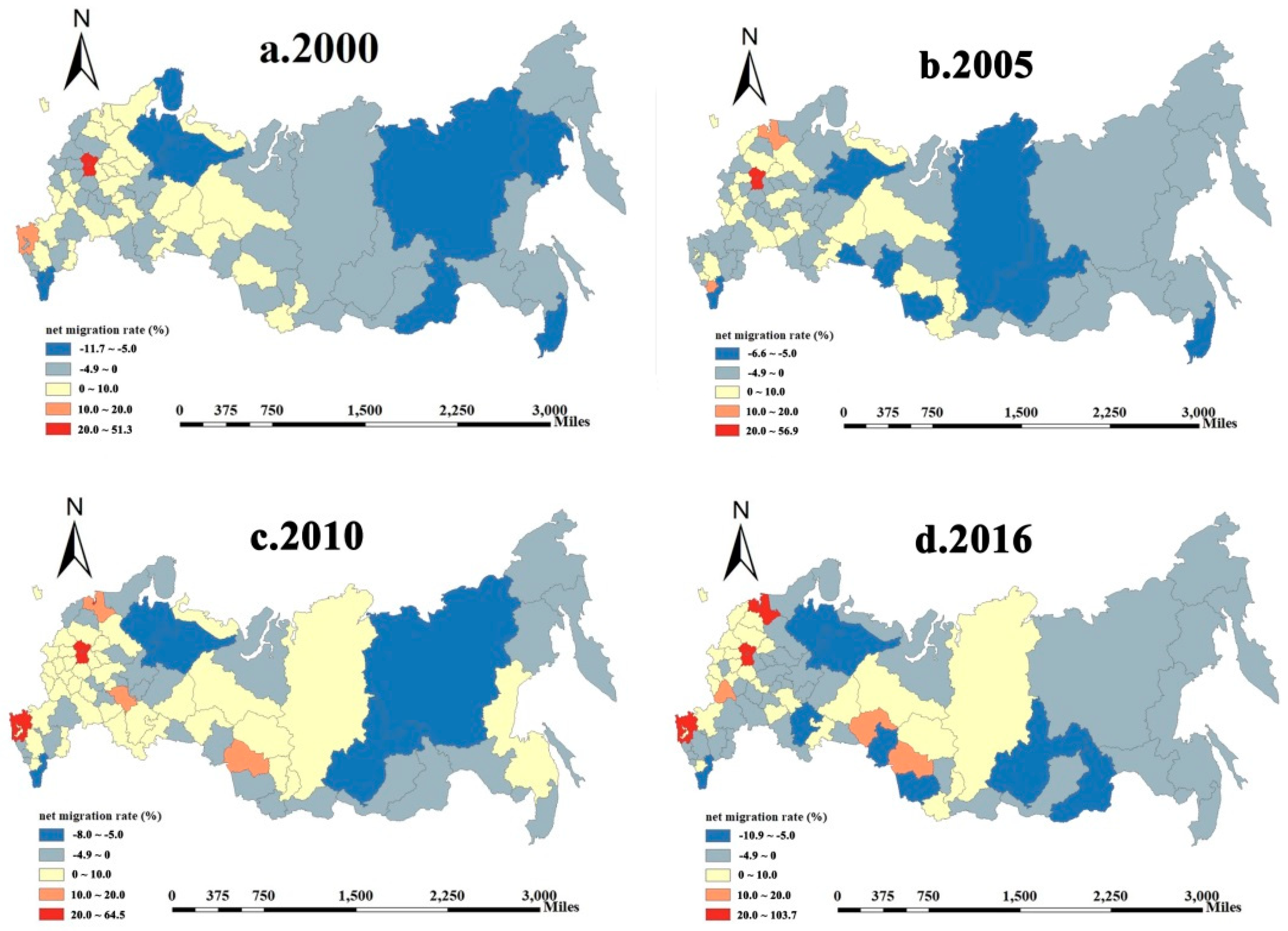
At the national level, the net migration rate is 1.7 per 1000 population in 2017. At regional level, the migration pattern experienced slight change in the past 4 periods and the influx area is mainly in the west European region, while the out flux area is the East and some regions in the North like Komi Republic. In 2016, Daghestn Republic has experienced the largest population loss while Moscow oblast has the largest population gain with the net migration rate being -10.91 and 103.4 per 1000 population, respectively (see Figure 1).

Although with a slight increase between 2008–2010, the unemployment in Russia in general experienced a downward trend with the rate being 5.17 percent in 2018. The regional unemployment pattern is similar with the national trend, with the lowest unemployment rate of 1.3 in Moscow City and 26.8 in Ingush Oblast (S1a). The per capita GRP sees a significant improvement in the past 15 years, averagely from 1171USD in 2000 to 10743USD in 2017. At regional level, the economic level varies significantly with per capita GRP ranging from 5085USD in Ingush Oblast to 227793USD in Nenet Oblast (S1b). Life expectancy represents the general health related wellbeing of the society [40] and infant mortality is one of the child health care system indicators [41]. In Russia, the average life expectancy increase from 65.48 in 2000 to 71.59 in 2016. Regionally, the Ingush Oblast has the highest life expectancy of 80.82 years, followed by Dagestan and Moscow City and the Tuva Republic has the lowest life expectancy of 64.21 years (S1c). The infant mortality sees a significant decrease from the average of 16.6 in 2000 to 7.6 per 1000 in 2016. Chukot Republic has the highest infant mortality rate of 16.1, while Magada and Nenets have the lowest infant mortality rate of 2.1 (S1d). The urbanization rate in Russia fluctuates in the past 15 years with very tiny increase to 74.2 in 2016. Urban scale also sees a slight increase, with the smallest of 11sqm in Chukot Republic and the largest of 2480 sqm in Moscow Oblast in 2016(S1e, S1f).

4.2. The Correlation Between Migration and Socioeconomic Factors in Russia

The Pearson correlation indicates that apart from per capita GRP, all of the rest variables included show significant correlations with the net migration (

Table 1. Pearson correlation between net migration and variables at each time period.

Pearson Correlation	2000	2005	2010	2015/2016
Unemployment rate	−0.402 **	−0.110	−0.266 *	−0.252 *
per capita GRP	0.144	0.054	0.072	0.177
Urbanization rate	0.301 **	0.261 *	0.309 **	0.193
Urban scale	0.351 **	0.400 **	0.561 **	0.529 **
Life expectancy	0.061	0.281 *	0.275 *	0.237 *
infant mortality	−0.324 **	−0.111	−0.267 *	−0.208

*. Significant correlation at 0.05 level (2-tail); **. Significant correlation at 0.01 level (2-tail); N = 82.

). Low unemployment rate and higher urbanization are all attracting factors for population influx. Higher life expectancy and lower infant mortality rate are all positively related to the population influx.

4.3. The Spatial Aggregation of Net Migration Rate

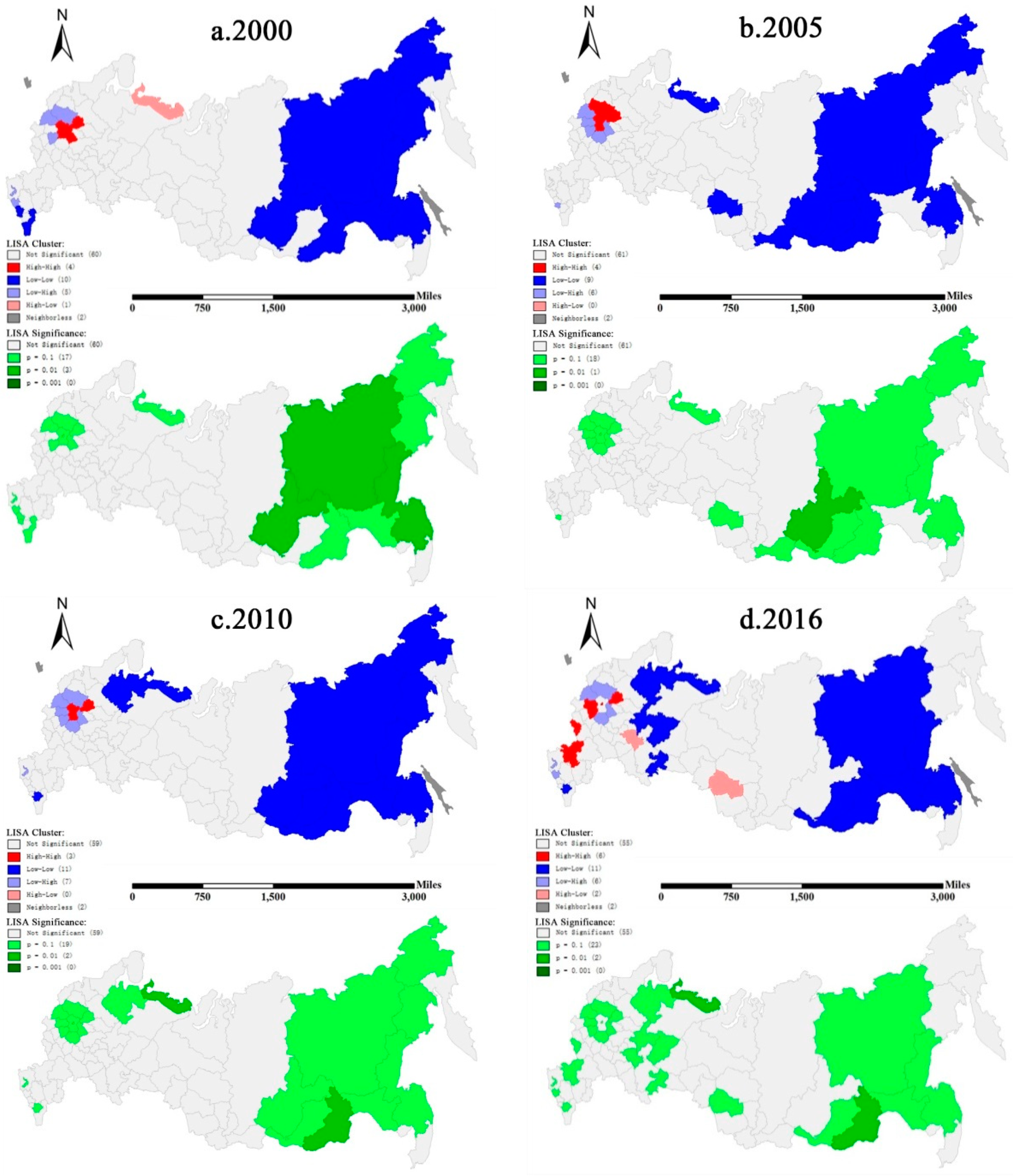
The global Moran’s I indicates there is spatial correlation within the net migration (

Table 2. Moran’s I of net migration in Russia.

	2000	2005	2010	2016
Moran’s I	0.145431	0.182935	0.191498	0.099421
Z-value	2.768039	3.340151	3.298386	1.922572
p-value	0.005639	0.000837	0.000972	0.054534

Moran’s I is between -1~1; The threshold for Z value is 1.65, if Z-value is above 1.65 and P is lower than 0.05 or 0.01, indicating the chance that dataset is spatially clustered are high.

) and through the local indicators of spatial association (LISA) analysis, the clusters of the spatial associations are identified in Figure 2.

In general, the “low-low” migration are located in the Far East region, while the “high-high” and “low-high” are located in the surrounding of the Moscow city. The Nenets okray experienced a “high-low” cluster in 2000 and “low-low” pattern since then. The net migration in 2016 experienced an obvious diverse cluster pattern comparing with the former periods. Regions in the west European region (including Rostove oblast, Belgorod oblast and Volgograd oblast) has more “high-high” migration pattern, indicating the region has become more attractive in terms of migration.

4.4. Spatial Panel Econometric Analysis on the Driving Forces for Russia Migration

In order to identify the best-fit model to explore the driving factors and driving patterns on net migration, we conducted a series of test. First, simple OLS technique was run on Panel data, with spatial fixed, time-period fixed and spatial and time period fixed estimations (

Table 3. Panel data model estimation results without spatial interaction.

	OLS	Spatial Fixed Effects	Time-Period Fixed Effects	spatial and Time-Period Fixed Effects
R2	0.4773	0.2840	0.3148	0.2249
σ2	65.8341	18.9210	84.5581	19.0463
LMlag	9.2966 ***	0.0084	9.0771 ***	0.0009
R_LMlag	0.5836	0.0009	0.2041	0.0977
LMerror	13.9802 ***	0.0075	9.9281 ***	0.0281
R_LMerror	5.2672 **	0.0001	1.0551	0.1249

Note: ***, **, * respectively indicate the significant test at the confidence level of 1%, 5% and 10%.

).

Both LMlag and LMerror from OLS and time-period fixed model significantly rejected the null hypothesis of “there is no spatial effect of the variables on the net migration,” indicating the model has to include the spatial effect of the variables. However, both R_LMlag and R_LMerror from the four models (except for R_LMerror in OLS) did not pass the significant test, allows to accept the hypothesis. Thus, it is necessary to conduct Wald test and LR test in SDM model and see whether the SDM model can be simplified to the SAR or SEM (see

Table 4. Panel data model LR test results.

	LR Value	Degrees of Freedom	p-Value
LR-test joint significance spatial fixed effects	488.9055	82	<0.001
LR-test joint significance time-period fixed effects	4.5657	4	0.0335

).

Through the LR test, the P-values from both spatial fixed effects and the time-period fixed effects are significant (at 1% and 5% level), rejected the null hypothesis of no spatial fixed effect and no time-period effect. The next step is thus to include both time effect and spatial effect in the spatial panel model (see

Table 5. SDM model Wald test and LR test results.

	Spatial Fixed Effects	Time-Period Fixed Effects	Spatial and Time-Period Fixed Effects
Wald spatial lag	10.0961	10.9366 *	8.5809
Wald spatial error	9.9324	19.6904 ***	8.5879
LR spatial lag	9.9352	11.1009 *	8.4647
LR spatial error	22.2957 ***	10.6829 *	8.4385

Note: ***, **, * respectively indicate the significant test at the confidence level of 1%, 5% and 10%.

).

In spatial fixed effect model, LR test indicated that SDM rejected to be simplified to SEM (LR spatial error = 22.2957 ***). In time-period fixed effect model, SDM significantly rejected to be simplified to SEM and rejected to be simplified to SLM at 10% level. In spatial and time-period fixed effects analysis, SDM accepted to be simplified to SEM and SLM. Thus, spatial fixed effects SLM, time-period fixed effects SLM, time-period fixed effects SDM and spatial and time-period fixed effects SDM have to be conducted to identify the best fit model.

Based on the LM and R_LM test results, the significances of the explanatory variables, the Corrected R2 value and the Log-Likelihood in

Table 6. Estimation results of panel model with different specific effects.

	Spatial Fixed Effects SLM	Time–Period Fixed Effects SLM	Time–Period Fixed Effects SDM	Spatial and Time–Period Fixed Effects SDM
per capita GRP	0.000125 ***	0.000049 *	0.000047 *	0.000126 ***
Unemployment_Rate	0.209779 **	−0.325412 **	−0.347043 ***	0.092462
Life_expectancy_years	0.157998	1.066974 ***	1.03087 ***	0.281871
urbanization_rate	0.114774 ***	0.053446	0.031569	0.187175
urban scale	256.298046 ***	118.63219 ***	118.812804 ***	265.389294 ***
infant_mortality_ratio < 1	0.276749	0.222855	0.195117	0.153577
W* per capita GRP			0.000098	0.000079
W*Unemployment_Rate			0.003317 **	0.130637
W*Life_expectancy_years			0.143679	0.480591
W*urbanization_rate			−0.035624	0.193501
W* scale			−52.899037 *	−123.141725 *
W*infant_mortality_ratio < 1			−0.173621	0.412575 **
W*dep.var.	−0.00698	0.20998 ***	0.23498 ***	−0.012992
σ2	18.9594	79.8663	77.0925	18.2219
R2	0.8457	0.3501	0.3726	0.8517
Corrected R2	0.2668	0.3109	0.3302	0.2446
Log–Likelihood	−947.95029	−1185.5809	−1180.0305	−941.43865

Note: ***, **, * respectively indicate the significant test at the confidence level of 1%, 5% and 10%.

, the time-period fixed effects SDM was chosen as the best fit model.

Table 7. Direct and indirect effects of different factors on net migration in Russia.

	Coefficient	Direct	Indirect	Total
Per capita GRP	0.000047 *	0.000054 **	0.00013 5 **	0.000189 ***
Unemployment_Rate	−0.347043 ***	−0.351979 ***	−0.096041	−0.448020
Life_expectancy_years	1.03087 ***	1.052211 ***	0.487821 ***	1.540032 ***
urbanization_rate	0.031569	0.029438	−0.036724	−0.007286
urban scale	118.812804 ***	117.548070 ***	−28.734603	88.813467 **
infant_mortality_ratio < 1	0.195117	0.184359	−0.174434	0.009925
W* Per capita GRP	0.000098 **
W*Unemployment_Rate	0.003317
W*Life_expectancy_years	0.143679
W*urbanization_rate	−0.035624	Hausman test
W*urban scale	−52.899037 *	66.0979 ***
W*infant_mortality_ratio < 1	−0.173621	W*dep.var z-probability
W*dep.var.	0.23498 ***	0.000808

Note: ***, **, * respectively indicate the significant test at the confidence level of 1%, 5% and 10%.

shows the direct and indirect effects of different variables on net migration in Russia. The W*dep.var. being significant at 1% level exerts a positive spillover effect on the net migration. Hausman test significantly rejects the random effect model and favor fixed effect model. The estimation result shows that variable per capita GRP, life expectancy and urban scale have positive and significant (at 10%, 1% and 1% level) effect in the model, while unemployment has significant negative effect in the model (coefficient is significant at 1% level). This means, a better per capita GRP, health related wellbeing and larger urban scale would have favored the net migration; regional per capita GRP and wellbeing have a positive effect on the net migration, while unemployment shows the contrary result. Per capita GRP and life expectancy also show positive spillover effect, which means, the increase of per capita GRP and better life expectancy in neighboring regions increase the net migration in such a region and the increase of per capita GRP and life expectancy in a region increase the net migration in nearby regions. Unemployment shows no spillover effect on net migration, indicating the increase of the employment rate will potentially increase the net migration in its own region but not the neighboring regions.

The effects in Table 7 also indicate the extent to which the variable can influence the net migration. Every 100 USD increase in per capita GRP would lead to averagely 5.4 net migrates in the region; every 1 year increase in life expectancy would increase 1052 net migrates; every 1sqm increase in urban area would increase the net migrates by 11.75, while for unemployment, every 1% increase in unemployment would lead to decrease of 0.54 net migrates. The influence of the neighboring variables has much smaller effect on the net migration in the region in general.

Per capita GRP and life expectancy has obvious spillover effect (indirect effect in Table 7). Averagely 1 year increase in life expectancy in the neighborhood would increase 487 net migrates. For per capita GRP, the spillover effect is even stronger than direct effect, with every 100 USD increase in the neighborhood per capita GRP leading to averagely 13.5 net migrates in the region.

5. Discussion and Policy Implications for Russia Far North and East

This study quantifies the impact of socioeconomic factors on migration using spatial panel econometric analysis and the spillover effect is also found in the analysis. Among the factors included, per capita GRP and life expectancy have significant influence on migration, both directly and indirectly, while unemployment rate and urban scale have significant direct influence on migration. It is obvious that regions with higher economic status and larger urban scale attract people, which is similar with former researches [13,26], where higher income attract people, while higher unemployment demotivates them. The densely populated regions, where always accompanied with larger urban scale, have cumulative effect for inward migration and the intensive reduction of the population size results in the decline of the demographic and labor potential of the area [31,42]. Our study also supports this theory.

The added value of the present study is that health-related wellbeing can contribute to migration. Vakulenko showed that the government expenditure on health care is one of the most important budget spending areas for migration [26], which is in accordance with the current result. Another innovative value is the “spillover effect,” meaning that the neighborhood’s socioeconomic status can also influence the attractiveness of one region.

Based on the economic driven migration theory, Vakulenko suggested to creating economic zones to stimulate migration activity [26]. Whereas, according to Reisser [36], in the Far North, the socioeconomic vitality varies significantly among places, largely driven by the energy industries and this pattern is somehow shaping a population polarization. Combining our “spillover effect,” we propose that merely an economic zone is not enough to pull the whole area together out of the losing-population phenomenon. A specific functional zoning plan considering the economic, natural resource, geographic location characteristics of each region is suggested. First and foremost is the resource zone. Russia Far North and Far East have abundant natural resources and the central government is putting much emphasis on developing these regions. The Russia Arctic region has the highest amount of petroleum comparing with the other Arctic regions at national level, accounting for over than 37% of the total petroleum in the Arctic region. The revenue of the oil and gas accounts for over than 22% of the total Russia economic in 2013 and this number is still increasing [43]. Utilizing the natural resources in the Far North region (some regions) is the primary and the one of major goals of Russia’s Arctic development strategy [34]. Far East development is set as the national priority, particularly focus on Sino-Russia collaboration in this region. Recently, the Russia and China government issued a “The Plan on China-Russia Cooperation and Development in the Russian Far East Region (2018-2024)” to boost the economic growth in the Far East region with a series of concrete economic incentives [44]. The second is the traffic zone, the Far North and Far East have very specific geo-locations. The Far East region has the predominant geo-location connecting Asia-Pacific market, while the Arctic region covers almost all the key ports for Arctic Northeast Route. Both are extreme important for resources circulations. Apart from these, some other resources mainly including ecological resources and tourism resources can also play some role in the regional zoning. These resources are not evenly geographically distributed; therefore, a strategic plan should be made to promote a balanced and complementary socioeconomic growth in the area instead of a polarization development.

Former research has indicated that there might be a turning point for the amount of labor because of high salary from exploitation of natural resources [8]. The climate change is amplifying in the High North. Together with the increasingly emphasis on the Arctic development and the opening up of Arctic shipping routes from Russia government, accompanied with strong push from China to facilitate the “Ice silk road,” a prosperity of Russia Arctic region can be speculated in the near future. But, one should keep in mind that merely economic or job opportunities (employment) cannot make a region prosperous and attractive in a long way and the result from current study support the fact that the health related wellbeing and urban development also plans key role in terms of net migration.

In addition, it is needed to refer that the economic and socio-cultural life can also be altered by the migration, as the urban expansion is likely accompanied with social problems like crime and the sparse-populated regions are particularly vulnerable in terms of population in/out-flux. For example, majority of external migration are skilled migration, the influx of those people for one hand, contribute to the economic, on the other hand, leading to culture contradictions and increased the competitiveness of job market [1]. In this context, gaining the support from the local residence and community is of vital importance. Enhancing the trust of the local residence to the government could facilitate the infrastructure build-up and enhance the social exchange and social integration. This can be achieved through the perceived power and benefits of the local residence, not only the economic or social benefits but also the benevolence, ability and integrity of the influx population [45,46].

6. Conclusions

Using spatial panel econometric analysis, the influence of socioeconomic variables on the net migration in Russia was studied and four conclusions can be summarized. First, economic development, represented by employment rate and per capita GRP have positive effect for net migration; Second, urban development, particularly the size of urban area, has pulling effect for the immigrates; Third, a better health related wellbeing also has positive effect for immigration; And fourth, a better situation of economic and health related wellbeing can not only increase the attractiveness for one region but also for the neighborhood regions.

Limitations of the study are also evident and should be bridged in the future study. First, the model rejects the lag effect and this is most likely because of the non-time series data. Five-year time span might be too large for lag effect. Second, the data we used are total migration, so we could not get a clear picture on why people migrate or immigrate and the reason behind might be different. Third, the variables we included covering only some of the factors that might influence the migration, we believe the result would be more interesting if more variables are included.

References

- Laruelle, M. The demographic challenges of Russia’s Arctic. Russ. Anal. Dig. 2011, 9, 8–12. [Google Scholar]
- Kekkonen, A.; Shabaeva, S.; Gurtov, V. (Eds.) Human capital development in the Russian Arctic. In Interconnected Arctic-UArctic Congress 2016; Springer Polar Sciences; Springer: Cham, Switzerland, 2016. [Google Scholar] [CrossRef]
- Ioffe, G.; Zayonchkovskaya, Z. Immigration to Russia: Inevitability and prospective inflows. Eurasian Geogr. Econ. 2010, 51, 104–125. [Google Scholar] [CrossRef]
- Anisimova, T.V.; Konfisakhor, A.G.; Samuylova, I.A.; Konfisakhor, A.G.; Anisimova, T.V. Migration as an indicator of people’s social and psychological stability (as exemplified in the Pskov Region). Psychol. Russ. State Art 2015, 8, 61. [Google Scholar]
- Kumo, K. Inter-regional population migration in Russia: Using an origin-to-destination matrix. Post-Communist Econ. 2007, 19, 131–152. [Google Scholar] [CrossRef]
- Kashnitskiy, I.; Mkrtchyan, N.; Leshukov, O. Interregional migration of youths in Russia: A comprehensive analysis of demographic Statistics. Voprosy Obrazovaniya/Educ. Stud. 2016, 3, 169–203. [Google Scholar] [CrossRef]
- Sokolova, F. Migration processes in the Russian Arctic. Arct. North 2016, 25, 158–172. [Google Scholar] [CrossRef]
- Sardadvar, S.; Vakulenko, E. A model of interregional migration under the presence of natural resources: Theory and evidence from Russia. Ann. Reg. Sci. 2017, 59, 535–569. [Google Scholar] [CrossRef]
- Gerber, T.P. Regional Migration Dynamics in Russia since the Collapse of Communism; University of Arizona: Tucson, AZ, USA, 2000. [Google Scholar]
- Vakulenko, E.S. Does Migration Lead to Regional Convergence in Russia? IJEPEE. 2016, 9, 1–25. [Google Scholar] [CrossRef]
- Etzo, I. The determinants of the recent interregional migration flows in Italy: A panel data analysis. J. Reg. Sci. 2011, 51, 948–966. [Google Scholar] [CrossRef]
- Mkrtchyan, N.V. Migration mobility in Russia: Evaluation and problems. SPERO 2009, 11, 149–164. [Google Scholar]
- Kumo, K. Interregional migration: Analysis of origin-to-destination matrix. In Demography of Russia, Studies in Economic Transition; Palgrave Macmillan: London, UK, 2016; pp. 261–314. [Google Scholar]
- Dmitrieva, O. Regional Development: The USSR and after; Palgrave Macmillan: London, UK, 1996. [Google Scholar]
- Rafael, R. Climate change-induced migration and violent conflict. Political Geogr. 2007, 26, 656–673. [Google Scholar]
- Shestakov, A.; Streletsky, V. Mapping of Risk Areas of Environmentally-Induced Migration in the Commonwealth of Independent States; International Organization for Migration: Geneva, Switzerland, 1998. [Google Scholar]
- Kane, H. The Hour of Departure: Forces that Create Refugees and Migrants; Paper 125; Worldwatch: Washington, DC, USA, 1995. [Google Scholar]
- Grigoriev, A.; Ushakov, D.; Valueva, E.; Zirenko, M.; Lynnc, R. Differences in educational attainment, socio-economic variables and geographical location across 79 provinces of the Russian Federation. Intelligence 2016, 58, 14–17. [Google Scholar] [CrossRef]
- Demidova, O.; Marelli, E.; Signorelli, M. Spatial effects on youth unemployment rate: The case of Eastern and Western Russian regions. East. Eur. Econ. 2013, 51, 94–124. [Google Scholar] [CrossRef]
- Yormirzoev, M. Determinants of labor migration flows to Russia: Evidence from Tajikistan. Econ. Sociol. 2017, 10, 72–80. [Google Scholar] [CrossRef]
- Tartakovsky, E.; Patrakov, E.; Nikulina, M. Factors affecting emigration intentions in the diaspora population: The case of Russian Jews. Int. J. Intercult. Relat. 2017, 59, 53–67. [Google Scholar] [CrossRef]
- Andrienko, Y.; Guriev, S. Determinants of Interregional Mobility in Russia: Evidence from Panel Data. William Davidson Working Paper Number 551. 2003. Available online: https://deepblue.lib.umich.edu/bitstream/handle/2027.42/39936/wp551.pdf?sequence=3 (accessed on 20 February 2019).
- O’Loughlin, J.; Panin, A.; Witmer, F. Population change and migration in Stavropol’ Kray: The effects of regional conflicts and economic restructuring. Eurasian Geogr. Econ. 2007, 48, 249–267. [Google Scholar] [CrossRef]
- Vakulenko, E.; Mkrtchyan, N.; Furmanov, K. Econometric analysis of internal migration in Russia (Ekonometrijska Analiza Unutrasnjih Migracija U Rusiji). Montenegrin J. Econ. 2011, 7, 21–33. [Google Scholar]
- Guriev, S.; Vakulenko, E. Breaking out of poverty traps: Internal migration and interregional convergence in Russia. J. Comp. Econ. 2015, 43, 633–649. [Google Scholar] [CrossRef] [Green Version]
- Vakulenko, E.S. Econometric analysis of factors of internal migration in Russia. Reg. Res. Russ. 2016, 6, 344–356. [Google Scholar] [CrossRef]
- Mkrtchyan, N.V.; Florinskaya, Y.F. Labor migration in Russia: International and internal aspects. Zhurnal Novaya Ekon. Assotsiatsiya-J. New Econ. Assoc. 2018, 1, 186–193. [Google Scholar] [CrossRef]
- Gerber, T.P. Individual and Contextual Determinants of Internal Migration in Russia: 1985–2001; University of Wisconsin: Madison, WI, USA, 2005. [Google Scholar]
- Karachurina, L.B. Demographic transformation of post-Soviet cities of Russia. Reg. Res. Russ. 2014, 4, 56–67. [Google Scholar] [CrossRef]
- Sardadvar, S.; Vakulenko, E. Interregional migration within Russia and its east-west divide: Evidence from spatial panel regressions. Rev. Urban Reg. Dev. Stud. 2016, 28, 123–141. [Google Scholar] [CrossRef]
- Makhrova, A.G.; Nefedova, T.G.; Pallot, J. The specifics and spatial structure of circular migration in Russia. Eurasian Geogr. Econ. 2016, 57, 802–818. [Google Scholar] [CrossRef]
- Efremova, I.; Didenko, N.; Rudenko, D.; Skripnuk, D.F. Disparities in rural development of the Russian arctic zone regions. Economics 2017, 2, 189–194. [Google Scholar]
- Metelev, S.E. Labor migration in Russia as the reflection of macroeconomic trends. Life Sci. J. 2014, 10, 709–712. [Google Scholar]
- Russia’s Arctic Policy to 2020 and Beyond. Adopted by the President of the Russian Federation. 2009. Available online: http://www.arctis-search.com/Russian+Federation+Policy+for+the+Arctic+to+2020 (accessed on 20 February 2019).
- Vitalyevna, T.; Nikolaevich, A. Law on strategic planning in the Russian Federation: Advantages and unresolved issues. Econ. Soc. Chang. 2014, 4, 63–67. [Google Scholar]
- Reisser, C. Russia’s Arctic Cities: Recent Evolution and Drivers of Change. In Sustaining Russia’s Arctic Cities: Resources Politics, Migration and Climate Change; Orttung, R., Ed.; Berghahn: New York, NY, USA, 2017; Chapter 1. [Google Scholar]
- Wong, D.; Lee, J. Statistical Analysis of Geographic Information with ArcView GIS and ArcGIS; Wiley: New York, NY, USA, 2005. [Google Scholar]
- Anselin, L. Spatial Econometric: Methods and Models. J. Am. Stat. Assoc. 1990, 85, 160. [Google Scholar]
- Lesage, J.; Pace, R.K. Introduction to Spatial Econometrics; CRC Press: New York, NY, USA, 2009. [Google Scholar]
- OECD. OECD Better Life Index. 2019. Available online: http://www.oecdbetterlifeindex.org/topics/health/ (accessed on 5 March 2019).
- Baranov, A.; Namazova-Baranova, L.; Albitskiy, V.; Ustinova, N.; Terletskaya, R.; Komarova, O. The Russia child health care system. J. Pediatr. 2016, 177S, 148–155. [Google Scholar] [CrossRef]
- Lutsenko, E.; Bazhenova, N.; Bogachenko, N.; Averina, O.; Nikolaeva, P.; Korolyova, I. Migration processes among the youth of the Far Eastern region of the Russian Federation. Eurasian J. Anal. Chem. 2017, 12, 1429–1434. [Google Scholar] [CrossRef]
- Rosstat. Russian Federation Federal State Statistics Service. 2018. Available online: http://www.gks.ru/wps/wcm/connect/rosstat_main/rosstat/en/main/ (accessed on 10 February 2019).
- Ministry of Commerce PRC. The Plan on China-Russia Cooperation and Development in the Russian Far East Region (2018–2024). 2018. Available online: http://english.mofcom.gov.cn/article/newsrelease/policyreleasing/201811/20181102808296.shtml (accessed on 1 February 2019).
- Nunkoo, R.; Ramkissoon, H. Developing a community support model for tourism. Ann. Tour. Res. 2011, 38, 964–988. [Google Scholar] [CrossRef]
- Nunkoo, R.; Ramkissoon, H. Power, trust, social exchange and community support. Ann. Tour. Res. 2012, 39, 997–1023. [Google Scholar] [CrossRef]
Figure 1.
Net migration rate in the four periods.
Figure 2.
LISA for the net migration in the four periods, (a) for 2000, (b) for 2005, (c) for 2010 and (d) for 2016.