Analysis and Prediction of Water Quality Using LSTM Deep Neural Networks in IoT Environment

Abstract

This research paper focuses on a water quality prediction model which requires high-quality data. In the process of construction and operation of smart water quality monitoring systems based on Internet of Things (IoT), more and more big data are produced at a high speed, which has made water quality data complicated. Taking advantage of the good performance of long short-term memory (LSTM) deep neural networks in time-series prediction, a drinking-water quality model was designed and established to predict water quality big data with the help of the advanced deep learning (DL) theory in this paper. The drinking-water quality data measured by the automatic water quality monitoring station of Guazhou Water Source of the Yangtze River in Yangzhou were utilized to analyze the water quality parameters in detail, and the prediction model was trained and tested with monitoring data from January 2016 to June 2018. The results of the study indicate that the predicted values of the model and the actual values were in good agreement and accurately revealed the future developing trend of water quality, showing the feasibility and effectiveness of using LSTM deep neural networks to predict the quality of drinking water.

1. Introduction

With the rapid development of economy and accelerated urbanization, water pollution has become more and more serious [1]. Therefore, understanding the problems and trends of water pollution is of great significance for the prevention and control of water pollution. In order to fully understand the quality of the water environment, most cities in China have started the construction of water environment monitoring systems. The development of remote sensing (RS) [2,3], Internet of Things (IoT) [4,5,6,7,8], cloud computing, big data and artificial intelligence (AI) provides new opportunities and approaches for the innovation and application of water environment monitoring technology. Relying on different kinds of hydrological and water quality automatic monitoring stations, RS monitoring systems, wireless sensor networks (WSNs), monitoring ships, and advanced underwater bionic robots, smart monitoring systems for water environment protection have been built in cities and counties in China.

On the basis of the historical data collected by the smart water quality monitoring systems, a water quality prediction model can establish a corresponding mapping relationship between the multi-monitoring data and the changes of water quality parameters and can predict changes of water quality status in certain future periods. In recent years, the establishment of reliable water quality prediction models [9,10,11,12,13,14,15,16] has become one of the research hotspots in the field of water environmental science. However, with the large-scale application of the smart water quality monitoring systems, although the shortcomings of the traditional collection method are solved, a large amount of big data is produced. In addition, the water environment is affected by many factors and has strong nonlinear characteristics. However, the traditional water quality prediction model cannot comprehensively consider the influence of physics, chemistry, biology, meteorology, and hydraulics factors. At present, researchers mainly focus on improving the applicability and reliability of water quality prediction models and have introduced a variety of new technologies, such as fuzzy mathematics, stochastic mathematics, 3S technology, artificial neural networks (ANN), etc., to improve water quality prediction models and promote the scope of applications [17,18].

Among the technologies mentioned above, ANN has become a popular method for water quality prediction because of its excellent applicability to uncertain and nonlinear situations. As a typical representative of artificial neural networks, the traditional back-propagation (BP) neural network and its improved algorithms have obvious advantages in predicting nonlinear problems and have been effectively applied to water quality prediction [19]. The radial-basis-function (RBF) neural network has been widely used in prediction research in various water environment by virtue of its simple structure, fast training speed, and ability to approximate arbitrary functions globally with arbitrary precision [20,21]. However, the above artificial neural network models are not suitable for time-series prediction problems. The so-called time series is a series of observations in chronological order. The automatic water quality monitoring station of drinking water source automatically collects water quality parameters at a fixed time interval (such as on a daily basis) and uploads them to a server to reflect the fluctuations of water quality at regular intervals at the monitoring points. Therefore, water quality parameters appear in the form of time series. Due to the good performance of long short-term memory (LSTM) models in time-series prediction, the application of LSTM in environmental research has become more and more extensive [22]. However, few studies have applied the LSTM models to the prediction of drinking-water quality parameters.

This paper proposes a drinking-water quality prediction model based on LSTM deep neural networks to predict drinking-water quality data measured by the automatic water quality monitoring station of the Guazhou Water Source in Yangzhou City and then compares the predicted results with the measured data. The results show the potential of application of LSTM and deep learning in predicting drinking water quality.

2. Data Source and Pre-Processing

2.1. Study Area Description and Water Quality Data Analyzed

With the popularization and application of IoT, water quality monitoring has gradually evolved into automation and networking. Yangzhou City, Jiangsu Province, China, as the source city of the East Route of the South-to-North Water Diversion Project, has organized the water quality monitoring of major rivers (lakes) for many years and established a water quality monitoring and control system at the city and county levels, with drinking-water source protection as the main objective. The main urban area of Yangzhou includes users within towns and townships where regional water supply has been implemented. There are three main water sources: one in the waters of Liaojiagou, the river embayment of the Huaihe River, one in the Guazhou section of the Yangtze River, and the one in Sanjiangying of Yangtze River in Touqiao town. The three water intakes are abundant in water, and the water quality is stable and meets the national second-class drinking-water source water quality standards. In order to protect the water sources, Yangzhou Environmental Protection Bureau has carried out real-time monitoring to the water intakes. Up to now, a number of automatic water quality monitoring stations have been built in the water source areas of Sanjiangying, Guazhou, Liaojiagou, Wanfu Gate, and Shierwei downstream of the Yangzhou Chemical Industry Park to ensure continuous monitoring of water quality status all day long. On the basis of actual needs, the commonly used six water quality parameters are collected and uploaded to the monitoring center server of Yangzhou Environmental Protection Bureau to form an automatic water quality monitoring network covering urban drinking-water sources.

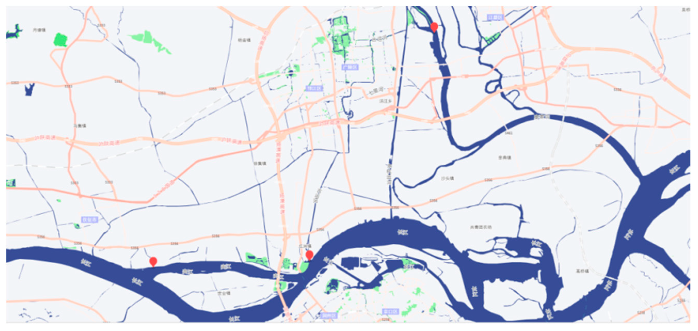
Figure 1 is a location map of some water quality automatic monitoring stations in Yangzhou water source area extracted by using the Gaode map API/SDK interface. The three red balloons shown in the figure are the locations of water quality automatic monitoring stations in Shierwei, Guazhou, and Wanfu Gate, from the left to the right. The blue area is part of the water system of the Yangzhou section of the Yangtze River.

The experimental data samples in this paper were collected from the water quality monitoring data from 1 January 2016 to 30 June 2018 in the automatic water quality monitoring station of Guazhou Water Source, Yangzhou City of Yangtze River, with a total of 912 groups. The water source of Guazhou belongs to the Yangtze River system and is a river-type water source. The Guazhou water quality automatic monitoring station automatically collects six water quality parameters and water temperatures at a fixed time every day and uploads them to the server.

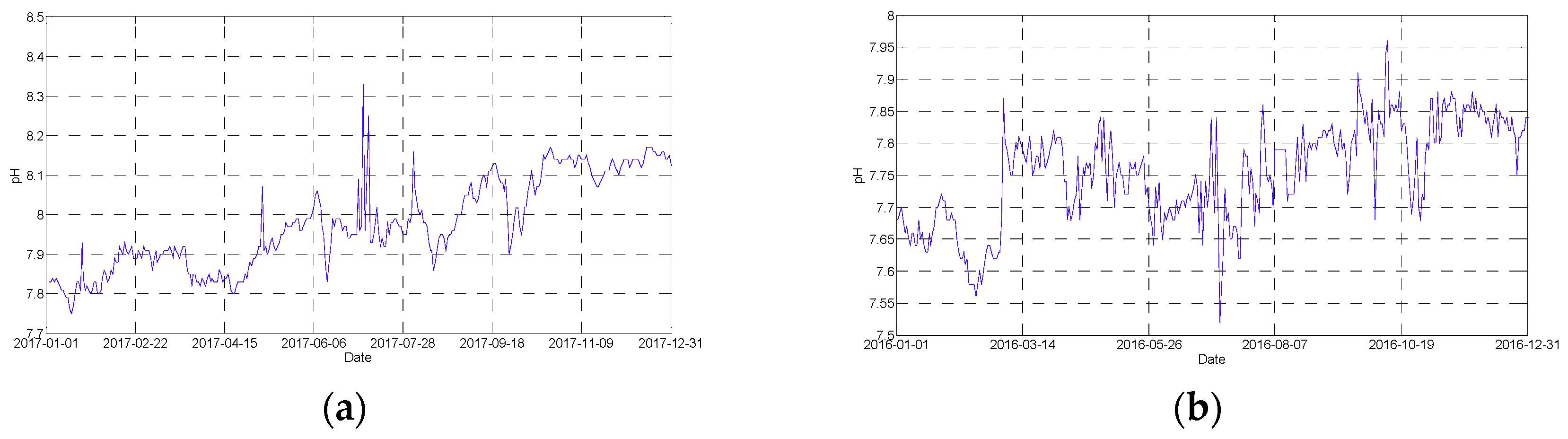
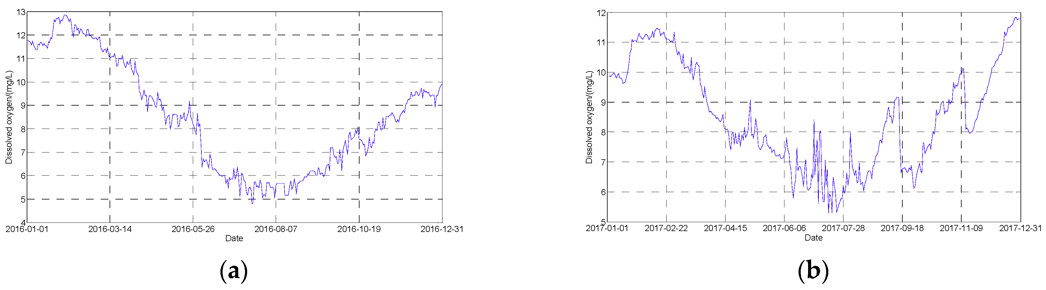
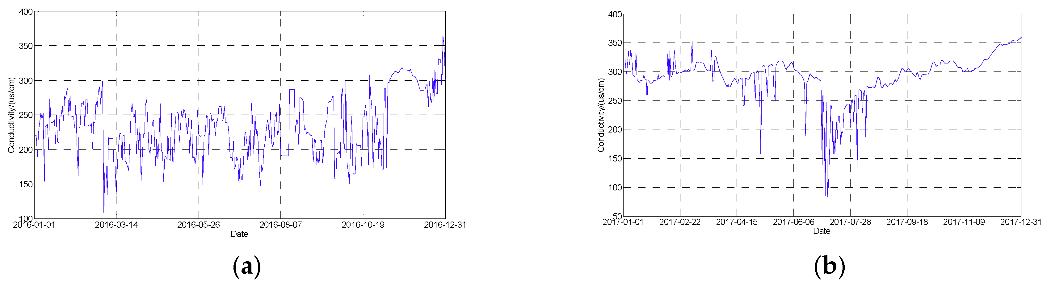
According to the 731 sets of water quality monitoring data collected in 2016 and 2017, the time variation trend of water quality parameters of the water source of the Yangtze River in Guazhou was analyzed. For time-series data, we drew a line graph to reflect the characteristics of each water quality parameter over time. Figure 2, Figure 3, Figure 4, Figure 5, Figure 6 and Figure 7 show the annual trends of pH, dissolved oxygen, conductivity, turbidity, chemical oxygen demand (CODMn), and NH₃–N in 2016 and 2017.

Table 1. Monthly mean values of water quality monitoring parameters of Guazhou Water Source in 2016.

Month	Water Temperature/(°C)	pH	Dissolved Oxygen/(mg/L)	Conductivity/(us/cm)	Turbidity/(NTU)	CODMn/(mg/L)	NH3-N/(mg/L)
January	9.7	7.67	11.90	238	81	3.12	0.30
February	9.3	7.62	12.26	248	55	2.50	0.13
March	12.7	7.78	11.14	203	64	2.26	0.13
April	17.2	7.76	9.52	209	84	2.61	0.13
May	21.0	7.74	8.39	222	75	1.68	0.13
June	24.4	7.71	6.23	224	76	1.81	0.19
July	26.6	7.71	5.54	207	136	3.19	0.17
August	30.0	7.77	5.58	241	105	2.61	0.16
September	26.9	7.81	6.35	220	101	2.53	0.17
October	22.1	7.80	7.36	217	97	3.01	0.14
November	16.9	7.84	8.47	288	110	2.58	0.16
December	12.9	7.83	9.51	298	119	2.55	0.24

and

Table 2. Monthly mean values of water quality monitoring parameters of Guazhou Water Source in 2017.

Month	Water Temperature/(°C)	pH	Dissolved Oxygen/(mg/L)	Conductivity/(us/cm)	Turbidity/(NTU)	CODMn/(mg/L)	NH3-N/(mg/L)
January	10.4	7.81	10.36	294	95	2.54	0.30
February	10.0	7.89	11.21	300	68	1.89	0.35
March	12.7	7.88	9.91	309	100	2.26	0.19
April	16.9	7.84	8.08	281	115	2.55	0.08
May	21.8	7.95	7.71	297	83	1.57	0.08
June	24.8	7.97	6.79	286	105	1.88	0.18
July	27.6	7.99	6.23	208	123	2.65	0.21
August	29.7	7.97	6.92	264	95	1.87	0.19
September	27.4	8.06	7.58	294	105	1.67	0.20
October	22.8	8.10	8.20	311	133	1.99	0.20
November	18.9	8.12	8.97	308	97	1.77	0.14
December	13.7	8.14	11.03	348	98	1.87	0.17

show the monthly average values of water quality monitoring parameters of the water source in Guazhou in 2016 and 2017.

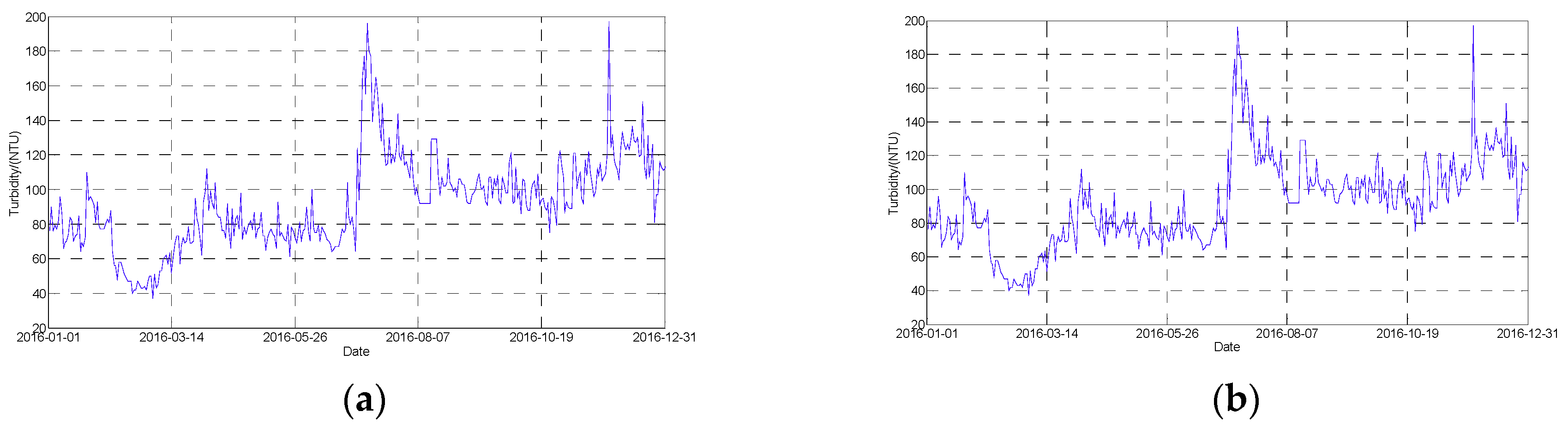
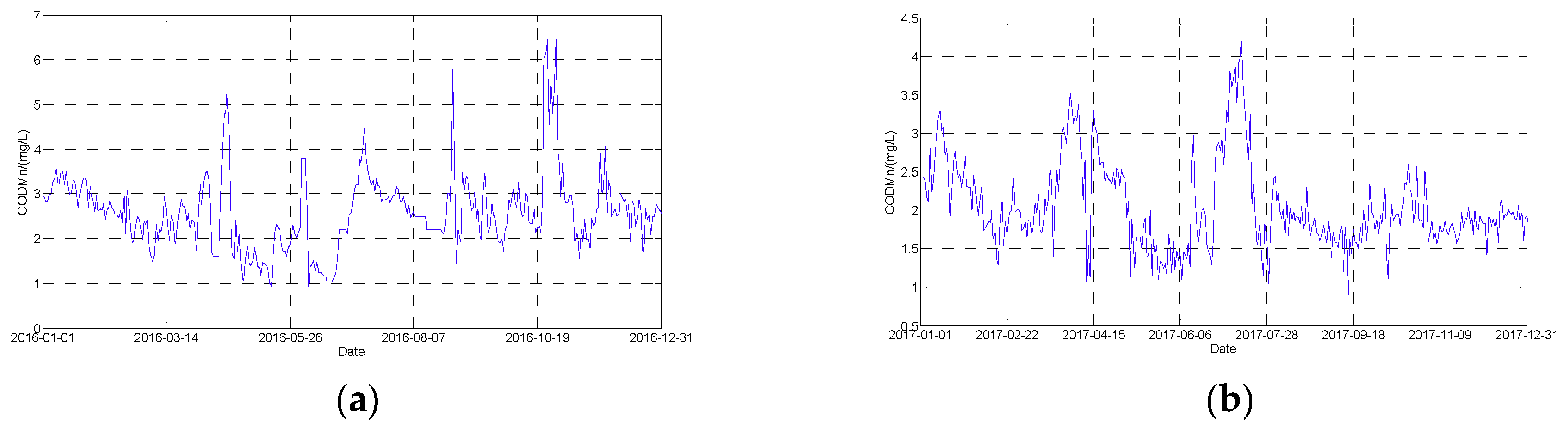
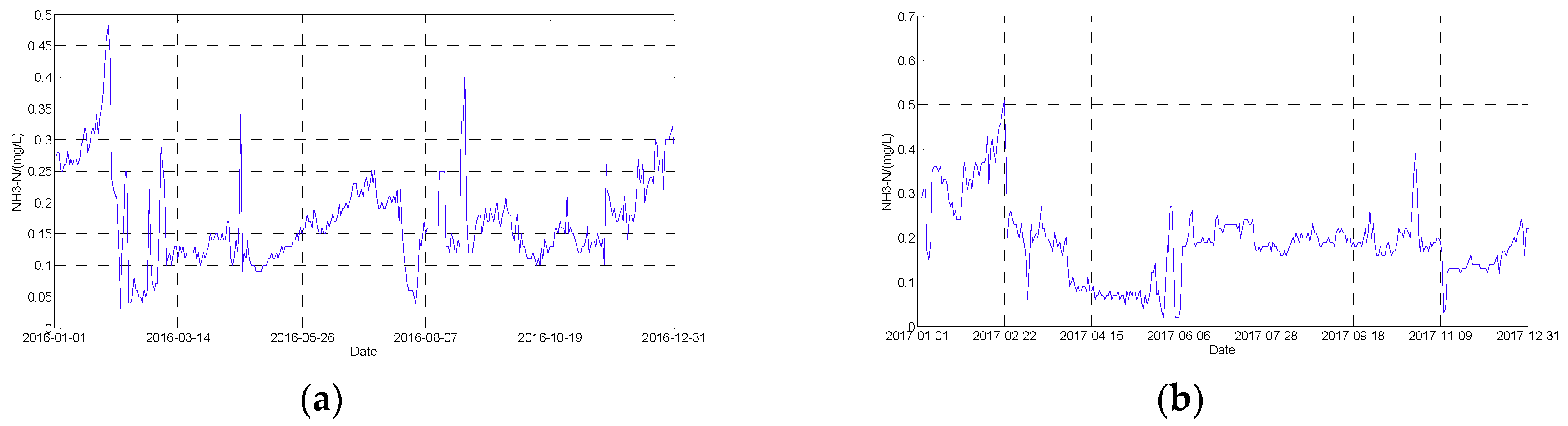
As can be seen from Figure 2, Figure 3, Figure 4, Figure 5, Figure 6 and Figure 7 and Table 1 and Table 2, the pH value in 2016 was maintained between 7.52 and 7.96, while the pH value in 2017 was between 7.75 and 8.33, which was higher than that in 2016. The minimum average values of dissolved oxygen in 2016 and 2017 appeared in July, a very hot month, and the maximum average values of dissolved oxygen in 2016 and 2017 appeared in February, in the winter with low temperature, showing that the value was greatly affected by the water temperature. The minimum average values of CODMn in 2016 and 2017 appeared in May, while the maximum values appeared in July, according to certain rules. The maximum average values of conductivity in 2016 and 2017 appeared in December, and the minimum average values of turbidity in 2016 and 2017 appeared in February. The minimum and maximum average values of NH₃–N were irregular.

In order to deeply analyze the relationship between the awater quality parameters, correlation analysis of water quality parameters was conducted for 731 groups of data collected between 1 January 2016 and 31 December 2017. For the sake of eliminating the influence of dimension, the data were standardized, and Pearson correlation coefficient matrix was acquired. As can be seen from

Table 3. Pearson correlation coefficient matrix of water quality parameters.

Parameters	Water Temperature	pH	Dissolved Oxygen	Conductivity	Turbidity	CODMn	NH3-N
Water Temperature	1.00000	0.24196	−0.93512	−0.30045	0.46194	−0.13766	−0.30422
pH		1.00000	−0.11692	0.66766	0.39667	−0.57278	0.00138
Dissolved Oxygen			1.00000	0.30731	−0.56432	0.00149	0.29651
Conductivity				1.00000	0.17924	−0.48991	0.19584
Turbidity					1.00000	0.27434	−0.00203
CODMn						1.00000	0.11754
NH3-N							1.00000

, the water temperature in Guazhou Water Source of Yangtze River showed a significant relationship with the pH value, dissolved oxygen, conductivity, turbidity, CODMn, and NH₃–N under the 0.01 significant level, showing a positive correlation with pH value and turbidity and a negative correlation with the other parameters. In particular, a high correlation with dissolved oxygen was observed, with a Person value of −0.93512. Dissolved oxygen was negatively correlated with water temperature and turbidity at the significant level of 0.01; the correlation with turbidity was −0.56432, while the correlation with CODMn was not significant. Conductivity was significantly correlated with water temperature, dissolved oxygen, turbidity, CODMn, and NH₃–N at the significant level of 0.01; specifically, conductivity was negatively correlated with water temperature and CODMn, while it was positively correlated with the other parameters, especially, it was highly correlated with pH value, with a Person value of 0.66766. The correlation between NH₃–N and pH value and turbidity was not significant, considering the significant level of 0.01.

2.2. Data Pre-Processing

Water quality automation monitoring stations likely encounter problems, such as missing data and abnormal data during operation, due to sensor failures, network failures, or accidental events (i.e., ships or fish shoal passing by). Data defects will eventually lead to excessive deviation between water quality prediction results and actual monitoring values. To improve forecasting accuracy and to provide clean, accurate, and concise data for predictive models, monitoring data of raw water quality must be processed in advance.

In automatic water quality monitoring system, data are often missing. From the time dimension, the monitored water quality parameters were only monitored once at a certain time. Because the time is irreversible, the missing data can no longer be acquired, so the missing data can only be estimated as accurately as possible. In the current study, the commonly used treatment method was to fill in the missing part of the data and then predict water quality. As long as the method of filling in is appropriate, the results obtained are satisfactory.

The current method of missing value imputation is mainly divided into single imputation (SI) and multiple imputation (MI). The operation of MI is more complicated, and its cost is relatively higher. As illustrated in Figure 2 and Figure 3, the water quality parameters monitored by the automatic water quality monitoring station showed continuous changes in the time dimension, and the monitoring values showed usually certain time correlations. Therefore, this paper used a linear interpolation (LIN) algorithm [23]. On the basis of the temporal correlation of the monitoring data, the algorithm uses a linear imputation model to obtain a better estimation effect for the missing values of the monitoring data in a short time interval.

Definition 1.

Time series of water quality parameters.

Usually, the data set of water quality monitored by the same automatic monitoring station can be regarded as a time series. It is an ordered collection composed of water quality measurement values and measuring times. Supposing an automatic monitoring station measures the water quality parameters at a fixed time every day, and the parameter number is j, we define

$$S_{i,n}=\left(\langle y_{i,1},T_1\rangle ,\dots ,\langle y_{i,n},T_n\rangle \right)$$

(1)

to represent the n-length time series of water quality parameters, where $y_{i,k}$ is the value of the ith water quality parameter measured by the monitoring station at observation time $T_k$ (1 ≤ i ≤ j, 1 ≤ k ≤ n), and, for any $T_k$, the sampling time interval is fixed at $△T=T_{k+1}-T_k$ = 1 (day).

If the observed value $y_{i,k}$ at $T_k$ is missing, then we can obtain its estimated value ${\widehat{y}}_{i,k}$ and change the problem of minimum $\left|{\widehat{y}}_{i,k}-y_{i,k}\right|$ into the missing value estimation problem. For a water quality monitoring station, based on the monitoring data $y_{i,u}$ and $y_{i,v}$ at any $T_{i,u}$ and $T_{i,v}$, the linear imputation function can be constructed as:

$$L\left(t\right)=y_{i,u}+\frac{y_{i,u}-y_{i,v}}{T_{i,u}-T_{i,v}}\left(t-T_{i,u}\right)$$

(2)

When the water quality data at a certain moment is missing, the LIN algorithm will firstly find the two closest moments $T_{i,u}$, $T_{i,v}$ ($T_{i,u}$ < t < $T_{i,v}$) and then estimate the missing value at time t by using the monitoring data $y_{i,u}$ and $y_{i,v}$ of the two moments, based on formula (2), that is, ${\widehat{y}}_n=L\left(t\right)$.

In a word, the LIN algorithm can obtain a good estimation of the missing value in stationary time series in a short period of time, but its estimation of missing values in non-stationary time series is poor [23]. Therefore, for non-stationary time series, we used mean imputation to process the missing data.

3. Water Quality Prediction Model Based on LSTM Deep Neural Networks

3.1. Water Quality Medium- to Long-Term Prediction

Definition 2.

Time series prediction of water quality parameters.

For the n-length time series $S_{i,n}=\left(\langle y_{i,1},T_1\rangle ,\dots ,\langle y_{i,n},T_n\rangle \right)$ of water quality parameters, the prediction period length is defined as m, $m\in$ {1,2,…}. LSTM deep neural networks are used to realize the time-series prediction task and give a new future time series

$$S_{i,n+m}=\left(\langle y_{i,n+1},T_{n+1}\rangle ,\langle y_{i,n+2},T_{n+2}\rangle ,\dots ,\langle y_{i,n+m},T_{n+m}\rangle \right)$$

(3)

Because of the complexity, uncertainty, and lack of relevant information of water quality-influencing factors, the precision of water quality prediction in several medium- to long-term (m = 10 to 365) scales are still not satisfactory, which brings great difficulties to the scientific decision-making of water pollution control and water quality planning and management. Aiming at the problem, we built a prediction model on the basis of LSTM deep neural networks and deeply learned and trained the monitoring data of water quality from the automatic monitoring station of Guazhou Water Source in Yangzhou City in 2016 and 2017 (n = 731), to predict water quality data for the next six months (m = 181). In this way, a more reasonable medium- to long-term water quality prediction method was proposed to improve the accuracy of the medium- to long-term water quality prediction.

3.2. LSTM Networks

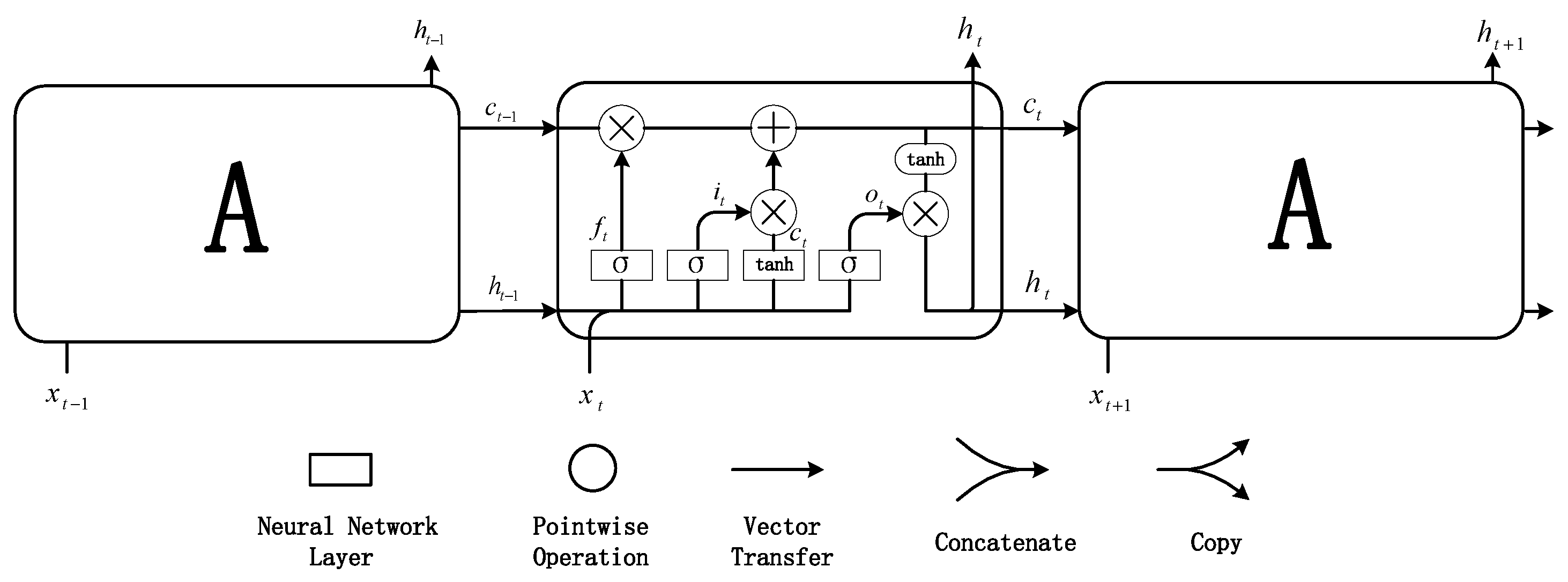
As a special kind of recurrent neural network (RNN), LSTMs have the ability to learn long-term dependencies. All RNNs take the form of chained repeating modules of neural network. LSTMs that use purpose-built memory cells to store information also have this chained in similar structure, but the repeating module is structured differently. As shown in Figure 8, there are four interacting layers in an LSTM cell [24].

In Figure 8, x is the input, h and C are two memory vectors, and C are cell activation vectors, all of which are the same size as the hidden vector h; $\sigma$ is the logistic sigmoid function. The task of tanh is to push the values to be between −1 and 1.

For a start, the “forget gate layer” decides what information we are going to delete from the cell state. Secondly, the “input gate layer” decides which values we will update. Afterwards, a tanh layer creates a vector for the new candidate values $\widetilde{C_t}$. Then, we update the old cell state C_{t − 1} into the new cell state C_t. In the next part, the “output gate layer” decides what parts of the cell state we mean to put out. Finally, we put the cell state through tanh and multiply it by the output gate.

Here are the equations computed by a cell:

• Forget gate layer.

  $$f_t=\sigma \left(w_f·\left[h_{t-1},x_t\right]+b_f\right)$$

  (4)
• Input gate layer.

  $$i_t=\sigma \left(w_i·\left[h_{t-1},x_t\right]+b_i\right)$$

  (5)
• New memory cell.

  $$\widetilde{C_t}=tanh\left(w_f·\left[h_{t-1},x_t\right]+b_f\right)$$

  (6)
• Final memory cell.

  $$C_t=f_t\ast C_{t-1}+i_t\ast \widetilde{C_t}$$

  (7)
• Output gate layer.

  $$o_t=\sigma \left(w_o·\left[h_{t-1},x_t\right]+b_o\right)$$

  (8)

  $$h_t=o_t+tanh\left(C_t\right)$$

  (9)

where w is a matrix, b is the bias, i is the input gate, f is the forget gate, and o is the output gate.

3.3. Water Quality Prediction Model Based on LSTM Deep Neural Networks

As an extended model with multiple hidden LSTM layers, each layer of the stacked LSTM has numerous memory cells, which makes the model earning the deep learning technique [25]. As shown in Figure 9, we designed a water quality prediction model based on LSTM deep neural networks.

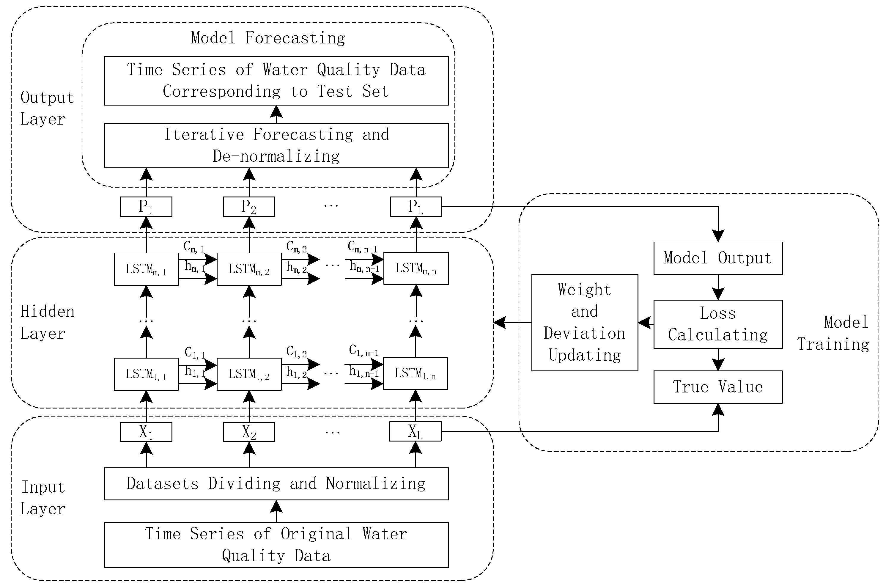
3.4. Workflow of Water Quality Prediction Model Based on LSTM Deep Neural Networks

This paper tried to build a deep neural network architecture using Keras and Tensorflow to provide water quality forecasting by means of Python version 3.6. The whole specific workflow of water quality prediction model based on deep neural networks was as follows:

• Transform and load the water quality data from the CSV file to a pandas dataframe which will then be used to put out a NumPy array that will feed the LSTM.
• Build the LSTM deep neural network model.
• Train the model with training data.
• Run a point-by-point prediction for the output.

If we tried to train the model on the raw data without normalizing, it would never converge because the water quality data is not just in the numerical range of −1 to 1. To solve this problem, we normalized each n-sized list of training/testing data to reflect the percentage changes from the start of the list. The following equation was used for normalizing:

$$n_i=\left(\frac{p_i}{p_0}\right)-1$$

(10)

where n is a normalized list of water quality data, and p is a raw list of adjusted water quality data. At the end of the prediction process, de-normalization was used to get the real water quality data out of the prediction with the following equation:

$$p_i=p_0\left(n_i+1\right)$$

(11)

In terms of step 4, a point-by-point prediction means that we only predict a single point before each time, plot this point as a prediction, then take the next data listed along with the full testing data, and finally predict the next point once again.

4. Experiments

4.1. Model Parameters Configuration

We used the water quality monitoring data from the automatic monitoring station of Guazhou Water Source from January 2016 to December 2017 as the training set (time series length n = 731) and, respectively, predicted the different six parameters in the first half of 2018 (prediction period length m = 181). When performing the LSTM model training, the number of iterations epoch was set to 100. The training sets were grouped by mini-batch gradient descent. After grouping, the gradients were evaluated for each group, and then the parameters were updated. Mean square error (MSE) was chosen as loss function. Adaptive moment estimation (Adam), which has a good effect in practical applications, was adopted as the LSTM model optimization algorithm, and the model update weight and the deviation parameters were adjusted. We set 100 neurons in each LSTM layer.

4.2. Water Quality Prediction Effects

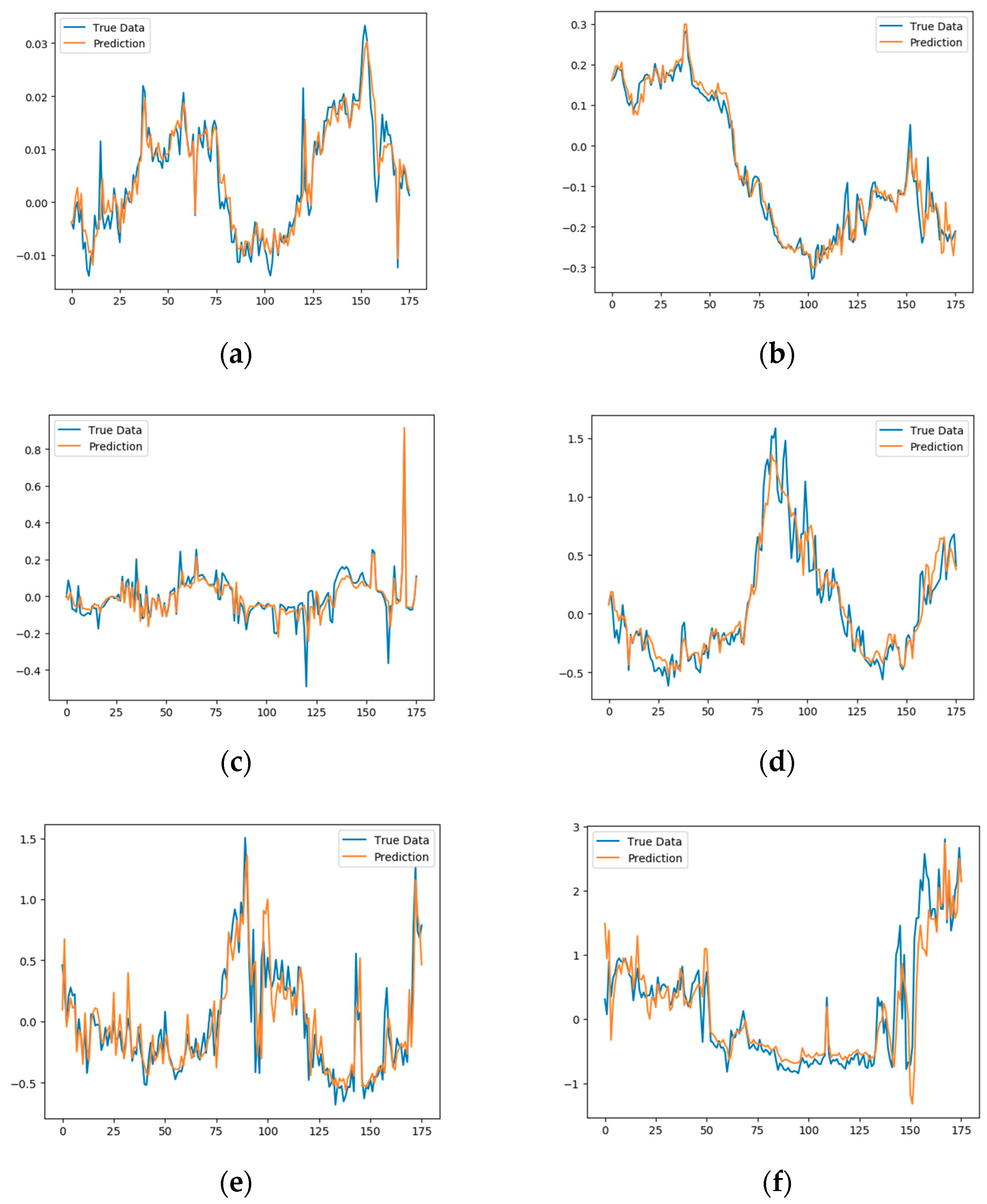
Taking the training set as a learning sample, deep learning and training were carried out. We took the actual monitoring data of 1 January 2018 to 30 June 2018 as the test set and compared the predicted results with the actual monitoring data. The results are shown in Figure 10.

We concluded that the predicted values had a good agreement with the effective values of the model, indicating that this model performed well in predicting the water quality parameters (Figure 10). Our result reveals the potential of applying LSTM and deep learning to predict drinking water quality, which can provide a reliable foundation for the formulation for water source protection policies and concrete measures.

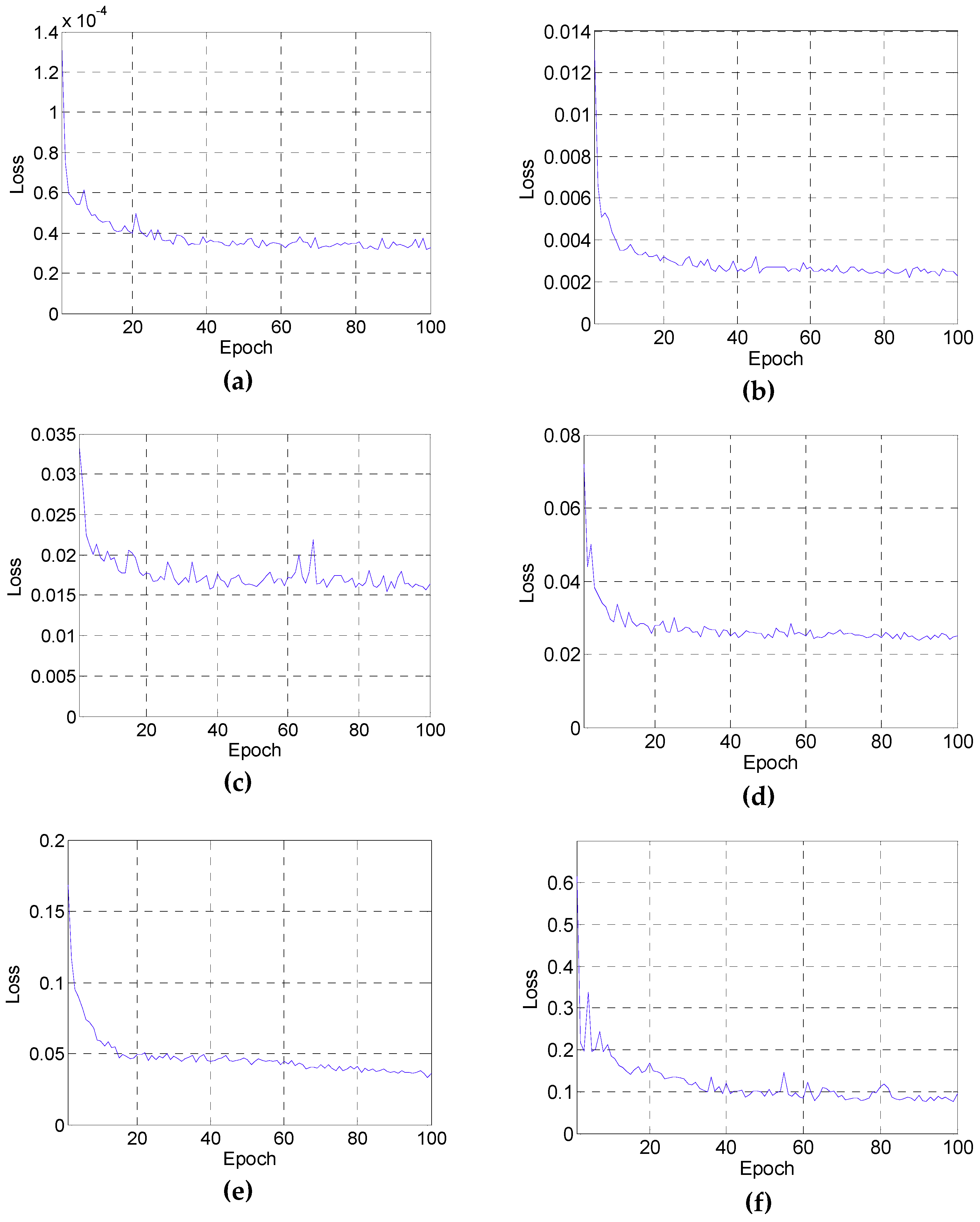
In the course of predicting various water quality parameters, we recorded the values of loss function after each iterating and drew the change trend diagrams of loss function with respect to the number of iterations epoch, as shown in Figure 11. A loss is a “penalty” score to reduce when training an algorithm on data. It is usually called the objective function to optimize. Drinking-water quality prediction pursues the accuracy of prediction results and the stability of prediction error fluctuation. In our model, MSE was used to evaluate the degree of fitting between the predicted values and the actual values in the model analysis. The smaller MSE is, the lower the dispersion degree between the predicted values and the true values is, and the more reliable the predicted result will be [12]. As can be seen from Figure 11, after each round of whole training, the value of loss function always kept a decreasing trend and decreased less after a certain period of time, demonstrating that the learning outcome of this model was good.

4.3. Contrastive Models

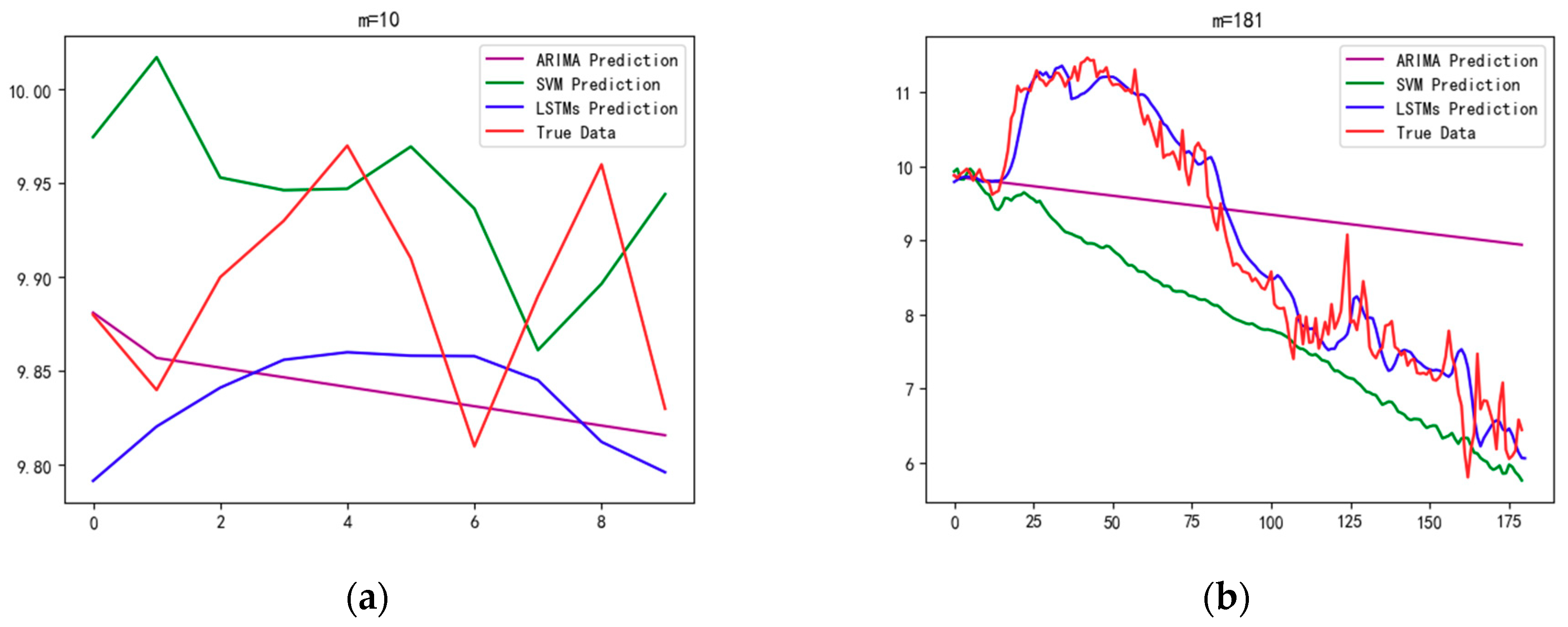
In order to verify the prediction effect of our model based on LSTM deep neural networks in depth, this paper compared the model with two other classical time-series prediction models, autoregressive integrated moving average (ARIMA) and support vector regression (SVR). We used a set of 731 dissolved oxygen data monitored by the Guazhou automatic water quality monitoring station in 2016 and 2017 as the training set (n = 731) and respectively predicted the dissolved oxygen data in the next 10 days (m = 10) and the next 6 months (m = 181). For model prediction accuracy, MSE was chosen as the unified metrics. The experiment results are shown in Figure 12 and

Table 4. Comparison of the prediction accuracy of the three models. ARIMA, autoregressive integrated moving average, SVR, support vector regression.

Model	MSE Values
	Prediction Period Length m = 10	Prediction Period Length m = 181
ARIMA	0.0126	2.4326
SVR	0.0046	1.9943
LSTMs	0.0017	0.0020

.

The ARIMA model can be expressed as ARIMA (p, d, q), and, in the ARIMA modeling process, we determined the values of the three parameters by calculating the Bayesian information criterion (BIC) value. After tuning the parameters, we found that when the BIC value was the minimum, p = 0, d = 1, and q = 2.

In the SVR model, the frequently used Gaussian RBF was chosen as the nonlinear kernel function, and the kernel function parameter σ was set to 0.001. If m = 10, we set the penalty factor C to 100, while if m = 181, we set C to 10.

Compared with the other two prediction models, the dissolved oxygen prediction precision of our model was higher, no matter if it was for short-term or medium- to long-term predictions. Especially, when the prediction period length m = 181, the dissolved oxygen precision of our model was obviously superior to those of ARIMA and SVR. Besides, it can be seen in Figure 11b that our model converged quickly. Furthermore, with the same amount of data as those of the training set, under ARIMA and SVR, the prediction of dissolved oxygen in the next six months would become inaccurate because of the too long prediction period, whereas LSTM deep neural networks would still work well, with only a relatively small training set of data.

5. Conclusion and Future Work

Combined with the analysis and pretreatment of the water quality data collected by the automatic water quality monitoring station of Guazhou Water Source of the Yangtze River in Yangzhou, this paper proposes a water quality forecasting method with the help of LSTM deep neural networks and establishes the sample, data pre-processing, parameter setting, and learning procedure of LSTM deep neural networks. The established prediction model can be trained and learned automatically in the face of different water quality data samples and thus has broad application scenarios. The result shows that the built water quality model can predict the drinking-water quality in the future 6 months well, offering a feasible approach for water quality prediction.

Our model only considered single dimensional inputs, while there are more complex datasets with many different dimensions for sequences in water quality monitoring. Our future work will focus on the model optimization by combining the various water quality parameters, and multi-dimensional input datasets will be used to predict the target parameters, so as to improve the accuracy of the model. Besides, the present research predicted the drinking-water quality data in one monitoring station in Guazhou of the Yangtze River, and, for future research, we will take into account three monitoring stations in the Yangzhou section of the Yangtze River (Guazhou, Shierwei, Xiaohekou of Yizheng) to predict the water quality data, making predictions of water quality in spatial dimensions under the hydrodynamic principle.

References

- Tirkolaee, E.B.; Hosseinabadi, A.A.R.; Soltani, M.; Sangaiah, A.K.; Wang, J. A Hybrid genetic algorithm for multi-trip Green Capacitated Arc routing problem in the scope of urban services. Sustainability 2018, 10, 1366. [Google Scholar] [CrossRef]
- Mishra, D.R.; D’Sa, E.J.; Mishra, S. Preface: Remote sensing of water resources. Remote Sens. 2018, 10, 115. [Google Scholar] [CrossRef]
- Gleason, C.J.; Wada, Y.; Wang, J. A hybrid of optical remote sensing and hydrological modelling improves water balance estimation. J. Adv. Model. Earth Syst. 2017, 10, 2–17. [Google Scholar] [CrossRef]
- Ren, Y.; Liu, Y.; Ji, S.; Sangaiah, A.K.; Wang, J. Incentive mechanism of data storage based on blockchain for wireless sensor networks. Mob. Inf. Syst. 2018, 2018, 6874158. [Google Scholar] [CrossRef]
- Yin, C.; Xi, J.; Sun, R.; Wang, J. Location privacy protection based on differential privacy strategy for big data in industrial internet of things. IEEE Trans. Ind. Inform. 2018, 14, 3628–3636. [Google Scholar] [CrossRef]
- Wang, J.; Ju, C.; Gao, Y.; Sangaiah, A.K.; Kim, G.-J. A PSO based energy efficient coverage control algorithm for wireless sensor networks. Comput. Mater. Contin. 2018, 56, 433–446. [Google Scholar]
- Wang, J.; Gao, Y.; Yin, X.; Li, F.; Kim, H.-J. An enhanced PEGASIS algorithm with mobile sink support for wireless sensor networks. Wirel. Commun. Mob. Comput. 2018, 2018, 9472075. [Google Scholar] [CrossRef]
- Wang, J.; Cao, J.; Sherratt, R.S.; Park, J.H. An improved ant colony optimization-based approach with mobile sink for wireless sensor networks. J. Supercomput. 2018, 74, 6633–6645. [Google Scholar] [CrossRef]
- Zheng, J.; Jiao, J.; Liping Sun, L. A modeling approach for early-warning of water bloom risk in urban lake based on neural network. China Environ. Sci. 2017, 37, 1872–1878. [Google Scholar]
- Li, X.H.; Ding, Y.; Si, A. Application of fuzzy comprehensive evaluation model in groundwater quality evaluation—A case study in Baodi. Ground Water 2014, 1, 6–8. [Google Scholar]
- Liu, S.; Tai, H.; Ding, Q.; Li, D.; Xu, L.; Wei, Y. A hybrid approach of support vector regression with genetic algorithm optimization for aquaculture water quality prediction. Math. Comput. Model. 2013, 58, 458–465. [Google Scholar] [CrossRef]
- Zhang, C.C.; Chen, Q.W.; Xu, Q.; Zhang, X. A chlorophyll a prediction model for meiliang bay of Taihu based on support vector machine. Acta Scientiae Circumstantiae 2013, 33, 2856–2861. [Google Scholar]
- Theo, W.; Wong, S.H.C.; Choi, K.W.; Lee, J.H.W. Daily prediction of marine beach water quality in Hong Kong. J. Hydro Environ. Res. 2012, 6, 164–180. [Google Scholar] [CrossRef]
- Gazzaz, N.M.; Yousoff, M.K.; Aris, A.Z.; Juahir, H.; Ramli, M.F. Artificial neural network modeling of the water quality index for Kinta River (Malaysia) using water quality variables as predictors. Mar. Pollut. Bull. 2012, 64, 2409–2420. [Google Scholar] [CrossRef]
- Liu, D.J.; Zou, Z.H. Application of weighted combination model on forecasting water quality. Acta Scientiae Circumstantiae 2012, 32, 3128–3132. [Google Scholar]
- Clark, R.; Hakim, S.; Ostfeld, A. Handbook of Water and Wastewater Systems Protection (Protecting Critical Infrastructure); Springer: New, York, NY, USA, 2011. [Google Scholar]
- Maier, H.R.; Jain, A.; Dandy, G.C.; Sudheer, K.P. Methods used for the development of neural networks for the prediction of water resource variables in river systems: Current status and future directions. Environ. Model. Softw. 2010, 25, 891–909. [Google Scholar] [CrossRef]
- Sangmok, L.; Donghyun, L. Improved prediction of harmful algal blooms in four major South Korea’s rivers using deep learning models. Int. J. Environ. Res. Public Health 2018, 15, e1322. [Google Scholar]
- Storey, M.V.; van der Gaag, B.; Burns, B.P. Advances in on-line drinking water quality monitoring and early warning systems. Water Res. 2011, 45, 741–747. [Google Scholar] [CrossRef]
- Yesilnacar, M.I.; Sahinkaya, E.; Naz, M.; Ozkaya, B. Neural network pre-diction of nitrate in groundwater of Harran Plain, Turkey. Environ. Geol. 2008, 56, 19–25. [Google Scholar] [CrossRef]
- Bouamar, M.; Ladjal, M. A comparative study of RBF neural net-work and SVM classification techniques performed on real data fordrinking water quality. In Proceedings of the 5th International Multi-Conference on Systems, Signals and Devices 2008, Amman, Jordan, 20–22 July 2008; pp. 1–5. [Google Scholar]
- Huang, C.-J.; Kuo, P.-H. A deep CNN-LSTM model for particulate matter (PM2.5) forecasting in smart cities. Sensors 2220, 18, 2220. [Google Scholar] [CrossRef]
- Pan, L.; Li, J.; Luo, J. A temporal and spatial correction based missing values imputation algorithm in wireless sensor networks. Chin. J. Comput. 2010, 33, 1–10. [Google Scholar] [CrossRef]
- Christopher Olah. Understanding LSTM Networks. 27 August 2015. Available online: http://colah.github.io/posts/2015-08-Understanding-LSTMs/ (accessed on 26 December 2018).
- Jason Brownlee. Stacked Long Short-Term Memory Networks Develop Sequence Prediction Models in Keras. 18 August 2017. Available online: https://machinelearningmastery.com/stacked-long-short-term-memory-networks/ (accessed on 19 January 2019).
Figure 1.
Locations of partial water quality automatic monitoring stations in Yangzhou water source area.
Figure 2.
Graphs of the pH variation trend of Guazhou Water Source. (a) pH variation trend in 2016, (b) pH variation trend in 2017.
Figure 3.
Dissolved oxygen variation trend of Guazhou Water Source. (a) Dissolved oxygen variation trend in 2016, (b) dissolved oxygen variation trend in 2017.
Figure 4.
Conductivity variation trend of Guazhou Water Source. (a) Conductivity variation trend in 2016, (b) conductivity variation trend in 2017.
Figure 5.
Turbidity variation trend of Guazhou Water Source. (a) Turbidity variation trend in 2016, (b) turbidity variation trend in 2017.
Figure 6.
Chemical oxygen demand (CODMn) variation trend of Guazhou Water Source. (a) CODMn variation trend in 2016, (b) CODMn variation trend in 2017.
Figure 7.
NH3–N variation trend of Guazhou Water Source. (a) NH3–N variation trend in 2016, (b) NH3–N variation trend in 2017.
Figure 8.
Long short-term memory (LSTM) structure.