The Modified Artificial Fish Swarm Algorithm for Least-Cost Planning of a Regional Water Supply Network Problem

1
Management School, Hangzhou Dianzi University, Hangzhou 310018, China
2
The Research Center of Information Technology & Economic and Social Development, Hangzhou Dianzi University, Hangzhou 310018, China
*
Author to whom correspondence should be addressed.
Sustainability 2019, 11(15), 4121; https://doi.org/10.3390/su11154121
Submission received: 1 July 2019
/
Revised: 23 July 2019
/
Accepted: 24 July 2019
/
Published: 30 July 2019
Abstract
:A regional water supply network (RWSN) plays a key role in the process of urbanization development. This paper researches the planning optimization model of a regional water supply network with the payoff characteristic between economical cost and reliability, in which the hydraulic-connectivity is selected as the surrogate measure of the reliability in the regional water supply network. The modified artificial fish swarm algorithm (MAFSA) is proposed to solve the optimization problem by adjusting research visual and the inertia weights of artificial fish swarm algorithm (AFSA) according to the hydraulic-connectivity. The experiment results of regional water supply network show that MAFSA can effectively obtain the optimal solution with the maximum reliability and least cost compared to other algorithms, which can thereby achieve the optimization of RWSN engineering applications.
1. Introduction
The regional water supply network (RWSN) (mainly including water intake project, water purification project and pipeline network subsystem) are typically part of an aging infrastructure, which faces challenges to efficiently and sufficiently serve a growing population and urbanization development under more stringent economic and environmental constraints. The water distribution network is the largest investment of the regional water supply system, which the optimal planning of water supply network affects the economy and reliability of the regional water supply networks [1]. The planning of the regional water supply network is a complicated project involving the scale of pipe network, initial flow distribution, pipelines, and so on [2]. Therefore, the optimal planning of the RWSN will influence the investment in the regional water supply system, which can safely and reliably transport water to every demand node of the network through water distribution pipelines.
The traditional optimization methods for the water supply network are those that distribute the flow of the pipe section firstly, then determine the diameter of the pipeline base on the flow rate, and make the hydraulic calculation according to the diameter of the pipeline, and finally obtain the water tower height and the pump head. The traditional method only considers the minimal cost for pipe laying under hydraulic conditions. However, the optimal design scheme of water supply network system can meet the actual project requirements for water quantity, water quality and hydraulic pressure, which have great practical significance for reducing energy consumption and promoting social and economic benefits. Therefore, this paper will formulate the multi-objective function subject to the supply, demand, reliability, and economic constraints, whose reliability means that the water amount and water pressure is enough for consumers under the abnormal condition, and the economics of the network is the optimal layout of the pipeline network in the case of hydraulic conditions. The formulated optimization problem is solved using the computer-aided tool Xpress Optimizer (Version 8.6, FICO, San Jose, CA, USA) to determine the design, capacity, and location of the regional water supply network.
2. Literature Review
Shin and Park (2000) established the optimization model of a regional water supply network with the objective function of the minimal construction cost, and used the genetic algorithm to design the network connection of pipe section [3]. Wu and Simpson (2005) constructed the optimization model of a regional water supply network and used the adaptive genetic algorithm to solve the multi-objective optimization problem, including the minimal construction cost of the pipeline, pump station, water tank and pipe nodes [4]. Junfei Qiao (2011) established the non-linear optimization model with the single economical objective function and used the particle swarm optimization algorithm to design the water supply network [5]. Savic et al. (2000) established the multi-objective function for the optimal design of the water supply system considering the velocity, pressure and loss of water supply pipeline as the constraints, used the genetic algorithm to solve this multi-objective optimization problem, and obtained better results [6]. Vasan et al. (2010) established the multi-objective function including the hydraulic reliability and economic performance, used the modified genetic algorithm for the water supply network, and achieved better results, which has been applied for the actual pipeline network project of a Moroccan city [7]. Beyond the implicit non-linearity, the number of parameters involved in the hydraulic equations (Abraham and Stoianov 2015) [8] and their large number of possible combinations introduce high complexity to the RWSN problem (Takahashi et al. 2010) [9]. For large RWSN, these have an expensive computational cost since, even for moderate-sized networks, which is an NP (non-deterministic polynomial) problem, cannot be solved in polynomial time (Berardi et al. 2014) [10]. Traditional mathematical optimization methods, such as linear programming (LP) [11], non-linear programming (NLP) [12] and dynamic programming (DP) [13] often have drawbacks obtaining the satisfied optimal planning schemes of large-scale pipeline networks in practice, which the various meta-heuristic optimization techniques have been developed to overcome these drawbacks.
The artificial fish swarm algorithm (AFSA) is the swarm intelligent (SI) optimization algorithm with multi-point parallel random search manner, which has the characteristics of robust, positive feedback and easy integration with other methods [14]. The artificial fish swarm algorithm simulate the fish swarm’s behaviors of preying, clustering, chasing and randomness in the evolutionary process. Prey behavior is the basic operation. When discovering food nearby, the fish will swim in that direction. Cluster behavior often form the large group movement. Chase behavior indicates that one fish finds rich food and others follow it. Random behavior allows fish to swim freely. The parameters of AFSA are as following, each artificial fish represents the solution Xi = (x1, x2, …, xn) (i = 1, 2, …, n), N is the number of artificial fishes, the objective function Y = f(Xi) is the food density of artificial fish Xi, the visual scope is the search field of AFSA, the search step is the maximum move length, Disi,j = Dis(xi, xj) (i,j = 1, 2, …,n) is the distance between fish Xi and Xj, the congestion factor δ(0 < δ < 1) is the crowd factor adjusting the congestion of AFSA. The optimization behaviors of artificial fish swarm algorithm can be described as follows:
Prey behavior: the artificial fish prey at more places of food. The artificial fish xi, will select the state xj randomly in the visual according to the food concentration. If f(xi) < f(xj), the artificial fish will move to xj. The next state xnext of artificial fish can be calculated as follows:
Otherwise, the process selects new state xj again within the distance., If it still cannot find xj according to the f (xi) < f(xj) after attempting to try a number of times, the artificial fish will execute another behavior.
Swarm behavior: the artificial fishes often form the large group. This behavior should follow two principles: one is that the artificial fish will swim toward the center of its fellows around; the other is the swarm should avoid being over-crowded. The nf is the number fellows within visual scope of xi artificial fish. If nf/N < δ (0 < δ < 1), then the swarm is not a crowd. After comparing the food concentration at xi and the center of its fellows xc, if f (xi) < f(xc) then the artificial fish will swim towards to xc. Otherwise, the artificial fish execute another behavior.
Cluster behavior: this behavior means that the swarm of fish will follow the best fish finding more food. If the artificial fish is at xi, and fish swarm within its visual scope is at xmax, compared the food concentration at xi and xmax.
If f(xi) < f(xmax) and nf/N < δ(0 < δ < 1), then the food concentration at xmax is higher and the swarm is not a crowd. So the artificial fish will swim toward the xmax. Otherwise, the artificial fish executes other behavior.
Random roam behavior: each artificial fish will make the random searching process, which is helpful for getting rid of the local optimum. The next state of artificial fish is xnext:
The individual artificial fish will choose different behaviors according to the perception from information of its environment. The artificial fish of AFSA searches the local solution within its visual scope, and the global optimal solution will be found by the cooperation of the fish swarm.
The performance of AFSA relies on the properties of visual scope, congestion factor, search step. This paper proposes the modified artificial fish swarm algorithm (MAFSA) by adjusting the parameters and the dynamic evaluation strategy, which can efficiently obtain the optimal solutions of the water supply network problem.
Compared with traditional optimization algorithms, the artificial fish swarm algorithm (AFSA) has parallel computational ability and adaptive ability to search a global optimal solution, which is fit for solving the NP hard problem and has been widely used in many fields.
3. Methodology
3.1. The Problem Statement for Least-Cost Planning of Regional Water Supply Network Problem
3.1.1. Model Description
For the planning optimization of a RWSN, four aspects should be considered: the water quantity, water pressure, reliability and economy. The traditional network optimization model only considers the economy, which means to get the minimal cost for pipe laying under the hydraulic conditions. Based on the classical optimization model, this paper constructs the multi-objective function integrated reliability and economical targets, whose reliability is to provide enough water and water pressure under the abnormal condition; the economical target is to get the least-cost layout of pipeline network.
3.1.2. Mathematical Formulation
Under the condition that the pipe network layout, water pressure of the water source, water requirement of nodes, minimum water pressure requirement and optional standard pipe diameter specification are known, the optimal planning of a regional water supply pipe network is to seek a set of optimal pipe diameter combinations which can meet the pressure demand of node flow and the minimum cost of water pipeline network [15]
In Equation (3), W is the annual conversion cost of the pipe network, J is the number of pipelines, H0 is the node free head, Qtot is the total flow of the pipe network or the flow of the pump station, Hj is the head loss of the pipe section j. P is the percentage of the cost of maintenance and annual depreciation of the pipe network, which is calculated according to the construction cost of the pipe network. LM is the collection of pipes belong to any pipeline from pump station to control point M, K pipeline is an economical index related to pumping cost, Dj and lj are the diameter and length of pipe j respectively, (A/P, I, T) is the capital recovery factor. Its formula is: I(1+I)T/[(1 + I)T−1], Among them, T is the lifespan of the pipe network and I is the expected rate of return. is the cost of pipe construction per length (including the cost of pipes and buried pipes), where a, b and α are the statistical parameters of the cost per length of pipeline.
The objective function of the pipe network optimization is based on the series of constraint equations, and the hydraulic constraints are as follows:
Flow node continuity constraints:
In Equation (4), Qj is the flow of node j, and qij represents the flow of pipeline connected with node i, where i and j are the starting and ending node numbers of the segment. Each node in the pipe network should satisfy the continuity equation.
Energy balance constraints:
In Equation (5), Hj is the free head loss of the pipeline base ring. Energy balance constraints are also called loop constraints. The algebraic sum of head loss is zero in the closed loop.
Node pressure constraints:
where Hj is the water pressure of the jth node.
Diameter constraint:
In Equation (7), Dj is the standard diameter set and min is the minimum diameter. In the optimization design of the pipe network, the selection of pipe diameter must be within the standard discrete pipe diameter in the market, and be larger than the minimum required pipe diameter.
Flow velocity constraint:
If the velocity of the water flow is too slow, residual chlorine will precipitate and the chlorine concentration of the end pipeline will decrease. Therefore, the minimum velocity of water flow is set. If the current velocity is too fast, a water accident will occur. Therefore, the upper limit of the velocity is set.
Water supply constraints:
The maximum water consumption of each pipeline network should be equal to the supply quantity of the water resource, and each pipeline should satisfy the constraints of the minimum hydraulic quantity and the maximum capacity of the water supply.
3.2. The Modified Artificial Fish Swarm Algorithm (MAFSA) for the Regional Water Supply Network (RWSN) Problem
3.2.1. Initialization of Artificial Fish Swarm Algorithm
The modified AFSA algorithm solves the problems of a water supply network, whereby the artificial fish will follow the pre-set number of the pipeline network one by one to choose the proper pipe. The initial state of artificial fish X is {X1, X2, X3, …, Xi} (I = 1, 2, …, n), in which each individual fish expresses the element numbers in the solution of the effective scheduled paths. The artificial fish individual adopts integer coding by each diameter of pipe (such as {2 cm, 4 cm, 6 cm, 8cm, 10 cm, 12 cm, 20 cm}),which will assigned in the fish swarm Xi = {X1, X2, …, Xn}, such as Xi = {1-5-2-4-6-3-7} to represent the required diameter. When the fish is in pipeline i, it will use the fitness function FC = f(Xij) to calculate the probability that choose the diameter of pipe j, where xi is optimization variable, Dij = ‖Xi − Xj‖(i,j = 1, 2, …, n) express the distance between fish xi and xj, δ is congestion factor (0 < δ < 1), try number is the maxi-attempt number of artificial fish. Visual is the search scope of artificial fish, N = {Xj|dij < Visual} is the search neighborhood.
3.2.2. Dynamic Swarm Behavior Based on the Isobaric Line of Pipeline Network
In order to display the distribution of hydraulic pressure, it is necessary to draw an isobaric hydraulic chart according to the pressure of each node during the planning of regional water supply network, in which the isobaric line is evenly distributed and the hydraulic gradient of each pipeline within the reasonable range. If the hydraulic pressure line is dense, then the hydraulic gradient is sharp and the pressure of the pipeline is heavy. On the contrary, if the water pressure line is sparse, then the hydraulic gradient is inclined and the pressure of the pipeline is light [16].
Assumed the coordinates of (X1,Y1,H1), (X2,Y2,H2) are the starting point and the end point of the pipeline, where X, Y are coordinate value and H is hydraulic level value, then the hydraulic pressure of the first equivalence point is:
where int (X) is the standard function. The hydraulic pressure of the last equivalent point is:
The middle equivalent point is the integer between Pmax and Pmin. Because the pipeline of the network has a standard calculated flow, the loss pressure of the head is proportional to the length of the pipeline. The coordinates of each isobaric points can be calculated according to the proportionality between the hydraulic pressure of the isobaric points on the pipeline network. The coordinates of the Pi equivalent point can be obtained through Equation (12).
Take the above method to search for equivalent points of each root pipeline. The hydraulic isopiestic line of the whole pipe network is drawn, though the line of the equivalent points surround adjacent segments. Dynamically adjust the searching visual and moving step of the modified AFSA according to the Equation (13).
3.2.3. The Information-Oriented Preying Behavior
The constraints of energy, flow velocity and hydraulic pressure of pipeline should be considered in the optimization of water supply network. The hydraulic loss of pressure hij and closure error of flow node Qij can be calculated according to the Hazen-Williams equation [17].
where, L is the length of pipeline, C is the Hazen William’s coefficient, D is the pipe diameter.
If Ei and Ej are the pressure of ith and jth node, then:
Equation (15) mean the relationship between hydraulic pressure of node and loss of pipeline head, Equation (14) mean the relationship between hydraulic pressure of node and pipeline flow. Equation (17) is as follows:
SGN is the symbolic function:
The new state of Xj is randomly selected from neighborhood within visual. If the fitness of Xj is better than that of current state Xi, then the modified AFSA changes search direction according to Equation (18), which can improve the optimization convergence of the AFSA. The swarm behavior of the modified AFSA algorithm can be represented as Equation (19):
The Xi, is the current state the Xinext is next state of artificial fish, Rand () is the random number within [0, Step]. If the fitness FCj of Xj is better than FCi of Xi, then it moves one step in this direction. Otherwise, else that the new state Xj is selected randomly.
3.2.4. Clustering Behavior
The modified AFSA algorithm should follow two rules during the clustering behavior: 1) move to the center of the neighboring partner as far as possible; 2) avoid overcrowding.
Rule 1: If Xi is the current state of artificial fish, and Nf is the partner number within visual scope, then Xck is the center of Xi neighborhood, as in Equation (20).
Rule 2: Setting the crowding factor . If indicates that the center position Xckß has more food and is not crowded, the fish swarm make cluster to the center according to Equation (21), or else the artificial fish will perform chasing behavior.
3.2.5. Chasing Behavior
Xi is the current state of artificial fish, Xmax is the best state of artificial fish set in the neighborhood. If FCmax > FCi and nf/N < δ, then it will chase towards partner Xmax where they have more the food and are not too crowded, or else adopt preying behavior.
3.2.6. Random Behavior by Competition Mechanism
In order to enhance the searching ability of modified AFSA, the optimal individual Xgbest of artificial fish is retained. When the modified AFSA has minimal change in the search process, the artificial fish algorithm will perform mutation operations with the optimal individual Xgbest using the Hardy–Cross method [18].
where Xi and Xj are random selected artificial fish individuals (i ≠ j), τ is random number within [0,1]. If the offspring is better than the parent, then is replaced by Xgbest.
3.2.7. The Termination Conditions of the MAFSA Algorithm
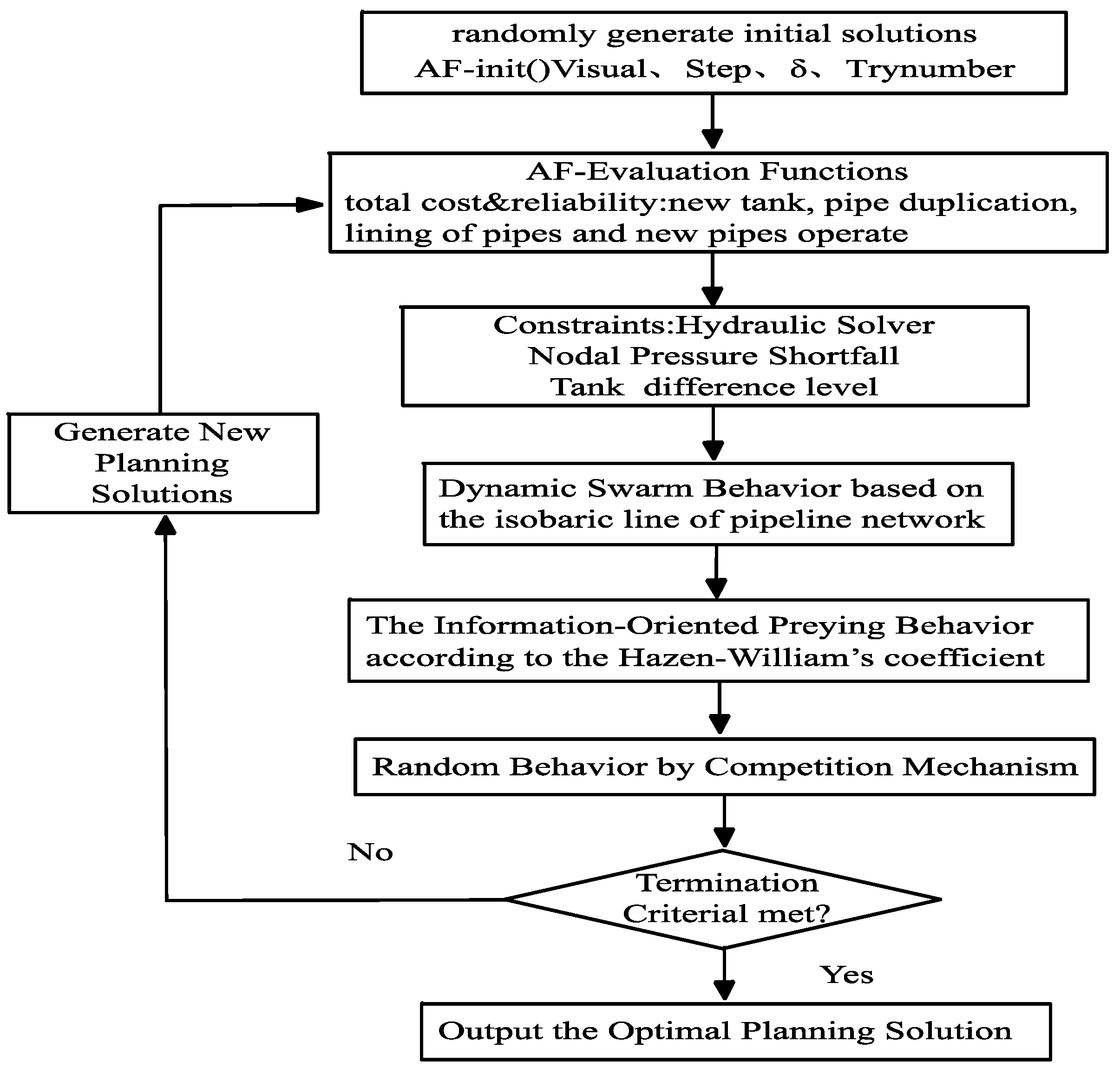
If the maximum iteration number or the optimal solution within the satisfactory bound has been reached, then the MAFSA algorithm terminate and output the optimal solution, otherwise the algorithm return to step 3 and continue the Swarm behavior. The optimization procedure of MAFSA is shown in Figure 1.
4. Case Study and Discussion
4.1. Benchmark Experiment
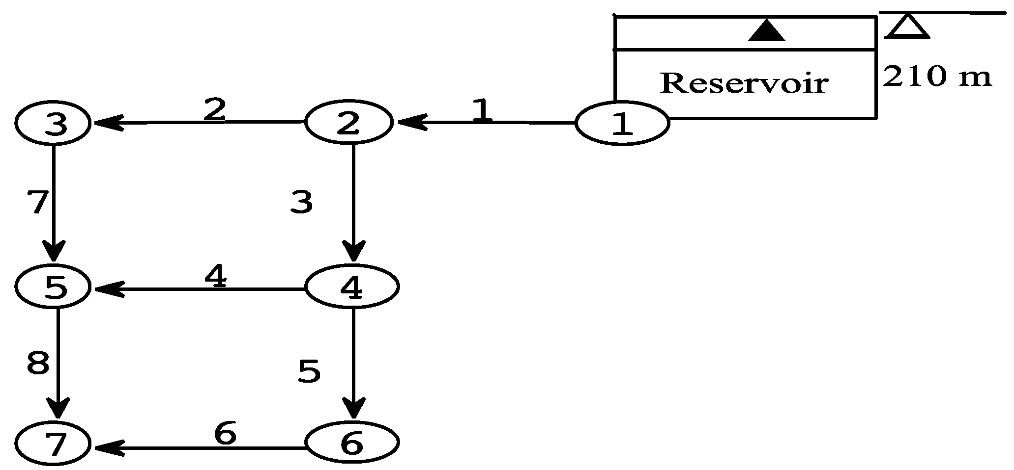
The benchmark experiment is two-loop network studied by Keedwell and Khu 2005 [19]. The two-loop network consists of a reservoir, seven nodes and eight pipelines, which are fed from a single fixed head reservoir to supply the demands as shown in Figure 2 where node 1 is the reservoir. The hydraulic head requires all the demand nodes at 30 m above the elevation, the source water is 210 m, the equal length of each pipeline is 1000 m, water flow is 1120 m3/h. Table 1 and Table 2 show the list of all 12 available pipe sizes and their unit costs. The hydraulic calculation method is used for the planning of the pipeline network, and the Hazen William’s coefficient is taken as C = 130 for all pipes.
The parameters of MAFSA are as follows: the artificial fish population is 100 placed in the source of water distribution network, the maxi- iterations number is 200, the visual scope is 0.5, the try number is 5, the congestion factor δ is 0.8. Considering the algorithm’s schedule efficiency, the artificial fish swarm is coded as natural number according to the pipe diameter; set the pheromone of every pipe diameter as constant τ = 10.67. If the τ is larger, then the water head loss will become larger, which will increase the cost of pipeline in the design scheme. The modified AFSA are implemented in C++ (Bell Labs, Murray Hill, NJ, USA). All the tests were run on the computer with CPU Intel (R) Core (TM) i7-7500U (Intel, Santa Clara, CA, USA), with 16 gigabytes RAM and using the Xpress Optimizer Version 8.6 with the default options. The results of pipeline network optimization are shown in Table 3.
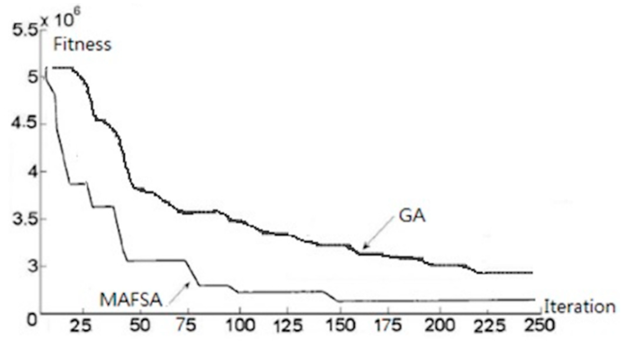
Savic [20] used GA to solve the problem and got the lower cost scheme of 0.420 million, which the hydraulic pressure of each node meets the requirement of 294 kPa. The MAFSA obtained the lowest cost of water distribution network 0.419 million, which all nodes meet the constraint Equations (4)–(9). Compared with the Savic, the modified AFSA can obtain the same results of the pipe network and satisfy the hydraulic pressure of 30 m. Figure 3 shows that the modified AFSA algorithm can obtain the optimal solution in the 75th iteration, and the convergence speed is higher than that of the genetic algorithm [21]. The simulation results show that the modified AFSA algorithm with dynamic intelligent search mode is effective suitable for the design of the water supply network.
4.2. Case Study of Water Distribution Network
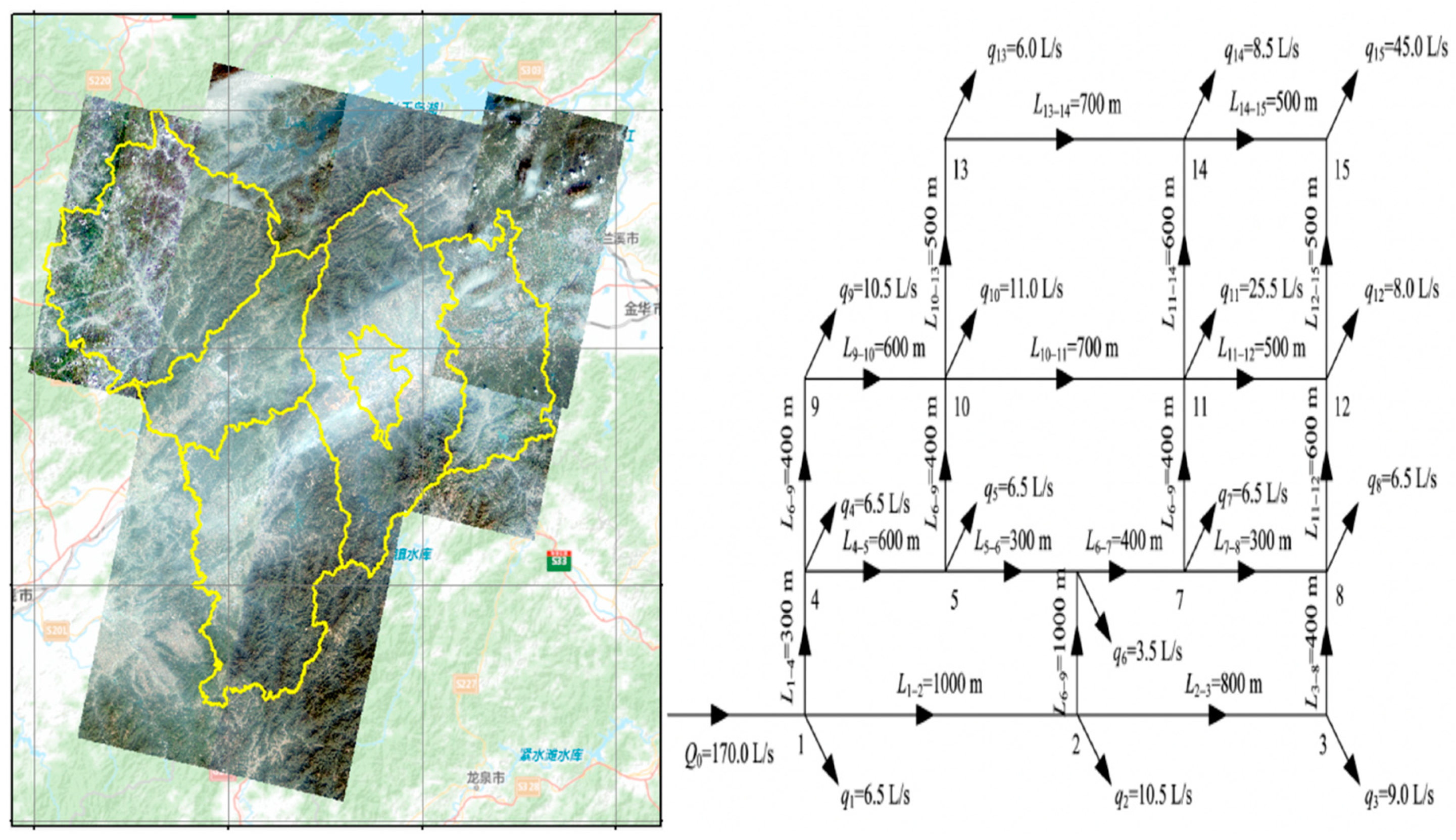
Since the proposed methodology has been shown to be effective for the pipes-only RWSN planning problems, this paper should focus on applying the proposed methodology to deal with the RWSN problems including pumps, valves and pipes in the Jinghua District of Zhejiang Province, China. To provide flexibility, the optimization problem of the water supply network is the multi-variable optimization solved by the MAFSA under multiple loading conditions. The regional water supply network deployment is shown in Figure 4.
An expanded rehabilitation problem is considered where the variables are the tank sizing, tank siting, pipe rehabilitation decisions and pump operation schedules. In order to verify the stability of the algorithm, we set the parameters of MAFSA and run the program 500 times. The optimal solutions has been obtained and the compared results of experiment are shown in Table 4. The cost of the solution includes the capital costs of pipes and tanks as well as the present value of the energy consumed during a specified period. Optimization tends to reduce costs by reducing the diameter of, or completely eliminating, some pipes, thus leaving the system with insufficient capacity to respond to pipe breaks or demands that exceed design values without violating required performance levels. Results show the modified AFSA can effectively and stably search for the optimal solution.
5. Conclusions
The regional water distribution network is a critical infrastructure of urban facilities. Therefore, the planning of the water distribution network must be economical and scientific. This paper researches the multi-objective evolutionary algorithms for planning optimization of a regional water supply network, which formulates the multi-objective model of reliability and economical cost for the regional water supply network according to the hydraulic connectivity. However, the planning of the water supply network is a non-linear and NP-hard optimization problem with many constraining variables. The modified artificial fish swarm algorithm is applied to optimize the planning of the water supply network by dynamic swarm behavior and preying behavior. The experimental results show that the MAFSA can obtain the global optimal solution with high convergence speed compared to other algorithms, which meets the engineering requirement that every demand node in the RWSN is connected to at least one supply source with required flow at adequate pressure.
Author Contributions
Y.L. and M.F. conceived and designed the study; J.Y. and Z.T. performed the experiments; Y.L. and Z.T. wrote the original draft; J.Y. and F.M. reviewed and edited the manuscript. All authors read and approved the manuscript.
Funding
This research was funded by the Natural Science Foundation of Zhejiang Province in China (Grant No. LY18G020009, LQ19G010003), the National Natural Science Foundation of China (Grant No. 71831006, 71804038).
Acknowledgments
This research was supported by the Natural Science Foundation of Zhejiang Province in China and NSFC. We are thankful to our colleagues Xinggang luo and Jiahuan Lu who provided expertise that greatly assisted the research, although they may not agree with all of the interpretations provided in this paper.
Conflicts of Interest
The authors declare no conflicts of interest.
References
- Farmani, R.; Walters, G.; Savic, D. Trade-off between total cost and reliability for any town water distribution network. J. Water Res. Plan. Manag. 2005, 131, 161–171. [Google Scholar] [CrossRef]
- Atilhan, S.; Linke, P.; Abdel-Wahab, A.; El-Halwagi, M. A systems integration approach to the design of regional water desalination and supply networks. Int. J. Process Syst. Eng. 2011, 1, 63–72. [Google Scholar] [CrossRef]
- Shin, H.G.; Park, H. An optimal design of water distribution networks with hydraulic connectivity. J. Water Supply Res. Technol. AQUA 2000, 49, 219–227. [Google Scholar] [CrossRef]
- Wu, Z.Y.; Simpson, A.R. Competent genetic-evolutionary optimization of water distribution systems. J. Comput. Civil Eng. 2001, 15, 89–101. [Google Scholar] [CrossRef]
- Tong, L.; Han, H.; Qiao, J. Design of water distribution network via ant colony optimization. In Proceedings of the 2nd International Conference on Intelligent Control and Information Processing, PART 1, Harbin, China, 25–28 July 2011; pp. 366–370. [Google Scholar]
- Savic, D.; Walters, G.; Randall-Smith, M.; Atkinson, R. Cost savings on large water distribution systems: Design through genetic algorithm optimization. J. Water Res. Plan. Manag. 2000, 18, 256–265. [Google Scholar]
- Vasan, A.; Simonovic, S. Optimization of water distribution network design using differential evolution. J. Water Resour. Plan. Manag. 2010, 136, 279–287. [Google Scholar] [CrossRef]
- Abraham, E.; Stoianov, I. Efficient preconditioned iterative methods for hydraulic simulation of large scale water distribution networks. Procedia Eng. 2015, 119, 623–632. [Google Scholar] [CrossRef]
- Takahashi, S.; Saldarriaga, J.G.; Vega, M.C.; Hernandez, F. Water distribution system model calibration under uncertainty environments. Water Sci. Technol. Water Supply 2010, 10, 31–38. [Google Scholar] [CrossRef]
- Berardi, L.; Ugarelli, R.; Røstum, J.; Giustolisi, O. Assessing mechanical vulnerability in water distribution networks under multiple failures. Water Resour. Res. 2014, 50, 2586–2599. [Google Scholar] [CrossRef]
- Cunha, C.; Sousa, J. Hydraulic infrastructures design using simulated annealing. J. Infrastruct. Syst. 2001, 7, 32–38. [Google Scholar] [CrossRef]
- Tolson, B.A.; Maier, H.R.; Simpson, A.R.; Lence, B.J. Genetic algorithms for reliability-based optimization of water distribution systems. J. Water Resour. Plan. Manag. 2004, 130, 63–72. [Google Scholar] [CrossRef]
- van Dijk, M.; van Vuuren, S.J.; van Zyl, J.E. Optimizing water distribution systems using a weighted penalty in a genetic algorithm. Water Sa 2008, 35, 537–548. [Google Scholar]
- Liu, Y. Improved artificial fish swarm algorithm for vehicle routing problem with backhaul and fuzzy demand. J. Pattern Recognit. Artif. Intell. 2010, 23, 560–564. [Google Scholar]
- Cisty, M. Hybrid Genetic Algorithm and Linear Programming Method for Least-cost Design of Water Distribution Systems. Water Res. Manag. 2010, 24, 1–24. [Google Scholar] [CrossRef]
- Li, L.; Xu, S.; Shi, Z.A. Topological-based method for determination of source-serving districts and drawing pressure-contour in multi-source networks. Water Waste Water Eng. 2001, 27, 5–8. [Google Scholar]
- Walski, T.M. Analysis of water distribution systems; Van Nostrand Reinhold Company: New York, NY, USA, 1984; pp. 284–296. [Google Scholar]
- Di Nardo, A.; Di Natale, M.; Santonastaso, G.F.; Tzatchkov, V.G.; Alcocer-Yamanaka, V.H. Water network sectorization based on graph theory and energy performance indices. J. Water Res. Plan. Manag. 2014, 140, 620–629. [Google Scholar] [CrossRef]
- Keedwell, E.; Khu, S.T. A hybrid genetic algorithm for the design of water distribution networks. Eng. Appl. Artif. Intell. 2005, 18, 461–472. [Google Scholar] [CrossRef]
- Li, M.; Liang, H.B. Application of genetic algorithm in optimal scheduling of water supply system. J. Guangdong Univ. Technol. 2000, 17, 63–65. [Google Scholar]
- Wang, P.; Heng, H.F.; Yue, J. Optimization of urban water network by annealing genetic algorithm. China Water Waste Water 2007, 23, 60–63. [Google Scholar]
Figure 1.
The optimization procedure of the modified artificial fish swarm algorithm (MAFSA).

Figure 2.
The layout of two-loop pipe network.

Figure 3.
The convergent of pipe network by MAFSA.

Figure 4.
The layout of the regional water supply network (https://map.baidu.com).
Figure 4.
The layout of the regional water supply network (https://map.baidu.com).


Table 1.
The pipe cost data of the water distribution network.
| Diameter/mm | Cost ($/m) | Diameter/mm | Cost ($/m) |
|---|---|---|---|
| 50 | 25 | 300 | 250 |
| 75 | 40 | 350 | 300 |
| 100 | 55 | 400 | 450 |
| 150 | 80 | 450 | 650 |
| 200 | 115 | 500 | 850 |
| 250 | 160 | 600 | 1250 |
Table 2.
The node data of the water pipe network.
| Node (Pipe) | Water Flow (L/h) | Ground Elevation (m) |
|---|---|---|
| 1 | 311.12 | 210 |
| 2 | 27.78 | 150 |
| 3 | 27.78 | 160 |
| 4 | 33.33 | 155 |
| 5 | 75.20 | 150 |
| 6 | 91.67 | 165 |
| 7 | 55.56 | 160 |
Table 3.
Compared solutions of different algorithms.
| Node | Solved by MASFA | Solved by GA [19] | |||||
|---|---|---|---|---|---|---|---|
| Diameter/mm | Elevation/m | Free head/kpa | Diameter/mm | Elevation/m | Free head/kpa | ||
| 1 | 450 | 210 | 450 | 210.10 | |||
| 2 | 350 | 202.61 | 515.78 | 350 | 202.71 | 516.56 | |
| 3 | 350 | 195.71 | 350.63 | 350 | 195.87 | 351.53 | |
| 4 | 25 | 196.35 | 419.57 | 50 | 197.90 | 420.42 | |
| 5 | 350 | 191.71 | 401.32 | 350 | 191.12 | 402.98 | |
| 6 | 50 | 193.75 | 299.23 | 75 | 195.20 | 295.96 | |
| 7 | 350 | 190.91 | 295.16 | 350 | 190.18 | 295.77 | |
| 8 | 350 | 350 | |||||
| Cost | 2190,000 | 2215,000 | |||||
Table 4.
The optimization solutions of a regional water supply network by different algorithms.
| Node Pipe | Solved by GA | Solved by MASFA | ||||
|---|---|---|---|---|---|---|
| Length (m) | Diameter (mm) | Water Flow (L/s) | Length (m) | Diameter (mm) | Water Flow (L/s) | |
| 1 | 1000 | 300 | 38.5 | 1 000 | 300 | 36 |
| 2 | 1000 | 200 | 20.5 | 1 000 | 250 | 23 |
| 3 | 300 | 250 | 32.78 | 300 | 250 | 36.8 |
| 4 | 600 | 350 | 53 | 600 | 350 | 57.3 |
| 5 | 300 | 400 | 64.91 | 300 | 400 | 71 |
| 6 | 800 | 200 | 18.72 | 800 | 200 | 16.6 |
| 7 | 400 | 200 | 19.01 | 400 | 150 | 15 |
| 8 | 300 | 150 | 11.92 | 300 | 150 | 12.5 |
| 9 | 400 | 250 | 30.97 | 400 | 300 | 30 |
| 10 | 400 | 200 | 25.64 | 400 | 250 | 18.6 |
| 11 | 600 | 250 | 22.59 | 600 | 200 | 16 |
| 12 | 400 | 300 | 34.78 | 400 | 200 | 12.9 |
| 13 | 400 | 150 | 12.55 | 400 | 250 | 23 |
| 14 | 700 | 200 | 18.6 | 700 | 250 | 23.5 |
| 15 | 600 | 200 | 13.59 | 600 | 200 | 13 |
| Cost ($) | 353800 | 317900 | ||||
© 2019 by the authors. Licensee MDPI, Basel, Switzerland. This article is an open access article distributed under the terms and conditions of the Creative Commons Attribution (CC BY) license (http://creativecommons.org/licenses/by/4.0/).
Share and Cite
MDPI and ACS Style
Liu, Y.; Tao, Z.; Yang, J.; Mao, F. The Modified Artificial Fish Swarm Algorithm for Least-Cost Planning of a Regional Water Supply Network Problem. Sustainability 2019, 11, 4121. https://doi.org/10.3390/su11154121
AMA Style
Liu Y, Tao Z, Yang J, Mao F. The Modified Artificial Fish Swarm Algorithm for Least-Cost Planning of a Regional Water Supply Network Problem. Sustainability. 2019; 11(15):4121. https://doi.org/10.3390/su11154121
Chicago/Turabian StyleLiu, Yi, Zhengpeng Tao, Jie Yang, and Feng Mao. 2019. "The Modified Artificial Fish Swarm Algorithm for Least-Cost Planning of a Regional Water Supply Network Problem" Sustainability 11, no. 15: 4121. https://doi.org/10.3390/su11154121
Note that from the first issue of 2016, this journal uses article numbers instead of page numbers. See further details here.