Improved Salp–Swarm Optimizer and Accurate Forecasting Model for Dynamic Economic Dispatch in Sustainable Power Systems


1
College of Engineering at Wadi Addawaser, Prince Sattam Bin Abdulaziz University, KSA, Al-Kharj 16278, Saudi Arabia
2
Department of Electrical Engineering, Aswan University, Aswan 81542, Egypt
3
Department of Electrical Engineering and Automation, Aalto University, FI-00076 Espoo, Finland
4
Departament d’Enginyeria Informàtica i Matemàtiques, Universitat Rovira i Virgili, 43007 Tarragona, Spain
*
Author to whom correspondence should be addressed.
Sustainability 2020, 12(2), 576; https://doi.org/10.3390/su12020576
Submission received: 16 December 2019
/
Revised: 5 January 2020
/
Accepted: 9 January 2020
/
Published: 12 January 2020
Abstract
:Worldwide, the penetrations of photovoltaic (PV) and energy storage systems are increased in power systems. Due to the intermittent nature of PVs, these sustainable power systems require efficient managing and prediction techniques to ensure economic and secure operations. In this paper, a comprehensive dynamic economic dispatch (DED) framework is proposed that includes fuel-based generators, PV, and energy storage devices in sustainable power systems, considering various profiles of PV (clear and cloudy). The DED model aims at minimizing the total fuel cost of power generation stations while considering various constraints of generation stations, the power system, PV, and energy storage systems. An improved optimization algorithm is proposed to solve the DED optimization problem for a sustainable power system. In particular, a mutation mechanism is combined with a salp–swarm algorithm (SSA) to enhance the exploitation of the search space so that it provides a better population to get the optimal global solution. In addition, we propose a DED handling strategy that involves the use of PV power and load forecasting models based on deep learning techniques. The improved SSA algorithm is validated by ten benchmark problems and applied to the DED optimization problem for a hybrid power system that includes 40 thermal generators and PV and energy storage systems. The experimental results demonstrate the efficiency of the proposed framework with different penetrations of PV.
1. Introduction
Economic dispatch (ED) methods aim to schedule generating units and allocate the demand power among them to determine the best-generating scenarios. ED can benefit power utilities in various ways by systematically minimizing the cost of energy production consistent with the load demand. For this purpose, ED typically increases the usage of the most efficient generators, which can yield lower fuel costs and reduced carbon emissions. A complex mathematical model is solved through multiple computations to satisfy the demand while achieving the minimum generating costs of fuel-based generation stations. These computations are restricted by various constraints of power systems [1,2]. The typical constraints of the ED problem are the capacity of generators, the ramp-rate of generating units, and the power balance.
Conventionally, an approximate quadratic function is employed to mathematically formulate the ED problem in order to reduce the computational complexity. Nevertheless, in practice, the input–output curves of generators have nonlinear characteristic due to the multi-valve steam turbines (so-called valve-point effects). In addition, various faults in the machines prohibit some generators from operating in some zones (i.e., prohibited zones). The existence of the valve-point effects and prohibited zones make the solution space of the ED problem highly nonlinear, and thus increasing the complexity of the optimization process [3].
The static economic dispatch (SED) provides an economical solution to the power of generation stations at a certain load level. Differently, dynamic economic dispatch (DED) optimizes power generation for multiple load levels over a period of time (e.g., one day) [4]. Notably, DED is a more realistic procedure compared with SED because of considering the variation in the demand load and the variation of power generation over the studied period.
After formulating the DED problem mathematically, an optimization method is required to concurrently the fuel cost and carbon emission while handling all constraints. Although the traditional power systems have satisfied the demand loads for a long time, they will not be able to meet the current challenges alone, knowing that the fossil fuel is predicted to run out [5]. The integration of renewable energy sources (RES) into power systems can be attributed to environmental, economic, and social benefits. Driven by these benefits, the future power systems are predicted to be fed by energy sources that are totally renewable. Therefore, modern power systems combine non-conventional resources, such as RES and energy storage systems in order to provide sustainable power systems capable of meeting the significant increase in demand [6,7,8,9,10,11]. For a realistic DED framework and sustainable power systems, there is an essential need to incorporate RES and energy storage systems in the optimization model. The declining trend of the costs of battery energy storage with enhanced efficiency, along with an increasing need to alleviate the intermittent RES generation increased the penetrations of such energy storage systems in the transmission levels. A benefits of the storage systems is to curtail some of the variability challenges related to the RES power, and so smooth the fluctuated generation while providing further charging/discharging control options. Indeed, the DED optimization process can allow the optimal scheduling of the power outputs of generating units and RES according to the load demands over predefined time intervals. Concretely, RES contributes to reducing fuel costs and providing sustainable power and clean energy. Examples of RES are solar energy, wind energy, and tidal energy [12,13,14]. Indeed, solar energy is a necessary form of renewable energy. The earth receives a massive amount of energy from the sun that can be converted into clean electricity directly through photovoltaics (PVs) [15,16] or indirectly through concentrating solar power (CSP) [17]. Although the capital cost of PV farms is high, they are a preferable choice for generating clean electricity [18]. The integration of PV to power systems guarantees efficient power delivery and reduces the amount of CO2 emissions, thus protecting the surrounding environment.
In the last years, several heuristic optimization algorithms have been proposed for solving engineering problems in general due to their high performance and simplicity. These heuristic algorithms are mimicking natural phenomena or the social behaviors of creatures. For instance, particle swarm optimization (PSO) [19], genetic algorithm (GA) [20], ant–lion optimization (ALO) [21], ant colony optimization (ACO) [22], and grey wolf optimization (GWO) [23] are applied to solve the SED problem. The authors of [24] evaluated the performance of moth–flame optimization (MFO), moth swarm algorithm (MSA), GWO, ALO, sine cosine algorithm (SCA), and multi-verse optimization (MVO) with applying mutation operators in solving the SED problem.
Regarding DED, many optimization algorithms have been applied to solve the DED problem, such as symbiotic organisms search (SOS) algorithm, which combines GA, PSO, and SOS in a tri-base population [25]. In [26], the GA algorithm is implemented to optimize the demand side management and the DED as a complementary stage. An accelerated approach is proposed in [27] to solve the DED problem with high computational speed. A hybrid PSO algorithm called BBPSO is presented in [28] for solving the DED problem. In addition, chaotic differential bee colony optimization algorithm (CDBCO) [29], optimality condition decomposition (OCD) technique [30], biogeography-based optimization [31], differential evolution algorithm (DEA) [32,33], and hybrid flower pollination algorithm (HFPA) [34] are implemented to solve the DED problem. Furthermore, hybrid genetic algorithm and bacterial foraging (HGABF) approach [35], weighted probabilistic neural network and biogeography based optimization (WPNN–BBO) [36], multidisciplinary collaborative optimization (MCO) [37], quasi-oppositional group search optimization (QOGSO) [38], and improved real coded genetic algorithm (IRCGA) [39] are also applied to solve the DED problem. In [40], the MILP-IPM approach is applied to solve the DED, and it combines the mixed-integer linear programming (MILP) with the interior point method (IPM).
Indeed, the DED optimization problem is still a challenging issue because of the nonlinear and non-convex characteristics of DED objective functions. The DED optimization process also involves massive calculations to find the optimal values of tens of variables and parameters (high dimensionality) while satisfying the constraints of the power system. The nonlinear, non-convex, and non-differentiable characteristics of the DED, as well as the constraints, may squeeze the solution space. In addition, the intermittent nature of PV increases the difficulty of the DED optimization problem as it adds fluctuations to the power system. These aspects might push the search agents to deviate from the global optima and yield diverse local optima. To cope with these challenges, a robust optimizer is required to provide an accurate solution with low computational complexity.
To cope with the issues above, in this paper, we propose a comprehensive DED framework, deep learning-based forecasting models, and an improved optimizer. Specifically, these major three contributions can be summarized as follows:
- Comprehensive DED framework: A comprehensive DED framework is formulated that includes fuel-based generators, PV, and storage devices in a sustainable power system, considering clear and cloudy profiles of PV.
- Improved optimizer: We propose an improved salp–swarm optimizer that helps manage the global exploration of the DED algorithm and reach reasonable DED solutions. Specifically, we apply a mutation operator to the salp swarm optimizer to increase the exploitation of the search space for improved solutions. The proposed algorithm is validated with ten benchmark problems and then used to optimize the DED problem for a sustainable power system with PV within the studied period.
- Deep learning-based forecasting models: We propose a DED handling strategy that involves the use of PV power and load forecasting models based on deep learning techniques.
2. Comprehensive DED Framework
The main objective of the DED problem is to minimize the costs of the fuel consumed by generator units. This optimization problem is heavily restricted by various practical considerations, e.g., generation constraints of units, ramp-rate constraints of generating units, and power mismatches constraints. Unlike the basic SED problems, DED aims to optimally dispatch the output power of all generators in a number of time instants. Furthermore, we have here considered the PV generation units and energy storage systems, complying with the global policy for establishing sustainable power systems. Figure 1 presents a general structure of sustainable power systems in which renewable energy sources and energy storage systems are interconnected, besides the fuel-based generation stations, to feed various loads.
To address the DED problem, most approaches published in the literature can be itemized into (1) meta-heuristic based optimization methods and (2) conventional optimization-based methods. Examples of meta-heuristic based optimization methods are [25,26,27,28,29,30,31,32,33,34,35,36,37,38,39,40]. Conventional optimization based methods involve: linear programming algorithm [41], lambda iteration method [42], and the interior algorithm [43]. These later methods are usually computationally efficient; however, they are suitable mainly with convex functions [44].
The optimal dispatch can be achieved through maximizing the total fuel-cost savings (TFS) of the fuel-based generator units, or in other words minimizing the total fuel-cost (TFC). During time intervals , the corresponding demand power at these occasions must be optimally allocated among the generating units. The TFC is proportional to the number of thermal generators, and TFS can be formulated as follows:
in which
where is the total fuel cost of all generator units to supply without PV and energy storage systems, and is the total fuel cost of all generator units to supply () with PV and energy storage systems. , , , and are, respectively, the total predicted load power, available active power generation of PV based on the predicted environmental conditions (i.e., solar radiation), active power curtailment of PV, and the charging/discharging power of the energy storage systems at time instant . For generator , , , and are its cost coefficients, and , and are the coefficients of valve-point effects, n is the number of thermal generators to be scheduled, t represents the current time, T is the total time of the studied period, and is the thermal power generated from the generator at time t. The valve-point effect can be considered as a practical operation constraint of thermal generators. This effect introduces a ripple in the heat rate function, yielding a discontinuous nonlinear fuel cost function that has multiple local minima. In Equation (2), a second order quadratic cost function is formulated with a rectified sinusoidal term for precise modeling of the cost function of generators considering the valve-point effect.
The DED is mathematically formulated as:
The equality and inequality constraints of the power system, PV, and energy storage systems are listed below:
- Equality constraints
- Inequality constraints
Constraint (4) represents the balance between the active powers of all thermal generators, the PV system, and the energy storage systems with respect to the total load demand and active power losses in the power system at each time instant t. is the output power from the PV unit at time t expressed by Label (5), and are the charging and discharging power of the storage device at time t, respectively, is the total demand power at time t, and represents the transmission losses computed by Label (6) in which represents B-coefficients.
Constraints (7), (8), and (9) represent the upper and lower operational boundaries, the ramp-up limit, and the ramp-down limit of each thermal generator at each time instant t, respectively. and are the minimum and maximum limits of the output power from the thermal generator, respectively. and represent the ramp-up and ramp-down boundaries of the thermal generator, respectively.
Constraints (10) can set the maximum allowed curtailed power of PV according to the regulations of utilities. is a factor where its value ranges from 0 to 1. In this work, this latter factor is set to zero to prevent the active power curtailment. Regarding the energy storage device, it has two operational constraints represented by (11) and (12). and are the minimum and maximum charging rate limits of the storage energy devices, respectively. and are the minimum and maximum state of charge limits of the storage energy devices, respectively. Note that the decision variables in the DED optimization problem are: the output power from each thermal generator , curtailed active PV power , charging rate of the storage energy devices , and state of charge of the storage energy devices for all time instants during the dispatching period, which is the next day in this work.
Besides the consideration of valve point effects, the prohibited operating zones of generators can model their persistent physical operation boundaries (e.g., generator faults, excessive vibrations, turbine constraints). Therefore, the feasible zones for the ith generator can be mathematically formulated as follows:
where z is the number of the prohibited operating zones for the generator. and represent the lower and upper (MW) power boundaries of prohibited operating zone for the generator, respectively. Figure 2 illustrates the basic generator costs curve, the costs considering valve point effect, and the impacts of the prohibited operating zones on the two curves. Figure 2 implies that, if a generator has z prohibited zones, its operating region will be split into isolated feasible sub-regions, yielding multiple decision spaces for the DED problem. As noticed, by considering both valve-point effects and the prohibited operating zones of generators, the optimization model became more complex and non-convex, and so required robust optimization algorithms to be accurately solved.
The output power of a PV module depends on the ambient temperature and solar irradiation. It can be modeled as follows [45,46]:
where is the cell temperature and is the ambient temperature at time t, refers to the nominal operating cell temperature, R is the solar irradiation, is the short circuit current, is the temperature coefficient of current, is the temperature of the standard test conditions, is the open-circuit voltage, is the temperature coefficient of voltage, is the fill factor, is the number of cells in the module, and and are the voltage and current at the maximum power point, respectively. In this paper, one hour resolution of the data and the dispatch cycle have been considered. However, the proposed model is general, and can be applied to other resolutions.
3. Proposed DED Algorithm
The step-by-step procedure for the proposed method can be summarized as follows:
- Step 1: Read system data, including cost coefficients of generation stations, power limits of generation stations, ramp rate limits for each generation station, and B-loss coefficients. Read the historical datasets of load and PV solar radiation, and data of energy storage systems.
- Step 2: Set the population of the improved SSA algorithm, number of agents, and the maximum number of iterations.
- Step 3: Forecast the PV radiation and load for the period in which the system is required to be optimally dispatched.
- Step 4: Run the improved SSA algorithm considering the mutation operator and the handling strategy of the various constraints.
- Step 5: Save and print the calculated results, including the scheduling of the generation stations, and energy storage systems, and the total costs.
3.1. Improved Salp–Swarm Algorithm (ISSA)
Swarm intelligence algorithms are widely used for solving complex optimization problems. Salp swarm algorithm (SSA) is a bio-inspired optimization algorithm where it mimics the swarming behavior of salps that belong to the family Salpidae [47]. Salps have a transparent body and look like jellyfishes, and they have a similar movement behavior in water. Salps almost form swarms called salp chains in deep oceans. The salp chain population consists of leaders and followers; the leader is the first salp in the swarm, where it tracks the food source and guides the remainder of the swarm followers. The position of all salps are saved in a two-dimensional matrix labeled S. The SSA algorithm assumes that there is a food source called in the search space as the swarm target. The positions of salps can be represented as:
where n is the number of salps, and m is the number of variables. The leader’s position is updated according to the following formula:
where, in the dimension, is the 1st salp, while represents the food source, and are the upper and lower boundaries, respectively. X2 and X3 dictate if the next position in jth dimension should be towards positive infinity or negative infinity as well as the step size.
In SSA, is responsible for balancing exploration and exploitation. It can be calculated as follows:
In this equation, l represents the current iteration, and L represents the total number of iterations, , and are random numbers uniformly generated in the interval [0,1]. They control the step size and the next position in the dimension.
The position of the followers is updated according to Newton’s law of motion as follows:
where , is the salp in the dimension, t is time, is the initial velocity, and where . Since the time in the optimization problem represents iteration, the discrepancy between iterations equals and assuming Equation (22) can be reformulated as follows:
where is the salp in the dimension.
The SSA optimization method can be trapped into local minima, which can lead to inaccurate results, especially with non-convex complex optimization problems, such as DED. To precisely solve the DED problem, we improve the performance of SSA by adopting a mutation operator. The improved SSA with the mutation operator is able to improve the convergence ability of the basic SSA algorithm by adjusting the searching direction in space in an adaptive way. Specifically, the mutation operator utilized in this paper is expressed as follows:
where , , are the best three positions in the current population (i.e., the positions that have the top fitness values), , and is the fitness value.
3.2. Satisfying Various Constraints
When employing the improved SSA algorithm employed for solving the DED model, many updated solutions may be infeasible, especially in the early stage of the optimizer. To solve this issue, we utilize a reforming algorithm to enforce the updated solutions to be within their allowed limits, i.e., getting into the feasible search space. Consider as an updated set of all candidate solutions, and it is formulated as:
where , , and represent, respectively, the set of power values of thermal generators, PV, and energy storage systems at all time periods . First, the reforming algorithm enforces all variables with respected to their upper and lower boundaries for the variables at first time instant, i.e., t = 1. For instance, the upper and lower boundaries (, ) for the generator at time period t can be formulated as follows:
Similar formulations are considered to enforce the control variables of PV and storage energy systems with respect to their upper and lower boundaries for the variables at first time instant (). Then, for each time intervals , all the feasible search space of the upper and the lower boundaries at are explored. If the corresponding variables violate the explored feasible search space boundaries, their values are corrected to these upper/lower boundaries; otherwise, their values are kept the same.
3.3. Forecasting Models
Indeed, PV power forecasting is complex due to the fluctuating profiles of the weather (e.g., solar irradiance and temperature). Recurrent neural networks have been used in many applications, such as the optimal PV planning (i.e., determining the optimal sizes of PV plants with considering their intermittent generation), the optimal scheduling of thermal generators considering the predicted values of the PV generation for reducing operational costs of the grid, and the optimal management of PV plants while mitigating the operational problems, such as voltage violations and reverse power flow. Specifically, a deep long-short term memory (LSTM) recurrent neural network has been employed in the literature to forecast the intermittent PV power [48,49,50] and solar irradiance [51,52,53]. The merit of the LSTM is that it can model the temporal changes in the data due to their recurrent architecture and memory units. Unlike the traditional recurrent neural networks, LSTMs were designed to avoid the long-term dependency problem. LSTM can capture abstract concepts in the time-series forecasting problems.
Here, a DED handling strategy is introduced that involves the use of solar radiation (R) and load forecasting models. To build a solar radiation forecasting model, we propose the use of LSTM. Here, solar radiation forecasting is formulated as a regression problem. To train the solar radiation forecasting models, year-long solar radiation datasets with time resolution 1 h are used. The solar radiation dataset is restructured as follows: input and target. The input is the solar radiation at time steps , and the target is the solar radiation at time step , where is the width of the lag window. The load dataset is restructured in the same way.
Figure 3 shows the block diagram of LSTM, where it receives an input sequence in which the activation units are used to trigger the gates. Each LSTM block has a cell with a state at time step t. The input gate , forget gate , and output gate are used to manage the reading or updating processes of this cell. The LSTM operation is expressed as follows:
where W are weights of the LSTM model that can be learned in the training stage. In this paper, we adopt our LSTM model proposed in [48] to construct a solar radiation forecasting model and load forecasting model, separately. The two LSTM models have a visible layer with one input, a hidden layer with four LSTM blocks, and an output layer that gives the target (solar radiation or load). The sigmoid activation function is used. The LSTM models are trained with the mean-squared error loss function, ADAM optimizer, and 100 epochs with a batch size of 1.
We use an adaptive moment estimation (ADAM) optimizer, a method for efficient stochastic optimization that only requires first-order gradients with little memory requirements. ADAM computes separate learning rates for each weight from estimates of first and second moments of the gradients as well as an exponentially decaying average of previous gradients. It is memory efficient since it does not keep a history of anything (just the rolling averages). We use an ADAM optimizer because it is computationally efficient (small memory requirements), has straightforward implementation, invariant to diagonally rescale the gradients, and suitable for optimizing the problems that are large in terms of data and for solving problems with dense noisy (or sparse gradients). The hyper-parameters of ADAM need little tuning. ADAM is also suitable for non-stationary objectives, which is the case of solar radiation forecasting.
4. Results and Discussion
To verify the effectiveness of the proposed method, we evaluate it using ten benchmark problems [47] (see Table 1) and the DED problem. In this study, we simulate a sustainable power system containing 40 thermal generators, PV, and energy storage systems. We provide the data of thermal generators in Table 2. We compare the results of the improved SSA (ISSA) with other optimization algorithms: SSA, MFO [54], and MVO [55]. The main inspiration for MFO is the navigation method of moths. In short, moths fly at night by keeping a fixed angle concerning the moon. The MFO mathematically models the navigation behaviour of moths to perform optimization. In turn, the main inspiration for the MVO algorithm relies on some concepts in cosmology: (1) white hole, (2) black hole, and (3) wormhole. The mathematical models of these concepts are implemented to perform optimization. It is a fact that there is no meta-heuristic best suited for treating all optimization models, complying with the No Free Lunch (NFL) theorem [56]. Therefore, we can conclude that each method of the three algorithms (SSA, MFO and MVO) gives a supervisor performance for specified types of functions, not all of them. In this work, we have developed an improved version of SSA to specifically solve the DED model. The parameters of the ISSA optimizer are set as follows: the population size is 30, the dimension is 10, and the maximum iterations number is 1000. All experiments have been carried out in MATLAB 2019a.
4.1. Analyzing the Performance of ISSA with Ten Benchmark Problems
The proposed method is implemented on ten benchmark problems, which are shown in Table 1. These problems have a challenging search space similar to the real complex search space. Indeed, they can verify the performance of algorithms and check their balancing strategy between the exploration and the exploitation phases. In Table 3, we show the average (Ave) and standard deviation (Std) values of the fitness function for 10 runs. The dimension of F1 is 30, the dimension of F2, F3, F4, F5, F6, F7, F8, and F9 is 30, and the dimension of F10 is 100. As shown, ISSA achieves results better than SSA with the benchmark problems (F1, F5, F7, and F9) in terms of Ave and Std, thanks to the mutation operator. Furthermore, ISSA outperforms MFO and MVO for the ten functions. In the case of F10, which is a highly nonlinear with a dimension of 100. With such complex optimization problem, ISSA achieves an Ave and Std values of 6.3844 and 1.3105, respectively. In turn, SSA and MVO achieves higher Ave values. MFO gives the worst Ave value (19.849) compared to the other optimizer. Driven by this superior performance, the proposed ISSA can be applied for the large scale optimization problems with several variables and wide search space, such as the DED problem. Note that the computational time of these methods is within 5 s.
4.2. Analyzing the Performance of an LSTM Forecasting Model
To evaluate the performance of the proposed method, two yearly PV datasets (dataset1 and dataset2) are used in this paper. We divide each dataset into training and testing datasets. A total of 70% of the samples are used to train the forecasting model, while the remaining samples are used for testing the model. We used the root mean square error (RMSE) to evaluate the performance of the forecasting models. RMSE can be defined as follows:
In this equation, and are the ith predicted and actual values, respectively, and N is the size of the testing dataset.
The performance of the LSTM forecasting method is compared with four PV forecasting methods: multiple linear regression (MLR), bagged regression trees (BRT), and ANN methods. These methods have been widely used in the literature for forecasting PV generation [58]. Thus, we used them in this paper to demonstrate the effectiveness of the LSTM model. As we can see in Table 4, LSTM gives small RMSE values with dataset1 and dataset2 (82.15 and 136.87). MLR and BRT give the highest RMSE values. With dataset1, the RMSE values of MLR and BRT are 384.90 and 494.46, respectively, while they are 329.11 and 416.212 with dataset2, respectively. Indeed, MLR and BRT were developed for stationary time series forecasting and thus they are not suitable for forecasting solar radiation. In the case of ANN, we have tried different configurations such as using one or two layers while changing the number of neurons from 1 to 50 with a step of 1. We found that the ANN model gives its best results with two layers and seven neurons. The RMSE values of ANN are 377.072 and 348.931 with dataset1 and dataset2, respectively. The forecasting RMSE values of LSTM are lower than MLR, BRT, and ANN methods. Indeed, MLR, BRT, and ANN methods do not have memory units, and thus they cannot handle the fluctuations in solar radiation. However, the architecture of the ANN method is a similar to LSTM, but it does not contain memory units or a recurrent architecture. In turn, LSTM uses the information learned in the previous time steps to estimate the current value, leading to accurate forecasting results.
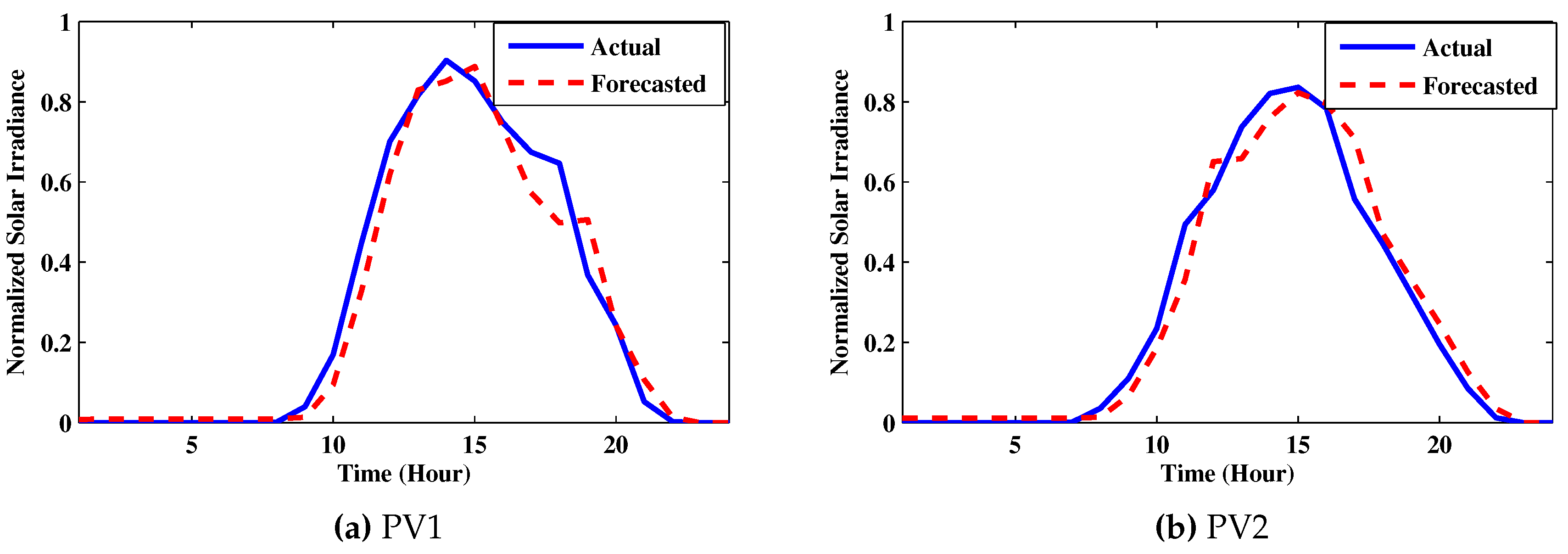
Figure 4 shows the predicted solar irradiance for one day using the LSTM model for the dataset1 and dataset2. As shown, the LSTM can accurately predict the solar irradiance for the two datasets where the actual and predicted values are highly correlated. Notably, this high accuracy will have pronounced positive impacts on the DED problem since the decision variables will be properly computed considering accurate forecasting results. In this study, we demonstrate the effectiveness of deep learning approaches against traditional machine learning algorithms. Therefore, our recommendation is to utilize deep machine learning to accurately forecast PV power. In our paper, we utilize deep LSTM as an example, but other deep methods can give similar accuracy rates, but we do not investigate other deep learning, which is left as a future work.
4.3. Analyzing the Performance of ISSA with the DED Problem
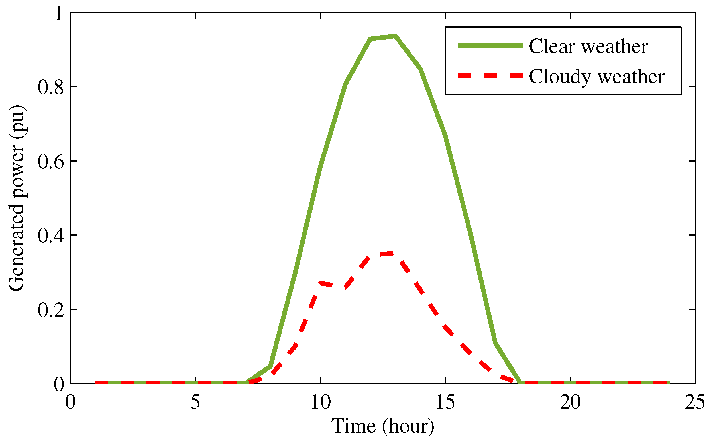
Here, we simulate a sustainable power system containing 40 thermal generators, PV, and energy storage systems. The studied period is 24 h in which PV and load profiles are predicted using LSTM. The demand power is shown in Figure 5, and the output power of PV is shown in Figure 6 during clear and cloudy days. Below, we present two test cases of the proposed method with different weather conditions (clear and cloudy days). The capacity of the energy storage system (Sodium Sulfur Battery system) is 128 MWh. The parameters of the energy storage system are assumed as follows [59]: = 50%, and = 100%. The maximum allowed curtailed power () is set to zero.
Case 1: the performance of the proposed method with clear weather.Table 5 demonstrates the effectiveness of the proposed algorithm to minimize the total fuel costs with 0, 10, 20, 30, 40, and 50% penetrations of PV concerning the load. As we can see in this table, ISSA gives the lowest fuel cost for the six PV penetrations compared to SSA, MFO, and MVO. With ISSA, the fuel cost at 0% penetration of PV (i.e., without PV) is 2.7687*106 $ while it drops to 2.4228*106 $ at 50% penetration. It is worth noting that higher penetration levels of the PV can lead to reduced fuel costs. In the case of cloudy weather, it is expected that the output power of thermal generation units and energy storage devices will compensate the decrease of the PV power to satisfy the load, and so the fuel cost will be increased. Note that, if some clouds exist on a particular day, they will not affect the accuracy of the LSTM prediction model since the model is trained using a data of one year containing different weather conditions (clear, rainy, overcast, and cloudy).
Indeed, with higher penetrations of PV, the power generated from the thermal generators is less than the ones with lower penetrations. This power is optimally allocated among the thermal generators by ISSA through various generating scenarios over the studied period. Figure 7 shows the generated power of the 40 thermal generators over 24 h (see color bar) at the PV penetration of 50%. The x-axis of this figure represents the 40 generations (1, 2, …, 40) where the corresponding generated power values are shown. Each color on the color map represents the optimal generated power of the 40 thermal generators at each time interval (1, 2, …, 24). Note that each layer has a different color and a width. The color represents the time instance while the width represents the MW generated power of each generator. The width of each layer indicates the boundaries of the generated power of each generator, which can be easily tracked in this figure. For instance, the widths of layers corresponding to generators from 1 to 5 are narrow compared with generators from 15 to 20. This figure can quantify the daily generation of the different generators. For example, we can notice that generator number 20 has a very high production profile compared with generator 10. This can help the system operators to specify the generators that will be expected to be heavily loaded among the other generators according to the forecasting PV and load profiles as well as the solved DED problem.
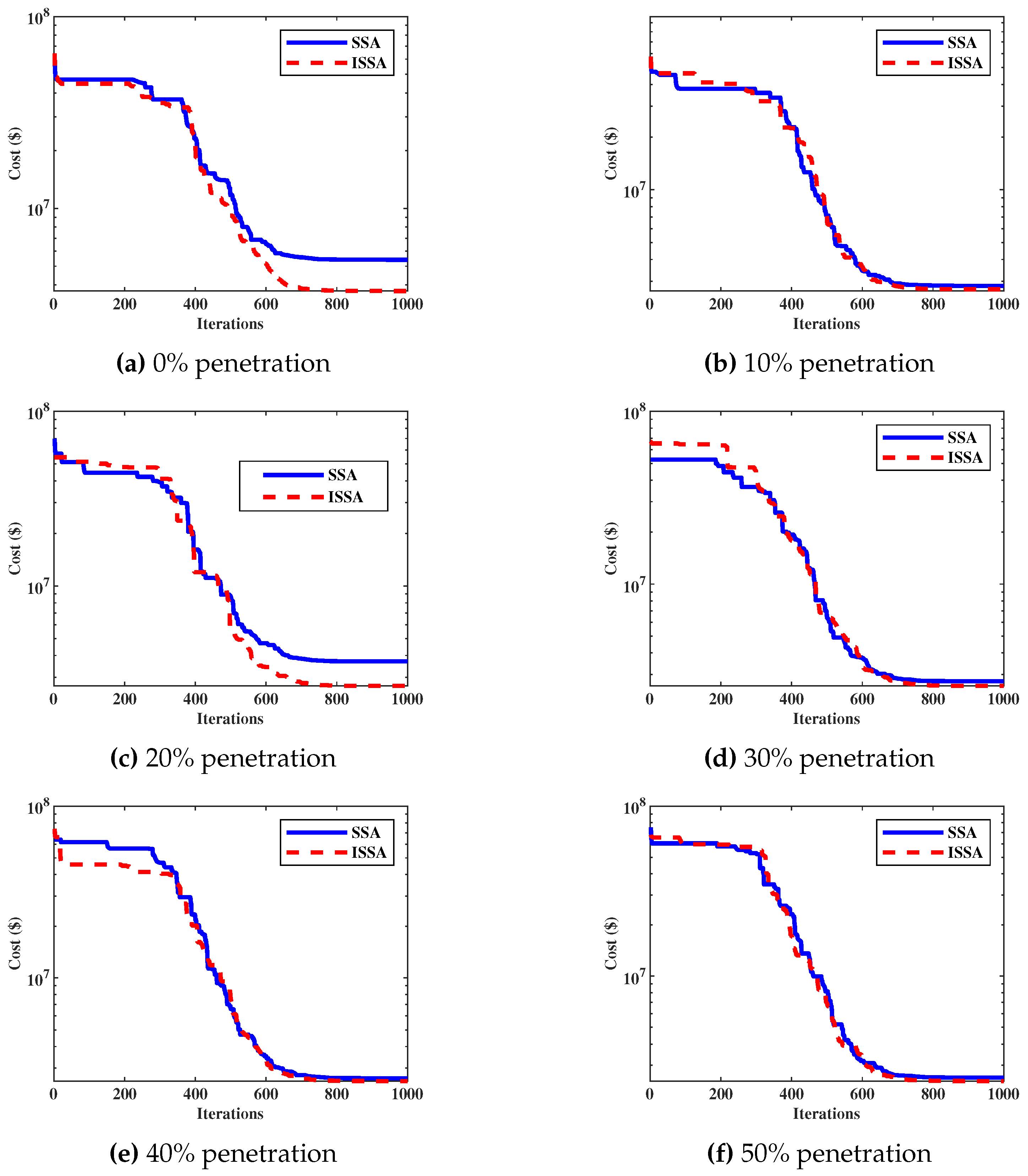
Figure 8 shows the charging and discharging of the storage device for the different penetration cases. The ISSA algorithm can optimally schedule both the thermal generators and energy storage systems simultaneously to minimize the fuel cost. Figure 9 shows the convergence characteristics of ISSA. As we can see, the ISSA algorithm achieves better convergence characteristics, especially at 0%, 20%, and 30% penetration levels of the PV, where it converges rapidly compared to SSA.
Case 2: the performance of the proposed method with cloudy weather. In the case of cloudy weather, the output power of PV (Figure 6) is less than that of the clear weather as the output PV generation mainly depends on the solar irradiation. Therefore, the required powers from the thermal generators are increased causing higher fuel costs compared to case 1 (clear weather). Figure 10 shows the allocated load demand among the 40 thermal generators. Similar to Figure 7, the color map shows that the generators are within their operating boundaries (represented by layer width). It is clear that the scheduling of the 40 thermal generators with the cloudy weather profile is far different compared to the scheduling of the clear weather. Figure 11 shows the charging and the discharging of the storage device. Importantly, we notice higher storage rates with higher PV penetrations. Table 6 shows a comparison between the resulted fuel cost using ISSA, SSA, MFO, and MVO during cloudy days. Similar to the results of case 1 (clear day), ISSA achieves the lowest fuel cost. Figure 12 shows the convergence characteristics of ISSA, SSA, MFO, and MVO, in which ISSA has a stable and faster convergence. The improvement in performance when applying ISSA (with the mutation operator) is more significant in the case of 20%, 30%, and 50% PV penetrations than the other levels.
In this work, the optimization process is solved once, not repeated for each hour. This process aims to schedule the operations of generators day ahead considering daily forecast PV and load profiles. Therefore, the optimizer will be run offline (i.e., computational speed is not a vital factor), and where the computed optimal scheduling will be applied in the next day. However, the computational time of the optimizer when solving the DED is less than 10 min. These simulations reveal the effectiveness of the proposed algorithm to solve the DED problem with intermittent PV and energy storage systems. This analysis demonstrates that the proposed DED model can guarantee a minimum operational cost (total fuel costs) for sustainable power systems.
5. Conclusions and Future Work
Sustainable power systems provide the solution for satisfying the increased demand while reducing the harmful impacts of fuel-based generation stations. In this paper, a comprehensive DED framework has been proposed considering various profiles of PV (clear and cloudy) and energy storage systems. The DED model aims at minimizing the total fuel cost of power generation stations while considering various constraints of generation stations, PV, and energy storage systems. An improved optimization algorithm has been proposed to solve this optimization model. In particular, a mutation mechanism has been combined with SSA to produce to enhance the exploitation of the search space so that it provides a better population to get the optimal global solution. In addition, we have proposed a DED handling strategy that involves the use of PV power and load forecasting models based on deep learning models. The proposed algorithm has been validated with ten benchmark problems and then applied to the DED problem. A power system of forty thermal generators and PV is simulated considering the storage device with various PV penetrations (0%, 10%, 20%, 30%, 40%, and 50%). Two test cases have been analyzed: clear and cloudy weather conditions. ISSA obtains accurate results compared to three other optimization algorithms (SSA, MFO, and MVO). In future work, the proposed comprehensive DED model will be integrated with other sustainable energy resources (e.g., hydro energy, wind energy).
Author Contributions
Conceptualization, K.M. and M.A.-N.; methodology, K.M., E.M., and M.A.-N.; software, M.A.-N.; validation; formal analysis, K.M., E.M., and M.A.-N.; investigation, K.M., M.A.-N., and Z.M.A.; resources, K.M., M.A.-N., and Z.M.A.; data curation, E.M.; writing—original draft preparation, K.M., E.M., and M.A.-N.; writing—review and editing, K.M., M.A.-N., and Z.M.A.; visualization; supervision, K.M., M.A.-N. and Z.M.A.; project administration, K.M., M.A.-N., and Z.M.A. All authors have read and agreed to the published version of the manuscript.
Funding
This research received no external funding.
Conflicts of Interest
The authors declare no conflict of interest.
References
- Yang, S.; Tan, S.; Xu, J.X. Consensus based approach for economic dispatch problem in a smart grid. IEEE Trans. Power Syst. 2013, 28, 4416–4426. [Google Scholar] [CrossRef]
- Abujarad, S.Y.; Mustafa, M.; Jamian, J. Recent approaches of unit commitment in the presence of intermittent renewable energy resources: A review. Renew. Sustain. Energy Rev. 2017, 70, 215–223. [Google Scholar] [CrossRef]
- Lee, F.N.; Breipohl, A.M. Reserve constrained economic dispatch with prohibited operating zones. IEEE Trans. Power Syst. 1993, 8, 246–254. [Google Scholar] [CrossRef]
- Zaman, M.; Elsayed, S.M.; Ray, T.; Sarker, R.A. Evolutionary algorithms for dynamic economic dispatch problems. IEEE Trans. Power Syst. 2015, 31, 1486–1495. [Google Scholar] [CrossRef]
- Rahman, M.M.; Mostafiz, S.B.; Paatero, J.V.; Lahdelma, R. Extension of energy crops on surplus agricultural lands: A potentially viable option in developing countries while fossil fuel reserves are diminishing. Renew. Sustain. Energy Rev. 2014, 29, 108–119. [Google Scholar] [CrossRef] [Green Version]
- Abas, N.; Kalair, A.; Khan, N. Review of fossil fuels and future energy technologies. Futures 2015, 69, 31–49. [Google Scholar] [CrossRef]
- Mohamed, A.A.A.; Ali, S.; Alkhalaf, S.; Senjyu, T.; Hemeida, A.M. Optimal Allocation of Hybrid Renewable Energy System by Multi-Objective Water Cycle Algorithm. Sustainability 2019, 11, 6550. [Google Scholar] [CrossRef] [Green Version]
- Alkhalaf, S.; Senjyu, T.; Saleh, A.A.; Hemeida, A.M.; Mohamed, A.A.A. A MODA and MODE Comparison for Optimal Allocation of Distributed Generations with Different Load Levels. Sustainability 2019, 11, 5323. [Google Scholar] [CrossRef] [Green Version]
- Ahmed, E.M.; Aly, M.; Elmelegi, A.; Alharbi, A.G.; Ali, Z.M. Multifunctional Distributed MPPT Controller for 3P4W Grid-Connected PV Systems in Distribution Network with Unbalanced Loads. Energies 2019, 12, 4799. [Google Scholar] [CrossRef] [Green Version]
- Abdel-Nasser, M.; Mahmoud, K.; Kashef, H. A Novel Smart Grid State Estimation Method Based on Neural Networks. IJIMAI 2018, 5, 92–100. [Google Scholar] [CrossRef] [Green Version]
- Mahmoud, K.; Hussein, M.M.; Abdel-Nasser, M.; Lehtonen, M. Optimal Voltage Control in Distribution Systems With Intermittent PV Using Multiobjective Grey-Wolf-Lévy Optimizer. IEEE Syst. J. 2019, 1–11. [Google Scholar] [CrossRef] [Green Version]
- Clancy, J.; Gaffney, F.; Deane, J.; Curtis, J.; Gallachóir, B.Ó. Fossil fuel and CO2 emissions savings on a high renewable electricity system–a single year case study for Ireland. Energy Policy 2015, 83, 151–164. [Google Scholar] [CrossRef]
- Mohamed, F.; AbdelNasser, M.; Mahmoud, K.; Kamel, S. Accurate economic dispatch solution using hybrid whale-wolf optimization method. In Proceedings of the 2017 Nineteenth International Middle East Power Systems Conference (MEPCON), Cairo, Egypt, 19–21 December 2017; pp. 922–927. [Google Scholar]
- Mahmoud, K.; Abdel-Nasser, M. Efficient SPF approach based on regression and correction models for active distribution systems. IET Renew. Power Gener. 2017, 11, 1778–1784. [Google Scholar] [CrossRef]
- Novakovic, B.; Nasiri, A. 1-Introduction to electrical energy systems. In Electric Renewable Energy Systems; Rashid, M.H., Ed.; Academic Press: Boston, MA, USA, 2016; pp. 1–20. [Google Scholar] [CrossRef]
- Mahmoud, K.; Abdel-Nasser, M. Fast-yet-Accurate Energy Loss Assessment Approach for Analyzing/Sizing PV in Distribution Systems using Machine Learning. IEEE Trans. Sustain. Energy 2018, 1025–1033. [Google Scholar] [CrossRef]
- Cirocco, L.R.; Belusko, M.; Bruno, F.; Boland, J.; Pudney, P. Maximising revenue via optimal control of a concentrating solar thermal power plant with limited storage capacity. IET Renew. Power Gener. 2016, 10, 729–734. [Google Scholar] [CrossRef]
- Shaahid, S.M. Economic feasibility of decentralized hybrid photovoltaic-diesel technology in saudi arabia. Therm. Sci. 2017, 21, 745–756. [Google Scholar] [CrossRef] [Green Version]
- Mahor, A.; Prasad, V.; Rangnekar, S. Economic dispatch using particle swarm optimization: A review. Renew. Sustain. Energy Rev. 2009, 13, 2134–2141. [Google Scholar] [CrossRef]
- Rastgoufard, S.; Iqbal, S.; Hoque, M.T.; Charalampidis, D. Genetic algorithm variant based effective solutions for economic dispatch problems. In Proceedings of the 2018 IEEE Texas Power and Energy Conference (TPEC), College Station, TX, USA, 8–9 February 2018; pp. 1–6. [Google Scholar]
- Kamboj, V.K.; Bath, S.; Dhillon, J. Solution of non-convex economic load dispatch problem using Grey Wolf Optimizer. Neural Comput. Appl. 2016, 27, 1301–1316. [Google Scholar] [CrossRef]
- Pothiya, S.; Ngamroo, I.; Kongprawechnon, W. Ant colony optimisation for economic dispatch problem with non-smooth cost functions. Int. J. Electr. Power Energy Syst. 2010, 32, 478–487. [Google Scholar] [CrossRef]
- Jayabarathi, T.; Raghunathan, T.; Adarsh, B.; Suganthan, P.N. Economic dispatch using hybrid grey wolf optimizer. Energy 2016, 111, 630–641. [Google Scholar] [CrossRef]
- Mostafa, E.; Abdel-Nasser, M.; Mahmoud, K. Performance evaluation of metaheuristic optimization methods with mutation operators for combined economic and emission dispatch. In Proceedings of the 2017 Nineteenth International Middle East Power Systems Conference (MEPCON), Cairo, Egypt, 19–21 December 2017; pp. 1004–1009. [Google Scholar]
- Duman, S. Symbiotic organisms search algorithm for optimal power flow problem based on valve-point effect and prohibited zones. Neural Comput. Appl. 2017, 28, 3571–3585. [Google Scholar]
- Mellouk, L.; Boulmalf, M.; Aaroud, A.; Zine-Dine, K.; Benhaddou, D. Genetic Algorithm to Solve Demand Side Management and Economic Dispatch Problem. Procedia Comput. Sci. 2018, 130, 611–618. [Google Scholar] [CrossRef]
- Chen, G.; Li, C.; Dong, Z. Parallel and distributed computation for dynamical economic dispatch. IEEE Trans. Smart Grid 2016, 8, 1026–1027. [Google Scholar] [CrossRef]
- Zhang, Y.; Gong, D.W.; Geng, N.; Sun, X.Y. Hybrid bare-bones PSO for dynamic economic dispatch with valve-point effects. Appl. Soft Comput. 2014, 18, 248–260. [Google Scholar] [CrossRef]
- Lu, P.; Zhou, J.; Zhang, H.; Zhang, R.; Wang, C. Chaotic differential bee colony optimization algorithm for dynamic economic dispatch problem with valve-point effects. Int. J. Electr. Power Energy Syst. 2014, 62, 130–143. [Google Scholar] [CrossRef]
- Rabiee, A.; Mohammadi-Ivatloo, B.; Moradi-Dalvand, M. Fast dynamic economic power dispatch problems solution via optimality condition decomposition. IEEE Trans. Power Syst. 2013, 29, 982–983. [Google Scholar] [CrossRef]
- Ma, H.; Yang, Z.; You, P.; Fei, M. Multi-objective biogeography-based optimization for dynamic economic emission load dispatch considering plug-in electric vehicles charging. Energy 2017, 135, 101–111. [Google Scholar] [CrossRef]
- Jebaraj, L.; Venkatesan, C.; Soubache, I.; Rajan, C.C.A. Application of differential evolution algorithm in static and dynamic economic or emission dispatch problem: A review. Renew. Sustain. Energy Rev. 2017, 77, 1206–1220. [Google Scholar] [CrossRef]
- Hongfeng, Z. Dynamic economic dispatch based on improved differential evolution algorithm. Clust. Comput. 2018, 1–8. [Google Scholar] [CrossRef]
- Dubey, H.M.; Pandit, M.; Panigrahi, B. Hybrid flower pollination algorithm with time-varying fuzzy selection mechanism for wind integrated multi-objective dynamic economic dispatch. Renew. Energy 2015, 83, 188–202. [Google Scholar] [CrossRef]
- Elattar, E.E. A hybrid genetic algorithm and bacterial foraging approach for dynamic economic dispatch problem. Int. J. Electr. Power Energy Syst. 2015, 69, 18–26. [Google Scholar] [CrossRef]
- Nanjundappan, D. Hybrid weighted probabilistic neural network and biogeography based optimization for dynamic economic dispatch of integrated multiple-fuel and wind power plants. Int. J. Electr. Power Energy Syst. 2016, 77, 385–394. [Google Scholar]
- Xie, M.; Luo, W.; Cheng, P.; Ke, S.; Ji, X.; Liu, M. Multidisciplinary collaborative optimisation-based scenarios decoupling dynamic economic dispatch with wind power. IET Renew. Power Gener. 2018, 12, 727–734. [Google Scholar] [CrossRef]
- Basu, M. Quasi-oppositional group search optimization for multi-area dynamic economic dispatch. Int. J. Electr. Power Energy Syst. 2016, 78, 356–367. [Google Scholar] [CrossRef]
- Pattanaik, J.K.; Basu, M.; Dash, D.P. Improved real coded genetic algorithm for dynamic economic dispatch. J. Electr. Syst. Inf. Technol. 2018, 5, 349–362. [Google Scholar] [CrossRef]
- Pan, S.; Jian, J.; Yang, L. A hybrid MILP and IPM approach for dynamic economic dispatch with valve-point effects. Int. J. Electr. Power Energy Syst. 2018, 97, 290–298. [Google Scholar] [CrossRef] [Green Version]
- Somuah, C.; Khunaizi, N. Application of linear programming redispatch technique to dynamic generation allocation. IEEE Trans. Power Syst. 1990, 5, 20–26. [Google Scholar] [CrossRef]
- Lin, C.E.; Viviani, G. Hierarchical economic dispatch for piecewise quadratic cost functions. IEEE Trans. Power Appar. Syst. 1984, 1170–1175. [Google Scholar] [CrossRef]
- Irisarri, G.; Kimball, L.; Clements, K.; Bagchi, A.; Davis, P. Economic dispatch with network and ramping constraints via interior point methods. IEEE Trans. Power Syst. 1998, 13, 236–242. [Google Scholar] [CrossRef]
- Binetti, G.; Davoudi, A.; Naso, D.; Turchiano, B.; Lewis, F.L. A distributed auction-based algorithm for the nonconvex economic dispatch problem. IEEE Trans. Ind. Inform. 2013, 10, 1124–1132. [Google Scholar] [CrossRef]
- Atwa, Y.; El-Saadany, E.; Salama, M.; Seethapathy, R. Optimal renewable resources mix for distribution system energy loss minimization. IEEE Trans. Power Syst. 2009, 25, 360–370. [Google Scholar] [CrossRef]
- Ali, A.; Raisz, D.; Mahmoud, K.; Lehtonen, M. Optimal placement and sizing of uncertain PVs considering stochastic nature of PEVs. IEEE Trans. Sustain. Energy 2019. [Google Scholar] [CrossRef] [Green Version]
- Mirjalili, S.; Gandomi, A.H.; Mirjalili, S.Z.; Saremi, S.; Faris, H.; Mirjalili, S.M. Salp Swarm Algorithm: A bio-inspired optimizer for engineering design problems. Adv. Eng. Softw. 2017, 114, 163–191. [Google Scholar] [CrossRef]
- Abdel-Nasser, M.; Mahmoud, K. Accurate photovoltaic power forecasting models using deep LSTM-RNN. Neural Comput. Appl. 2019, 31, 1–14. [Google Scholar] [CrossRef]
- Kim, S.G.; Jung, J.Y.; Sim, M.K. A Two-Step Approach to Solar Power Generation Prediction Based on Weather Data Using Machine Learning. Sustainability 2019, 11, 1501. [Google Scholar] [CrossRef] [Green Version]
- Li, G.; Wang, H.; Zhang, S.; Xin, J.; Liu, H. Recurrent neural networks based photovoltaic power forecasting approach. Energies 2019, 12, 2538. [Google Scholar] [CrossRef] [Green Version]
- Yu, Y.; Cao, J.; Zhu, J. An LSTM Short-Term Solar Irradiance Forecasting Under Complicated Weather Conditions. IEEE Access 2019, 7, 145651–145666. [Google Scholar] [CrossRef]
- Jeon, B.K.; Lee, K.H.; Kim, E.J. Development of a Prediction Model of Solar Irradiances Using LSTM for Use in Building Predictive Control. J. Korean Sol. Energy Soc. 2019, 39, 41–52. [Google Scholar]
- Husein, M.; Chung, I.Y. Day-Ahead Solar Irradiance Forecasting for Microgrids Using a Long Short-Term Memory Recurrent Neural Network: A Deep Learning Approach. Energies 2019, 12, 1856. [Google Scholar] [CrossRef] [Green Version]
- Mirjalili, S. Moth-flame optimization algorithm: A novel nature-inspired heuristic paradigm. Knowl.-Based Syst. 2015, 89, 228–249. [Google Scholar] [CrossRef]
- Mirjalili, S.; Mirjalili, S.M.; Hatamlou, A. Multi-verse optimizer: A nature-inspired algorithm for global optimization. Neural Comput. Appl. 2016, 27, 495–513. [Google Scholar] [CrossRef]
- Wolpert, D.H.; Macready, W.G. No Free Lunch Theorems for Optimization. IEEE Trans. Evol. Comput. 1997, 1, 67. [Google Scholar] [CrossRef] [Green Version]
- Güvenç, U.; Sönmez, Y.; Duman, S.; Yörükeren, N. Combined economic and emission dispatch solution using gravitational search algorithm. Sci. Iran. 2012, 19, 1754–1762. [Google Scholar] [CrossRef] [Green Version]
- Sharifzadeh, M.; Sikinioti-Lock, A.; Shah, N. Machine-learning methods for integrated renewable power generation: A comparative study of artificial neural networks, support vector regression, and Gaussian Process Regression. Renew. Sustain. Energy Rev. 2019, 108, 513–538. [Google Scholar] [CrossRef]
- You, S.; Rasmussen, C.N. Generic modelling framework for economic analysis of battery systems. In Proceedings of the IET Renewable Power Generation Conference, Edinburgh, UK, 6–8 September 2011. [Google Scholar]
Figure 1.
An overview of the structure of sustainable power systems.

Figure 2.
Structure of sustainable power systems.

Figure 3.
The block diagram of LSTM.

Figure 4.
The predicted solar irradiance using LSTM for one day.

Figure 5.
Demand load during the day.

Figure 6.
PV output power during clear and cloudy days.

Figure 7.
Generated power of the 40 thermal generators with case 1 at 50% penetration.

Figure 8.
Charging and discharging of storage device with clear weather.

Figure 9.
Convergence characteristics of the ISSA with case 1.

Figure 10.
Generated power of the 40 thermal generators with case 2 at 50% penetration.

Figure 11.
Charging and discharging of storage device with cloudy weather.

Figure 12.
Convergence characteristics of the ISSA with case 2.


Table 1.
The benchmark problems.
| Function | Dimension | Limits | |
|---|---|---|---|
| 30 | [−100,100] | 0 | |
| 10 | [−10,10] | 0 | |
| 10 | [−100,100] | 0 | |
| 10 | [−100,100] | 0 | |
| 10 | [−30,30] | 0 | |
| 10 | [−100,100] | 0 | |
| 10 | [−1.28,1.28] | 0 | |
| 10 | [−500,500] | 0 | |
| 10 | [−5.12,5.12] | 0 | |
| 100 | [−32,32] | 0 |
Table 2.
Characteristics of the 40 thermal generators [57].
Table 2.
Characteristics of the 40 thermal generators [57].
| Unit | Cost Coefficients | Power Limits | |||||
|---|---|---|---|---|---|---|---|
| a ($/MW2 h) | b ($/MWh) | c ($/h) | e ($/h) | f (rad/MW) | Pmin (MW) | Pmax (MW) | |
| 1 | 0.00690 | 6.73 | 94.705 | 100 | 0.084 | 36 | 114 |
| 2 | 0.00690 | 6.73 | 94.705 | 100 | 0.084 | 36 | 114 |
| 3 | 0.02028 | 7.07 | 309.540 | 100 | 0.084 | 60 | 120 |
| 4 | 0.00942 | 8.18 | 369.030 | 150 | 0.063 | 80 | 190 |
| 5 | 0.01140 | 5.35 | 148.890 | 120 | 0.077 | 47 | 97 |
| 6 | 0.01142 | 8.05 | 222.330 | 100 | 0.084 | 68 | 140 |
| 7 | 0.00357 | 8.03 | 287.710 | 200 | 0.042 | 110 | 300 |
| 8 | 0.00492 | 6.99 | 391.980 | 200 | 0.042 | 135 | 300 |
| 9 | 0.00573 | 6.60 | 455.760 | 200 | 0.042 | 135 | 300 |
| 10 | 0.00605 | 12.9 | 722.820 | 200 | 0.042 | 130 | 300 |
| 11 | 0.00515 | 12.9 | 635.200 | 200 | 0.042 | 94 | 375 |
| 12 | 0.00569 | 12.8 | 654.690 | 200 | 0.042 | 94 | 375 |
| 13 | 0.00421 | 12.5 | 913.400 | 300 | 0.035 | 125 | 500 |
| 14 | 0.00752 | 8.84 | 1760.400 | 300 | 0.035 | 125 | 500 |
| 15 | 0.00752 | 8.84 | 1760.400 | 300 | 0.035 | 125 | 500 |
| 16 | 0.00752 | 8.84 | 1760.400 | 300 | 0.035 | 125 | 500 |
| 17 | 0.00313 | 7.97 | 647.850 | 300 | 0.035 | 220 | 500 |
| 18 | 0.00313 | 7.95 | 647.850 | 300 | 0.035 | 220 | 500 |
| 19 | 0.00313 | 7.97 | 647.850 | 300 | 0.035 | 242 | 550 |
| 20 | 0.00313 | 7.97 | 647.850 | 300 | 0.035 | 242 | 550 |
| 21 | 0.00298 | 6.63 | 785.960 | 300 | 0.035 | 254 | 550 |
| 22 | 0.00298 | 6.63 | 785.960 | 300 | 0.035 | 254 | 550 |
| 23 | 0.00284 | 6.66 | 794.530 | 300 | 0.035 | 254 | 550 |
| 24 | 0.00284 | 6.66 | 794.530 | 300 | 0.035 | 254 | 550 |
| 25 | 0.00277 | 7.10 | 801.320 | 300 | 0.035 | 254 | 550 |
| 26 | 0.00277 | 7.10 | 801.320 | 300 | 0.035 | 254 | 550 |
| 27 | 0.52124 | 3.33 | 1055.100 | 120 | 0.077 | 10 | 150 |
| 28 | 0.52124 | 3.33 | 1055.100 | 120 | 0.077 | 10 | 150 |
| 29 | 0.52124 | 3.33 | 1055.100 | 120 | 0.077 | 10 | 150 |
| 30 | 0.01140 | 5.35 | 148.890 | 120 | 0.077 | 47 | 97 |
| 31 | 0.00160 | 6.43 | 222.920 | 150 | 0.063 | 60 | 190 |
| 32 | 0.00160 | 6.43 | 222.920 | 150 | 0.063 | 60 | 190 |
| 33 | 0.00160 | 6.43 | 222.920 | 150 | 0.063 | 60 | 190 |
| 34 | 0.00010 | 8.95 | 107.870 | 200 | 0.042 | 90 | 200 |
| 35 | 0.00010 | 8.62 | 116.580 | 200 | 0.042 | 90 | 200 |
| 36 | 0.00010 | 8.62 | 116.580 | 200 | 0.042 | 90 | 200 |
| 37 | 0.01610 | 5.88 | 307.450 | 80 | 0.098 | 25 | 110 |
| 38 | 0.01610 | 5.88 | 307.450 | 80 | 0.098 | 25 | 110 |
| 39 | 0.01610 | 5.88 | 307.450 | 80 | 0.098 | 25 | 110 |
| 40 | 0.00313 | 7.97 | 647.830 | 300 | 0.035 | 242 | 550 |
Table 3.
Comparing the performance of the ISSA, SSA, MFO, and MVO with ten benchmark problems.
| Function | Optimization Method | |||||||
|---|---|---|---|---|---|---|---|---|
| ISSA | SSA | MFO | MVO | |||||
| Ave | Std | Ave | Std | Ave | Std | Ave | Std | |
| F1 | 0.00000 | 0.00000 | 0.00001 | 0.00000 | 0.00014 | 0.00017 | 1.1969 | 0.1407 |
| F2 | 0.00001 | 0.00000 | 0.00000 | 0.00000 | 0.00000 | 0.00000 | 0.0357 | 0.0128 |
| F3 | 0.00000 | 0.00000 | 0.0000 | 0.0000 | 0.00000 | 0.00001 | 0.1152 | 0.0771 |
| F4 | 0.00002 | 0.00000 | 0.00002 | 0.00000 | 0.6032 | 1.3682 | 0.0927 | 0.035 |
| F5 | 4.16500 | 3.1621 | 7.2112 | 2.4367 | 8.1502 | 7.7184 | 88.0909 | 125.6254 |
| F6 | 0.00000 | 0.00000 | 0.0000 | 0.0000 | 0.00000 | 0.00000 | 0.0156 | 0.0043 |
| F7 | 0.00130 | 0.0014 | 0.0048 | 0.00300 | 0.00490 | 0.00260 | 0.0035 | 0.0018 |
| F8 | −2955.8 | 184.4003 | −2746.9 | 239.6771 | −3305.9 | 243.2327 | −3006 | 337.0665 |
| F9 | 0.29850 | 0.6715 | 14.9244 | 4.5474 | 17.4118 | 6.7359 | 14.6334 | 4.7858 |
| F10 | 6.3844 | 1.3105 | 7.4999 | 1.5513 | 19.8439 | 0.2259 | 7.1737 | 6.7536 |
Table 4.
Comparison with related methods.
| Method | MLR | BRT | ANN | LSTM |
|---|---|---|---|---|
| RMSE of dataset1 | 384.8951 | 494.4633 | 377.072 | 82.15 |
| RMSE of dataset2 | 329.11 | 416.212 | 348.931 | 136.87 |
| Recurrent? | × | × | × | √ |
| Can it remember? | × | × | × | √ |
Table 5.
Total fuel cost for case 1 (clear weather).
| Penetration | Fuel Cost*106 ($) | |||
|---|---|---|---|---|
| ISSA | SSA | MFO | MVO | |
| 0% | 2.7687 | 2.8451 | 3.0904 | 2.8945 |
| 10% | 2.7017 | 2.8162 | 2.9153 | 2.8945 |
| 20% | 2.6790 | 2.7783 | 2.8518 | 2.8945 |
| 30% | 2.5714 | 2.7385 | 2.7949 | 2.7446 |
| 40% | 2.5155 | 2.6131 | 2.7614 | 2.7446 |
| 50% | 2.4228 | 2.5395 | 2.5892 | 2.7446 |
Table 6.
Total fuel cost for case 2 (cloudy weather).
| Penetration | Fuel Cost*106 ($) | |||
|---|---|---|---|---|
| ISSA | SSA | MFO | MVO | |
| 0% | 2.7687 | 2.8451 | 3.0904 | 2.8945 |
| 10% | 2.7261 | 2.8298 | 2.8824 | 2.8824 |
| 20% | 2.6849 | 2.7861 | 2.7945 | 2.7945 |
| 30% | 2.6710 | 2.7861 | 2.7823 | 2.7823 |
| 40% | 2.5244 | 2.6905 | 2.7171 | 2.7171 |
| 50% | 2.4877 | 2.6495 | 2.6641 | 2.6641 |
© 2020 by the authors. Licensee MDPI, Basel, Switzerland. This article is an open access article distributed under the terms and conditions of the Creative Commons Attribution (CC BY) license (http://creativecommons.org/licenses/by/4.0/).
Share and Cite
MDPI and ACS Style
Mahmoud, K.; Abdel-Nasser, M.; Mustafa, E.; M. Ali, Z. Improved Salp–Swarm Optimizer and Accurate Forecasting Model for Dynamic Economic Dispatch in Sustainable Power Systems. Sustainability 2020, 12, 576. https://doi.org/10.3390/su12020576
AMA Style
Mahmoud K, Abdel-Nasser M, Mustafa E, M. Ali Z. Improved Salp–Swarm Optimizer and Accurate Forecasting Model for Dynamic Economic Dispatch in Sustainable Power Systems. Sustainability. 2020; 12(2):576. https://doi.org/10.3390/su12020576
Chicago/Turabian StyleMahmoud, Karar, Mohamed Abdel-Nasser, Eman Mustafa, and Ziad M. Ali. 2020. "Improved Salp–Swarm Optimizer and Accurate Forecasting Model for Dynamic Economic Dispatch in Sustainable Power Systems" Sustainability 12, no. 2: 576. https://doi.org/10.3390/su12020576
Note that from the first issue of 2016, this journal uses article numbers instead of page numbers. See further details here.