Freeway Short-Term Travel Speed Prediction Based on Data Collection Time-Horizons: A Fast Forest Quantile Regression Approach


1
College of Metropolitan Transportation, Beijing University of Technology, Beijing 100124, China
2
College of Artificial Intelligence and Automation, Beijing University of Technology, Beijing 100124, China
3
Department of Civil Engineering, King Fahd University of Petroleum & Minerals (KFUPM), Dhahran 31261, Saudi Arabia
4
Department of Artificial Intelligence and Management, Group Gema-Esi Business School/IA School, 61 bis rue des Peupliers, Boulogne-Billancourt, 92100 Paris, France
*
Author to whom correspondence should be addressed.
Sustainability 2020, 12(2), 646; https://doi.org/10.3390/su12020646
Submission received: 11 December 2019
/
Revised: 9 January 2020
/
Accepted: 10 January 2020
/
Published: 16 January 2020
(This article belongs to the Special Issue Road Traffic Engineering and Sustainable Transportation)
Abstract
:Short-term traffic speed prediction is vital for proactive traffic control, and is one of the integral components of an intelligent transportation system (ITS). Accurate prediction of short-term travel speed has numerous applications for traffic monitoring, route planning, as well as helping to relieve traffic congestion. Previous studies have attempted to approach this problem using statistical and conventional artificial intelligence (AI) methods without accounting for influence of data collection time-horizons. However, statistical methods have received widespread criticism concerning prediction accuracy performance, while traditional AI approaches have too shallow architecture to capture non-linear stochastics variations in traffic flow. Hence, this study aims to explore prediction of short-term traffic speed at multiple time-ahead intervals using data collected from loop detectors. A fast forest quantile regression (FFQR) via hyperparameters optimization was introduced for predicting short-term traffic speed prediction. FFQR is an ensemble machine learning model that combines several regression trees to improve speed prediction accuracy. The accuracy of short-term traffic speed prediction was compared using the FFQR model at different data collection time-horizons. Prediction results demonstrated the adequacy and robustness of the proposed approach under different scenarios. It was concluded that prediction performance of FFQR was significantly enhanced and robust, particularly at time intervals larger than 5 min. The findings also revealed that speed prediction error (in terms of quantiles loss) ranged between 0.58 and 1.18.
1. Introduction
With rapid growth in car ownership, traffic congestion has become one of the most critical social concerns in urban metropolitans around the world. In addition to restraining smooth inter-city mobility, it also poses a threat to the urban economy and stable development [1,2,3,4]. Traffic congestion could be recurrent resulting from routine cyclic fluctuations in traffic, or it may be non-recurrent due to emergency incidents, special events, unforeseen bad weather conditions, and so forth. China is one of the fastest growing economies in the world, second after the US. China’s transport sector has witnessed a dramatic increase during the past four decades, with the motorization rate exponentially accumulated from 1.8 million in 1980 to 340 million in 2019 [5,6]. Similarly, motor vehicle ownership in the country has increased from 1.8 per 1000 persons in 1980 to 179 in 2019 [6]. China has also become the largest car market with annual sales exceeding 24 million vehicles in 2016 [7]. But this rapid economic development has also brought severe consequences in terms of energy, environment, and social costs. According to statistics, the most prominent cities in the country are accounting for huge daily economic loss worth $1 billion, due to traffic congestion [8], which is an alarming situation. Further, traffic congestion has slowed down the average running speed in many Chinese cities. For example, in 2011, the average driving speed in Beijing was 7.5 miles per hour compared to 12.4 in Hong Kong, 15.5 in New York city, and 18 in London despite the fact, that all of these cities have car populations larger than Beijing [9]. Additionally, around 30% of Beijing’s air pollution is dominated by transport emissions [9]. Thus, it is essential to identify the underlying causes, and properly tackle the issue of traffic congestion.
Accurate traffic information is of great importance for managing traffic congestion in urban areas. In addition to information about existing traffic conditions, accurate knowledge about traffic state parameters (traffic flow, density, speed) in subsequent short time intervals is vital for deciding on a potential control and management strategy. Accurate traffic prediction is an integral component of advanced travelers information system (AITS) in intelligent transportation system (ITS). It has numerous applications such as route planning, navigation, dynamic traffic assignment, congestion estimation, and other mobility services [10,11]. Among traffic state parameters, travel speed is one of the main indexes that reflect the quality of operating conditions along the highways. Travel speed directly influences the implementation of traffic management strategies like traffic control system (TCS) and traffic guidance System (TGS) [12]. The accuracy of travel speed prediction is largely influenced by available data, traditionally from loop detectors, radars, and traffic cameras fixed at some important road locations. However, with the increasing amount of available data collected from mobile services (smartphones and on-board GPS devices), probe vehicles, remote traffic microwave sensors (RTMS), and various internet of things (IOT) sensors, the challenge is no longer related to data quantity, but rather to extraction and modeling of useful information from this data [13]. With accurate travel speed prediction, travelers can make more informed decisions about trip generation and dynamic route planning. Developing traffic congestion can be mitigated collectively, and traffic conditions can become more stable. However, it is always challenging to realistically estimate short-term future travel speed conditions because of the complexity of road network, instability and stochasticity in traffic flow, and floating vehicles speed.
In previous literature, different approaches have been utilized for short-term travel speed prediction including time series analysis methods [14,15], statistical regressions [16], artificial neural (NN) [17,18], and support vector regression (SVR) methods [19]. Although, time series and statistical methods have good theoretical interpretations, these methods have been frequently questioned regarding prediction performance. While traditional machine learning methods like NN and SVR have too shallow architecture to capture latent interactions among variables, particular for complex network. Recently, with unprecedented opportunities for collecting detailed data, deep learning has drawn widespread research attention due to its excellent ability to extract essential data features, with enhanced computational efficiency at a rapid pace. Although prediction accuracy from all machine learning is relatively better, it receives criticism of being operated within a black box lacking sound theoretical basis. Regarding travel speed prediction, most of the methods used in the existing literature have focused on selecting arbitrary time-horizons for data collection without accounting for influence of different time intervals on predictive performance. It is essential to study the influence of varying time-horizons for the collection of data on travel speed prediction. Present study attempts to fill this research gap using a novel regression approach.
Given the variability in travel speed under recurrent and non-recurrent traffic conditions, the objective of current research study is to make better speed predictions under multiple traffic data collection time-horizons, that would ultimately assist in alleviating congestion in the city of Beijing. Speed data with varying time intervals was collected from loop detectors on 2nd Ring Road in Beijing. The specific contributions of this study are: (i) short-term traffic speed performance using novel FFQR approach, to the best of our knowledge, FFQR has not been used in traffic flow forecasting; (ii) to compare the performance of proposed approach under varying data collection time-horizons (i.e., 5, 10, and 15 min intervals); (iii) to conduct hyperparameter optimization of model by random grid to improve the prediction accuracy; (iv) to demonstrate prediction accuracy for varying data collection time-horizons in terms of quantile loss. Study results indicated that the proposed approach was efficient and robust under the considered multiple time-horizons.
The remainder of this paper is structured as below. Section 2 provides a detailed review of existing literature in traffic flow forecasting in general, and particularly short-term speed prediction. Section 3 describes the study area, data used in the study, and key algorithm parameters setting. Section 4 discusses the architecture of the proposed approach in context of current study, and model performance evaluation. Section 5 presents results and discussions with reference to quantile loss associated with multiple time-ahead scenarios. Finally, Section 6 summarizes the key study conclusions, study limitations, and recommendations for potential future work.
2. Related Work
2.1. Literature Review
Travel speed is an essential measure for estimating the quality of operating conditions in traffic networks. Accurate short-term travel speed prediction plays a vital role in proactive traffic control in ITS. Short-term traffic prediction involves precise predictions of various traffic parameters such as traffic flow, speed, density, and occupancy [20,21]. Researchers are challenged continuously by the consequences of rapid urbanization, including severe congestion and safety issues. The ideal conditions for precise prediction of traffic state is that vehicles occupy their respective lane without frequent lane change maneuvers, as sudden lane changes have been found to be associated with low prediction accuracy as well as motor vehicle crashes [22,23]. Uncertainty in travel time and speed estimation can be disastrous, leading to extreme man-hours wasted waiting in a queue, increased fuel consumption, and vehicular emissions [24,25,26]. Travel speed prediction refers to the estimation of average vehicle fleet speed in the near future (for example, 1 to 60 min) using real-time traffic data. Robust and accurate traffic state prediction has numerous applications for active traffic management, intelligent driving, high-precision navigation, route planning, and several other advanced applications [18,27]. However, realistic traffic state prediction is a challenging task due to the non-linear and stochastic nature of traffic data. Also, it is challenging to record individual vehicle speed on a busy urban route, particularly during rush hours. This issue was addressed by Anil et al., who proposed a comprehensive framework incorporating a processing module with traffic cameras [28]. The proposed architecture was found capable of tracking and estimating speed in real-time for every single vehicle in the camera frame. Further, most of the existing approaches for traffic state prediction rely on previous speed records, and it is closely associated with other different traffic variables such as density and traffic volume on contagious links and road segments. These roads may not be necessarily linked to the target road, but changes in traffic attributes of surrounding roads will affect travel speed later on [29]. However, considering too many irrelevant adjacent roads are likely to aggravate the complexity of the prediction algorithm as well as decreasing its running performance, while considering only a few adjacent links will degrade its prediction accuracy. Hence, a sensitivity analysis is recommended to select the most relevant adjacent roads providing a reasonable trade-off between the two.
Traffic state prediction always requires prior real-time speed information/data from devices such as loop detectors, traffic cameras, GPS navigation devices, and mobile phones. It is rather difficult and impractical to capture network-wide speed data using fixed location devices; GPS and mobile phones may serve as a suitable alternative. Mobile phone navigation devices have several advantages over the former methods such as high accuracy, reliability, optimal performance in real-time, less construction time and costs, etc. [30]. To detect the instantaneous speed of vehicles, remote traffic microwave sensor (RTMS) is another useful non-intrusive new piece of equipment. The device is installed roadside and is capable of directly recording moving or stationary vehicle speed without interrupting traffic flow. In addition to capturing speed data, RTMS can provide reliable information about traffic volume, density, and occupancy for multiple lanes simultaneously, even during adverse weather conditions [31,32]. In recent years, researchers have proposed various methods to improve the accuracy of speed estimation. For example, speed estimation results from the cellular probe system, and loop detectors were aggregated using the travel-time based method [33]. To avoid tracking each vehicle using any labeled data, velocity-based estimation approach was proposed [34]. A recent study introduced a path inference approach [35], using taxi GPS traces having low sampling frequency to accurately estimate network-wide speed on congested links.
The principal input parameters in predicting short-term travel speed are traffic flow, travel speed, and occupancy. While each of the three parameters for traffic congestion can be used, both speed and traffic flow correlate with occupancy. Furthermore, speed is more directly associated with traffic operation status. A study previously conducted found that short-term speed prediction results are significantly influenced by real-time dynamic traffic control [36]. Traffic speed is a commonly used metric to evaluate the road segment’s traffic status. A wide variety of sensors, including GPS vehicles, inductive loop detectors, and mobile phones, have been continuously collecting large scale traffic data promoting the advancement of data-driven intelligent transport systems (ITS). In general, the term “short-term” relates to a prediction horizon of up to one hour. It predicts traffic conditions ahead of the present moment for a few seconds to a few hours, which is the optimal time for individual navigation and global urban traffic planning. Existing traffic state prediction methods with traffic sensor data are commonly divided into three categories: data-driven, model-driven, and data-driven streaming [37]. In recent years the analysis of road traffic data and future traffic characteristics were investigated by statistical, machine learning, and data mining techniques. Numerous methodologies have been introduced and adopted for short-term traffic prediction, and the ultimate objective remains the same: to acquire the prediction results accurately and as efficiently as possible. Predicting with machine learning models, a fine setting of parameters for any model has a significant impact on its performance, as highlighted by previous study [38].
2.2. Previous Studies
During the past two decades, numerous studies have been conducted for travel speed prediction. Researchers have considered various methods based on statistical modelling, neural networks, machine learning, big data, etc. These methods are studied under two main categories i.e., parametric and non-parametric based. Recently, some studies have utilized hybrid-based techniques combining two or more methods to enhance prediction accuracy. Parametric methods have a fixed structure, where parameters are learned using an observed data set [39]. Parametric methods have explicit theoretical interpretations, and are easily implemented. These methods require high data quality, with a data sequence desired to be stable and accurate. However, the nature of obtained traffic data is usually unstable and stochastic, which limits their use in complex applications. Some parametric methods explored for short-term traffic flow and speed prediction are: time series models [40,41]; exponential smoothing model [42]; spectral analysis [43,44]; autoregressive integrated moving average (ARIMA) models [45,46,47]; ARIMA model with extended structures like Kohonen-ARIMA [48]; model seasonal autoregressive integrated moving average (SARIMA) model [49]; and ARIMA with Kalman filter [50]. Like parametric methods, non-parametric methods assess dynamic correlation directly from training data; however, they have an enhanced adaptive learning ability and strong generalization resulting in better prediction accuracy [51]. Some nonparametric used for speed prediction are: artificial neural network (ANN) model [52,53]; multi-type neural network [54]; deep convolutional neural network [55]; kernel smoothing [56], k-nearest neighbor approach [57,58]; and support vector regression model (SVRM) [59,60]. Ma et al. suggested a long short-term memory neural network commonly known as LSTM-NN, using a remote sensor network data in the city of Beijing [32]. In another study, researchers compared LSTM with a convolutional neural-network (CNN) for network-wide travel speed prediction, and found that CNN was more robust than LSTM with a 42.91% improvement in mean square error [55].
Recently some studies have focused on hybrid approaches in an attempt to improve prediction accuracy considering the merits and application associated with each prediction method. Few studies that have utilized hybrid models are; the Bayesian-neural network approach [61]; hybrid fuzzy rule-based approach [62]; state-space approach coupled with least-squares support vector machine (LS-SVM) [63]; KNN-Gaussian regression process [64]; and chaos-wavelet analysis support vector machine approach (CWSVM) [65]. Intuitively, hybrid models provide better prediction accuracy compared to single prediction models [66,67,68]. However, complex model architecture and high computational efforts limit their network-wide implementation [43]. With the advent of big data and machine learning technology, different types of machine learning are being explored in short-term travel speed prediction. Some commonly used machine learning models utilized for travel speed prediction are: evolving fuzzy neural network (EFNN) [69]; long short-term memory networks (LSTM) [32,70]; bi-directional long short- term memory neural-network (Bi LSTM-NN) [71]; and include support vector regression (SVR) [59]. NN, and fuzzy schemes have also been successfully used in other related disciplines such as image retrieval, feature extraction, and signal cycle length optimization [72,73,74].
It is evident from the reviewed literature, that different approaches have been adopted for traffic state prediction to improve prediction accuracy. These may be categorized into three distinct categories, parametric, non-parametric methods, and methods based on deep learning. The former has reliable theoretical interpretations but is not considered good in terms of prediction accuracy because of the stochastic nature of traffic data, while the non-parametric methods works in a black box with a weak theoretical basis. However, machine learning approaches are relatively flexible, with very little or no initial assumptions for input parameters. Machine learning methods have much deeper and complex architecture to capture stochastic variation thus yielding improved prediction accuracy. Further these methods are capable of processing outliers, missing, and noisy data. Comprehensive review of existing literature also indicates that most of the studies focused on selecting arbitrary time-horizons for data collection without taking into account the effects of time interval on predictive performance. It is important to study the influence of varying time-horizons for the data collection on travel speed prediction. Hence, this paper examines short-term travel speed performance of novel fast random forest quantile regression (FRFQ) using varying data collection time-horizons speed data from four loop detectors on a freeway segment of 2nd Ring Road in Beijing. To the best of our knowledge, this method has not been used in previous studies for traffic forecasting.
3. Data Collection and Parameters Settings
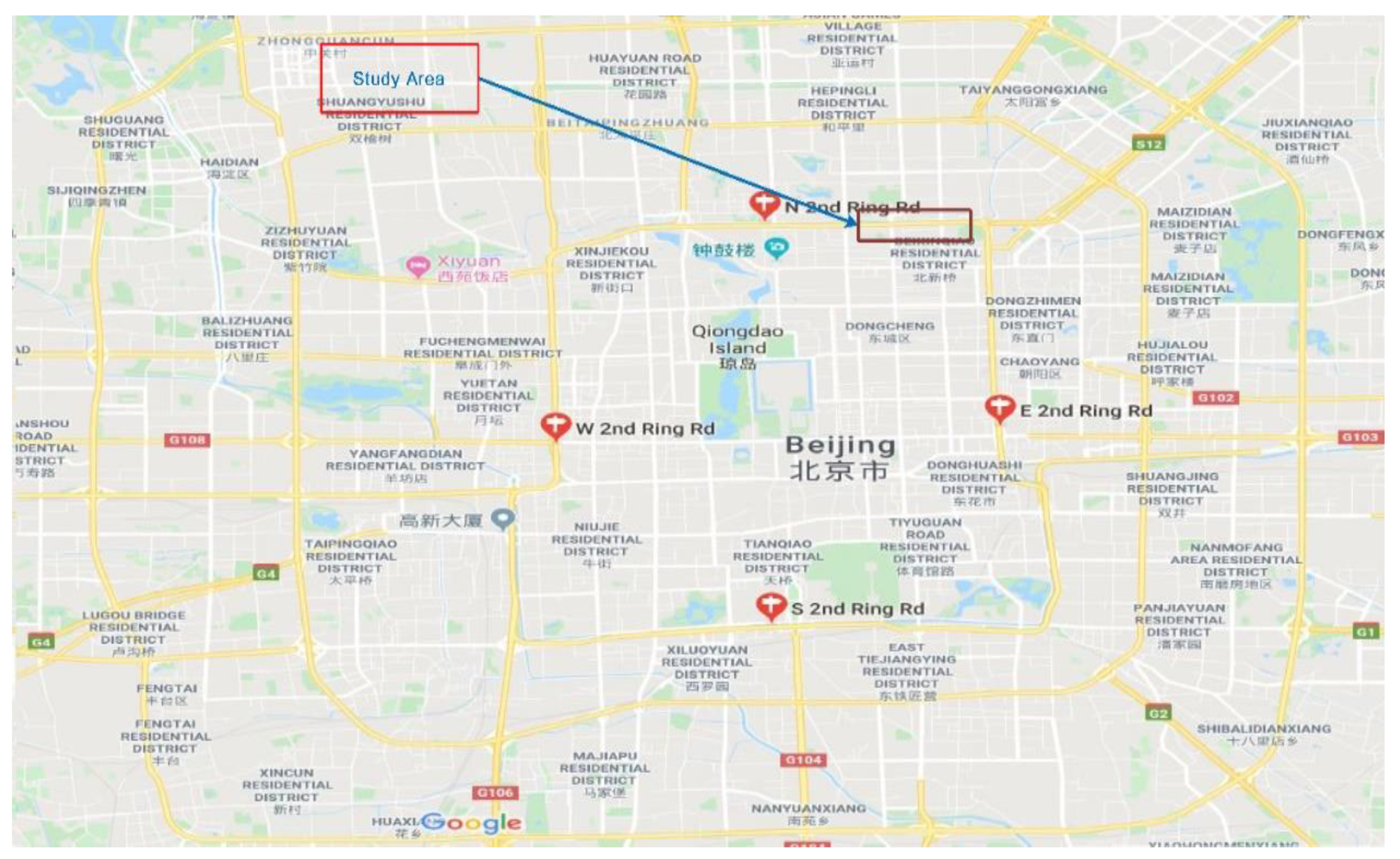
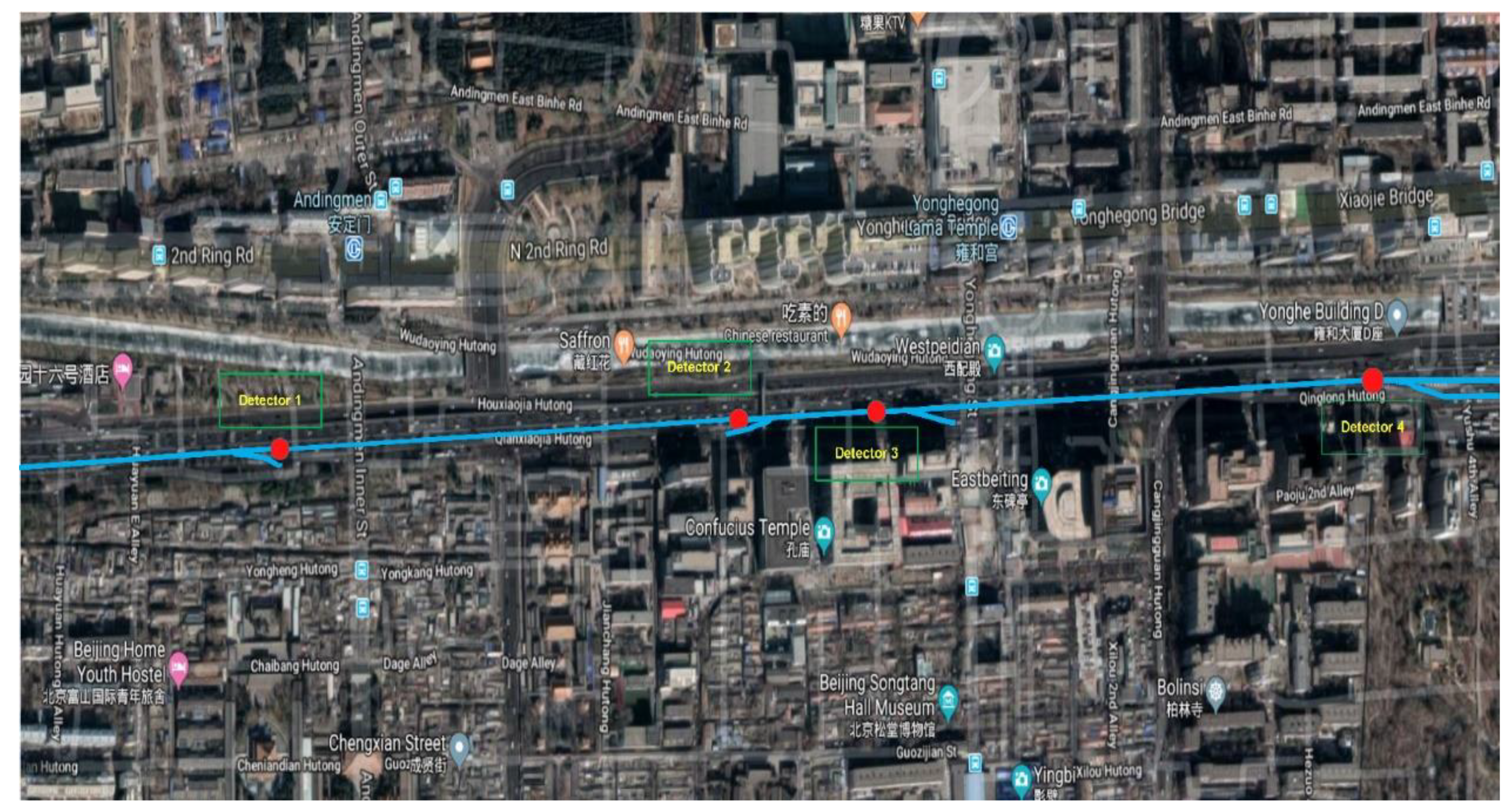
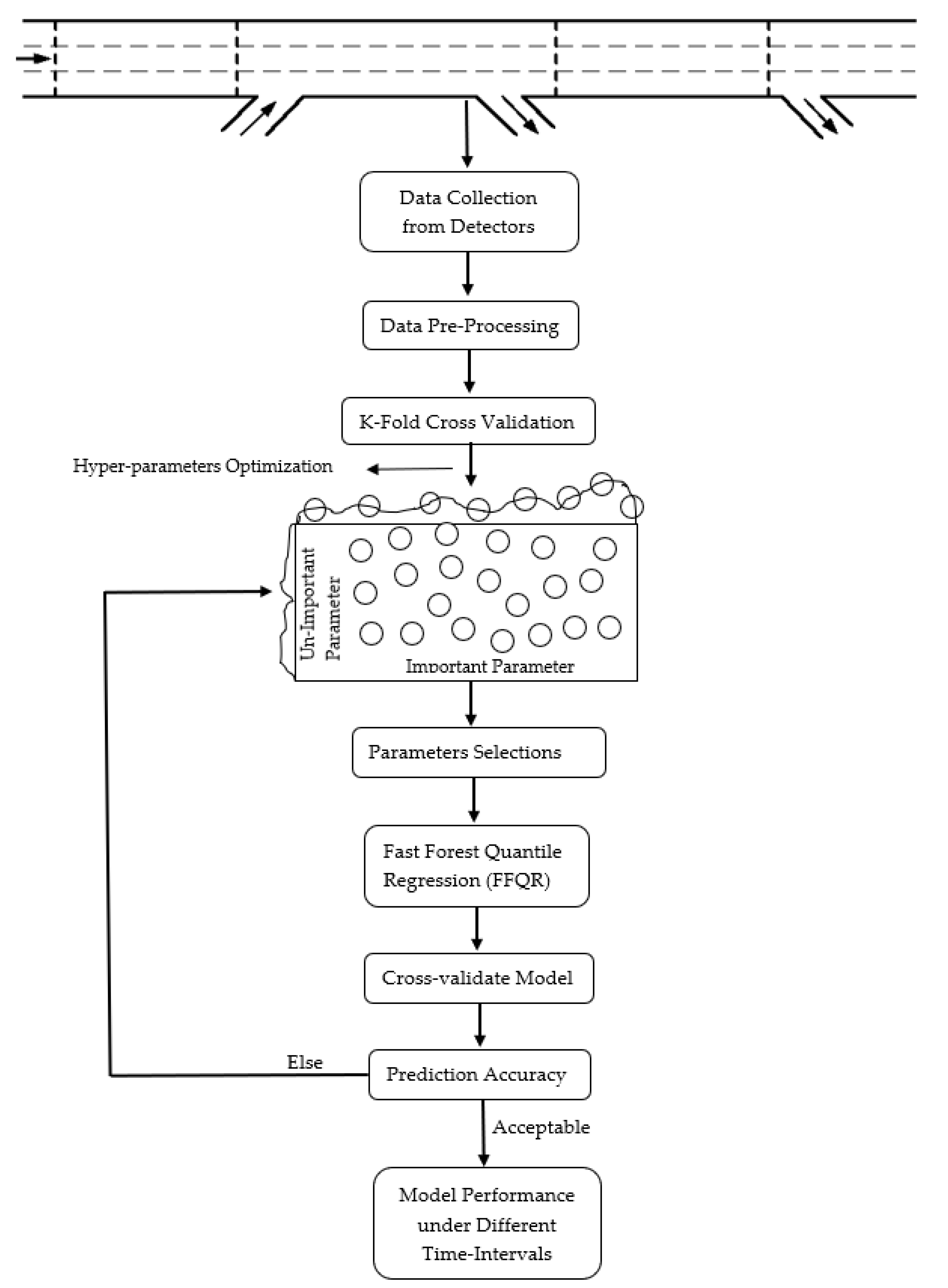
Numerous powerful traffic simulation tools are available to replicate realistic field driving conditions by incorporating appropriate parameters inputs. It was anticipated that very realistic outcomes can be achieved by enabling a precise geometric representation of conditions, the behavior of drivers, and vehicle features. A number of verifications have been initiated, involving examination of coded networks, so that the coded network can replicate current field conditions. Microscopic traffic simulation tool VISSIM was used to realistically simulate traffic conditions in the study area. However prior to the field conditions, it is essential to calibrate the driving behavior parameters for the traffic simulator using appropriate procedures as reported by a recent study [75]. After default parameter calibration and validation of a traffic simulator, multiple simulation runs were performed with different random seeds to ensure that the model worked as planned. A portion of Beijing’s 2nd freeway Ring Road (shown in Figure 1) was selected to verify the performance of the proposed approach. The length of the selected segment was 1.326 km. The 2nd freeway Ring Road is approximately 33 km and includes 37 on-ramps and 53 off-ramps. After getting the appropriate freeway architecture, the macroscopic characteristics (e.g., split ratio and demand flow) needed for the tuning of the complete microscopic simulator were identified. Using the VISSIM 2nd freeway Ring Road network simulation model, the traffic flow from around 06:00 a.m. to 12:00 p.m. has been further mimicked. The data was collected on a selected portion of 2nd freeway Ring Road from different loop detectors with different time intervals, including 05, 10, 15 min. The location of 2nd freeway Ring Road from detector 1 to detector 4 can be seen in Figure 2. Figure 3 presents the flow chart for sequential methodology.
4. Methodology
4.1. Fast Forest Qunatile Regression
There are various regression types. Regression models aim to fit a target variable that is expressed as a numerical vector. Nevertheless, statisticians have increasingly developed sophisticated regression techniques. Quantile regression enables to understand the predicted value distribution. FFQR is a powerful tree-based quantile regression model utilized in this study that is capable of predicting non-parameter distributions. FFQR uses decision trees to implement random forest quantile regression. Random forests (RF) can help prevent overfilling with decision trees. A tree ensemble is developed in a random forest using bagging to select a subset of random samples and training data characteristics, and then fit a decision tree into each data subset, unlike the algorithm of random forests, which averages all trees output. FFQR keeps all of the predicted labels in trees indicated by the quantile sample count parameter. It displays the distribution to allow the user to view the quantile values for the given instance. The main strength of FFQR is that in every leaf of every tree, all relevant observations are stored, not just their average like happens in a random forest. Instead of the conditional mean or average, it helps to predict conditional quantiles of a given instance. Tree-based quantile regression models such as fast forest quantiles regression have the additional advantage that they can be used to predict non-parametric distributions. In general, RF combines several regression trees into an ensemble to generate more accurate regressions by extracting many bootstrap samples from the original training data and fitting each sample with a tree [76].
In FFQR, traffic prediction problem could be formalized as: let be a measured value vector containing traffic measurements from a point of traffic network indexed by at time . The vector could have travel speed component measured by a specific loop detector indexed by . The datasets further divided into three sets, training, validation, and testing. Firstly, the training procedure uses two sets, whilst the third sets evaluates the capacity of predicting trained FFQR. In the RF, predicted outcomes for , new data samples resulting from predictors, , are modelled as a weighted average of responses , training data samples, with weights given in Equation (1), [77]. In particular, we consider the conditional distribution function (in Equation (2)) of response variable conditioned on the specific values of the predictor variable .
The estimated conditional distribution function is then given below (Equation (3)) Furthermore, the quantile is predicted by Equation (4).
Each RF is comprised of several trees. Every tree is grown by repeatedly splitting the training data by a bootstrap sample. Every split is a predictor value. Splitting frequently happens until the partition has reached a minimum number of observations. At that point, the partition becomes reach a terminal node. The average overall trees provide predictions that depend on the complete set of training data, including responses and predictors. Random forests provide an accurate and consistent estimation of the conditional mean of the variable response. FFQR is an overall random forest generalization that provides a robust, non-linear, and non-parametric method to estimate conditional quantities [78]. Besides, FFQR provides a robust, non-linear, and non-parametric method to estimate conditional quantities. On the other hand, random forests estimated the conditional mean, while FFQR gives an estimation of the entire conditional distribution. A brief overview of the Algorithm 1 is given below [78].
| Algorithm 1. Identification Algorithm |
|
The model depends on several parameters, which are essential for the efficacy of the model. In order to find improved results and high accuracy, we used the random grid as a hyperparameters optimization for FFQR. The range of best combination for hyperparameters optimization used for different prediction horizons are given in Table 1,
The above listed tuned-optimized hyperparameters were achieved using 10-fold cross-validation. For each prediction horizon, the number of iterations performed was 18. The FFQR via random grid implemented in Azure machine learning studio.
4.2. Model Evaluation
Quantile Loss functions proved to be useful for the prediction of an interval instead of only point-predictions. Also, quantile loss is simply an extension of mean absolute error (MAE). The performance evaluation metrics used in this study were quantile loss and root mean squared errors (RMSE). The metrics were calculated from the below equations;
where is the ground truth, is the predicted output, is the selected quantile and is the number of observations.
5. Results and Discussion
5.1. Quantile Loss for Different Time Horizon
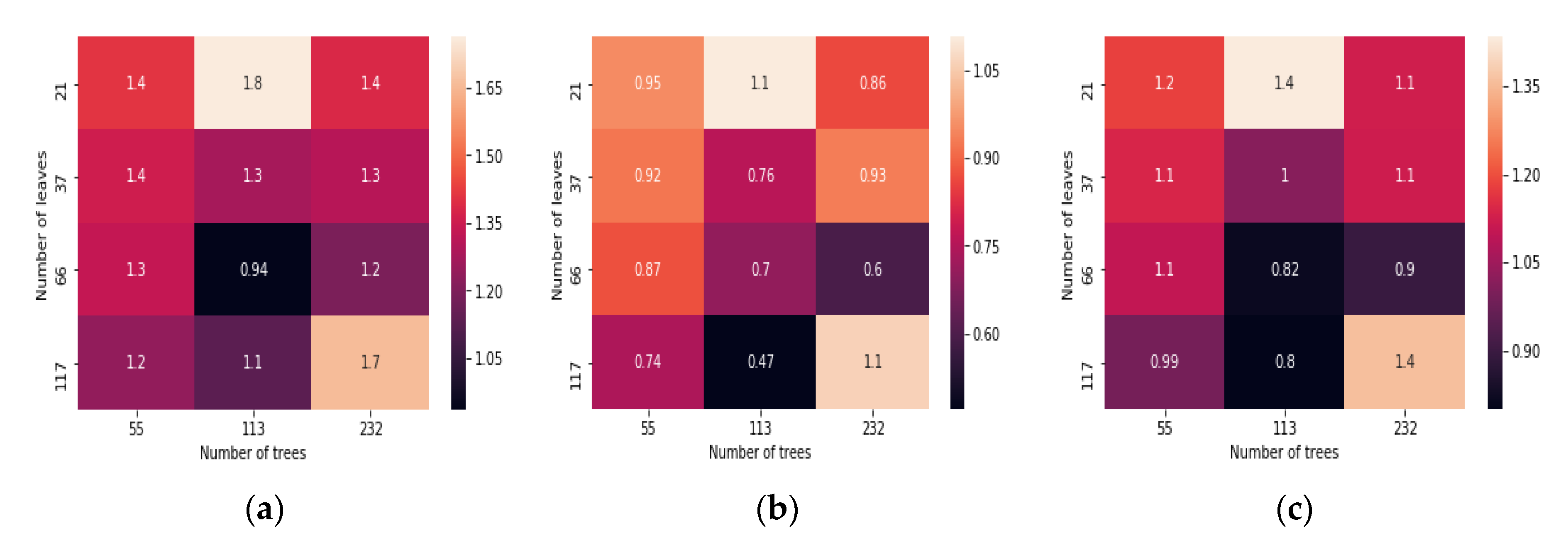
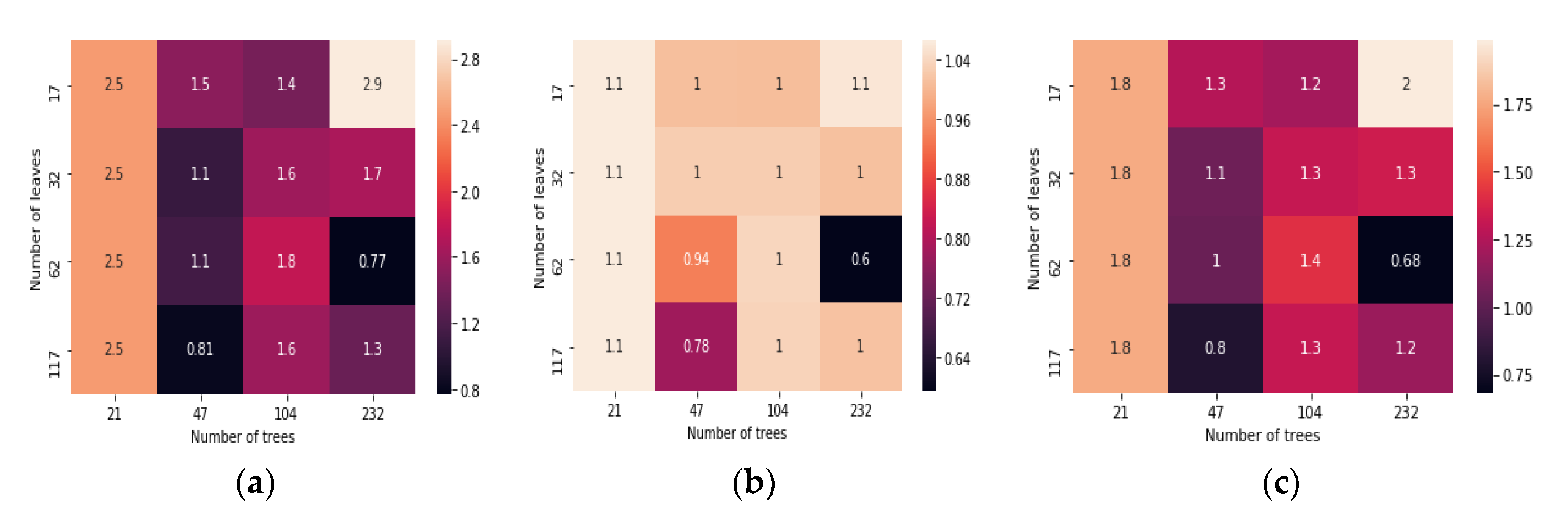
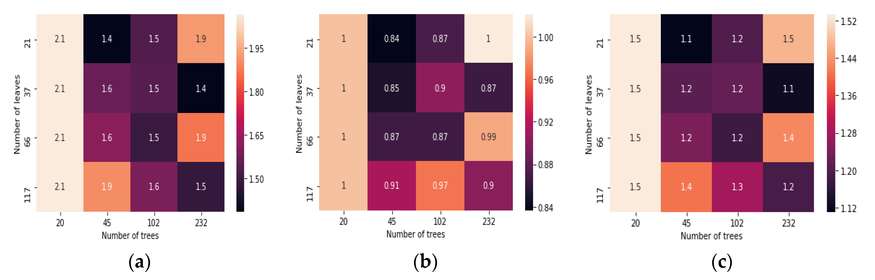
The hyper tuning parameters included for mean prediction, 0.07 quantile interval, and 0.95 quantile interval are the number of trees, number of leaves, minimum leaf instances, bagging fraction, and feature fraction. Figure 4 shows the quantile loss of detector 4 for 15 min prediction horizons, which are number of trees and a number of leaves. The quantile loss obtained for the mean prediction, 0.07 quantile, and 0.95 quantiles were 0.8007, 0.471, and 0.94, respectively. Figure 5 presents the detector 4 quantile loss for 10 min prediction horizons which were obtained for mean prediction, 0.07, and 0.95. The achieved values for a number of trees and the number of leaves is 0.68, 0.77, and 0.60. Similarly, Figure 6 indicates the quantile loss of detector 4 achieved for 5 min prediction horizons for mean prediction, 0.07, and 0.95 were 1.1, 1.4, and 0.84, respectively.
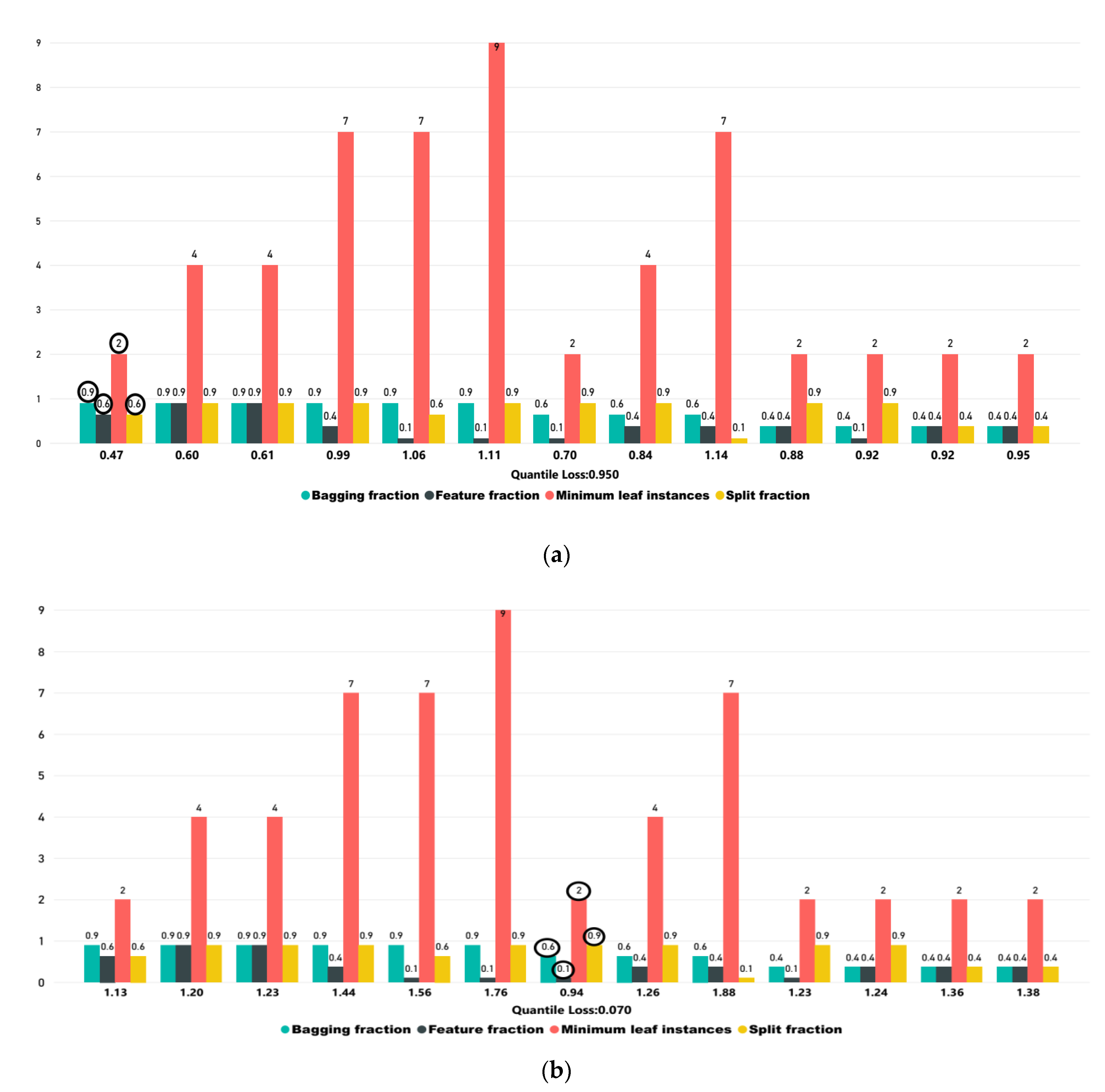
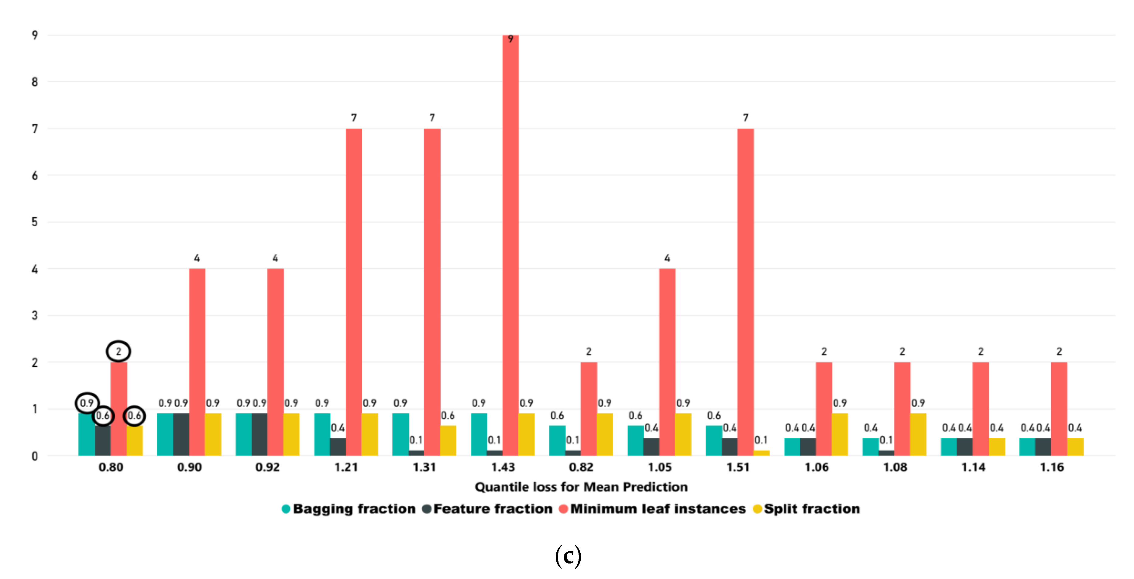
Figure 7a depicts the impact of minimum leaf instances, bagging fraction, split fraction, and feature fraction on quantile loss for 0.95 interval, which was achieved when the quantile loss was 0.47. The values achieved for minimum leaf instances, bagging fraction, split fraction, and feature fraction was 2, 0.9, 0.6, and 0.6, respectively. Figure 7b,c indicate the quantile loss for 0.07 interval and mean prediction, which was obtained for 0.94 and 0.80, respectively. The obtained values of 0.07 quantile for minimum leaf instances, bagging fraction, split fraction, and feature fraction were 2, 0.6, 0.9, and 0.1, respectively. Similarly, Figure 8c shows the achieved values of mean prediction for minimum leaf instances, bagging fraction, split fraction and feature fraction were 2, 0.9, 0.6, and 0.6, respectively. In Figure 7a–c, the encircled values show the values of the best-tuned parameters for mean prediction with less quantile loss, which was obtained for 10-fold cross-validation.
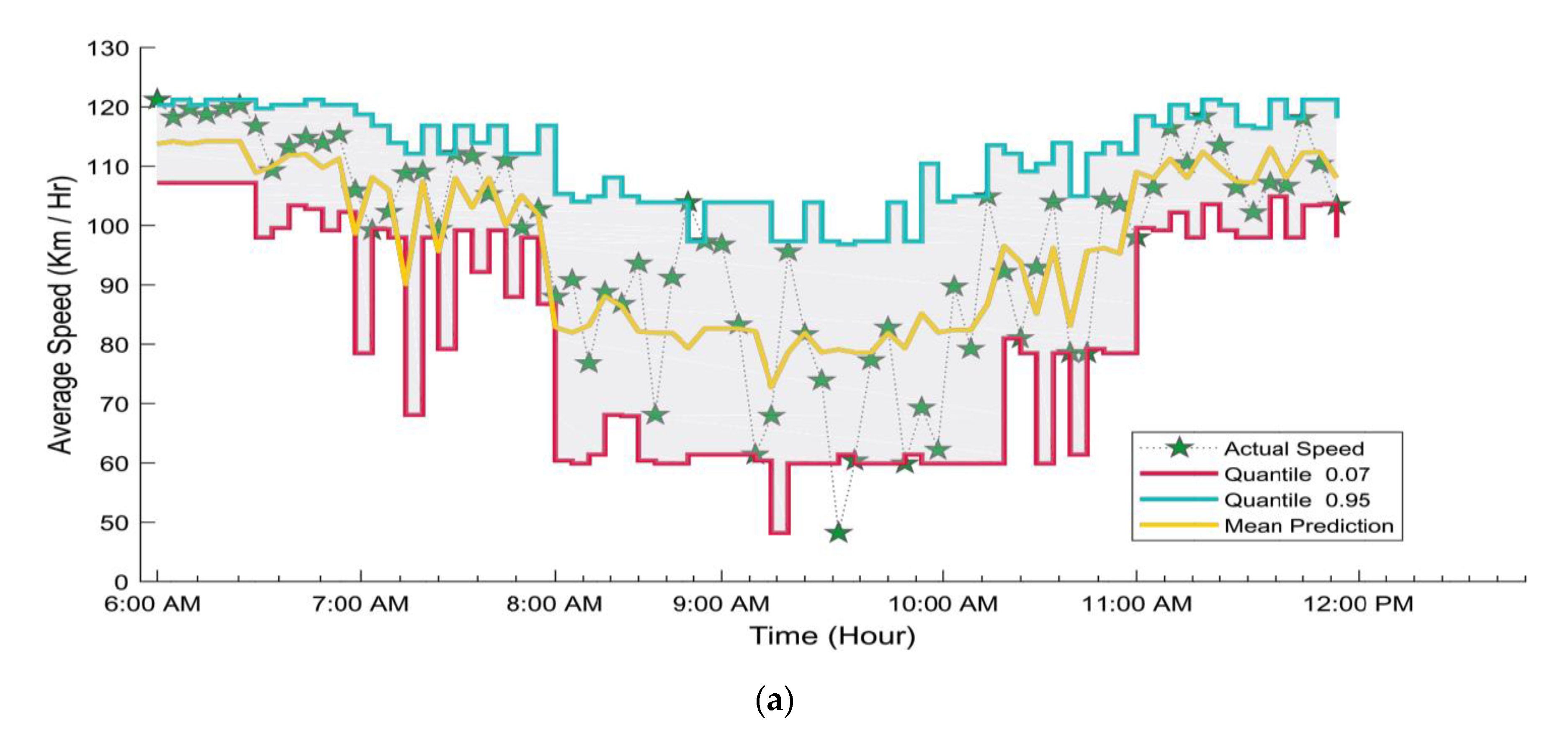
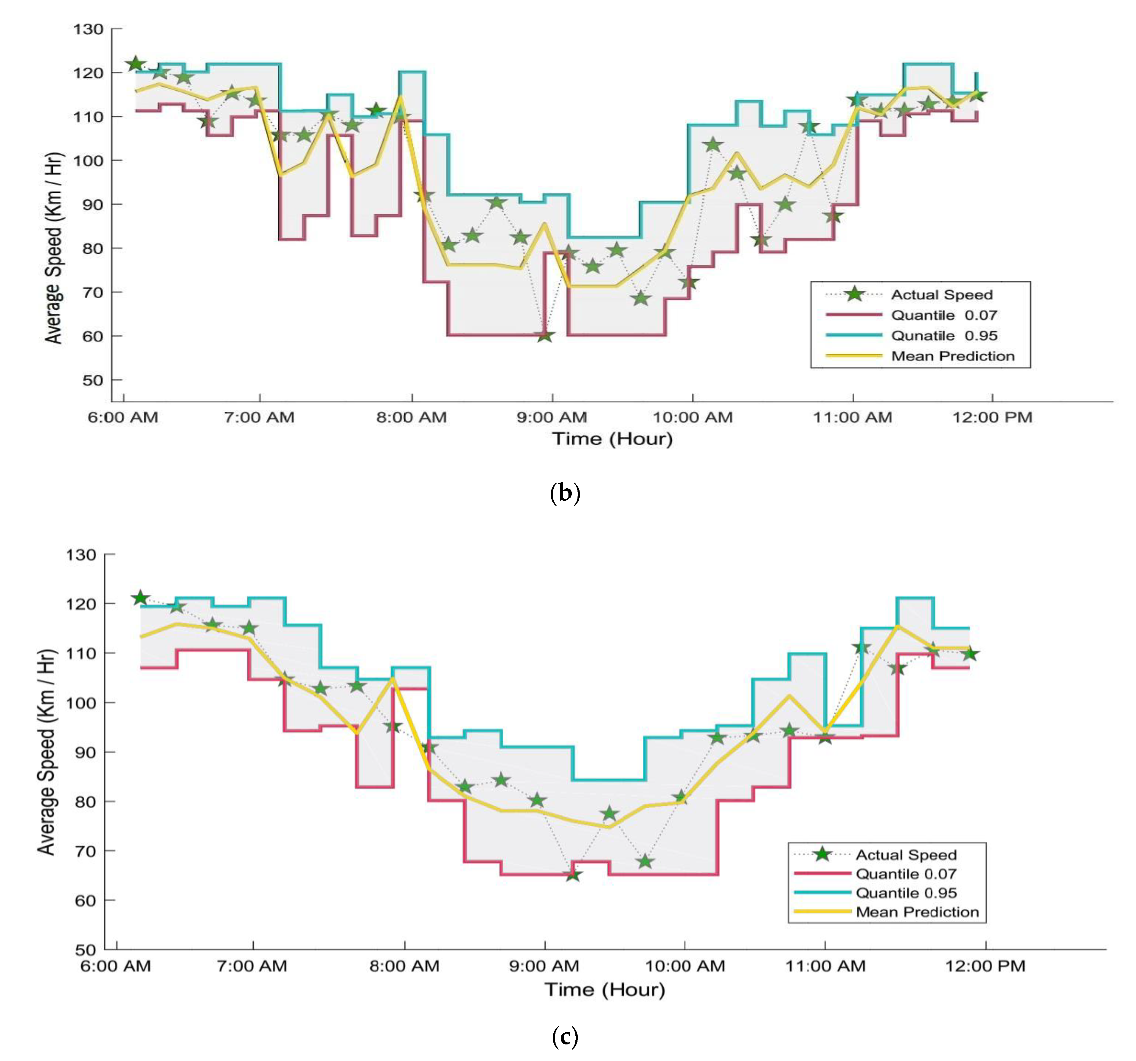
Figure 8 shows the predicted trends measured for detector 4 under different time intervals during morning peak hours and off-peak hours. It also indicates the actual mean prediction, 0.07, and 0.95 quantiles for 5, 10, and 15 min prediction horizons. We find that mean travel speed prediction, 0.07, and 0.95 quantiles were close to the actual speed data in the period of off-peak between (6:00 a.m. to 7:30 a.m. and 10:30 a.m. to 12:00 p.m.). In addition, results showed that the prediction accuracy for off-peak hours (normal time) is better than the peak hours’ period because the traffic flow is more stable during normal time than the peak time.
5.2. Model Perfrmance under Different Time Intervals
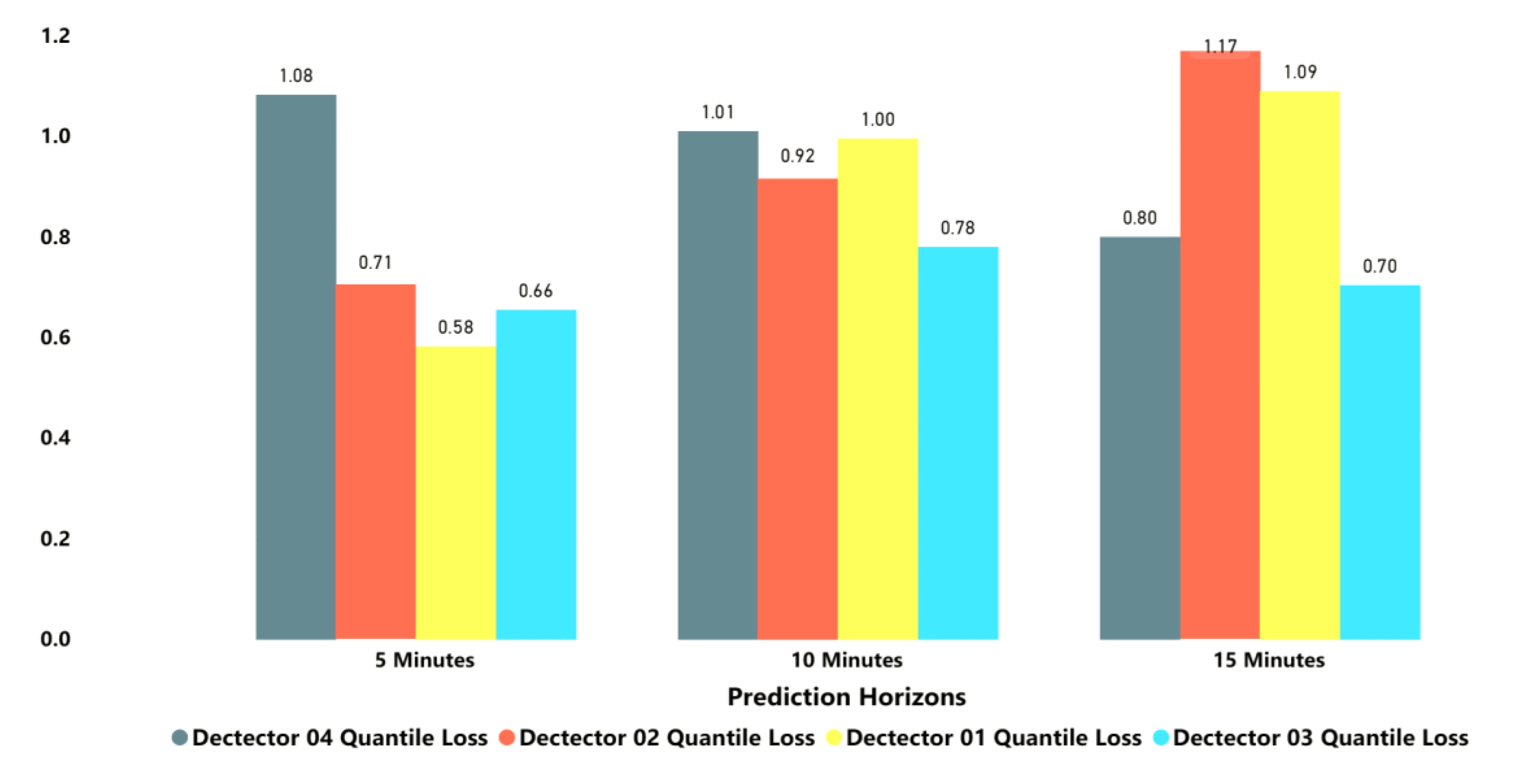
The impact of data collection time intervals on the prediction of short-term travel speed accuracy is essential. FFQR was used to predict short term travel speed at different time intervals (i.e., 5, 10, and 15 min). The quantile loss of mean prediction for data collected in different time intervals from different loop detectors can be seen in Figure 9, which shows a similar trend for detector 3 and detector 4, as time-horizons increased the quantile loss decreased. It can be observed from Figure 9 that the proposed FFQR yielded robust travel speed prediction outcomes with varying time-horizons, particularly at larger time intervals. The prediction accuracy increased for increasing the time intervals, as shown in Figure 9. The model performed better as shown in Table 2 and Table 3 with lower quantiles loss and RMSE for loop detectors at different time intervals, demonstrating the traffic speed pattern characteristics over time. For example, the mean quantile loss and RMSE for all loop detectors for time intervals of 10 min are 0.941 and 11.26, respectively. In contrast, the mean quantile loss and RMSE for all loop detectors for time interval of 15 min are 0.93 and 10.73 respectively. Despite the sophisticated and complex road conditions in the empirical test, model performance remained entirely satisfactory. The decrease in these two indicators, quantile loss and RMSE, indicated the improvement in the short-term speed prediction. Further, it may be noted from the results that the suggested model yielded desirable travel speed prediction results with low RMSE. These results are indicative of the fact that increasing the time interval for data collection could reduce traffic uncertainty, therefore the speed pattern is more stable and also predictable [79]. Additionally, the higher accuracy relationship with increased time intervals for data collection is aligned with many other legitimate prediction approaches [80]. Similar studies conducted suggest that prediction accuracy is inversely proportional to data collection time-horizons. For example, in a study the accuracy obtained (in term of RMSE) for traffic speed prediction using Elman NN for 1 min and 4 min were 10.79 and 12.92, which was less reliable relating to our obtained prediction accuracy for different time-horizons [32]. In addition, researchers have compared various models such as SVR, ANN, bayesian regularized neural network (BRNN) and SARIMA to forecast short-term speed and achieved prediction accuracy estimates comparable to our proposed method. In these studies, authors have demonstrated the predicted travel speed trend during off-peak hours and peak hours of the day and captured traffic nonlinearity in arbitrary time horizons [81,82,83].
6. Conclusions, Study Limitations, and Future Work
6.1. Conclusions
The objective of this study was to predict short-term travel speed under different time-horizons, which is extremely essential for travel route planning, real-time proactive traffic control, and management in ITS. Existing literature on the topic was reviewed, which revealed that previous studies have mostly focused on time-series, statistical regression, and conventional artificial intelligence techniques (such as ANN, SVM). However, prediction accuracy from time-series methods are relatively low, whereas traditional AI approaches have too shallow architecture to capture the non-linear, stochastic, and intricate characteristics of traffic flow. Thus, we proposed a novel FFQR model for short-term travel speed forecasting under multiple data collection time-ahead horizons. FFQR is an ensemble technique having relatively deep architecture that combines several regression trees to yield more accurate regressions estimates for a predictor variable. The proposed method was applied using loop detectors data based on a microscopic traffic simulator along a freeway segment on 2nd Ring Road in Beijing. The results showed that the FFQR model performed well in predicting short-term travel speed, particularly at larger time-horizons. The study findings also showed that speed prediction error quantified in terms of quantiles loss on average ranged between 0.58 and 1.18. It was also noted that the proposed FFQR model was efficient in capturing the observed variations in field speed data. Prediction results demonstrated the adequacy and robustness of the proposed approach under different data collection time scenarios. Hence, travel speed prediction from the FFQR model could serve as useful guidance for policy and decisions makers particularly in the study area (city of Beijing) as wells as travelers in the city for efficient operations and commute through urban metropolitans.
Future studies should focus on exploring the influence of other important external factors such as weather and traffic incidents to enhance prediction accuracy of travel speed. In addition, current study could be extended to data collected from network-wide loop detectors or sensors considering the spatial information of travel to evaluate the adequacy of the proposed approach. Lastly, future studies could concentrate on additional advanced optimization techniques to explore more appropriate parameter combinations for the current proposed model, and to achieve more accurate short-term travel speed prediction outcomes.
6.2. Study Limitations
This study has a few limitations that must be acknowledged. First, the current study utilized speed data from a single road segment; however, traffic on adjacent road segments may affect the predicted speed performance on the target road segment. Second, uncertainty in travel speed prediction emerged as an inevitable issue due to the stochastic nature of traffic data. Third, this study used speed data from fixed location loop detectors that are not reliable for collecting such data network-wide. Data from GPS navigation devices and RTMS could serve as a potentially more valuable alternative for capturing instantaneous speed in a congested urban network. Finally, this research utilized VISSIM simulation data to justify the efficacy of the proposed approach, however, it should be noted that there are some limits on the developed simulated urban freeway network model.
Author Contributions
Conceptualization, M.Z. and Y.C.; methodology, M.Z., and Y.C.; software, M.Z. and A.J.; validation, M.Z., Y.C., and A.J.; formal analysis, M.Z., Y.C., and A.J.; investigation, M.Z., Y.C., and A.J.; resources, M.Z. and Y.C.; writing—original draft preparation, M.Z. and Y.C.; writing—review and editing, M.Z., A.J., Y.C., and C.Z.M.; visualization, M.Z. and C.Z.M. All authors have read and agreed to the published version of the manuscript.
Funding
The work was supported by the National Natural Science Foundation of China (Grant No. 61573030).
Acknowledgments
The authors appreciate and acknowledge the support of BJUT. The authors also acknowledge the support and guidance of Pawel Gora (Research Group Tensor Cell, University of Warsaw, Poland).
Conflicts of Interest
The authors declare no conflict of interest.
References
- Huang, Z.; Xia, J.; Li, F.; Li, Z.; Li, Q. A Peak Traffic Congestion Prediction Method Based on Bus Driving Time. Entropy 2019, 21, 709. [Google Scholar] [CrossRef] [Green Version]
- Liu, S.; Triantis, K.P.; Sarangi, S. A framework for evaluating the dynamic impacts of a congestion pricing policy for a transportation socioeconomic system. Transp. Res. Part A Policy Pract. 2010, 44, 596–608. [Google Scholar] [CrossRef]
- Zheng, Y.; Capra, L.; Wolfson, O.; Yang, H. Urban Computing: Concepts, Methodologies, and Applications. ACM Trans. Intell. Syst. Technol. 2014. [Google Scholar] [CrossRef]
- Bani Younes, M.; Boukerche, A. A Performance Evaluation of an Efficient Traffic Congestion Detection Protocol (ECODE) for Intelligent Transportation Systems. Ad Hoc Netw. 2015, 24, 317–336. [Google Scholar] [CrossRef]
- Wang, M.Q.; Harvey, H. Chinese transport: achievements and challenges of transport policies. Mitig. Adapt. Strateg. Glob. Chang. 2015, 20, 623–626. [Google Scholar] [CrossRef]
- National Bureau of Statistics of China. China Statistical Yearbook 2019; National Bureau of Statistics of China: Beijing, China, 2019.
- Sachon, M.R.J.; Zhang, D.; Zhang, Y.; Castillo, C. The Chinese Automotive Industry in 2016; Universidad de Navarra: Pamplona, Spain, 2016. [Google Scholar]
- Levy, J.I.; Buonocore, J.J.; Stackelberg, K. von The Public Health Costs of Traffic Congestion A Health Risk Assessment. Environ. Heal. 2010, 9, 1–12. [Google Scholar] [CrossRef] [PubMed] [Green Version]
- Luo, J. Cities around the World: Struggles and Solutions to Urban Life [2 Volumes]; ABC-CLIO: Santa Barbara, CA, USA, 2019; ISBN 144085386X. [Google Scholar]
- Kim, Y.; Kang, W.; Park, M. Application of Traffic State Prediction Methods to Urban Expressway Network in the City of Seoul. J. East. Asia Soc. Transp. Stud. 2015, 11, 1885–1898. [Google Scholar]
- Mannini, L.; Carrese, S.; Cipriani, E.; Crisalli, U. On the Short-term Prediction of Traffic State: An Application on Urban Freeways in ROME. Transp. Res. Procedia 2015, 10, 176–185. [Google Scholar] [CrossRef]
- Long, K.; Yao, W.; Gu, J.; Wu, W.; Han, L.D. Predicting freeway travel time using multiple-source heterogeneous data integration. Appl. Sci. 2018, 9, 104. [Google Scholar] [CrossRef] [Green Version]
- Gmira, M.; Gendrea, M.; Lodi, A.; Jean-Yves Potvin, M. Travel Speed Prediction Based on Learning Methods for Home Delivery; Canada Excellence Research Chairs (CERC): Montréal, QC, Canada, 2018. [Google Scholar]
- Dauwels, J.; Aslam, A.; Asif, M.T.; Zhao, X.; Vie, N.M.; Cichocki, A.; Jaillet, P. Predicting traffic speed in urban transportation subnetworks for multiple horizons. In Proceedings of the 2014 13th International Conference on Control Automation Robotics & Vision (ICARCV), Singapore, 10–12 December 2014; pp. 547–552. [Google Scholar]
- Ishak, S.; Al-Deek, H. Performance evaluation of short-term time-series traffic prediction model. J. Transp. Eng. 2002, 128, 490–498. [Google Scholar] [CrossRef]
- Sun, H.; Liu, H.X.; Xiao, H.; He, R.R.; Ran, B. Use of local linear regression model for short-term traffic forecasting. Transp. Res. Rec. 2003, 1836, 143–150. [Google Scholar] [CrossRef]
- Zhang, S.; Yao, Y.; Hu, J.; Zhao, Y.; Li, S.; Hu, J. Deep autoencoder neural networks for short-term traffic congestion prediction of transportation networks. Sensors (Switzerland) 2019, 19, 2229. [Google Scholar] [CrossRef] [PubMed] [Green Version]
- Park, J.; Li, D.; Murphey, Y.L.; Kristinsson, J.; McGee, R.; Kuang, M.; Phillips, T. Real time vehicle speed prediction using a neural network traffic model. In Proceedings of the 2011 International Joint Conference on Neural Networks, San Jose, CA, USA, 31 July–5 August 2011; pp. 2991–2996. [Google Scholar]
- Jiang, H.; Zou, Y.; Zhang, S.; Tang, J.; Wang, Y. Short-term speed prediction using remote microwave sensor data: machine learning versus statistical model. Math. Probl. Eng. 2016, 2006. [Google Scholar] [CrossRef] [Green Version]
- Sun, H.; Liu, H.X.; Xiao, H.; He, R.R.; Ran, B. Short term traffic forecasting using the local linear regression model. In Proceedings of the 82nd Annual Meeting of the Transportation Research Board, Washington, DC, USA, 12–16 January 2003. [Google Scholar]
- Van Hinsbergen, C.P.; Van Lint, J.W.; Sanders, F.M. Short term traffic prediction models. In Proceedings of the 14th World Congress on Intelligent Transport Systems (ITS), Beijing, China, 9–13 October 2007. [Google Scholar]
- Pan, T.L.; Sumalee, A.; Zhong, R.-X.; Indra-Payoong, N. Short-term traffic state prediction based on temporal–spatial correlation. IEEE Trans. Intell. Transp. Syst. 2013, 14, 1242–1254. [Google Scholar] [CrossRef]
- Jamal, A.; Rahman, M.T.; Al-ahmadi, H.M. The Dilemma of Road Safety in the Eastern Province of Saudi Arabia: Consequences and Prevention Strategies. Int. J. Environ. Res. Public Helath 2019, 17, 157. [Google Scholar] [CrossRef] [Green Version]
- Avineri, E.; Prashker, J.N. The impact of travel time information on travelers’ learning under uncertainty. Transportation (Amst) 2006, 33, 393–408. [Google Scholar] [CrossRef]
- Zheng, F.; Van Zuylen, H. Uncertainty and Predictability of Urban Link Travel Time: Delay Distribution–Based Analysis. Transp. Res. Rec. 2010, 2192, 136–146. [Google Scholar] [CrossRef]
- Noland, R.; Small, K.A. Travel-time uncertainty, departure time choice, and the cost of morning commutes. Transp. Res. Rec. 1995, 150–158. [Google Scholar]
- Zhu, D.; Shen, G.; Liu, D.; Chen, J.; Zhang, Y. FCG-aspredictor: An approach for the prediction of average speed of road segments with floating car GPS data. Sensors (Switzerland) 2019, 19, 4967. [Google Scholar] [CrossRef] [Green Version]
- Anil Rao, Y.G.; Sujith Kumar, N.; Amaresh, H.S.; Chirag, H.V. Real-time speed estimation of vehicles from uncalibrated view-independent traffic cameras. In Proceedings of the IEEE Region 10 Annual International Conference, TENCON 2015, Macao, China, 1–4 November 2015. [Google Scholar]
- Yu, D.; Liu, C.; Wu, Y.; Liao, S.; Anwar, T.; Li, W.; Zhou, C. Forecasting short-term traffic speed based on multiple attributes of adjacent roads. Knowl-Based Syst. 2019, 163, 472–484. [Google Scholar] [CrossRef]
- Siuhi, S.; Mwakalonge, J. Opportunities and challenges of smart mobile applications in transportation. J. Traffic Transp. Eng. (English Ed.) 2016, 3, 582–592. [Google Scholar] [CrossRef] [Green Version]
- Yu, X.; Prevedouros, P.D. Performance and Challenges in Utilizing Non-Intrusive Sensors for Traffic Data Collection. Adv. Remote Sens. 2013, 2, 45–50. [Google Scholar] [CrossRef] [Green Version]
- Ma, X.; Tao, Z.; Wang, Y.; Yu, H.; Wang, Y. Long short-term memory neural network for traffic speed prediction using remote microwave sensor data. Transp. Res. Part C Emerg. Technol. 2015, 54, 187–197. [Google Scholar] [CrossRef]
- Zhang, J.; He, S.; Wang, W.; Zhan, F. Accuracy Analysis of Freeway Traffic Speed Estimation Based on the Integration of Cellular Probe System and Loop Detectors. J. Intell. Transp. Syst. Technol. Plan. Oper. 2015, 19, 411–426. [Google Scholar] [CrossRef]
- Katsuki, T.; Morimura, T.; Inoue, M. Traffic Velocity Estimation from Vehicle Count Sequences. IEEE Trans. Intell. Transp. Syst. 2017, 18, 1700–1712. [Google Scholar] [CrossRef]
- Deng, B.; Denman, S.; Zachariadis, V.; Jin, Y. Estimating traffic delays and network speeds from low-frequency GPS taxis traces for urban transport modelling. Eur. J. Transp. Infrastruct. Res. 2015, 15, 639–661. [Google Scholar]
- Dendrinos, D.S. Traffic-flow dynamics: A search for chaos. Chaos Solitons Fract. 1994, 4, 605–617. [Google Scholar] [CrossRef]
- Seo, T.; Bayen, A.M.; Kusakabe, T.; Asakura, Y. Traffic state estimation on highway: A comprehensive survey. Annu. Rev. Control 2017, 43, 128–151. [Google Scholar] [CrossRef] [Green Version]
- Bergstra, J.; Bardenet, R.; Bengio, Y.; Kégl, B. Algorithms for hyper-parameter optimization. In Proceedings of the Advances in Neural Information Processing Systems 24: 25th Annual Conference on Neural Information Processing Systems, Granada, Spain, 12–14 December 2011. [Google Scholar]
- van Hinsbergen, C.P.I.; van Lint, J.W.C.; van Zuylen, H.J. Bayesian committee of neural networks to predict travel times with confidence intervals. Transp. Res. Part C Emerg. Technol. 2009, 17, 498–509. [Google Scholar] [CrossRef]
- Kumar, S.V.; Vanajakshi, L. Short-term traffic flow prediction using seasonal ARIMA model with limited input data. Eur. Transp. Res. Rev. 2015, 7, 1–9. [Google Scholar] [CrossRef] [Green Version]
- Ahmed, M.S.; Cook, A.R. Analysis of Freeway Traffic Time-Series Data By Using Box-Jenkins Techniques. Transp. Res. Rec. 1979, 722, 1–9. [Google Scholar]
- Ross, P. Exponential filtering of traffic data. Transp. Res. Rec. 1982, 869, 43–49. [Google Scholar]
- Zhang, Y.; Zhang, Y.; Haghani, A. A hybrid short-term traffic flow forecasting method based on spectral analysis and statistical volatility model. Transp. Res. Part C Emerg. Technol. 2014, 43, 65–78. [Google Scholar] [CrossRef]
- Tchrakian, T.T.; Basu, B.; O’Mahony, M. Real-time traffic flow forecasting using spectral analysis. IEEE Trans. Intell. Transp. Syst. 2012, 13, 519–526. [Google Scholar] [CrossRef]
- Levin, M.; Tsao, Y.-D. On forecasting freeway occupancies and volumes (abridgment). Transp. Res. Rec. 1980, 722, 47–49. [Google Scholar]
- Nihan, N.; Holmesland, K. Use of the Box and Jekins Time Series Technique in Traffic Forecatsing. Transportation (Amst) 1980, 9, 125–143. [Google Scholar] [CrossRef]
- Karlaftis, M.G.; Vlahogianni, E.I. Memory properties and fractional integration in transportation time-series. Transp. Res. Part C Emerg. Technol. 2009, 17, 444–453. [Google Scholar] [CrossRef]
- der Voort, M.; Dougherty, S.W. Combining Kohen Maps with Arima Time Series Models to Forecats Traffic Flow. Transp. Res. Part C Emerg. Technol. 1996, 5, 307–318. [Google Scholar] [CrossRef] [Green Version]
- Williams, B.M.; Hoel, L.A. Modeling and forecasting vehicular traffic flow as a seasonal ARIMA process: Theoretical basis and empirical results. J. Transp. Eng. 2003, 129, 664–672. [Google Scholar] [CrossRef] [Green Version]
- Lippi, M.; Bertini, M.; Frasconi, P. Short-term traffic flow forecasting: An experimental comparison of time-series analysis and supervised learning. IEEE Trans. Intell. Transp. Syst. 2013, 14, 871–882. [Google Scholar] [CrossRef]
- Dunne, S.; Ghosh, B. Regime-based short-term multivariate traffic condition forecasting algorithm. J. Transp. Eng. 2012, 138, 455–466. [Google Scholar] [CrossRef]
- Chan, K.Y.; Dillon, T.S.; Singh, J.; Chang, E. Neural-network-based models for short-term traffic flow forecasting using a hybrid exponential smoothing and levenberg-marquardt algorithm. IEEE Trans. Intell. Transp. Syst. 2012, 13, 644–654. [Google Scholar] [CrossRef]
- Huang, S.-H.; Ran, B. An Application of Neural Network on Traffic Speed Prediction Under Adverse Weather Condition. In Proceedings of the 82nd Annual Meeting of the Transportation Research Board, Washington, DC, USA, 12–16 January 2003; pp. 1–21. [Google Scholar]
- Chen, H.; Grant-Muller, S. Use of sequential learning for short-term traffic flow forecasting. Transp. Res. Part C Emerg. Technol. 2001, 9, 319–336. [Google Scholar] [CrossRef]
- Ma, X.; Dai, Z.; He, Z.; Ma, J.; Wang, Y.; Wang, Y. Learning traffic as images: A deep convolutional neural network for large-scale transportation network speed prediction. Sensors (Switzerland) 2017, 17, 818. [Google Scholar] [CrossRef] [Green Version]
- El Faouzi, N.-E. Nonparametric traffic flow prediction using kernel estimator. In Proceedings of the Transportation and Traffic Theory. In Proceedings of the 13th International Symposium on Transportation and Traffic Theory, Lyon, France, 24–26 July 1996. [Google Scholar]
- Habtemichael, F.G.; Cetin, M. Short-term traffic flow rate forecasting based on identifying similar traffic patterns. Transp. Res. Part C Emerg. Technol. 2016, 66, 61–78. [Google Scholar] [CrossRef]
- Davis, B.G.A.; Member, A.; Nihan, N.L. Nonparametric regression and short-term freeway traffic forecasting. J. Transp. Eng. 1991, 117, 178–188. [Google Scholar] [CrossRef]
- Jeong, Y.S.; Byon, Y.J.; Castro-Neto, M.M.; Easa, S.M. Supervised weighting-online learning algorithm for short-term traffic flow prediction. IEEE Trans. Intell. Transp. Syst. 2013, 14, 1700–1707. [Google Scholar] [CrossRef]
- Yao, B.; Chen, C.; Cao, Q.; Jin, L.; Zhang, M.; Zhu, H.; Yu, B. Short-Term Traffic Speed Prediction for an Urban Corridor. Comput. Civ. Infrastruct. Eng. 2017, 32, 154–169. [Google Scholar] [CrossRef]
- Zheng, W.; Lee, D.H.; Shi, Q. Short-term freeway traffic flow prediction: Bayesian combined neural network approach. J. Transp. Eng. 2006, 132, 114–121. [Google Scholar] [CrossRef] [Green Version]
- Dimitriou, L.; Tsekeris, T.; Stathopoulos, A. Adaptive hybrid fuzzy rule-based system approach for modeling and predicting urban traffic flow. Transp. Res. Part C Emerg. Technol. 2008, 16, 554–573. [Google Scholar] [CrossRef]
- Zhang, Y.; Liu, Y. Traffic forecasting using least squares support vector machines. Transportmetrica 2009, 5, 193–213. [Google Scholar] [CrossRef]
- Chen, X.Y.; Pao, H.K.; Lee, Y.J. Efficient traffic speed forecasting based on massive heterogenous historical data. In Proceedings of the 2014 IEEE International Conference on Big Data, Washington, DC, USA, 27–30 October 2014; pp. 10–17. [Google Scholar]
- Wang, J.; Shi, Q. Short-term traffic speed forecasting hybrid model based on Chaos-Wavelet Analysis-Support Vector Machine theory. Transp. Res. Part C Emerg. Technol. 2013, 27, 219–232. [Google Scholar] [CrossRef]
- Fusco, G.; Colombaroni, C.; Isaenko, N. Short-term speed predictions exploiting big data on large urban road networks. Transp. Res. Part C Emerg. Technol. 2016, 73, 183–201. [Google Scholar] [CrossRef]
- Fan, Q.; Wang, W.; Hu, X.; Hua, X.; Liu, Z. Space-Time Hybrid Model for Short-Time Travel Speed Prediction. Discret. Dyn. Nat. Soc. 2018, 2018. [Google Scholar] [CrossRef] [Green Version]
- Pozna, C.; Precup, R.-E.; Tar, J.K.; Škrjanc, I.; Preitl, S. New results in modelling derived from Bayesian filtering. Knowl-Based Syst. 2010, 23, 182–194. [Google Scholar] [CrossRef]
- Tang, J.; Liu, F.; Zou, Y.; Zhang, W.; Wang, Y. An Improved Fuzzy Neural Network for Traffic Speed Prediction Considering Periodic Characteristic. IEEE Trans. Intell. Transp. Syst. 2017, 18, 2340–2350. [Google Scholar] [CrossRef]
- Yu, R.; Li, Y.; Shahabi, C.; Demiryurek, U.; Liu, Y. Deep learning: A generic approach for extreme condition traffic forecasting. In Proceedings of the 17th SIAM International Conference on Data Mining, SDM 2017, Houston, TX, USA, 27–29 April 2017; pp. 777–785. [Google Scholar]
- Wang, J.; Chen, R.; He, Z. Traffic speed prediction for urban transportation network: A path based deep learning approach. Transp. Res. Part C Emerg. Technol. 2019, 100, 372–385. [Google Scholar] [CrossRef]
- Nowaková, J.; Prilepok, M.; Snášel, V. Medical image retrieval using vector quantization and fuzzy S-tree. J. Med. Syst. 2017, 41, 18. [Google Scholar] [CrossRef] [Green Version]
- Sarma, K.K. Neural network based feature extraction for assamese character and numeral recognition. Int. J. Artif. Intell. 2009, 2, 37–56. [Google Scholar]
- Gil, R.P.A.; Johanyák, Z.C.; Kovács, T. Surrogate model based optimization of traffic lights cycles and green period ratios using microscopic simulation and fuzzy rule interpolation. Int. J. Artif. Intell. 2018, 16, 20–40. [Google Scholar]
- Al-Ahmadi, H.M.; Jamal, A.; Reza, I.; Assi, K.J.; Ahmed, S.A. Using Microscopic Simulation-Based Analysis to Model Driving Behavior: A Case Study of Khobar-Dammam in Saudi Arabia. Sustainability 2019, 11, 3018. [Google Scholar] [CrossRef] [Green Version]
- Hastie, T.; Tibshirani, R.; Friedman, J. The Elements of Statistical Learning: Data Mining, Inference and Prediction; Springer Series and Statistics; Springer: Stanford, CA, USA, 2008. [Google Scholar]
- Booker, D.J.; Whitehead, A.L. Inside or outside: Quantifying extrapolation across river networks. Water Resour. Res. 2018, 54, 6983–7003. [Google Scholar] [CrossRef]
- Meinshausen, N. Quantile regression forests. J. Mach. Learn. Res. 2006, 7, 983–999. [Google Scholar]
- Guo, J.; Williams, B.M.; Smith, B.L. Data collection time intervals for stochastic short-term traffic flow forecasting. Transp. Res. Rec. 2007, 2024, 18–26. [Google Scholar] [CrossRef]
- Smith, B.L.; Ulmer, J.M. Freeway traffic flow rate measurement: Investigation into impact of measurement time interval. J. Transp. Eng. 2003, 129, 223–229. [Google Scholar] [CrossRef]
- Polson, N.G.; Sokolov, V.O. Deep learning for short-term traffic flow prediction. Transp. Res. Part C Emerg. Technol. 2017, 79, 1–17. [Google Scholar] [CrossRef] [Green Version]
- Qiu, C.; Wang, C.; Zuo, X.; Fang, B. A bayesian regularized neural network approach to short-term traffic speed prediction. In Proceedings of the 2011 IEEE International Conference on Systems, Man, and Cybernetics, Anchorage, AK, USA, 9–12 October 2011; pp. 2215–2220. [Google Scholar]
- Gülaçar, H.; Yaslan, Y.; Oktuğ, S.F. Short term traffic speed prediction using different feature sets and sensor clusters. In Proceedings of the NOMS 2016 IEEE/IFIP Network Operations and Management Symposium, Istanbul, Turkey, 25–29 April 2016; pp. 1265–1268. [Google Scholar]
Figure 1.
Study area: segment of freeway 2nd Ring Road (Google Map). (Note: the Chinese words in this map are just the name of some buildings (residential, temples etc.) and will not affect the meaning of this image).
Figure 1.
Study area: segment of freeway 2nd Ring Road (Google Map). (Note: the Chinese words in this map are just the name of some buildings (residential, temples etc.) and will not affect the meaning of this image).

Figure 2.
Location of 2nd Ring Road from detector 1 to 4 (Google Map). (Note: the Chinese words in this map are just the name of some buildings (residential, temples etc.) and will not affect the meaning of this image).
Figure 2.
Location of 2nd Ring Road from detector 1 to 4 (Google Map). (Note: the Chinese words in this map are just the name of some buildings (residential, temples etc.) and will not affect the meaning of this image).

Figure 3.
Flowchart for Methodology.

Figure 4.
Quantile loss at detector 4: (a) for 0.95 prediction horizon; (b) for 0.07 prediction horizon (c) for mean prediction horizon.
Figure 4.
Quantile loss at detector 4: (a) for 0.95 prediction horizon; (b) for 0.07 prediction horizon (c) for mean prediction horizon.

Figure 5.
Quantile loss at detector 4: (a) for 0.07 prediction horizon; (b) for 0.95 prediction horizon (c) for mean prediction horizon.
Figure 5.
Quantile loss at detector 4: (a) for 0.07 prediction horizon; (b) for 0.95 prediction horizon (c) for mean prediction horizon.

Figure 6.
Quantile loss at detector 4: (a) for 0.07 prediction horizon (b) for 0.95 prediction horizon (c) for mean prediction horizon.
Figure 6.
Quantile loss at detector 4: (a) for 0.07 prediction horizon (b) for 0.95 prediction horizon (c) for mean prediction horizon.

Figure 7.
Quantile loss at detector 4: (a) for 0.95 prediction horizon (b) for 0.07 prediction horizon (c) for mean prediction horizon.
Figure 7.
Quantile loss at detector 4: (a) for 0.95 prediction horizon (b) for 0.07 prediction horizon (c) for mean prediction horizon.


Figure 8.
Time elapsed vs. predicted speed: (a) next 5 min horizon; (b) next 10 min horizon; (c) next 15 min horizon.
Figure 8.
Time elapsed vs. predicted speed: (a) next 5 min horizon; (b) next 10 min horizon; (c) next 15 min horizon.


Figure 9.
Model performance under different time intervals.


Table 1.
Range of hyperparameters for prediction horizons.
| Parameter Description | Value/Range |
|---|---|
| maximum leaves per tree, l | {16–128} |
| number of trees constructed, | {40–256} |
| Minimum samples per leaf node | {1–9} |
| begging fraction | {0.25–1} |
| feature fraction | {0.25–1} |
| split fraction, s | {0.25–1} |
| samples count for quantiles estimation | {100} |
| required quantile values, | {0.07, 0.51, 0.95} |
Table 2.
Mean Quantile loss under different time intervals.
| Quantile Loss | Prediction Horizons | ||
|---|---|---|---|
| 5 min | 10 min | 15 min | |
| Detector 1 | 0.58 | 0.99 | 1.08 |
| Detector 2 | 0.71 | 0.93 | 1.17 |
| Detector 3 | 0.655 | 0.788 | 0.70 |
| Detector 4 | 1.083 | 1.010 | 0.80 |
Table 3.
Root mean squared errors (RMSE) under different time intervals.
| RMSE | Prediction Horizons | ||
|---|---|---|---|
| 5 min | 10 min | 15 min | |
| Detector 1 | 14.95 | 17.33 | 20.26 |
| Detector 2 | 2.29 | 12.30 | 16.12 |
| Detector 3 | 6.03 | 6.68 | 5.74 |
| Detector 4 | 9.99 | 8.71 | 1.16 |
© 2020 by the authors. Licensee MDPI, Basel, Switzerland. This article is an open access article distributed under the terms and conditions of the Creative Commons Attribution (CC BY) license (http://creativecommons.org/licenses/by/4.0/).
Share and Cite
MDPI and ACS Style
Zahid, M.; Chen, Y.; Jamal, A.; Mamadou, C.Z. Freeway Short-Term Travel Speed Prediction Based on Data Collection Time-Horizons: A Fast Forest Quantile Regression Approach. Sustainability 2020, 12, 646. https://doi.org/10.3390/su12020646
AMA Style
Zahid M, Chen Y, Jamal A, Mamadou CZ. Freeway Short-Term Travel Speed Prediction Based on Data Collection Time-Horizons: A Fast Forest Quantile Regression Approach. Sustainability. 2020; 12(2):646. https://doi.org/10.3390/su12020646
Chicago/Turabian StyleZahid, Muhammad, Yangzhou Chen, Arshad Jamal, and Coulibaly Zie Mamadou. 2020. "Freeway Short-Term Travel Speed Prediction Based on Data Collection Time-Horizons: A Fast Forest Quantile Regression Approach" Sustainability 12, no. 2: 646. https://doi.org/10.3390/su12020646
Note that from the first issue of 2016, this journal uses article numbers instead of page numbers. See further details here.