A Survey of Road Traffic Congestion Measures towards a Sustainable and Resilient Transportation System

Abstract

Traffic congestion is a perpetual problem for the sustainability of transportation development. Traffic congestion causes delays, inconvenience, and economic losses to drivers, as well as air pollution. Identification and quantification of traffic congestion are crucial for decision-makers to initiate mitigation strategies to improve the overall transportation system’s sustainability. In this paper, the currently available measures are detailed and compared by implementing them on a daily and weekly traffic historical dataset. The results showed each measure showed significant variations in congestion states while indicating a similar congestion trend. The advantages and disadvantages of each measure are identified from the data analysis. This study summarizes the current road traffic congestion measures and provides a constructive insight into the development of a sustainable and resilient traffic management system.

1. Introduction

Traffic congestion is an extensive global phenomenon resulting from high population density, growth of motor vehicles and their infrastructure, and proliferation of rideshare and delivery services [1]. Researchers have defined congestion from different perspectives. The most common definition of congestion in the state of traffic flow is when the travel demand exceeds road capacity [2]. From the delay-travel time perspective, congestion occurs when the normal flow of traffic is interrupted by a high density of vehicles resulting in excess travel time [3]. Congestion can also be defined by the increment of the road user’s cost due to the disruption of normal traffic flow [4]. A variety of reasons are responsible for creating congestion in most urban areas. Depending on these different reasons, congestion can be classified into recurring and nonrecurring congestion. Recurring congestion occurs regularly, mostly due to the excessive number of vehicles during peak hours [5]. On the other hand, unpredictable events—such as weather, work zones, incidents, and special events—are the causes of nonrecurring congestion [6,7,8]. According to the United States Department of Transportation Federal Highway Administration (DOT-FHWA), nonrecurring congestion contributes to more than 50% of all traffic congestion, where 40% of congestion is caused by recurring congestion [3].

The social, economic, and environmental impacts of traffic congestion in recent years are quite significant [9,10,11]. Especially in the densely populated areas, the extensive amount of delay and cost due to congestion affects the urban transportation system considerably [11,12,13]. In 2014, traffic congestion cost people in the United States (US) a total of $160 billion from 6.9 billion extra hours traveled and 3.1 billion additional gallons of fuel purchased [14,15]. This happens because the existing roadways cannot accommodate the increasing number of automobiles. According to the INRIX Roadway Analytics in 2017, over the next 10 years, the most congested 25 cities of the U.S. are estimated to cost the drivers $480 billion due to lost time, wasted fuel, and carbon emitted during congestion [16]. This loss is also affecting the global economy to a great extent. In 2018, it was found that the total cost of lost productivity in the U.S. caused by congestion is $87 billion [17].

Aging physical transportation infrastructure—such as the conditions of roads, highways, or bridges—are often blamed as one of the inherent causes of traffic congestion [18,19]. However, congestion is also partly responsible for accelerating the physical degradation of transportation infrastructure, and consequently for reducing the transportation network performance. Although several recovery strategies have been developed to improve the damaged network performance [20], most of these strategies are not sufficient or even might not be applicable for congested road traffic conditions.

In order to ensure a sustainable and resilient transportation system, multi-disciplinary mitigation actions on combating road traffic congestions are necessary [21]. For many years, multifold attempts from the government, public, and private sector policy-makers, researchers, and practitioners have been implemented to minimize losses due to congestion [22,23,24]. It is observed that proper monitoring of the traffic condition is the first step to building an effective traffic control management system [25,26,27,28]. By doing so, the congestion levels can be quantified promptly, and preventive actions can be initiated before the peak of the congestion hours. Measuring probable congestion can also be beneficial while planning for traffic management during special events [29].

Policy-makers, researchers, and transportation experts have been working for many years to develop different measurement approaches to estimate traffic congestion accurately. Currently, a variety of traffic congestion measures are available depending on various performance criteria, such as speed, travel time, delay, level of services, or other indices. However, there is no fixed universal method of measuring traffic conditions at present [30,31]. In different countries, even in different states of a country, different measures are adopted. For example, the Texas Transportation Institute used the Roadway Congestion Index in the 1994 urban mobility report [32], and the Washington State Transportation Department used the average peak travel time in the 2006 congestion report [33]. The Highway Capacity Manual (HCM) [30] is one of the few first manuals to suggest using the level of service (LoS) as an evaluation index of road performance in 1985. The LoS is classified into six classes in the U.S., whereas LoS is organized into three levels in Japan. The U.S. Department of Transportation (DOT) had been using congestion hours, travel time index, and planning time index in their 2016–2018 yearly congestion trend reports [34,35,36]. The Ministry of Public Security in China selected the average travel speed of a city road to demonstrate congestion conditions [30]. Finding the most suitable measure to be employed in a road traffic analysis from this wide variety of measures can be challenging.

Traffic congestion is a global issue that challenges the development of a resilient and sustainable transportation system. The long-term goal of this research paper is to contribute to the development of a sustainable and resilient transportation management system that aims to minimize the negative socio-economic-environmental impact of congestion. Prior to the implementation stage, a multitude of road traffic analyses from different perspectives must be conducted. Monitoring the traffic flow in an area is one of the initial steps in establishing a proper traffic management system or mitigating congestion. Since there are various congestion measures available, considering multiple congestion measures can be complicated in a road traffic analysis. Thus, this paper reviews various traffic congestion measures by comparing each measure in a small-scale case study. Evaluating the available measures in order to find the appropriate congestion measures to be employed in road traffic analysis is crucial. In addition to exclusively listing various available congestion measures, this paper also aims to aid decision-makers with a preliminary evaluation of comparing each measure through data analysis.

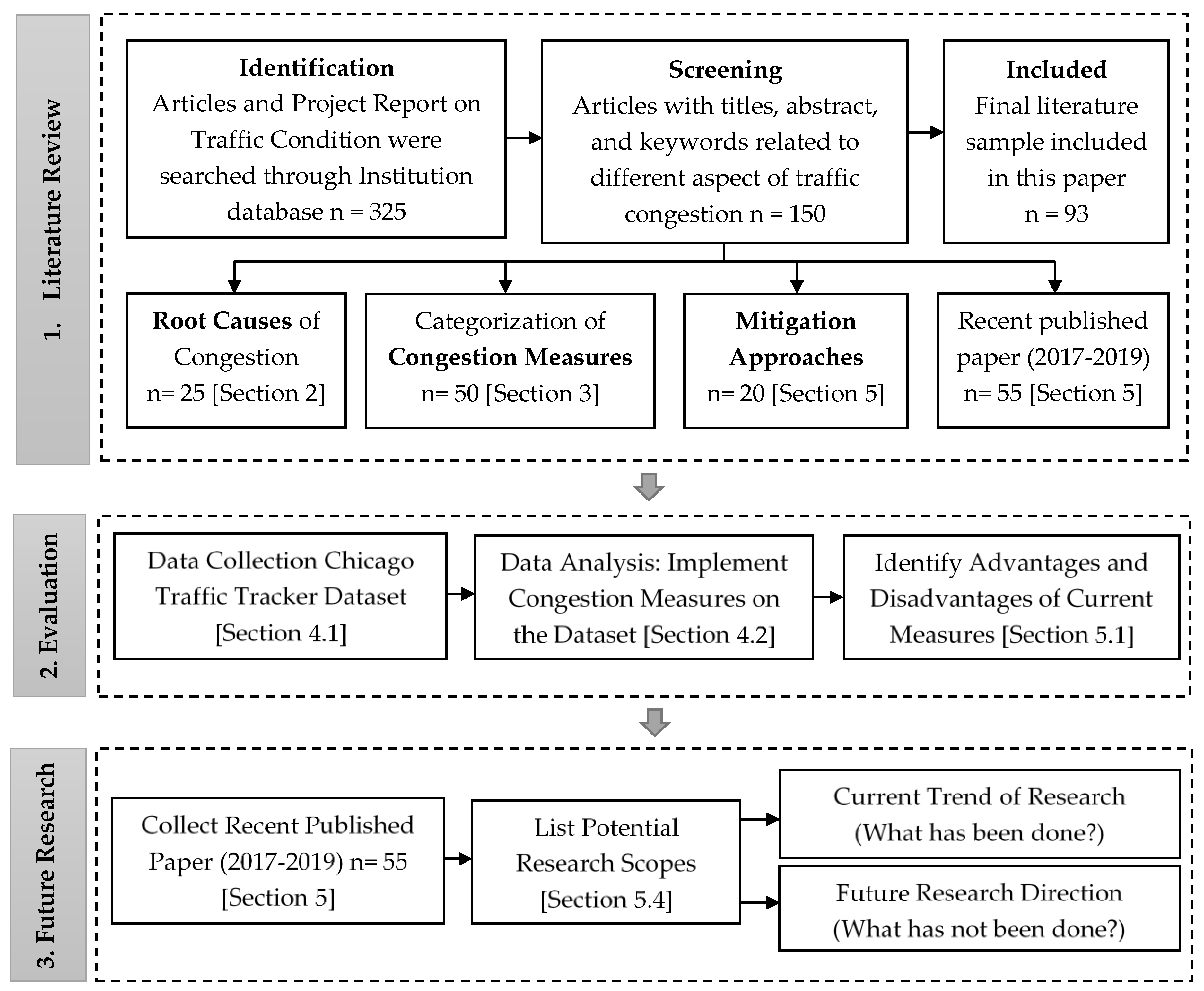
This review paper aims to elaborate on the state of the art in road traffic congestion measures as a building block towards the development of resilient and sustainable transportation system. Based on the challenges mentioned above, the motivation and objectives of this paper are as follows. (1) provide the state of the art of the currently available traffic congestion measures; (2) evaluate the effectiveness and discrepancies of the measures in monitoring traffic conditions; (3) analyze the merits and demerits of each measure; and (4) identify some prospective future research directions in the greater interest of mitigating traffic congestion towards the development of a sustainable and resilient transportation management system. Figure 1 layouts the literature review process, the evaluation, as well as the potential future direction. n denotes the number of research articles and transportation-related project reports reviewed and considered during the literature review process.

The rest of the paper is organized as follows. Section 2 illustrates the different causes of traffic congestion. Section 3 categories the currently available congestion measures and details their equations or computation methods in general. Section 4 discusses the implementation of these measures in traffic dataset and their results. Section 5 identified the advantages and disadvantages of each measure. Finally, Section 6 summarizes the key findings with the conclusion.

2. Root Causes of Congestions

Congestion in urban or metropolitan areas may occur due to various reasons, such as excess demand, signal, incidents, work zones, weather-related, or special events. Depending on various root causes, generally, road traffic congestions can be classified into two categories: (1) recurring congestions and (2) nonrecurring congestions [37].

2.1. Recurring Congestion

In most metropolitan cities, travelers experience congestion every day during daily peak hours. According to FHWA, roughly half of the congestion experienced by traffic users is recurring [5]. The common reasons for recurring congestion are:

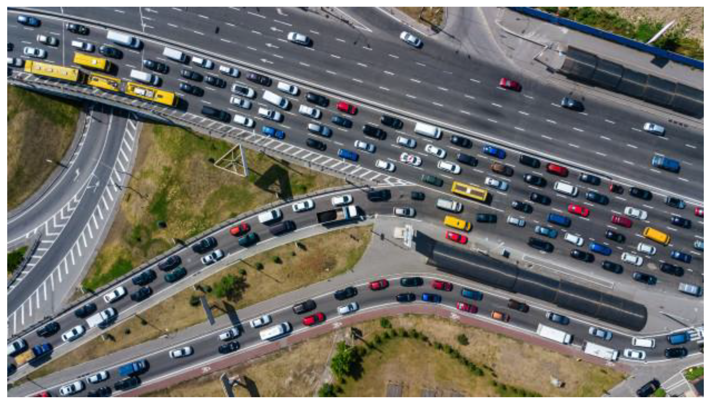
• Bottlenecks and capacity: The most common cause of congestion is due to blockages, as shown in Figure 2. Bottlenecks generally occur during peak flow hours, where the number of lanes converging on a roadway, bridge, or tunnel exceeds the number of lanes these facilities have [38,39,40]. It may also occur when the demand exceeds the capacity of a road. The capacity of any road indicates the maximum amount of traffic that can be handled. Capacity can be determined by the number and width of lanes, merging length at interchanges, and roadway alignment.

• Insufficient infrastructure: Insufficient infrastructure is one of the most significant reasons for congestion, especially in highly populated areas. Because of the higher population rate, the number of vehicles also increases with it. When the existing number of infrastructures fails to occupy this increasing number of cars, congestion occurs [42].
• Variation in traffic flow: The variability in day-to-day traffic demands results in higher volumes in some days compared to others. When these variable demands do not match with the fixed capacity, a delay may occur [37].
• Inadequate traffic controllers: Poorly timed signals or designs of traffic controllers such as traffic lights, stop signs, speed reductions, or railroad crossings can disrupt a regular traffic flow, which leads to congestion and travel time fluctuation [37].

2.2. Nonrecurring Congestions

Nonrecurring congestions generally occurred due to unpredictable events, such as traffic incidents, work zones, weather, or other particular circumstances [6,37]. Nonrecurring congestion can initiate new congestion in the off-peak periods, as well as can increase the delay due to recurring congestion. Some common examples of nonrecurring congestion are:

• Traffic incidents/accidents: The most common form of incidents is vehicular crashes, breakdowns, and debris in travel lanes. These events disrupt the normal flow of traffic, usually by blocking the travel lanes, which further results in capacity reduction [43,44].
• Work zones: Work zones refer to the construction activities on the roadway by making physical changes to the highway environment. These changes lead to a reduction in the number or width of travel lanes, lane ‘shifts’, lane diversions, reduction or elimination of shoulders, and temporary roadway closures.
• Weather: Changes in environmental conditions or weather can affect traffic flow and driver behavior. These may also modify the traffic control systems, such as signals and railway crossing, as well as road conditions. Due to bad weather induced road conditions, about 28% of all highway crashes and 19% of all fatalities take place [45]. Besides, both vehicle speed and volume can be affected by high wind-gust, heavy rains, or snow.
• Other special events: Demand variations of traffic flow about a particular event that generally differ from the usual flow pattern. These events include sports events (game day), concerts, or other social events. A sudden spike in traffic demand during special occasions can overwhelm the system and create congestion.

3. Current Approaches to Measure Congestion

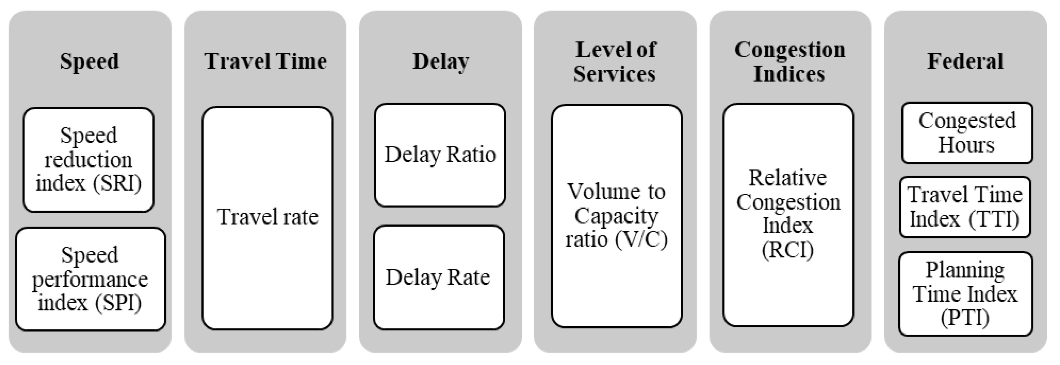
To quantify the congestion level, numerous congestion measures have been developed considering different performance criteria. Depending on these criteria, the congestion measures can be categorized into five categories: (i) speed, (ii) travel time, (iii) delay, (iv) level of services (LoS), and (v) congestion indices, as shown in Figure 3. Moreover, some measures are used by the DOT-FHWA to quantify the congestion level annually. These federal congestion measures are listed in Section 3.6. The congestion measures employed in other countries may differ from the ones discussed in this paper will be discussed briefly in Section 3.7. Note that the measures presented in this paper are not exhaustive.

3.1. Speed

3.1.1. Speed Reduction Index (SRI)

SRI is the ratio of the relative speed change between congested and free-flow conditions, as shown in Equation (1) [30,31]. The SRI ratio is multiplied by 10 to keep the value of SRI in the range of 0 to 10. Congestion occurs when the index value exceeds 4 to 5. Values less than 4 indicate a non-congested condition.

SRI = (1 − v_ac/v_ff) × 10,

(1)

where SRI denotes the speed reduction index, v_ac indicates the actual travel speed, and v_ff means the free-flow speed.

The free-flow speed generally refers to the average speed of the off-peak period. In practice, the posted speed limit can also be considered as the free-flow speed. In the FHWA’s Urban Congestion Report of 2019 [46], the 85th percentile of the off-peak speed is considered as the free-flow speed. According to the same report [46], the off-peak period is Monday through Friday, 9:00 a.m. to 4:00 p.m. and 7:00 p.m. to 10:00 p.m., and Saturday and Sunday 6:00 a.m. to 10:00 p.m.

3.1.2. Speed Performance Index (SPI)

SPI is developed to evaluate urban road traffic conditions [30]. The value of SPI (ranging from 0 to 100) can be defined by the ratio between vehicle speed and the maximum permissible speed, as shown in Equation (2). To measure the traffic state on the road with this index, the traffic state level can be classified with three threshold values (25, 50, and 75). The classification criterion of the urban road traffic state is shown in

Table 1. Speed performance index with traffic state

Speed Performance Index	Traffic State Level	Description of Traffic State
(0,25)	Heavy congestion	Low average speed, poor road traffic state
(25,50)	Mild congestion	Lower average speed, road traffic state bit weak
(50,75)	Smooth	Higher the average speed, road traffic state better
(75,100)	Very smooth	High average speed, road traffic state good

.

SPI = (v_avg/v_max) × 100,

(2)

where SPI denotes the speed performance index, v_avg indicates the average travel speed, and v_max denotes the maximum permissible road speed.

3.2. Travel Rate

Travel rate refers to the rate of motion for a particular roadway segment or trip that can be represented by the ratio of the segment travel time by the segment length [47], as shown in Equation (3). The inverse of speed can also be employed to quantify the travel rate.

Tr_r = T_t/L_s,

(3)

where, Tr_r denotes the travel rate, T_t is the travel time, and L_s indicates the segment length.

3.3. Delay

3.3.1. Delay Rate

The delay rate is the rate of time loss for vehicles operating during congestion for a specific roadway segment or trip [2,47]. It can be calculated by the difference between the actual travel rate and the acceptable travel rate as

D_r = Tr_ac – Tr_ap,

(4)

where, D_r is the delay rate, Tr_ac is the actual travel rate, and Tr_ap is the acceptable travel rate.

3.3.2. Delay Ratio

The delay ratio can be calculated by the ratio of delay rate and the actual travel rate as Equation (6). It is used to compare the relative congestion levels on different roadways [2,47].

D = D_r/Tr_ac,

(5)

where D denotes the delay ratio, D_r is the delay rate, and Tr_ac is the actual travel rate.

3.4. Level of Services (LoS)

The Highway Capacity Manual (HCM) adopts the LoS approach [48]. Because of the simplicity, LoS has become extremely popular in practice [49,50]. The LoS can be determined by various traffic quantities, such as density, speed, volume to capacity ratio, and maximum service flow rate. The LoS of a roadway can be determined by the scale intervals of the volume-to-capacity ratio (V/C), as shown in

Table 2. Level of service (LoS) based on the corresponding V/C ratio and operating conditions

LoS Class	Traffic State and Condition	V/C Ratio
A	Free flow	0–0.60
B	Stable flow with unaffected speed	0.61–0.70
C	Stable flow but speed is affected	0.71–0.80
D	High-density but the stable flow	0.81–0.90
E	Traffic volume near or at capacity level with low speed	0.91–1.00
F	Breakdown flow	>1.00

. The V/C ratio can be calculated by

V/C = N_v/N_max,

(6)

where, N_v is the spatial mean volume, and N_max denotes the maximum number of vehicles that a segment is able to contain as the capacity [49,50]. It can be further quantified as

N_max = (L_s/L_v) × N_l ,

(7)

where L_s is the spatial segment length, L_v is the average vehicle length occupancy, and N_l is the number of lanes. L_v includes vehicle length and safety distance. In general, it is assumed that vehicle length is about 14 ft. (approximately 4.27m), and safety distance is about 15 ft. (approximately 4.57m) [50].

3.5. Congestion Indices

3.5.1. Relative Congestion Index (RCI)

RCI is the ratio of delay time and free-flow travel time (T_ff) [49,50]. The RCI of 0 denotes a very low congestion level, and the values greater than two (> 2) show a significant congestion level. RCI can be calculated by

RCI = (T_ac − T_ff)/T_ff

(8)

where T_ac is the actual travel time, which is further quantified with the ratio of spatial length and spatial mean speed. The free-flow travel time (T_ff) can be calculated with the ratio of spatial length and free-flow speed.

3.5.2. Road Segment Congestion Index (R_i)

The degree of road segment congestion, denoted by R_i, can be measured by using the normal road segment state and the duration of the non-congestion state in the observation period [30]. The non-congestion state includes the traffic state where the speed performance index (SPI) is higher than 50. The R_i index value ranges between 0 and 1, and the smaller the value of R_i, the more congested the road segment is.

R_i = (SPI_avg/100) × R_NC,

(9)

R_NC = t_NC/t_t ,

(10)

where R_i is the road segment congestion index, SPI_avg is the average of the speed performance index. R_NC and t_NC denotes the proportion of non-congested state and the duration of the non-congested state, respectively. t_t is the length of the observation period.

3.6. Federal Congestion Measures

In the reports of annual urban congestion trends from 2016 to 2018, published by the DOT-FHWA, congested hours, travel time index, and planning time index were used as congestion measures. These measures are described as follows.

3.6.1. Congested Hours

The congested hours represent the average number of hours during specified periods in which road sections are crowded. Speeds less than 90% of the free-flow speed for weekdays (6:00 a.m. to 10:00 p.m.) is considered as the congested state [34,35,36,46]. For example, if most vehicles travel on a 54 mph average when the free-flow speed is 60 mph, it is considered as the congested state.

3.6.2. Travel Time Index (TTI)

TTI is proposed in the 2005 Urban Mobility Report [31,32,46]. This index is quantified by comparing travel time in the free-flow condition and the travel time in peak hours as

TTI = T_pp/T_ff = v_ff/v_pp,

(11)

where T_pp is the peak period travel time, T_ff is the free-flow travel time, v_ff is the free-flow travel speed, and v_pp is the peak period travel speed.

3.6.3. Planning Time Index (PTI)

PTI demonstrates the ratio of the 95th percentile travel time of the free-flow travel time. It is computed during the a.m. (6:00 a.m. to 9:00 a.m.) and p.m. (4:00 p.m. to 7:00 p.m.) peak periods on weekdays. A PTI of 1.60 means that travelers should anticipate an additional 60% of travel time above the free-flow travel time to ensure on-time arrival 95% of the time (or most of the time) [34,35,36,46].

3.7. Approaches in Different Countries

Different countries adopt different congestion measures to determine the congestion level. The Korea Highway Corporation (KHC) considers traffic congestion when the average vehicle speed is lesser than 19 mph for more than 2 h in a day and 10 days in a month [31]. In Japan, the speed threshold values are used to identify the congested areas. For examples, if the freeway travel speed falls below 25 mph, or there are frequent ‘stop-and-go’ flows for more than half a mile, or continues for more than 15 min, the state is called traffic congestion [31]. Since approaches in different countries are not the focus of this paper, this section is kept concise and will not be further elaborated in detail.

4. Evaluation of Current Approaches

The measures, as mentioned above, were analyzed using real-time traffic datasets to evaluate the practicality and the consistency of each measure in capturing the traffic condition. In this section, the data analysis performed for the assessment of congestion measures is described, along with the results found.

4.1. Dataset Description

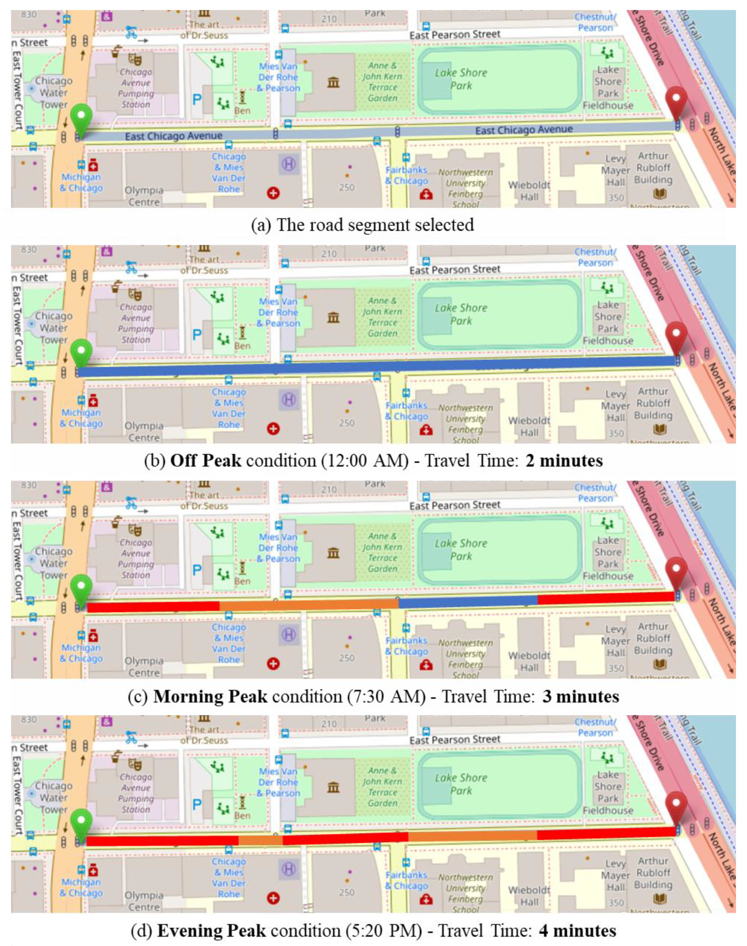
The evaluation of congestion measures was performed with an open-source dataset from the Chicago traffic tracker [51]. This dataset consists of the historical estimated congestion data for over 1,000 traffic segments, starting in approximately March 2018. Traffic congestion on Chicago’s arterial streets (non-freeway streets) in real-time can be estimated by continuously monitoring and analyzing GPS (Global Positioning System) traces received from Chicago Transit Authority (CTA) buses dataset. This dataset contains, speed, vehicle count, and segment length data for every 10 mins for seven consecutive days. For this paper, an entire week of data from 14 March 2018, to 20 March 2018, of one segment (from Michigan to Lake Shore Dr.) was considered. The specific road segment of the collected traffic data is shown in Figure 4a by using Open Street Map in both off-peak (Figure 4b) and peak hours conditions (Figure 4c,d). The traffic condition in Figure 4 was captured at the time of manuscript preparation on 18 December 2019. It is shown in Figure 4 that during an off-peak time, a driver typically needs only two minutes to travel through the road segment. However, during peak hours, a driver is estimated to need three to four minutes to travel through the road segment, depending on the congestion level.

4.2. Data Analysis

All the congestion measures from Section 3 were implemented on the described dataset to analyze both daily and weekly traffic state at different times. The data for selected daily analysis was collected on 14 March 2018, and the weekly analysis was collected from 14 March 2018, to 20 March 2018.

4.2.1. Daily Data Analysis

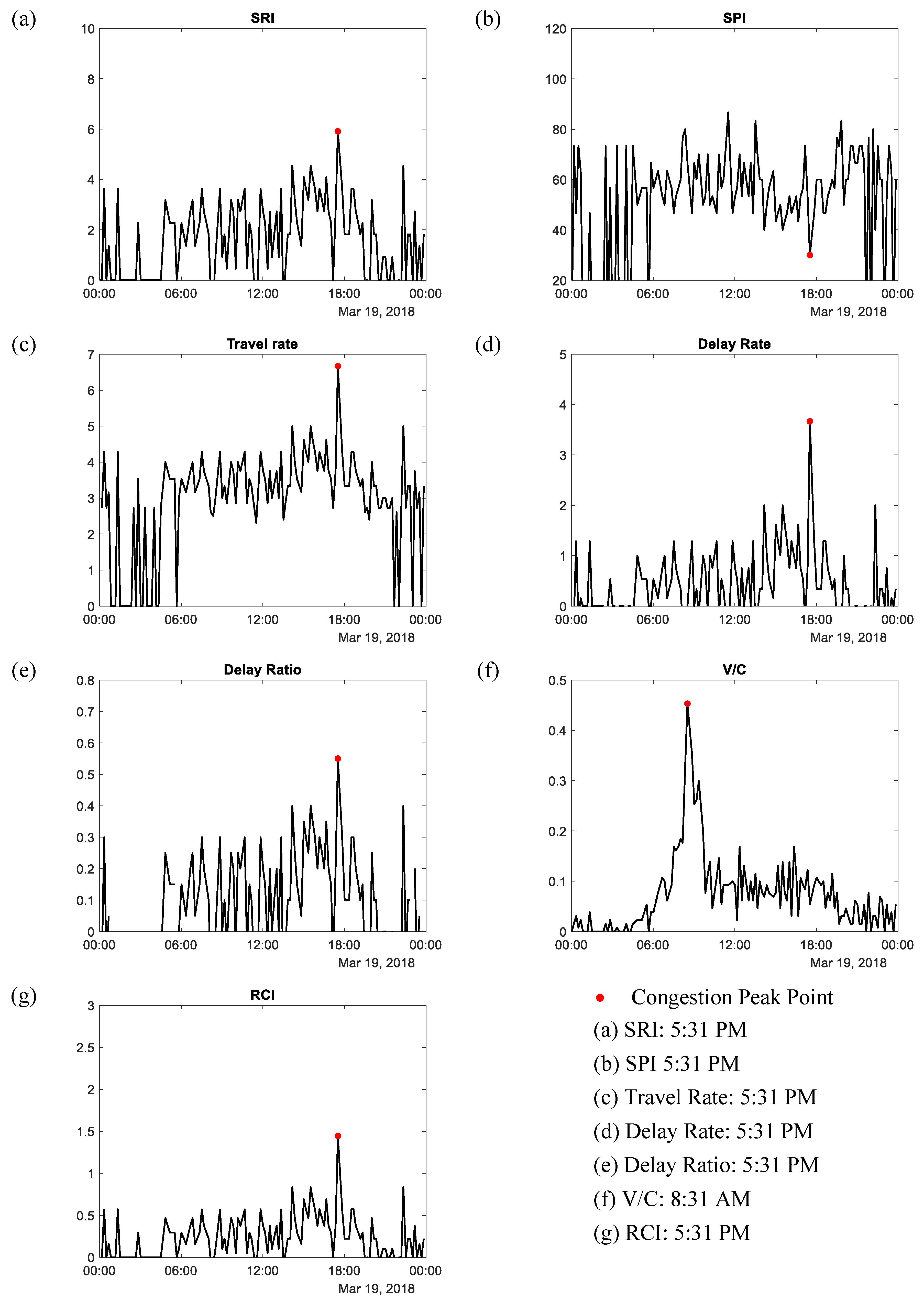
For understanding the traffic congestion at different times of a day, SRI, SPI, travel rate, delay rate, delay ratio, V/C ratio, and RCI were employed to capture traffic conditions on 19 March 2018. The behavior of each measure at different times can be found in Figure 5, where the x-axis represents the time of each day for the day, and the y-axis indicates the congestion index obtained based on different congestion measures. The y-axis in all sub-figures in Figure 5, do not have units as they represent the congestion index. As shown in Figure 5, each sub-figure has a different range of congestion index. The different range of congestion indices complicates the process of comparing various congestion measures.

For each measure, the peak points of different congestion measures for the daily data analysis are summarized in

Table 3. Peak points of different congestion measures on weekdays.

Day	Monday		Tuesday		Wednesday		Thursday		Friday
Congestion Measures	a.m.	p.m.	a.m.	p.m.	a.m.	p.m.	a.m.	p.m.	a.m.	p.m.
SRI	-	5:31	-	5:21	-	2:10	-	5:31	-	4:11
SPI	-	5:31	-	5:21	-	2:10	-	5:31	-	4:11
Travel rate	-	5:31	-	5:21	-	2:10	-	5:31	-	4:11
Delay rate	-	5:31	-	5:21	-	2:10	-	5:31	-	4:11
Delay ratio	-	5:31	-	5:21	-	2:10	-	5:31	-	4:11
V/C	8:31	-	8:51	-	-	4:50	8:50	-	8:40	-
RCI	-	5:31	-	5:21		2:10	-	5:31	-	4:11

. It can be summarized that except for the V/C ratio, all the other measures show a similar trend and the peak point at 5:31 PM. For the V/C ratio, the peak point is at 8:31 AM. In addition, it was found that based on these particular days, the road segment index value is 0.45, which indicates less congestion. The average congested hours for the day are 5 h, and the travel time index (TTI) and the planning time index (PTI) values are 1.44 and 1.08, respectively. These numbers imply that the 44% additional travel time is needed compared to free-flow travel time, and the traveler might have to plan for 8% more time while traveling through this road.

4.2.2. Weekly Data Analysis

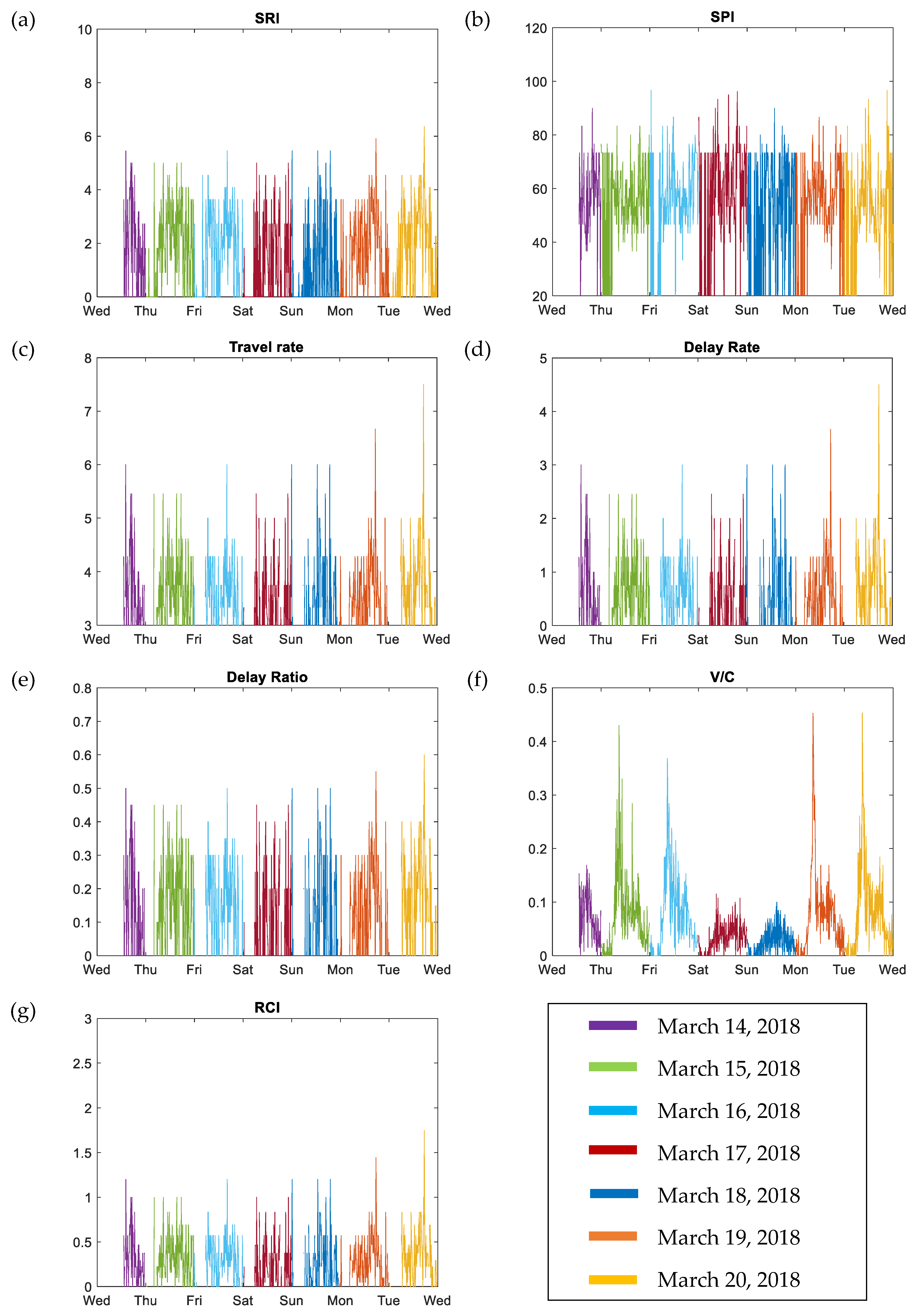
The weekly trend of the seven congestion measures is shown in Figure 6, where the x-axis represents the time of each day for an entire week, and the y-axis indicates the congestion index obtained based on different congestion measures. The y-axes in Figure 6 do not have a unit as they represent the congestion index from various congestion measures. It can be noted that each congestion measure has different ranges of congestion index. From Figure 6, it is observed that the trend of measurement values for each day is almost consistent for SRI, SPI, travel rate, delay rate, delay ratio, and RCI, except for the V/C ratio. This is because the SRI, SPI, travel rate, delay rate, delay ratio, and RCI are fundamentally calculated based on the travel speed and time. However, the V/C ratio shows a different perspective of congestion as it compares the volume of vehicles with the roadway capacity. It is also observed that the V/C ratio on Thursday, Saturday, and Sunday is significantly lower than that of the other four days.

The weekly peak point trend of these measures is also determined, which can be found in Table 3 for weekdays (Monday to Friday) and

Table 4. Peak points of different congestion measures on weekends.

Day	Saturday		Sunday
Congestion Measures	a.m.	p.m.	a.m.	p.m.
SRI	-	10:20	12:10	12:50
SPI	-	10:20	12:10	12:50
Travel rate	-	10:20	12:10	12:50
Delay rate	-	10:20	12:10	12:50
Delay ratio	-	10:20	12:10	12:50
V/C	8:50	-	-	2:40
RCI	-	10:20	12:10	12:50

for weekends (Saturday and Sunday). On weekdays Monday to Friday, congestion is observed mostly between peak hours, 6:00 a.m. to 9:00 a.m. and 4:00 p.m. to 7:00 p.m. The peak value for the most measure is found at 5:31 p.m., 5:21 p.m., 2:10 p.m., 5:31 p.m., and at 4:11 p.m. on Monday, Tuesday, Wednesday, Thursday, and Friday, respectively. However, the peak value is found to be different at weekends at 12:10 a.m. and 12:50 p.m. on Sunday, and 10:20 p.m. on Saturday.

When analyzing the congestion trend, a different type of trend is observed for the V/C ratio if compared to other measures. For the weekdays, on Monday, Tuesday, Wednesday, Thursday, and Friday, the peak point is at 8:31 a.m., 8:51 a.m., 4:50 p.m., 8:50 a.m., and 8:40 a.m., respectively. Further, on the weekends, the peak point based on the V/C ratio is observed at 8:50 a.m. on Saturday and at 2:40 p.m. on Sunday. The variation in congestion during weekdays and weekends could occur because of the high rate of flow and volume of vehicles on the road on weekdays, which is not typically observed on the weekends.

While measuring congestion with different measures, sometimes negative values may occur for delay rate and delay ratio. This is because the difference between the actual and acceptable travel time can be negative when the actual travel time is less than the acceptable travel time. It typically happens especially at midnight, when fewer vehicles are traveling, and the average vehicle speed is quite high. During this time, no congestion occurs as most cars take lesser time than average travel time. In all the subfigures, the value of zero does not indicate if there is no congestion. Instead, it means that there is no vehicle on the road. From this analysis, it is observed that different congestion measures may have a different numerical value, but they also indicate a consistent congestion level within the range of each measure.

Assuming the daily and weekly data used in the data analysis is the typical (recurring) congestions, the monthly and yearly recurring congestion trend may be similar to the weekly congestion trend in Figure 6. Slight variations of recurring congestions behavior from week to week in a year are expected due to variations in traffic flow, weather conditions, and season changes. In addition, nonrecurring congestions are expected in some days or weeks as well. However, to analyze the nonrecurring condition, additional information on nonrecurring congestions events is required.

4.2.3. Case Study Discussion

Different congestion measures may have an impact on a decision, for example, whether the current traffic condition should be classified as congested or not, and how bad the congestion level is. From all the seven measures employed in data analysis, some of the discussed measures have a cutoff value for the congestion state, for example, SRI indicates a congestion state when its value exceeds 4 to 5, and for RCI, the congestion state starts from 2. Apart from the congestion state, some measures offer a range of value to different levels of congestions. The SPI and V/C measures provide a set of values to indicate various levels of congestion, as shown in Table 1 and Table 2, respectively. The range of value is often useful in a detailed daily congestion analysis.

Comparing SRI that has a range of 0–10 and SPI that has a scale of 0–100,

Table 5. Congestion on each day of a week based on SRI and SPI

Day		SRI	Count	SPI	Count
Sunday	a.m.	12:10, 8:20	2	12:10, 6:40, 8:01, 8:20, 11:20	5
	p.m.	7:31, 7:01, 4:50, 2:31, 2:10, 1:40, 12:50	7	12:50,1:40, 2:10–2:31, 3:31, 4:01, 4:31, 4:50, 5:40, 7:01, 7:31, 9:40	11
Monday	a.m.	-		12:20, 1:20, 7:31, 4:51, 10:40, 11:50	6
	p.m.	2:10, 3:01, 3:40, 4:40, 5:31, 10:20	6	1:21, 2:10, 3:01–4:10, 4:40, 5:31–5:50, 6:31–6:40, 10:20	7
Tuesday	a.m.	6:21,7:21, 10:50	3	6:01, 6:21, 7:10,7:21, 7:40, 7:51, 10:50, 11:01	8
	p.m.	12:31, 2:31, 2:50, 3:31–3:50, 5:01–5:31, 7:50	6	12:31, 1:10, 2:31, 3:01, 3:31–4:01, 5:01–5:31, 6:10, 7:50, 8:01, 8:20, 8:40, 11:50	12
Wednesday	a.m.	-		-
	p.m.	2:10, 4:01–4:40, 5:10, 5:40, 6:31	5	1:10, 2:10–2:21, 3:01, 4:01–4:40, 5:10, 5:21, 5:40, 6:31	8
Thursday	a.m.	4:10, 8:31–8:40, 10:50, 11:01, 11:40	5	7:31, 7:40, 8:31, 8:40, 10:01, 10:50, 11:01, 11:40	8
	p.m.	1:01, 3:10–3:21, 4:31, 5:31, 6:10, 7:50, 9:01	7	12:21, 1:01, 1:40, 3:10, 3:21, 3:50, 4:31, 5:10, 5:31, 5:50–6:10, 7:50, 9:01, 9:10	13
Friday	a.m.	4:01, 6:40–6:50	2	5:40, 6:40, 6:50, 7:21, 7:51, 8:11, 9:01, 9:21, 10:10	9
	p.m.	3:01, 3:30, 4:11, 6:50, 7:50	5	12:01, 2:31, 3:01, 3:30, 4:11, 5:30, 5:40, 6:40, 6:50, 7:50, 9:20, 11:40	12
Saturday	a.m.	6:40, 8:01, 11:01,11:10	4	5:20, 6:40, 8:01, 10:20, 11:01, 11:10 11:40	7
	p.m.	3:10, 3:40, 6:10, 9:01, 10:20	5	2:01, 3:10, 3:40, 5:31, 6:10, 9:01, 10:20, 11:31	8
Total Count		SRI	57	SPI	114

summarized the congested conditions and congestion counts found at different times for each day in a whole week. It can be seen that SPI shows more congested points compared to SRI, although some of these time instants are similar. The reason may be the range of values for SPI is more significant than that of SRI. Thus, SPI shows more instances of the congested period in a day or a week compared to the SRI measure. Based on the data analysis, SPI shows a total of 114 counts of congestion incidents, while SRI showed a total of 57 congestion incidents in a week.

While SPI and SRI may indicate congestion incidents and counts in a period, there are other measures, such as V/C and RCI, that do not indicate any congested period. For RCI, the cutoff value for the congested state is 2, which is not found in Figure 6. Similarly, all values of V/C are less than 0.5, which indicates the normal traffic state. With these measures, the information on the congestion count cannot be directly measured or obtained.

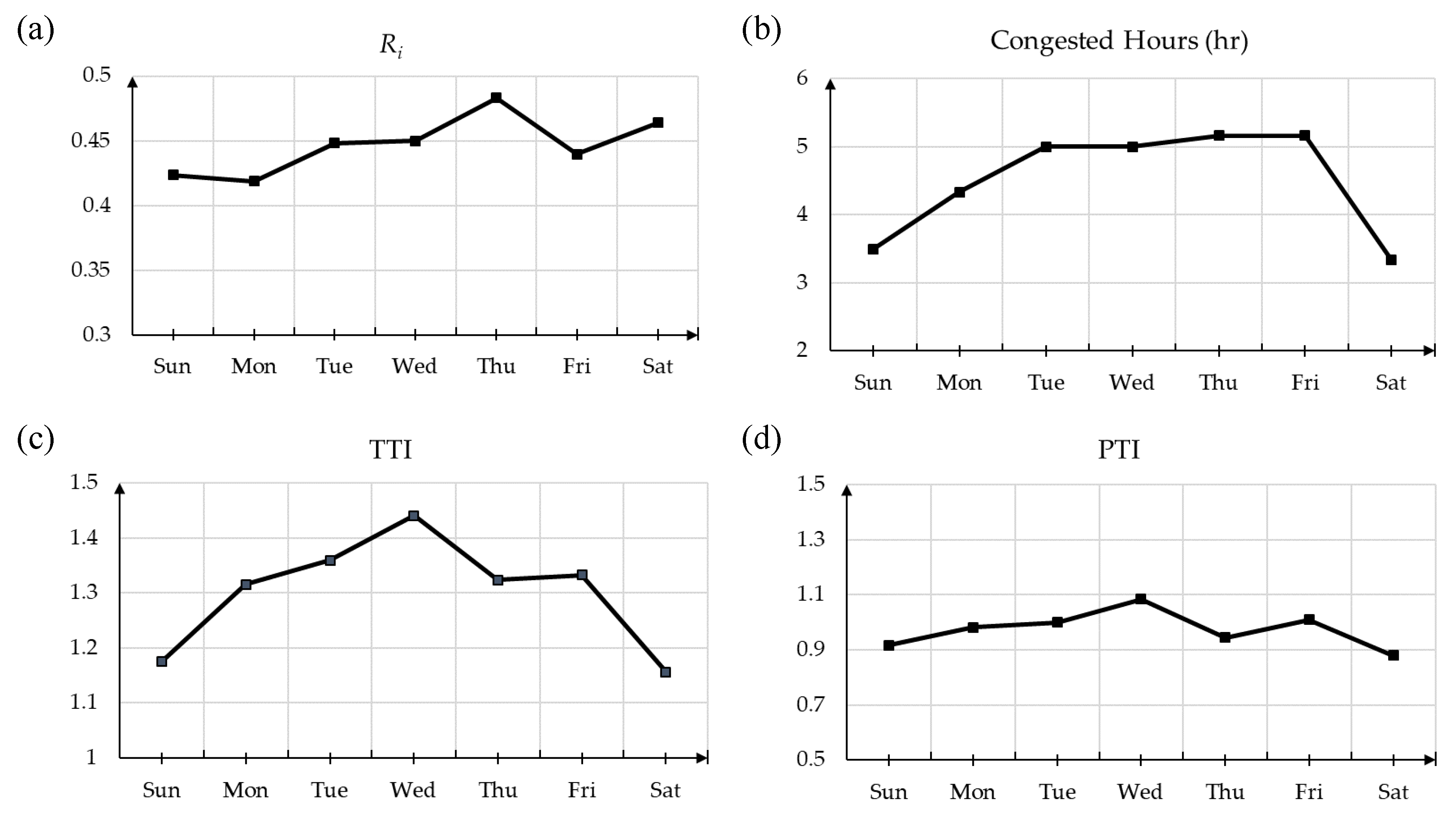
Travel rate, delay rate, relay ratio, road segment index (R_i), and the federal measures do not explicitly provide a range of value, but only a point value, for congested traffic conditions. Nonetheless, the point value may also be handy when comparing daily, weekly, or monthly traffic conditions. The comparison of the road segment congestion index (R_i) and the three federal measures (congested hours, travel time index (TTI), and planning time index (PTI)) for the entire week can be found in

Table 6. Road segment index (R_i) and federal measures

Day	Ri	Congested Hours	TTI	PTI
Sunday	0.42	3.5	1.17	0.91
Monday	0.41	4.3	1.31	0.98
Tuesday	0.44	5	1.35	1
Wednesday	0.45	5	1.44	1.08
Thursday	0.48	5.16	1.32	0.94
Friday	0.44	5.16	1.33	1.01
Saturday	0.46	3.33	1.15	0.88

and Figure 7. In Figure 7, the x-axis represents the time of each day for a total week, and the y-axis indicates the congestion index. The y-axes in Figure 7 do not have units, as each of the y-axis in each sub-figure represents the congestion index. Similar to Figure 5 and Figure 6, all of these measures in Figure 7 also show a higher value for weekdays than weekends, which further indicate a comparatively higher congestion level on the weekdays compared to the weekends.

5. Discussion

In this section, further discussion on the characteristics of each congestion measures based on the data analysis conducted is deliberated. From the analysis of the attributes of the currently available congestion measures, the criteria of a good congestion measure are also described. At the end of the section, some of the potential future research scopes towards a sustainable and resilient transportation management system are identified.

5.1. Advantages and Disadvantages of Congestion Measures

The characteristics of the currently available congestion measures were analyzed based on the found results from the data analysis of Section 4. The deviation of the current performance from the non-congested performance can be easily comprehensible from these measures. Additionally, it should be noted that the applicability of the measures differs from each other. For instance, speed-related measures and travel time index are less suitable for nonrecurring congestion scenarios. The advantages and disadvantages of various measures discussed in the data analysis section are compiled in

Table 7. Advantages and disadvantages of various congestion measures [2,32,52,53,54].

Category	Measurement Approach	Congestion Range	Advantages	Disadvantages
Speed	Speed reduction index (SRI)	>4	Easily comprehensible Provides information about relative vehicle speed in normal and congested condition	Does not consider nonrecurring conditions
	Speed performance index (SPI)	Different range levels
Travel time	Travel rate	No range available	Both time and space are accounted for	Capacity is not included
Delay	Delay rate	No range available	Can be used to estimate system performance and choose efficient travel method	Limited for a specific road type No suggested congestion range
	Delay ratio	No range available	Compares relative congestion levels in different types of roads
Level of services (LoS)	Volume to capacity ratio	Different range levels	Comprehensible by non-technical users	Cannot provide continuous congestion value No information on speed and time are considered
Congestion indices	Relative congestion index (RCI)	>2	Spatial-mean performance of traffic is represented	Limited to particular road type
	Road segment congestion index	No range available	Appropriate to represent segment condition	Only applicable to measure specific segment conditions.
Federal	Congested Hours	No range available	Provides an estimation of the congested time period	Only depends on the speed
	Travel time index (TTI)	No range available	Accounts for recurring congestion Both time and space are considered	Value could vary due to different peak period consideration
	Planning time index (PTI)	No range available	Describes travel time reliability to planners as well as network users	Planning for additional travel time might not always be reliable

.

5.2. Criteria of a Good Congestion Measure

Measuring the congestion level is crucial for improving traffic management and control. The following decision-making steps towards a sustainable transportation system are highly dependent on the actual road traffic conditions. Thus, the measurement approach to quantify the congestion severity should be practical enough for the decision-makers to implement necessary steps to mitigate congestion promptly to achieve a sustainable and resilient transportation system. Transportation experts have suggested a range of attributes that are often desired in a congestion measure [2,53,55,56,57]; a good congestion measure should:

• be well-defined, easily comprehensible, and uncomplicated for non-technical users to interpret the results easily,
• reflect the real level of service for any road types,
• consider different system performances, such as travel time and speed,
• provide a continuous range of values,
• be able to be used in predictive and statistical analysis purposes,
• offer comparable values to different road types, and
• be widely applicable for different road types

5.3. Current Mitigation Approaches

Traffic congestion has always been a constant global challenge. Although there is no guarantee that congestion can be entirely dismissed due to the growing global population, transportation experts from different countries have been working on mitigating congestion to a great extent [3,58,59,60]. Most of the implemented mitigation approaches, such as effective transportation management plans (TMPs) developed by the DOT, are successful in reducing the percentage of congestion for a while. Some of the most applied congestion mitigation approaches for both recurring and nonrecurring congestion are:

• Add more base capacity. The capacity of road infrastructure can be improved by increasing the number and size of highways, providing more transit and freight rail service, adding additional lanes, and building new highways [3,58,59,60]. However, this approach typically demands a substantial amount of implementation costs.
• Operate the existing infrastructures efficiently. The existing infrastructures can be utilized more efficiently by redesigning mitigation routes for specific bottlenecks, such as in the interchanges and intersections, to increase their function or their baseline capacity [3].
• Various-sector traffic management. For incident management, identifying accidents quickly, improving response times, and managing accidents or other incident scenes more effectively can help in reducing the event induced congestions [44,61]. For the work zone, managing traffic in a work zone area is necessary to reduce congestion, particularly at peak hours. Thus, the work zone should be planned cautiously [62,63]. Planning for special events ahead of time and coordinate with the traffic control plans may ease congestion [6,64]. Controlling traffic signals, ramp meters, and manage lane usage with a computerized system are often found to a practical approach in reducing congestion during peak hours [3]. Different management protocols, such as travel demand management (TDM), non-automotive travel modes, and land use management, can be followed [65].
• Weather and traveler information. Predicting weather conditions in specific areas and roadways would be beneficial for travelers to be prepared for congestions [66,67]. Suggesting alternative routes for travelers ahead of the congestion period and area may reduce the volume-to-capacity ratio in the congestion area [3].
  Value pricing strategies. The dynamicity of traffic demand can be adjusted with the capacity by imposing tolls [3,58]. This strategy may discourage travelers from traveling during the congestion period.

5.4. Potential Future Research Directions

From the analysis of different congestion measures, it is evident that there are considerable scopes for improvement in this field towards the development of a sustainable and resilient transportation system. Some of the potential future research scopes to reduce congestion, improve resilience, and ensure sustainability towards a more outstanding urban transportation system are discussed as follows. Please note that the research directions are not exhaustive and may require multi-disciplinary research approaches.

• Resilient traffic management system. Resilient often defines as how fast an entity can recover from its disrupted states [68,69,70]. Since the recurring congestion is a cyclical scenario, the analysis of how quickly traffic congestion can return to its normal operating state without congestion will be beneficial in developing a resilient transportation management system [49,50,71]. Additionally, a resilience-based congestion measure for both recurring and nonrecurring congestions is an area that has a potential research scope. Several resilience-oriented congestion measures have been proposed for recurring congestion [49,50]. However, resilience-based measures for nonrecurring congestion is still underexplored.
• Analysis of nonrecurring congestion. A sustainable and resilient transportation system should be able to offer interrupted functionality during unexpected events. Due to the increased intensity and frequency of the natural-related disasters, nonrecurring congestion is a field of study that should be explored extensively in terms of measurement approach, predictive analysis, and uncertainty investigation [7,15,72,73,74]. The probability of occurring congestion varies for different types of events, where some events are completely unpredictable, such as incidents from vehicles crashes unexpected weather changes, and evacuation due to disasters [7,8,75,76].
  The pattern and probability occurrence of the root cause events for nonrecurring congestion are often uncertain. Thus, it is relatively difficult to control and manage the traffic accurately while the event is happening [21]. Especially during disasters, when an evacuation is needed, traffic congestion is commonly encountered, which excessively slows down the evacuation process. Several efforts have been made to analyze the impact of congestion on evacuation and increase efficiency can be found in Refs. [8,43,77]. The pattern detection methods for nonrecurring congestion during evacuation for predictive analysis can be investigated further to reduce evacuation-related congestion.
• Smart traffic management system. The development of a sustainable and resilient transportation system may be achieved with the aid of technological advancements. As computational technologies advance rapidly, the conventional traffic management systems have evolved to become more intelligent with the help of IoT (Internet of Things). IoT-based traffic management systems and congestion mitigation techniques are often developed for smart urban areas [27,78,79]. Different data-driven approaches are employed to predict the time, probability, and the level of congestion [29,80,81,82]. However, congestion can still occur in many cases due to the deviation of prediction with implementation, or the improper usage of predicted features. In the future, these issues should be addressed.
  The research on smart traffic management can also be leveraged to include the nonrecurring congestion scenario, for example, in predicting the most effective time of implementing evacuation or other mitigation approaches [8,77]. In addition to smart traffic management systems, the retrofit process of current infrastructures, for example, to accommodate the rapidly increasing charging stations and electric vehicles on roads, is another prospective future research area towards the development of a sustainable transportation system [83].
• Social-environmental effects of congestion. The irreversible environmental impacts on congestion are constantly increasing day-by-day. Different advanced sustainability approaches have been developed to reduce fuel consumption and greenhouse gas emission due to congestion [25,84,85]. Various strategies that fall under the intelligent transport system (ITS) categories, such as adaptive traffic light control systems [86,87], have been proposed but sparsely implemented. The impacts of such methods are believed to be able to reduce the negative environmental effects as well as provide pollution-free air by reducing congestion significantly. Over recent years, electric vehicles have become a popular potential option to combat carbon emissions. However, there are also other environmental impacts imposed by batteries from electric vehicles [88,89]. Thus, proper recycling procedures should be researched further [90,91,92].
• Socioeconomic effects of congestion. Traffic congestion significantly affects urban life from both social and economic aspects [9,93]. The causes and consequences of urban traffic congestion have been considerably explored [13]. The overall productivity of society reduces due to traffic congestion, which, in result, affects the economy as well [13,58]. The socioeconomic aspects should be incorporated in the congestion mitigation research so that the negative socioeconomic impacts of congestion can be reduced.

6. Conclusions

Traffic congestion is a global challenge in the development of sustainable and resilient traffic management systems. In this paper, an overview of the causes of road traffic congestion is presented for both recurring and nonrecurring congestion. In addition to this, the currently available traffic congestion measures are categorized into seven different categories: (i) speed, (ii) travel time, (iii) delay, (iv) level of services (LoS), (v) congestion indices, (vi) federal approaches, and (vii) a brief discussion on the strategies employed in different countries. For each category, congestion measures are described with their corresponding equations and quantitative ranges for various congestion levels. A real-time traffic tracker dataset was used to compare seven congestion measures. Daily and weekly analysis of congestion were performed for a road segment. From the daily analysis, a similar peak congestion period was observed for different congestion measures. Additionally, the weekly analysis showed a slight difference of peak congestion period from day-to-day. Moreover, the advantages and disadvantages of each measure are identified, along with the criteria of a good congestion measure.

Although there is no guarantee that traffic congestion can be resolved entirely, some of the widely used mitigation approaches are listed in this study. Considering the available measurement and mitigation approaches, a wide variety of potential future research directions were discussed. This review paper mainly consists of non-probabilistic congestion measures. For immediate future work, various probabilistic congestion measures will be evaluated as they are more appropriate to be employed in congestion prediction and mitigation plans. In addition, more in-depth data analysis will be conducted by considering various locations (or road segments), different traffic conditions, and the complexity of the road structures. Overall, this study determines current challenges in traffic congestion measurement approaches and provides a new insight towards the development of a sustainable and resilient traffic management system in the long run.

References

- Reed, T.; Kidd, J. Global Traffic Scorecard; INRIX Research: Altrincham, UK, 2019. [Google Scholar]
- Aftabuzzaman, M. Measuring traffic congestion—A critical review. In Proceedings of the 30th Australasian Transport Research Forum (ATRF), Melbourne, Australia, 25–27 September 2007. [Google Scholar]
- Systematics, C. Traffic Congestion and Reliability: Trends and Advanced Strategies for Congestion Mitigation; Cambridge Systematics Inc.: Cambridge, MA, USA, 2005. [Google Scholar]
- Litman, T. Congestion Reduction Strategies: Identifying and Evaluating Strategies to Reduce Traffic Congestion; Victoria Transport Policy Institute: Victoria, BC, Canada, 2007. [Google Scholar]
- FHWA. Operations–Reducing Recurring Congestion. Available online: https://ops.fhwa.dot.gov/program_areas/reduce-recur-cong.htm (accessed on 10 December 2019).
- Falcocchio, J.C.; Levinson, H.S. Managing nonrecurring congestion. In Road Traffic Congestion: A Concise Guide; Springer: Berlin/Heidelberg, Germany, 2015; pp. 197–211. [Google Scholar]
- Ghosh, B. Predicting the Duration and Impact of the Nonrecurring Road Incidents on the Transportation Network. Ph.D. Thesis, Nanyang Technological University, Singapore, May 2019. [Google Scholar]
- Fonseca, D.J.; Moynihan, G.P.; Fernandes, H. The role of nonrecurring congestion in massive hurricane evacuation events. In Recent Hurricane Research—Climate, Dynamics, and Societal Impacts; InTech: London, UK, 2011; pp. 441–458. [Google Scholar]
- Tonne, C.; Beevers, S.; Armstrong, B.; Kelly, F.; Wilkinson, P. Air pollution and mortality benefits of the London Congestion Charge: Spatial and socioeconomic inequalities. Occup. Environ. Med. 2008, 65, 620–627. [Google Scholar] [CrossRef]
- Armah, F.A.; Yawson, D.O.; Pappoe, A.A. A systems dynamics approach to explore traffic congestion and air pollution link in the city of Accra, Ghana. Sustainability 2010, 2, 252–265. [Google Scholar] [CrossRef] [Green Version]
- Wang, J.; Chi, L.; Hu, X.; Zhou, H. Urban traffic congestion pricing model with the consideration of carbon emissions cost. Sustainability 2014, 6, 676–691. [Google Scholar] [CrossRef] [Green Version]
- Liu, Y.; Yan, X.; Wang, Y.; Yang, Z.; Wu, J. Grid mapping for spatial pattern analyses of recurrent urban traffic congestion based on taxi GPS sensing data. Sustainability 2017, 9, 533. [Google Scholar] [CrossRef] [Green Version]
- Bull, A.; Thomson, I. Urban traffic congestion: Its economic and social causes and consequences. Cepal Rev. 2002, 72, 1–12. [Google Scholar]
- Schrank, D.; Eisele, B.; Lomax, T.; Bak, J. Urban Mobility Scorecard; Transportation Research Board: Washingtopn, DC, USA, 2015. [Google Scholar]
- Dubey, A.; White, J. Dxnat-deep neural networks for explaining nonrecurring traffic congestion. arXiv 2018, arXiv:1802.00002. [Google Scholar]
- Pishue, B. U.S. Traffic Hot Spots: Measuring the Impact of Congestion in the United States; National Academies of Sciences, Engineering, and Medicine: Washington, DC, USA, 2017. [Google Scholar]
- Traffic Congestion Cost the U.S. Economy Nearly $87 Billion in 2018. Available online: https://www.weforum.org/agenda/2019/03/traffic-congestion-cost-the-us-economy-nearly-87-billion-in-2018 (accessed on 12 December 2019).
- Harris, N.; Shealy, T.; Klotz, L. Choice architecture as a way to encourage a whole systems design perspective for more sustainable infrastructure. Sustainability 2017, 9, 54. [Google Scholar] [CrossRef] [Green Version]
- Little, R.G. Controlling cascading failure: Understanding the vulnerabilities of interconnected infrastructures. J. Urban Technol. 2002, 9, 109–123. [Google Scholar] [CrossRef]
- Afrin, T.; Yodo, N. Resilience-Based Recovery Assessments of Networked Infrastructure Systems under Localized Attacks. Infrastructures 2019, 4, 11. [Google Scholar] [CrossRef] [Green Version]
- Yodo, N.; Wang, P.; Rafi, M. Enabling resilience of complex engineered systems using control theory. IEEE Trans. Reliab. 2018, 67, 53–65. [Google Scholar] [CrossRef]
- Bhandari, A.; Patel, V.; Patel, M.A. Survey on Traffic Congestion Detection and Rerouting Strategies. In Proceedings of the 2nd International Conference on Trends in Electronics and Informatics (ICOEI), Tirunelveli, India, 11–12 May 2018. [Google Scholar]
- Li, Z.; Liu, P.; Xu, C.; Duan, H.; Wang, W. Reinforcement learning-based variable speed limit control strategy to reduce traffic congestion at freeway recurrent bottlenecks. IEEE Trans. Intell. Transp. Syst. 2017, 18, 3204–3217. [Google Scholar] [CrossRef]
- Stefanello, F.; Buriol, L.S.; Hirsch, M.J.; Pardalos, P.M.; Querido, T.; Resende, M.G.; Ritt, M. On the minimization of traffic congestion in road networks with tolls. Annal. Oper. Res. 2017, 249, 119–139. [Google Scholar] [CrossRef]
- Choudhary, A.; Gokhale, S. Evaluation of emission reduction benefits of traffic flow management and technology upgrade in a congested urban traffic corridor. Clean Technol. Environ. Policy 2019, 21, 257–273. [Google Scholar] [CrossRef]
- Nellore, K.; Hancke, G.P. A survey on urban traffic management system using wireless sensor networks. Sensors 2016, 16, 157. [Google Scholar] [CrossRef] [Green Version]
- Kumar, T.; Kushwaha, D.S. An approach for traffic congestion detection and traffic control system. In Information and Communication Technology for Competitive Strategies; Springer: Berlin/Heidelberg, Germany, 2019; pp. 99–108. [Google Scholar]
- Cárdenas-Benítez, N.; Aquino-Santos, R.; Magaña-Espinoza, P.; Aguilar-Velazco, J.; Edwards-Block, A. Medina Cass A. Traffic congestion detection system through connected vehicles and big data. Sensors 2016, 16, 599. [Google Scholar]
- Feng, X.; Saito, M.; Liu, Y. Improve urban passenger transport management by rationally forecasting traffic congestion probability. Int. J. Prod. Res. 2016, 54, 3465–3474. [Google Scholar] [CrossRef]
- He, F.; Yan, X.; Liu, Y.; Ma, L. A traffic congestion assessment method for urban road networks based on speed performance index. Procedia Eng. 2016, 137, 425–433. [Google Scholar] [CrossRef] [Green Version]
- Rao, A.M.; Rao, K.R. Measuring urban traffic congestion—A review. Int. J. Traffic Trans. Eng. 2012, 2, 4. [Google Scholar]
- Lomax, T.J.; Schrank, D.L. The 2005 Urban Mobility Report; Texas A & M Transportation Institution: College Station, TX, USA, 2005. [Google Scholar]
- Bar-Gera, H. Evaluation of a cellular phone-based system for measurements of traffic speeds and travel times: A case study from Israel. Trans. Res. Part C Emerg. Technol. 2007, 15, 380–391. [Google Scholar] [CrossRef]
- U.S. Department of Transportation—Federal Highway Administration. 2016 Urban Congestion Trends; Federal Highway Administration: Washington, DC, USA, 2016.
- U.S. Department of Transportation—Federal Highway Administration. 2017 Urban Congestion Trends; Federal Highway Administration: Washington, DC, USA, 2017.
- U.S. Department of Transportation—Federal Highway Administration. 2018 Urban Congestion Trends; Federal Highway Administration: Washington, DC, USA, 2018.
- Falcocchio, J.C.; Levinson, H.S. Road Traffic Congestion: A Concise Guide; Springer: Berlin/Heidelberg, Germany, 2015; Volume 7. [Google Scholar]
- Suresh, S.; Whitt, W. The heavy-traffic bottleneck phenomenon in open queueing networks. Oper. Res. Lett. 1990, 9, 355–362. [Google Scholar] [CrossRef]
- Cassidy, M.J.; Bertini, R.L. Some traffic features at freeway bottlenecks. Transp. Res. Part B Methodol. 1999, 33, 25–42. [Google Scholar] [CrossRef] [Green Version]
- Laval, J.A.; Daganzo, C.F. Lane-changing in traffic streams. Transp. Res. Part B Methodol. 2006, 40, 251–264. [Google Scholar] [CrossRef]
- Highway Bottleneck Blues: 3PL Cleveland Trucking Solutions to Cut Costs—On Time Delivery & Warehouse. 2019. Available online: https://otdw.net/2019/05/25/highway-bottleneck-blues-3pl-cleveland-trucking-solutions-to-cut-costs/ (accessed on 14 December 2019).
- Wang, Y.; Zhu, X.; Li, L.; Wu, B. Reasons and countermeasures of traffic congestion under urban land redevelopment. Procedia Soc. Behav. Sci. 2013, 96, 2164–2172. [Google Scholar] [CrossRef] [Green Version]
- Robinson, R.M.; Collins, A.J.; Jordan, C.A.; Foytik, P.; Khattak, A.J. Modeling the impact of traffic incidents during hurricane evacuations using a large scale microsimulation. Int. J. Disaster Risk Reduct. 2018, 31, 1159–1165. [Google Scholar] [CrossRef]
- Haselkorn, M.; Yancey, S.; Savelli, S. Coordinated Traffic Incident and Congestion Management (TIM-CM): Mitigating Regional Impacts of Major Traffic Incidents in the Seattle I-5 Corridor; Deptartment of Transportation. Office of Research and Library: Washington, DC, USA, 2018.
- Mahmassani, H.S.; Dong, J.; Kim, J.; Chen, R.B.; Park, B.B. Incorporating Weather Impacts in Traffic Estimation and Prediction Systems; Joint Program Office for Intelligent Transportation Systems: Washington, DC, USA, 2009. [Google Scholar]
- Documentation and Definitions—Urban Congestion Reports—Operations Performance Measurement—FHWA Operations. Available online: https://ops.fhwa.dot.gov/perf_measurement/ucr/documentation.htm (accessed on 15 December 2019).
- Ter Huurne, D.; Andersen, J. A Quantitative Measure of Congestion in Stellenbosch Using Probe Data. In Proceedings of the first International Conference on the use of Mobile Informations and Communication Technology (ICT) in Africa UMICTA 2014, Stellenbosch, South Africa, 9–10 December 2014; ISBN 978-0-7972-1533-7. [Google Scholar]
- Manual, H.C. Transportation Research Board Special Report 209; Transportation Research Board: Washington, DC, USA, 1994. [Google Scholar]
- Wan, C.; Yang, Z.; Zhang, D.; Yan, X.; Fan, S. Resilience in transportation systems: A systematic review and future directions. Transp. Rev. 2018, 38, 479–498. [Google Scholar] [CrossRef]
- Tang, J.; Heinimann, H.R. A resilience-oriented approach for quantitatively assessing recurrent spatial-temporal congestion on urban roads. PLoS ONE 2018, 13, e0190616. [Google Scholar] [CrossRef] [Green Version]
- Chicago Traffic Tracker—Historical Congestion Estimates by Segment—2018-Current—Data.gov.s. Available online: https://catalog.data.gov/dataset/chicago-traffic-tracker-historical-congestion-estimates-by-segment-2018-current (accessed on 10 October 2019).
- Hamad, K.; Kikuchi, S. Developing a measure of traffic congestion: Fuzzy inference approach. Transp. Res. Rec. 2002, 1802, 77–85. [Google Scholar] [CrossRef]
- Lomax, T.J. Quantifying Congestion; Transportation Research Board: Washington, DC, USA, 1997. [Google Scholar]
- Byrne, G.; Mulhall, S. Congestion Management: Data Requirements and Comparisons in the Development of Measures for A Multimodal Congestion Management System. In Proceedings of the Fifth National Conference on Transportation Planning Methods Applications—Volume I: A Compendium of Papers Based on a Conference, Seattle, DC, USA, 17–21 April 1995. [Google Scholar]
- Turner, S.M.; Lomax, T.J.; Levinson, H.S. Measuring and Estimating Congestion Using Travel Time–Based Procedures. Transp. Res. Rec. 1996, 1564, 11–19. [Google Scholar] [CrossRef]
- Boarnet, M.G.; Kim, E.J.; Parkany, E. Measuring traffic congestion. Transp. Res. Rec. 1998, 1634, 93–99. [Google Scholar] [CrossRef]
- Lomax, T.; Turner, S.; Shunk, G.; Levinson, H.S.; Pratt, R.H.; Bay, P.N.; Douglas, G.B. Quantifying Congestion. Volume 2: User’s Guide; Transportation Research Board: Washington, DC, USA, 1997. [Google Scholar]
- Triantis, K.; Sarangi, S.; Teodorović, D.; Razzolini, L. Traffic congestion mitigation: Combining engineering and economic perspectives. Transp. Plan. Technol. 2011, 34, 637–645. [Google Scholar] [CrossRef] [Green Version]
- Teodorović, D.; Dell’Orco, M. Mitigating traffic congestion: Solving the ride-matching problem by bee colony optimization. Transp. Plan. Technol. 2008, 31, 135–152. [Google Scholar] [CrossRef] [Green Version]
- Litman, T. Smart Congestion Relief: Comprehensive Analysis of Traffic Congestion Costs and Congestion Reduction Benefits; Victoria Transport Policy Institute: Victoria, BC, Canada, 2016. [Google Scholar]
- Lou, Y.; Yin, Y.; Lawphongpanich, S. Freeway service patrol deployment planning for incident management and congestion mitigation. Transp. Res. Part C Emerg. Technol. 2011, 19, 283–295. [Google Scholar] [CrossRef]
- Pesti, G.; Wiles, P.; Cheu RL, K.; Songchitruksa, P.; Shelton, J.; Cooner, S. Traffic Control Strategies for Congested Freeways and Work Zones; Texas Transportation Institute: College Station, TX, USA, 2008. [Google Scholar]
- Dickerson, C.L., III; Wang, J.; Witherspoon, J.; Crumley, S.C. Work zone management in the district of Columbia: Deploying a citywide transportation management plan and work zone project management system. Transp. Res. Rec. 2016, 2554, 37–45. [Google Scholar]
- Skolnik, J.; Chami, R.; Walker, M. Planned Special Events: Economic Role and Congestion Effects; Federal Highway Administration: Washington, DC, USA, 2008. [Google Scholar]
- Luten, K. Mitigating Traffic Congestion: The Role of Demand-Side Strategies; The Association: Washington, DC, USA, 2004. [Google Scholar]
- Chung, Y. Assessment of non-recurrent congestion caused by precipitation using archived weather and traffic flow data. Transp. Policy 2012, 19, 167–173. [Google Scholar] [CrossRef]
- Cheng, A.; Pang, M.-S.; Pavlou, P.A. Mitigating traffic congestion: The role of intelligent transportation systems. Inform. Syst. Res. Forthcom. 2019. [Google Scholar] [CrossRef]
- Afrin, T.; Yodo, N.; Caldarelli, G. A concise survey of advancements in recovery strategies for resilient complex networks. J. Complex Netw. 2018. [Google Scholar] [CrossRef]
- Yodo, N.; Arfin, T. A resilience assessment of an interdependent multi-energy system with microgrids. Sustain. Resil. Infrastruct. 2020, 1–14. [Google Scholar] [CrossRef]
- Hock, D.; Hartmann, M.; Gebert, S.; Jarschel, M.; Zinner, T.; Tran-Gia, P. Pareto-optimal resilient controller placement in SDN-based core networks. In Proceedings of the 25th International Teletraffic Congress (ITC), Shanghai, China, 10–12 September 2013. [Google Scholar]
- Yodo, N.; Wang, P. Resilience Analysis for Complex Supply Chain Systems Using Bayesian Networks. In Proceedings of the 54th AIAA Aerospace Sciences Meeting, San Diego, CA, USA, 4–8 January 2016. [Google Scholar]
- Svanberg, J. Anomaly Detection for Nonrecurring Traffic Congestions Using Long Short-Term Memory Networks (LSTMs); KTH Royal Institute of Technology School Of Electrical Engineering and Computer Science: Stockholm, Sweden, 2018. [Google Scholar]
- Kopf, J.M.; Nee, J.; Ishimaru, J.M.; Hallenbeck, M.E.; Bremmer, D. Measurement of Recurring and Nonrecurring Congestion: Phase 2; WA-RD 619.1.; Washington State Transportation Center: Seattle, WA, USA, 2005. [Google Scholar]
- Zhao, J.; Gao, Y.; Bai, Z.; Wang, H.; Lu, S. Traffic Speed Prediction Under Non-Recurrent Congestion: Based on LSTM Method and BeiDou Navigation Satellite System Data. IEEE Intell. Transp. Syst. Mag. 2019, 11, 70–81. [Google Scholar] [CrossRef]
- Yodo, N.; Wang, P. Engineering Resilience Quantification and System Design Implications: A literature Survey. J. Mech. Des. 2016, 138, 1–13. [Google Scholar] [CrossRef] [Green Version]
- Chen, Z.; Liu, X.C.; Zhang, G. Non-recurrent congestion analysis using data-driven spatiotemporal approach for information construction. Transp. Res. Part C Emerg. Technol. 2016, 71, 19–31. [Google Scholar] [CrossRef]
- Maghelal, P.; Li, X.; Peacock, W.G. Highway congestion during evacuation: Examining the household’s choice of number of vehicles to evacuate. Nat. Hazards 2017, 87, 1399–1411. [Google Scholar] [CrossRef]
- Javaid, S.; Sufian, A.; Pervaiz, S.; Tanveer, M. Smart traffic management system using Internet of Things. In Proceedings of the 20th International Conference on Advanced Communication Technology (ICACT), Gangwon-do, Korea, 11–14 February 2018. [Google Scholar]
- Farheen, A.; Ashwini, S.; Priyanka, K.G.; Divya, P.R.; Bhagya, R. IoT Based Traffic Management in Smart Cities. In Proceedings of the International Conference on Intelligent Data Communication Technologies and Internet of Things, Coimbatore, India, 7–8 August 2018. [Google Scholar]
- Huang, Z.; Xia, J.; Li, F.; Li, Z.; Li, Q. A Peak Traffic Congestion Prediction Method Based on Bus Driving Time. Entropy 2019, 21, 709. [Google Scholar] [CrossRef] [Green Version]
- Zhang, S.; Yao, Y.; Hu, J.; Zhao, Y.; Li, S.; Hu, J. Deep autoencoder neural networks for short-term traffic congestion prediction of transportation networks. Sensors 2019, 19, 2229. [Google Scholar] [CrossRef] [PubMed] [Green Version]
- Xing, Y.; Ban, X.; Liu, X.; Shen, Q. Large-Scale Traffic Congestion Prediction Based on the Symmetric Extreme Learning Machine Cluster Fast Learning Method. Symmetry 2019, 11, 730. [Google Scholar] [CrossRef] [Green Version]
- Lopez-Behar, D.; Tran, M.; Froese, T.; Mayaud, J.R.; Herrera, O.E.; Merida, W. Charging infrastructure for electric vehicles in Multi-Unit Residential Buildings: Mapping feedbacks and policy recommendations. Energy Policy 2019, 126, 444–451. [Google Scholar] [CrossRef]
- Nasir, M.K.; Md Noor, R.; Kalam, M.A.; Masum, B.M. Reduction of fuel consumption and exhaust pollutant using intelligent transport systems. Sci. World J. 2014. [Google Scholar] [CrossRef]
- Shladover, S.E. Potential contributions of Intelligent Vehicle/Highway Systems (IVHS) to reducing transportation’s greenhouse gas production. Transp. Res. Part A Policy Pract. 1993, 27, 207–216. [Google Scholar] [CrossRef]
- Doolan, R.; Muntean, G.-M. EcoTrec—A novel VANET-based approach to reducing vehicle emissions. IEEE Trans. Intell. Transp. Syst. 2016, 18, 608–620. [Google Scholar] [CrossRef] [Green Version]
- Litman, T. Smart Transportation Emission Reduction Strategies; Victoria Transport Policy Institute: Victoria, BC, Canada, 2017. [Google Scholar]
- Gaines, L.; Singh, M. Energy and Environmental Impacts of Electric Vehicle Battery Production and Recycling; Argonne National Lab.: Lemont, IL, USA, 1995. [Google Scholar]
- Nordelöf, A.; Messagie, M.; Tillman, A.M.; Söderman, M.L.; Van Mierlo, J. Environmental impacts of hybrid, plug-in hybrid, and battery electric vehicles—What can we learn from life cycle assessment? Int. J. Life Cycle Assess. 2014, 19, 1866–1890. [Google Scholar] [CrossRef] [Green Version]
- Horn, D.; Zimmermann, J.; Gassmann, A.; Stauber, R.; Gutfleisch, O. Battery Recycling: Focus on Li-ion Batteries. In Modern Battery Engineering: A Comprehensive Introduction; World Scientific Publishing Company: Singapore, 2019; p. 223. [Google Scholar]
- Raugei, M.; Winfield, P. Prospective LCA of the production and EoL recycling of a novel type of Li-ion battery for electric vehicles. J. Clean. Prod. 2019, 213, 926–932. [Google Scholar] [CrossRef] [Green Version]
- Harper, G.; Sommerville, R.; Kendrick, E.; Driscoll, L.; Slater, P.; Stolkin, R.; Walton, A.; Christensen, P.; Heidrich, O.; Lambert, S.; et al. Recycling lithium-ion batteries from electric vehicles. Nature 2019, 575, 75–86. [Google Scholar] [CrossRef] [PubMed] [Green Version]
- Mokhtarian, P.L.; Raney, E.A.; Salomon, I. Behavioral response to congestion: Identifying patterns and socio-economic differences in adoption. Transp. Policy 1997, 4, 147–160. [Google Scholar] [CrossRef] [Green Version]
Figure 1.
Literature review flowchart and the structure of this review paper.
Figure 2.
Bottlenecks in a highway [41].
Figure 3.
Congestion measures in different categories.
Figure 4.
Traffic conditions in the segment from Michigan to Lake Shore Drive on 18 December 2019.
Figure 5.
Congestion Measures: (a) SRI, (b) SPI, (c) travel rate, (d) delay rate, (e) delay ratio, (f) V/C, and (g) RCI for a day (19 March 2018).
Figure 6.
A one-week trend of different congestion measures. (a) SRI, (b) SPI, (c) travel rate, (d) delay rate, (e) delay ratio, (f) V/C, and (g) RCI.
Figure 7.
Weekly trends of (a) Ri, (b) congested hours, (c) TTI, and (d) PTI.