Reduced Order Modeling Methods for Aviation Noise Estimation

Abstract

A key enabler for sustainable growth of aviation is the mitigation of adverse environmental effects. One area of concern is community noise exposure at large hub airports serving growing population centers. Traditionally, community noise exposure is computed using noise contours around airports, which requires knowledge of a large dataset pertaining to the air traffic operations at the airport of interest. Due to the underlying variability in real-world aircraft operations, numerous assumptions need to be made which adversely affect the accuracy of the model. Reduced-Order Modeling (ROM) methods provide a new framework for the retention of a large number of these parameters, thus improving model speed and accuracy. In this work, a proper orthogonal decomposition in conjunction with a response surface methodology-based surrogate model is used to create a rapid noise assessment model. Validation is performed against results obtained from the aviation environmental design tool with quantitative error metrics and visual contour comparisons. Obtained results are encouraging and motivate further work in this area with other ROM methods. ROM based models for noise assessment expand the solution space for noise mitigation strategies which can be evaluated, and therefore can lead to novel solutions which cannot be found with traditional modeling methods.

1. Introduction

The aviation industry has witnessed consistent annual growth over the past several years. This trend of growth has been observed both globally and in the U.S., and according to projections by the Federal Aviation Administration (FAA), is expected to continue over the next two decades [1]. Domestic commercial enplanements in the US are expected to reach 1.12 billion by 2039 [1]. This rising demand for commercial aviation is expected to be met by airlines through a combination of measures, such as the addition of new routes on previously disconnected city pairs, increased frequency of operations on existing routes, and the deployment of higher capacity aircraft, also known as upgauging. All of these measures lead to disproportionate stress on the major hub airports.

This increase in the number of aviation operations at hub airports also raises concerns over the resultant environmental effects. The successful mitigation of these environmental effects is one of the key enablers for a sustainable aviation industry. Recognizing the importance of these effects, the International Civil Aviation Organization (ICAO) adopted new standards on CO₂ emissions in 2016 [2] and more stringent noise certification requirements in 2014 [3]. Environmental effects from aviation can be classified into two main categories—those associated with community noise exposure, and local air quality. Both of these effects are affected by many factors, such as the local weather, types of aircraft which operate at the airport, airport operating procedures etc. Due to a large number of parameters, several mitigation strategies have been developed and implemented. These strategies typically involve a variety of measures such as new technologies, regulations, and operational changes [4,5]. However, in order to assess the efficacy of any mitigation strategy, it is imperative to have the ability to quantify its effects. This involves the use of modeling and simulation capabilities for both aircraft operations, and the computation of the associated environmental metrics.

The FAA’s Aviation Environmental Design Tool (AEDT) (Federal Aviation Administration—Aviation Environmental Design Tool: https://aedt.faa.gov/) is an advanced modeling tool that offers such capabilities. AEDT facilitates numerous environmental analyses and quantification studies, and has been adopted for various uses. For example, AEDT is required to be used for FAA actions under the National Environmental Policy Act and for studies under the Airport Noise Compatibility Planning requirement in the Code of Federal Regulations (14 CFR Part 150). However, AEDT, due to its high fidelity computations and associated computational costs, does not provide a platform to conduct parametric analyses. Therefore, while AEDT is well-suited for quantification, it is cannot be adapted easily for use in design space exploration/optimization type studies.

There are several adverse effects of aviation noise which are characterized by repeated noise events at frequent intervals [6]. Busy airports with parallel runways can have aircraft flyovers every minute. The resultant loud and intermittent noise increases stress levels and disrupts sleep, which in turn contribute to a plethora of other health conditions from fatigue to heart disease [7]. In addition to health effects, aviation noise is also correlated with annoyance and disturbance to daily activities. Learning interference has been observed in schools that are located in proximity to airports [8]. Finally, there are direct monetary costs involved with federally-funded noise insulation programs, and declining real estate valuations [9].

At the fundamental level, noise is undesired sound, which is characterized by pressure waves in the atmosphere. As pressure is a field variable distributed over a spatial area of interest, surrogate modeling methods that capitalize on-field information are preferable to those methods that focus on the prediction of scalar quantities. This study aims to demonstrate the use of a Reduced Order Modeling (ROM) technique in order to create surrogate models that rapidly predict spatially distributed noise level contours for different combinations of inputs. The resulting models can be used in lieu of AEDT to perform design space exploration/optimization type studies, especially in the context of aviation community noise mitigation.

2. Background and Literature Review

2.1. Noise Abatement Departure Procedures

Noise abatement profiles are one of the many noise mitigation measures which are used at airports. The profiles used for departure operations are called Noise Abatement Departure Procedures (NADPs). A NADP is a procedural definition of a departure operation. These procedures follow a consistent structure of steps, and have sufficient variety to capture most real-world operations. For example, a typical procedural definition may start with the take-off ground roll, followed by a climb to some altitude. Throughout this climb phase, the aircraft may accelerate/climb at different speeds, retract flaps as necessary and change thrust levels. A set of these specifications defines a departure procedure.

NADPs are developed under the guidance of ICAO [10]. The FAA Advisory Circular 91-53A recommends that each airline develop not more than two such operational procedures [11]. Typically, one of these procedures will be designed for noise abatement close to the airport and the other for abatement further away from these airports. Even with minimum safety standards, there is a large amount of flexibility retained by airlines in defining their NADPs. This flexibility leads to a large variation in the types of operations observed at an airport.

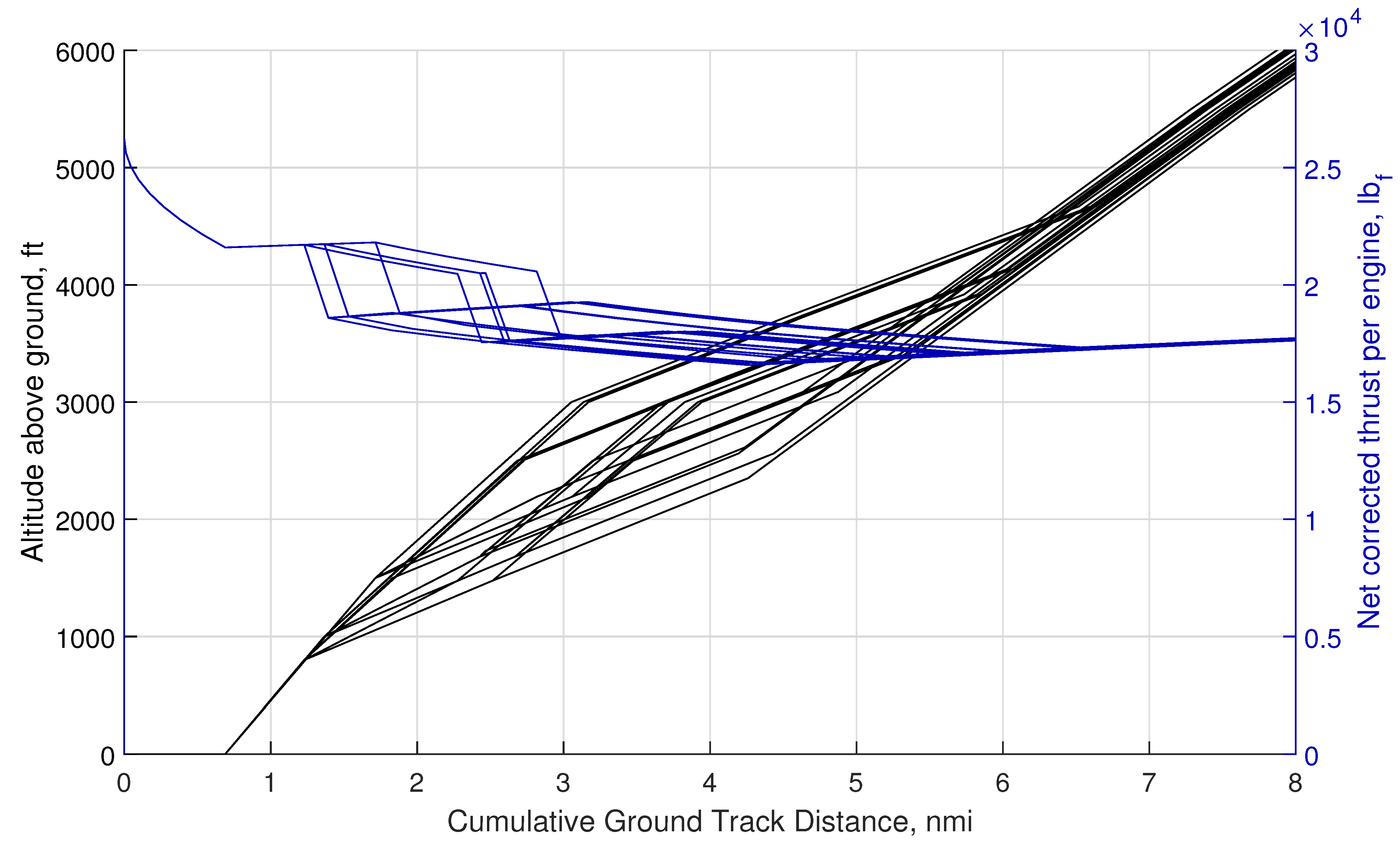
Variations in these different parameters can significantly alter the aircraft’s trajectory and thrust variation, both of which are primary contributors to departure noise. This variation is demonstrated in Figure 1. The NADP Library defined by Lim et al. [12] provides users with a set of 20 different NADP profiles which are suitable for modeling a large variety of operations that are typically observed in the real world [13,14]. Although higher fidelity data sources for aircraft movements are becoming more common as tracking and monitoring technology improves [15], obtaining noise quantification for each separate real-world observed trajectory remains elusive. In such cases, some data reduction technique such as clustering is often necessary in order to obtain environmental metrics [16].

2.2. Aviation Noise Quantification

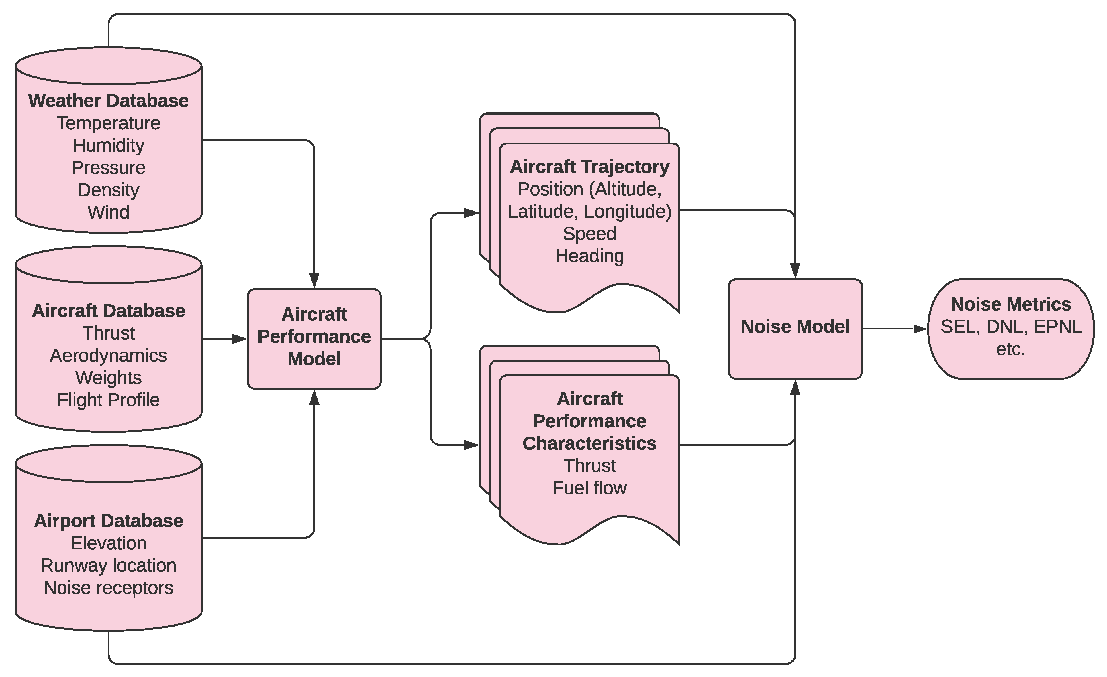
In this study, the data which is used as the input for reduced-order modeling is obtained from AEDT. AEDT is part of the FAA’s aviation environmental tool suite and replaces legacy modeling tools such as the integrated noise model and the emissions and dispersion modeling system [17]. A typical study in AEDT is built up by assigning aircraft operations to specific airport layouts. The tool then computes aircraft trajectories, performance characteristics along that trajectory, and then applies different noise metric models to calculate those metrics. A combination of physics-based and empirical models are used in this process. For example, the trajectory of the aircraft is computed using physics-based equations of motion, whereas the calculation of aircraft thrust levels are based on empirical equations (AEDT 3c Technical Manual: https://rosap.ntl.bts.gov/view/dot/49820/dot_49820_DS1.pdf?). The overall process is shown in Figure 2.

The core noise computations of AEDT are performed by certain modules that rely on different databases:

• Weather data—this consists of weather parameters such as temperature, humidity, pressure, density, and wind speed. These parameters affect not only the performance of the aircraft, but also the noise propagation through atmospheric absorption.
• Aircraft data—In order to compute the trajectory of the aircraft, several aircraft-specific parameters are required. The thrust and aerodynamic coefficients are required in order to compute the aircraft’s trajectory through fundamental performance equations. Additionally, the operational data relating to how a pilot might fly the aircraft is encoded through the profile, weight, and runway assignments.
• Airport data—the airport runways provide an anchor for the computed aircraft trajectory. Additionally, the airport also affects the weather through elevation, and historical weather data.
• Receptor sets—in order to compute community noise exposure, receptor sets have to be defined, which act as microphones where the desired noise metrics can be computed.

From Figure 2, it is evident that the noise metrics depend on the aircraft trajectory and performance characteristics, which, in turn, are dependent on the input databases. Due to these underlying dependencies, there are a large number of parameters that affect the computed noise. When trying to quantify noise metrics from real-world operations, this isn’t a problem, as it represents a few relatively fixed values of the parameters. However, in order to perform an optimization of noise metrics, it is necessary to explore a much larger “design space” of parameters, which is presently not possible due to the computational constraints.

2.3. Existing Methods on Rapid Noise Quantification

There have been several efforts to improve the computational efficiency of AEDT in the past few years. Bernado et al. developed a method to perform noise computations for generic fleets, using some simplifying assumptions, and pre-calculated noise results [18]. The primary assumption which facilitates this framework is straight-in and straight-out ground tracks, no environmental variations, and sea-level airports. The assumptions of non-curved ground tracks lead to a symmetric noise grid, which, along with the other assumptions, greatly reduces the amount of pre-calculated data that has to be stored. The stored results can then be combined using appropriate computations into the results for a fleet-level analysis. This methodology yielded benefits to both the set-up time and the computational time, however, the applicability of the method was severely curtailed due to the assumptions. The results were only accurate at a very limited number of scenarios that matched the assumed conditions.

In order to truly capture accurate results across a wider range of parameters, pre-computed grids are insufficient, and true surrogate modeling is required. Levine et al. tried to include weather parameters and aircraft takeoff weight effects on the noise grids [19]. This was done by creating a calibration model that would act on standard day sea-level noise grids and improve their accuracy. Some assumptions such as straight ground tracks were retained. Several different surrogate modeling techniques were investigated including Response Surface Methodology (RSM), Kriging interpolation techniques, and Artificial Neural Networks with a single layer, and with double layer. The Artificial Neural Network with 2 layers was found to be the most accurate among the tested methods. Although the computed $R^2$ values were quite high, the error at some validation test cases was quite high. Additionally, it was found that the error grew at higher decibel levels, which is undesirable from the context of evaluating noise mitigation efforts.

The Proper Orthogonal Decomposition (POD) method applied to AEDT has shown encouraging results for rapid noise predictions [20]. The researchers made use of POD for the orthonormal basis extraction, and ordinary Kriging for the basis coefficient prediction. The technique was demonstrated on two AEDT outputs—departure and approach noise, with five weather parameters used for the input variation. These parameters were—airport elevation, temperature, pressure, relative humidity, and headwind. The technique was demonstrated on a single aircraft type, and for operations performed on straight ground tracks. Additionally, no variation was introduced for the aircraft starting weight. The Sound Exposure Level (SEL) noise metric was considered at a grid superimposed along the half area at one side of the ground track. This area was modeled as a rectangular region of 32 × 16 nmi, and was discretized into grid points with a spacing of 0.08 nmi, yielding 80,601 total points.

Two sets of 256 samples were created using a Latin hypercube Design Of Experiments (DOE) method. One set was used for the model fitting, and the other was used for model verification. This required a total of 512 evaluations by AEDT. The researchers used a batch mode version of AEDT called the AEDT Tester, which is faster to use than the AEDT GUI software. The results were then rearranged into the input for the POD. The predicted results showed good agreement with the verification results, and significant time savings were reported. These results encourage the application of ROM for an expanded set of parameters, which will further improve applicability and enable the construction of a true parametric design space exploration environment.

A common feature in all these efforts is the assumption of a fixed flight profile, usually, the default STANDARD profile which is defined in AEDT. While this default option does change depending on the aircraft, it does not capture any variability in the aircraft operation itself, which eliminates a significant portion of the design space. In this study, the POD-based method was be applied to create rapid noise models based on variation in an aircraft’s operation, while keeping a fixed airport with a straight ground track and a fixed aircraft.

2.4. Reduced Order Modeling

Reduced-order models allow for the prediction of field variables based on high fidelity analysis data. The use of ROMs in aerospace applications has been primarily in advanced Computational Fluid Dynamics applications such as those involving unsteady aerodynamics, aero-elastic effects, hypersonic flow fields etc. [21,22,23,24,25]. These models have also been used for multi-disciplinary design, analysis, and optimization applications such as the design optimization of airfoils [26]. The primary advantage of ROMs is that their evaluation is much faster than the underlying full-order models, thereby greatly increasing computational efficiency in the many-query context.

ROMs are a type of surrogate model created by using a set of snapshots (output results) from the full order model at a DOE of input parameter combinations. Interpolations are then used on the reduced-order model to predict results at untried parameter combinations.

ROMs can be either projection-based or interpolation-based. Projection-based methods operate using the underlying governing equations and are also known as intrusive methods. These types of ROMs are advantageous because they retain the underlying physics of the problem, if the underlying equations are known. Interpolation-based methods, on the other hand, are “non-intrusive” and do not rely on knowledge of the underlying physics of the problem, and perform interpolation directly on the reduced space. Due to the greater applicability of interpolation-based ROMs, they are used in this work.

There are several methods that can be employed to create the reduced space based on the Full-Order Model (FOM) snapshots. Some examples of methods are POD, Isomap, Fourier Model Reduction etc. In this study, the POD method will be used as it has been used previously in various aerospace applications, and is readily implemented in common programming languages such as MATLAB, and Python. The POD method determines the optimal linear basis of a high-dimensional space. While POD-based methods have found immense success in practice, they find a linear transformation between the high- and low-dimensional representations. Linear dimensionality methods are known to struggle with predicting highly localized nonlinear features but perform accurately globally. We defer the use of nonlinear dimension reduction methods to future work.

2.5. Research Contributions

Traditional quantification and mitigation efforts in the field of aviation community noise exposure have been hampered by the inherent complexity of the problem. This is a result of traditional scalar surrogates and full-order models being unable to efficiently capture the underlying field nature of noise metrics. The techniques developed in this work provide a method to address such shortcomings by adapting and implementing reduced-order modeling techniques to this problem.

3. Methodology

The overall methodology with all steps created for this work is explained in this section.

3.1. Experimental Case Setup

In order to correctly capture the underlying trends in a surrogate model, a large number of FOM results are needed. In this study, the objective is to test the ability of the ROM to capture the effects of parameters relating to the NADP profiles as defined in the NADP Library. The NADP Library consists of 20 profiles, of which 19 are modeled in this study. One profile, labeled as NADP1-5 was discarded as it required the implementation of a different type of thrust cutback, which is beyond the scope of this work. The remaining set of 19 profiles is divided into two categories—NADP1 and NADP2. NADP1 profiles delay acceleration in the initial phases in favor of higher climb rates. Thus, the aircraft can reach higher altitudes quicker, and thus alleviate the noise in the immediate vicinity of the airport. NADP2 profiles are suitable when the desired location of noise abatement is further downrange of the airport. In this type of NADP, the aircraft accelerates sooner, enabling it to retract flaps and achieve a clean configuration. Thus, the noise contribution from the airframe is reduced.

While the NADP Library consists purely of profile definitions, they can be modified to represent different aircraft take-off weights and thrust settings. Aircraft will often take-off with less than maximum thrust when it is safe to do so, this reduces the wear on the engines and helps airlines in reducing maintenance costs. AEDT allows for the definition of reduced thrust takeoffs. In this work, two different thrust sets are used—maximum and reduced. The maximum set makes use of maximum takeoff thrust and maximum climb thrust. The reduced set, denoted as “RT” uses 15% and 10% thrust reductions for takeoff and climb respectively.

Within AEDT, a profile may be flown at different stage lengths—an integer number denoting the distance flown by the aircraft. For example, a stage length of 4 indicates a great circle distance of 1500–2500 nmi. Each of these stage lengths then represents a takeoff weight for the aircraft, depending on the fuel load and an assumed load factor. AEDT provides two different weight options for each stage length—a legacy option, and an alternate option, denoted as “AW”. The alternate option weight is higher than the legacy option, primarily due to a higher load factor assumption.

With the thrust and weight options applied, four sets of NADP profiles are generated as shown in

Table 1. Profile set definitions.

Profile Set Label	Weight Set	Thrust Set	Stage Length
Normal	Legacy	Maximum	Minimum Median Maximum
AW	Alternate	Maximum
RT	Legacy	Reduced
AWRT	Alternate	Reduced

. Each of these sets are created and flown at three different stage lengths, denoting the smallest, median and longest distances that can be flown by the aircraft. In this situation the aircraft is the Boeing 737–800, which is one of the most common aircraft types in use globally.

With four sets of 19 profiles flown at three stage lengths, there are a large amount of variability in the trajectories and environmental impact of these operations. Unfortunately, the parameterization of the NADP Library included some non-continuous variables which are more complicated to deal with when creating surrogate models. Therefore the complete set of NADP profiles had to be reduced to the largest possible subset with a common structure for parameterization. Any surrogate mode requires a common parameterization structure to describe all training and validation cases. In the absence of such a structure, separate models need to be created for each subset of cases for which such a common representation can be obtained. The process involved conversion from descriptive variables to continuous variables and is summarized in

Table 2. Adaptation of the original NADP Library to create a suitable subset for Reduced-Order Modeling (ROM) modeling.

Profile #	Original Definition				Adapted Definitions
	Profile	Thrust Cutback	Initial Accel	Final Accel	Thrust Cutback Type	Converted Thrust Cutback	Final Accel Type	Included in Modeling?
1	NADP1_1	800 ft	1500 ft	3000 ft	Altitude	800 ft	Altitude	N
2	NADP1_2	800 ft	2500 ft	CONT	Altitude	800 ft	Speed	Y
3	NADP1_3	800 ft	3000 ft	CONT	Altitude	800 ft	Speed	Y
4	NADP1_4	1000 ft	2500 ft	CONT	Altitude	1000 ft	Speed	Y
5	NADP1_6	1000 ft	3000 ft	CONT	Altitude	1000 ft	Speed	Y
6	NADP1_7	1500 ft	3000 ft	CONT	Altitude	1500 ft	Speed	Y
7	NADP2_1	1500 ft	1000 ft	1500 ft	Altitude	1500 ft	Altitude	N
8	NADP2_2	AFTER	800 ft	3000 ft	Speed	N.A.	Altitude	N
9	NADP2_3	AFTER	1000 ft	3000 ft	Speed	N.A.	Altitude	N
10	NADP2_4	AFTER	1000 ft	2500 ft	Speed	N.A.	Altitude	N
11	NADP2_5	AFTER	1000 ft	CONT	Speed	N.A.	Speed	N
12	NADP2_6	AFTER	1500 ft	CONT	Speed	N.A.	Speed	N
13	NADP2_7	BEFORE	800 ft	3000 ft	Altitude	800 ft	Altitude	N
14	NADP2_8	BEFORE	800 ft	CONT	Altitude	800 ft	Speed	Y
15	NADP2_9	BEFORE	1000 ft	2500 ft	Altitude	1000 ft	Altitude	N
16	NADP2_10	BEFORE	1000 ft	CONT	Altitude	1000 ft	Speed	Y
17	NADP2_11	BEFORE	1000 ft	3000 ft	Altitude	1000 ft	Altitude	N
18	NADP2_12	BEFORE	1500 ft	CONT	Altitude	1500 ft	Speed	Y
19	NADP2_13	BEFORE	1500 ft	3000 ft	Altitude	1500 ft	Altitude	N

. Note that NADP1_5 from the original NADP Library is excluded as it requires the implementation of deep thrust cutback, which is beyond the scope of this work.

NADP profiles are characterized by three parameters called—CUTBACK, INITIAL ACCEL, and FINAL ACCEL. CUTBACK describes how thrust cutback is performed. A numeric value indicates an altitude based cutback, where the transition is made once the aircraft reaches a certain altitude. Cutback can also be based on the flap retraction schedule. AFTER is used to describe the situation in which the thrust cutback is performed after the aircraft reaches a clean configuration. BEFORE describes a cutback performed concurrently with the initiation of the flap retraction schedule. The initiation of the flap retraction schedule is always described by an altitude, and thus the descriptive BEFORE can be changed into numeric altitude values. The second mixed-value variable is FINAL ACCEL, which similarly can be both altitude-based or speed-based. In this situation, all profiles with an altitude definition for this variable were discarded.

With this reduction of the NADP Library, the subset contains 8 profile definitions. Variations from the weight and thrust options are retained, giving a total of $8\times 4\times 3=96$ total cases.

All cases were simulated in AEDT for the Boeing 737800 at Atlanta airport with noise being recorded at a receptor grid of $231\times$ 61 = 14,091 points spaced $0.1$ nmi in both the North-South, and East-West directions. The spacing between grid points was chosen based on sensitivity analysis for different spatial discretizations as explained in Section 4.6. The airport averaged weather setting was selected in AEDT, which accounts for variations of ambient temperature, pressure, and density with altitude. The effect of wind on sound propagation is not considered in AEDT and subsequently by the results of our model.

3.2. Proper Orthogonal Decomposition with Interpolation in Latent Space

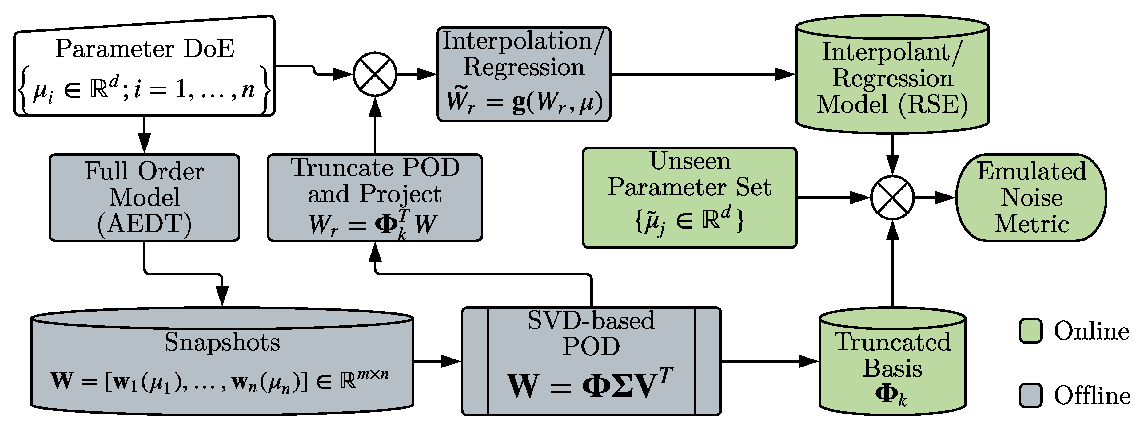
The basic procedure utilizes the POD method on a set of snapshots (full-order solutions at different parameter locations) to compress and obtain a low-dimensional basis set. The training data is then projected onto the reduced space to obtain coordinates of the high-dimensional system in the latent space. The encoded form of the parametric variation is obtained by creating a map between the parameter space and coordinates in the latent space. Interpolation and/or regression techniques from machine-learning are usually utilized to learn this map. Figure 3 shows the general process and the offline-online decomposition for the method.

In this approach, the offline phase consists of evaluating the full order model (i.e., AEDT, in this work) at a set of predetermined points in the input parameter space as specified by a DOE. Note that the success of any surrogate modeling approach depends on thorough coverage of the input design space. This work utilizes a full-factorial DOE as described previously to generate 96 input points that cover the design space in a structured fashion. Once snapshot data is collected, the POD is employed to reduce the dimensionality and find a lower-dimensional basis set (${\mathsf{\Phi }}_k$). The full order solutions are then projected onto the subspace spanned by the range of ${\mathsf{\Phi }}_k$. Each latent space coordinate is treated as a scalar that is a function of the parameters. The DOE in conjunction with the reduced coordinates are used to train scalar surrogate models to serve as maps between parameters and lower dimensional coordinates. At a new (unseen) point in the parameter space, a linear combination of the truncated basis sets and the predicted latent space coordinates is used to emulate the field.

Some of the well-known earliest uses of such approaches were by Ly et al. [27] and Bui-Tanh et al. [28]. In both these papers, authors use cubic splines to create interpolants for the coefficients as functions of the parameters and demonstrate accurate field emulation at points not used in the training process. Authors [29,30,31,32,33,34] have relied on radial basis functions for the reduced space coordinate surrogates. Mainini et al. [35] used the POD method along with response surfaces and self-organizing maps to enable real-time structural capability assessment. Recently, researchers [36,37] have experimented with the usage of artificial neural networks for the reduced coordinates. In related work by Xiao et al. [38], sparse grids and Taylor series expansions were used to predict coefficients with time as the only parameter. Authors [33,39,40,41] have also used Gaussian processes for capturing parametric dependence of the latent space coordinates.

The following notations and mathematical definitions are used throughout the paper:

• $\mathit{w}(\mathit{x},\mathbf{\mu })\in {\mathbb{R}}^m$ is the finite-dimensional representation of the noise metric solutions from a full-order model.
• $\mathit{x}$ is the location where the noise metrics are evaluated.
• $\mathit{\mu }\in {\mathbb{R}}^d$ denotes the parameters which influence the results of the FOM as a vector. For example, Profile 2 in Table 2 when flown at reduced thrust and 145,500 lbs takeoff weight is represented as [800, 2500, 145,500, 0.85]. Note that 800 represents the altitude of thrust cutback, 2500 represents the altitude where acceleration is initiated, and 0.85 represents a 15% reduction applied to the maximum takeoff thrust.
• $m\gg 1$ denotes the high-dimensional field output, which in this context is in the $\mathcal{O}\left({10}^5\right)$.
• $\mathit{W}=[\mathit{w}\left({\mathit{\mu }}_1\right),\mathit{w}\left({\mathit{\mu }}_2\right),\cdots ,\mathit{w}\left({\mathit{\mu }}_n\right)]\in {\mathbb{R}}^{m\times n}$ is the snapshot matrix. In ROM literature, the snapshot matrix is a collection of solutions at various parameter values $\{{\mathit{\mu }}_i,i=1,2,\cdots ,n\}$.

Wherever it is obvious, the dependence of $\mathit{w}$ on $\mathit{\mu }$ may not be explicitly mentioned for the sake the brevity. A subscript index into the set of parameter points is used instead.

Step 1: Computation of the POD Modes via Singular Value Decomposition (SVD)

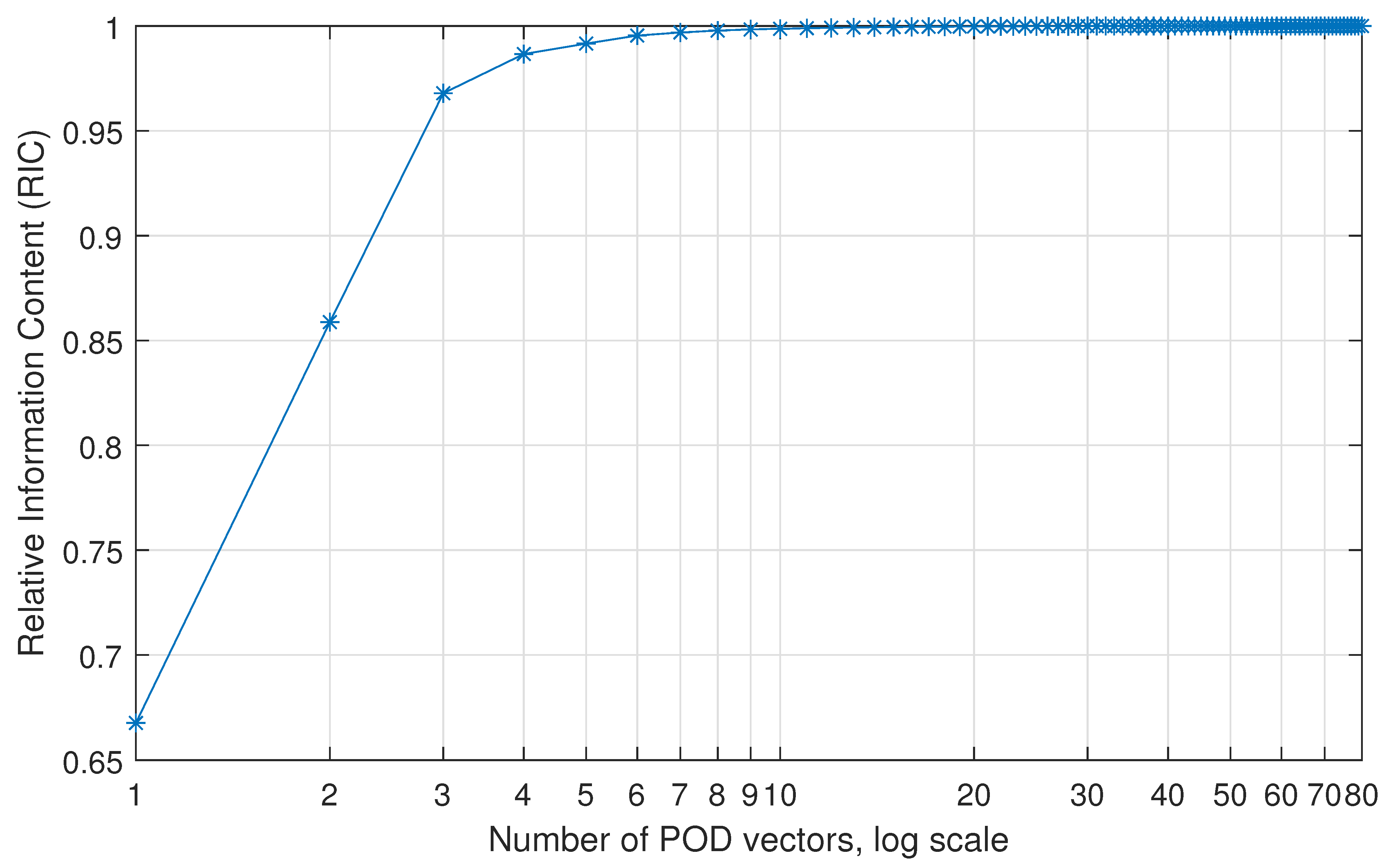
Following the creation of a DOE and evaluation of the full order model, the snapshot matrix $\mathit{W}$ is compressed using the Singular Value Decomposition method to compute the first k dominant POD modes. The choice of k depends on the cutoff value selected for the Relative Information Content (RIC). The RIC is a metric used to rank the columns of ${\mathsf{\Phi }}_k$ according to their importance and is calculated using the singular values ${\sigma }_i$ in the matrix ${\Sigma }_k$ arranged in descending order.

$$\mathit{W}\approx {\mathsf{\Phi }}_k{\Sigma }_k{\mathit{V}}_k^T$$

(1)

$${\sigma }_i=\Sigma [i,i]$$

(2)

$$RI{C}_j=\frac{{\sum }_{i=1}^j{\sigma }_i^2}{{\sum }_{i=1}^m{\sigma }_i^2}$$

(3)

where $\mathit{W}\in {\mathbb{R}}^{m\times n}$, ${\mathsf{\Phi }}_k\in {\mathbb{R}}^{m\times k}$, ${\Sigma }_k\in {\mathbb{R}}^{k\times k}$, and ${\mathit{V}}_k\in {\mathbb{R}}^{n\times k}$ such that $k\ll m$. The POD decomposition minimizes reconstruction error in the $L_2$ norm.

Step 2: Expressing Solution in the POD basis

The POD modes obtained using SVD are a basis set that can be used to express the FOM solution as:

$$\overline{\mathit{w}}=\frac{{\sum }_{i=1}^n{\mathit{w}}_i}{n}$$

(4)

$${\mathit{w}}^{\prime }=\mathit{w}\left(\mathit{\mu }\right)-\overline{\mathit{w}}\approx \sum _{j=1}^k{a}_j\left(\mathit{\mu }\right){\mathit{\varphi }}_j$$

(5)

$$a_j\left(\mathit{\mu }\right)=\langle \mathit{w}\left(\mathit{\mu }\right)-\overline{\mathit{w}},{\mathbf{\varphi }}_j\rangle =\langle {\mathit{w}}^{\prime }\left(\mathbf{\mu }\right),{\mathbf{\varphi }}_j\rangle$$

(6)

Once the POD-basis is computed, projected coordinates or coordinates in the latent space are obtained using Equation (6) for all the snapshots in $\mathit{W}$ to obtain ${\mathit{W}}_r$.

Step 3: Train Surrogates in the Latent Space via supervised learning techniques

The last step of the training process involves the creation of surrogate models treating each of the k expansion coefficients as scalar functions of the parameters. As mentioned before, any technique from machine learning theory can be employed to create these scalar functions. This study employs the response surface methodology to estimate the projection coordinates which assumes a second-degree polynomial as the functional form.

$$a_j\left(\mathbf{\mu }\right)={\mathit{g}}_j(\mathbf{\mu };{\mathit{W}}_r)$$

(7)

where $\mathit{g}:{\mathbb{R}}^d\to {\mathbb{R}}^k$ is the learned map between the parameters and the input space.

Note that more advanced techniques such as Gaussian Processes, Deep Gaussian Processes [42], Artificial Neural Networks etc. can be employed but typically require a much larger training dataset in order to provide good predictions. For this problem, these methods tended to displayed signs of overfitting on the training data and resulted in large errors in the validation data predictions. The RSM utilized here strikes a good balance between the amount of data required and the accuracy of the prediction.

Step 4: Emulate Field at Unseen Parameter Point

Once the ROM is trained in steps 1-3, the following expression approximates the field at an unseen parameter point $\tilde{\mathbf{\mu }}$ rapidly. Note that this prediction is much faster than a FOM evaluation due to the fact that use of the ROM simplifies the problem to the prediction of a few scalars, rather than a high dimensional dataset.

$${\mathit{w}}_{pred}\left(\tilde{\mathbf{\mu }}\right)=\overline{\mathit{w}}\left(\mathbf{\mu }\right)+\tilde{\mathsf{\Phi }}\mathit{g}(\tilde{\mathbf{\mu }};{\mathit{W}}_{\mathit{r}})$$

(8)

where $\tilde{\mathsf{\Phi }}=\left[\widetilde{{\mathbf{\varphi }}_1},\widetilde{{\mathbf{\varphi }}_2},\cdots ,\widetilde{{\mathbf{\varphi }}_k}\right]\in {\mathbb{R}}^{m\times k}$ denotes the POD basis.

3.3. Validation of Methodology

The results obtained in Step 4 are validated against the FOM results for the allocated 16 validation cases. Two validation analyses are performed—first, the prediction capability of the RSM surrogate model is tested by projecting the validation cases onto the reduced space and comparing the obtained coefficients of projections against their predicted values.

The second validation is a direct comparison of the noise grid obtained by the methodology against the noise grid obtained from the FOM. This comparison is performed quantitatively and also visually with contour plots.

4. Implementation and Results

This section describes the results obtained at each major step of the method, and the associated errors. There are two main sources of error introduced in the method. The first main source of error arises from the projection of the full order model solutions onto the reduced space representation. The other main source of error is the surrogate model or interpolation scheme which is developed to make predictions.

The results from AEDT are compiled as vectors of length 14,091 $\times 1$. There are 96 such vectors, which are randomly divided into 2 groups—80 training sets and 16 validation cases. These two datasets can be represented as two matrices—${\mathit{W}}_{train}$ and ${\mathit{W}}_{valid}$, with $14,091$ rows each, and 80 and 16 columns respectively.

4.1. Results for POD Basis Selection

The RIC vector helps inform the choice of the number of POD vectors which are used as the basis to create the lower order representation. More POD vectors retain more information, but have diminishing returns, as shown in Figure 4. In this study, an RIC of 0.999 is desired, for which 11 POD vectors $\left\{{\mathbf{\varphi }}_{\mathbf{1}},{\mathbf{\varphi }}_{\mathbf{2}},\cdots ,{\mathbf{\varphi }}_{\mathbf{11}}\right\}$ are selected as the basis for the lower order representation.

4.2. Results for Lower Order Projection

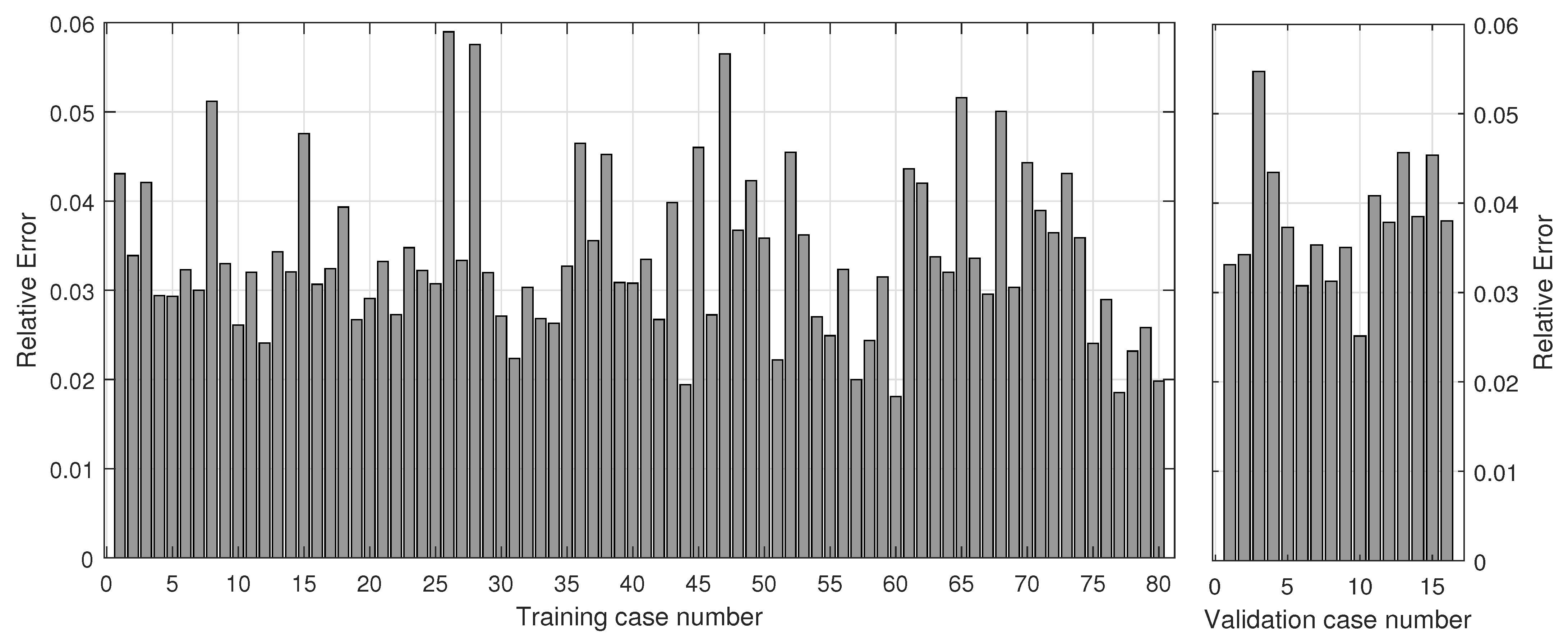
The error associated with the lower order projections arise from the fact that input vectors to the POD process do not completely lie within the space spanned by the POD vectors. This error is directly related to the number of POD vectors chosen as the basis of the reduced space. Choosing more POD vectors for the basis will result in a smaller projection error, at the expense of a larger number of surrogate models being required. Any orthogonal components to this reduced space are manifested by a projection error, which can be obtained by subtracting the projected vector from the original vector.

$${\mathit{e}}_{\mathit{proj}}=\sum _{j=1}^k{a}_j\left(\mathbf{\mu }\right){\mathbf{\varphi }}_j-{\mathit{w}}^{\prime }$$

(9)

$$=\sum _{j=1}^k\langle {\mathit{w}}^{\prime }\left(\mathbf{\mu }\right),{\mathbf{\varphi }}_j\rangle {\mathbf{\varphi }}_j-{\mathit{w}}^{\prime }$$

(10)

$${\mathit{e}}_{\mathit{proj},\mathit{rel}}=\left[\frac{\left|\right|{\mathit{e}}_{\mathit{proj},\mathit{i}}\left|\right|}{\left|\right|{{\mathit{w}}^{\prime }}_i\left|\right|}\right]$$

(11)

The magnitude of this relative error is calculated using the standard Euclidean vector norm, and is shown in Figure 5. It is observed that the error due to this projection is in the range of 2% to 6%. Note that this error quantification is with respect to the results from which the mean noise vector has been subtracted. Therefore 6% projection error implies an inaccuracy of 6% in the variation of the noise vector from the mean noise vector for that case, and not a 6% inaccuracy in the noise dB values themselves.

In addition to the relative error, the absolute error is also analyzed and presented in

Table 3. Summary statistics of projection error components.

Dataset	Min dB SEL	Max dB SEL	Mean dB SEL	Median dB SEL	Range dB SEL	Standard Deviation dB SEL
Training	$-1.2505$	$1.3959$	$-8.5975\times {10}^{-18}$	$6.0876\times {10}^{-4}$	$2.6464$	$0.0459$
Validation	$-1.0402$	$1.1643$	$6.4492\times {10}^{-4}$	$-6.4776\times {10}^{-4}$	$2.2044$	$0.0540$

. This table provides summary statistics for the error at each component in ${\mathit{e}}_{\mathit{proj}}$.

4.3. Surrogate Model Predictions and Error

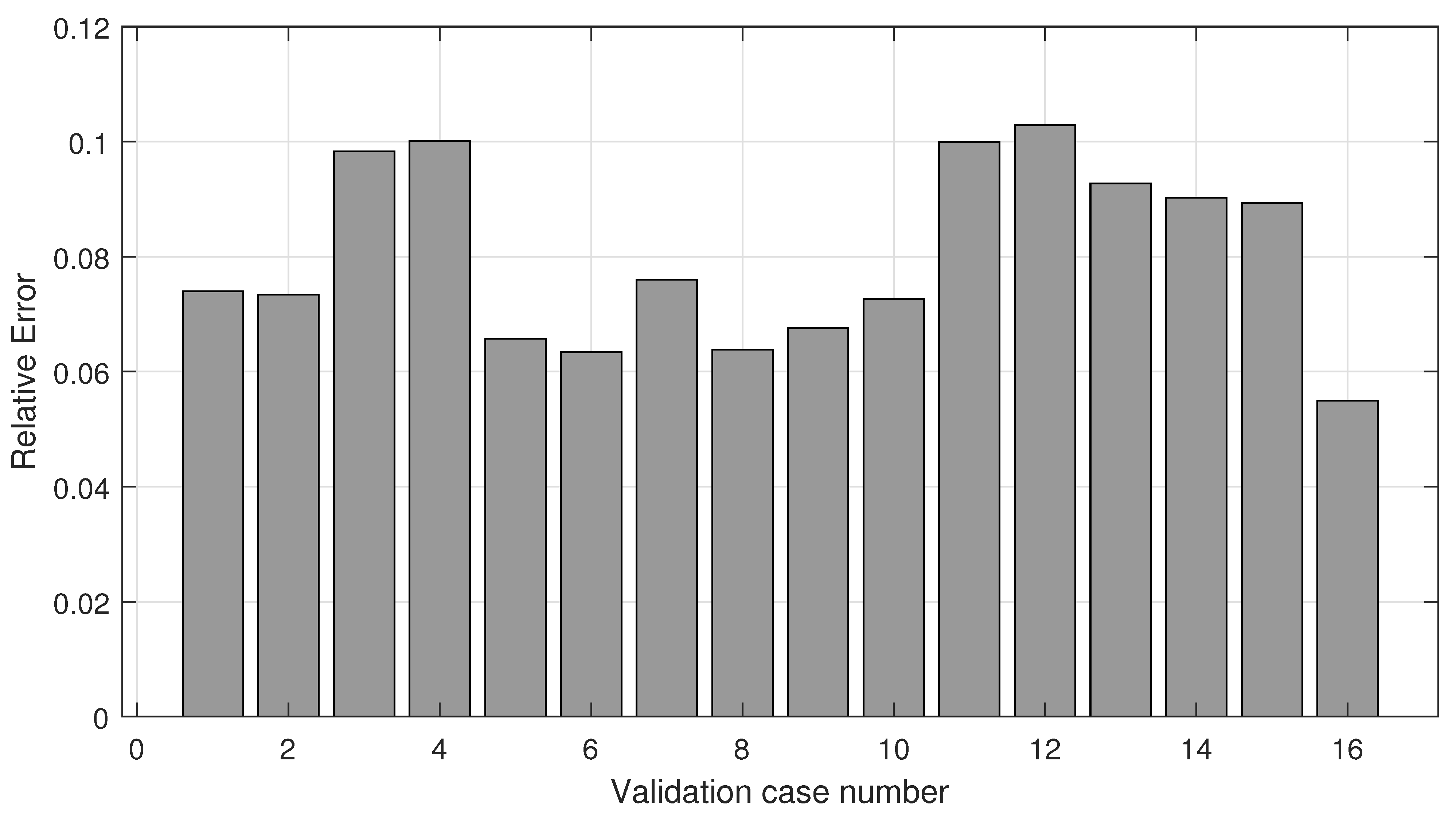
Using the created RSM models for each of 11 components ${\mathit{a}}_j\left(\mathbf{\mu }\right)$, the projected dataset of the 16 validation cases was predicted. This was then compared with the true projections of the validation datasets, in order to compute the error attributable to the surrogate modeling process.

$${\mathit{w}}_{pred}^{\prime }\left(\tilde{\mathbf{\mu }}\right)=\mathsf{\Phi }\mathit{g}(\tilde{\mathbf{\mu }};{\mathit{W}}_{\mathit{r}})$$

(12)

$${\mathit{w}}_{true}^{\prime }\left(\tilde{\mathbf{\mu }}\right)=\sum _{j=1}^k\langle {\mathit{w}}^{\prime }\left(\tilde{\mathbf{\mu }}\right),{\mathbf{\varphi }}_j\rangle {\mathbf{\varphi }}_j$$

(13)

$${\mathit{e}}_{pred}={\mathit{w}}_{pred}^{\prime }\left(\tilde{\mathbf{\mu }}\right)-{{\mathit{w}}^{\prime }}_{true}\left(\tilde{\mathbf{\mu }}\right)$$

(14)

$${\mathit{e}}_{pred,rel}=\left[\frac{\left|\right|{\mathit{e}}_{pred,i}\left|\right|}{\left|\right|{{\mathit{w}}^{\prime }}_{true,i}\left|\right|}\right]$$

(15)

Similar to the projection error, the magnitude of this error is computed using the standard vector norm and is shown in Figure 6. It is observed that the relative error varies from about 6% to 10%. It should be noted that, as with the projection error, this error is calculated on the mean subtracted noise vectors. Therefore, this error represents the loss of accuracy due to the surrogate model used to predict the coefficients ${\alpha }_i$.

In addition to the relative error, the absolute error is also analyzed and presented in

Table 4. Summary statistics of prediction error components.

Dataset	Min dB SEL	B dB SEL	Mean dB SEL	Median dB SEL	Range dB SEL	Standard Deviation dB SEL
Validation	$-1.7118$	$1.9766$	$0.0010$	$0.0012$	$3.6884$	$0.1152$

. This table provides summary statistics for each component of the error matrix ${\mathit{e}}_{pred}$. It is observed that these errors are slightly higher compared to those observed in the projection step of the process. The error associated with prediction can be reduced by including a higher number of training cases which can be used to build a more accurate surrogate model. However, conscious efforts must be made to prevent the surrogate model from an overfit to the input parameters.

4.4. Combined Errors

In the previous subsections, the individual errors for the projection and prediction step of the process were isolated and analyzed. In order to assess the efficacy of the process, the total error in terms of the final predicted noise grids v/s the original noise grids must be considered.

$${\mathit{e}}_{total,rel}=\left[\frac{\left|\right|\overline{\mathit{w}}\left(\mathbf{\mu }\right)+\tilde{\mathsf{\Phi }}\mathit{g}(\tilde{\mathbf{\mu }};{\mathit{W}}_{\mathit{r}})-\mathit{w}(\mathit{x},\tilde{\mathbf{\mu }})\left|\right|}{\left|\right|\mathit{w}(\mathit{x},\tilde{\mathbf{\mu }})\left|\right|}\right]$$

(16)

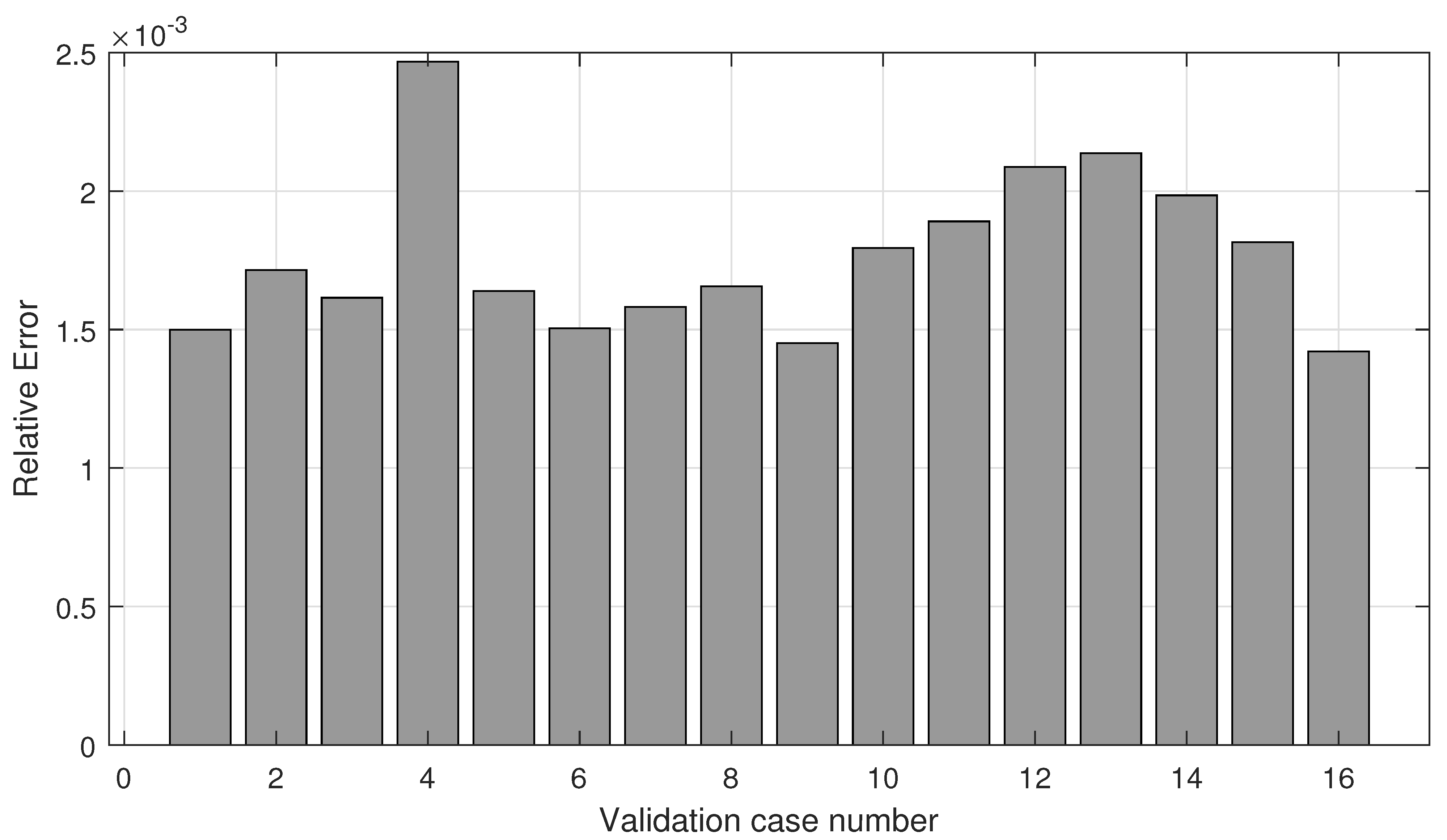
Figure 7 shows the total relative error for each of the 16 validation cases. Note that this error is a direct measure of the difference in the predicted noise grids, and the respective FOM results. It is observed that the total error varies from 0.14% to 0.25% which implies that most of the noise grid was replicated accurately by the process.

The absolute total errors are tabulated as summary statistics in

Table 5. Summary statistics of total error components.

Dataset	Min dB SEL	Max dB SEL	Mean dB SEL	Median dB SEL	Range dB SEL	Standard Deviation dB SEL
Validation	$-1.7089$	$1.6349$	$0.0017$	$0.0028$	$3.3438$	$0.1272$

. The maximum error at any grid point across the 16 validation cases was an underestimation by 1.71 dB, and an overestimation by 1.63 dB. While these values may seem quite large, the mean, median, and standard deviation errors are all quite small, indicating that the min and max error cases are outliers, and that much of the $231\times 61$ noise grid has been accurately reconstructed.

4.5. Reconstructed Noise Grids

The objective of this ROM methodology is to enable the prediction of noise grids at airports for a variety of different conditions. In this study, the variation between test cases arises from the usage of different operational profiles by the same aircraft. Therefore, the best evaluation of the process is a direct comparison of the noise grid predictions with the original FOM data.

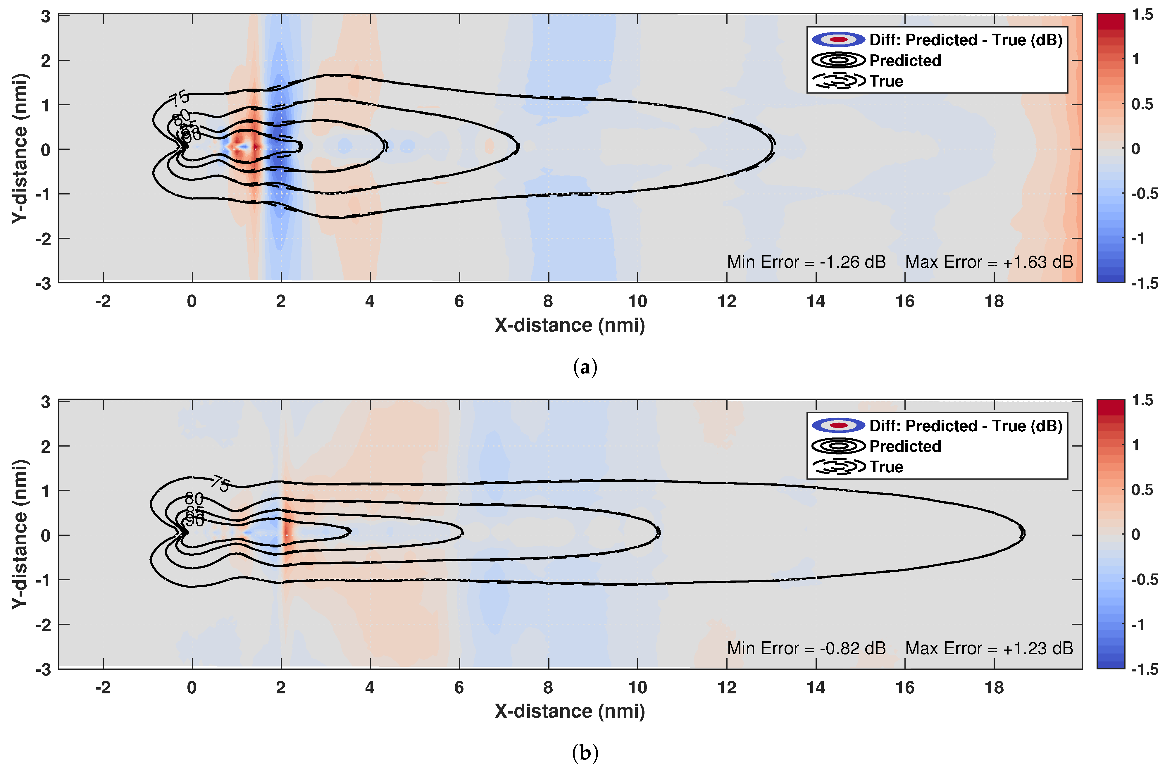
Here, two different comparisons representing two of the 16 validation cases are shown, corresponding to the cases with the minimum and maximum error as observed in Figure 7. Comparisons are made directly on the noise grid difference between the true and the predicted values with a colormap background, overlaid with contours, which are a typical visualization used to depict community noise exposure. These comparisons are shown in Figure 8.

It is observed from these figures that the methodology successfully replicates the original noise grid for a large part of the noise grid. Most of the differences are also small in magnitude, with the largest errors being observed in isolated pockets close to the 90 dB contour. The accuracy of the method is also confirmed by the contour plots which are recreated accurately. In Figure 8a, it is observed that the predicted 90 dB contour diverges from the true 90 dB contour for a small region. The error in this region can most likely be attributed to the thrust cutback step of the aircraft’s departure operation. The thrust cutback represents a change in thrust from takeoff setting to climb setting, which can act as a “jump” discontinuity, which introduces a non-linearity in the noise grid. The POD method investigated in this research tries to represent the noise grid with linear approximations, and thus gives a slightly higher error in this region. However, even with a linear approximation, the error is limited to $\pm 1.5$ dB SEL.

The four sets of contours in each plot are also compared quantitatively in

Table 6. Summary statistics of total error components.

Validation Case	Contour Level	FOM Results			Recreated Results			Differences
		Length (nmi)	Width (nmi)	Area (nmi2)	Length (nmi)	Width(nmi)	Area (nmi2)	Length	Width	Area
Highest Total Error	75 dB	13.98	3.18	31.25	13.91	3.22	31.09	−0.50%	1.26%	0.51%
	80 dB	7.89	2.09	11.88	7.86	2.13	11.88	−0.38%	1.91%	0%
	85 dB	4.73	1.14	4.37	4.65	1.17	4.33	−1.69%	2.63%	−0.92%
	90 dB	2.70	0.71	1.35	2.66	0.75	1.27	−1.48%	5.63%	5.93%
Lowest Total Error	75 dB	19.56	2.47	39.46	19.62	2.46	39.40	0.31%	−0.40%	−0.15%
	80 dB	11.09	1.63	13.35	11.04	1.63	13.29	−0.45%	0%	−0.45%
	85 dB	6.46	1.03	4.59	6.44	1.01	4.62	−0.31%	−1.94%	0.65%
	90 dB	3.86	0.68	1.66	3.79	0.68	1.66	−1.81%	0%	0%

. It is seen that most contour dimensions are recreated accurately. The largest relative error is observed for the 90 dB SEL contour width. This can be traced back to the non-linear effects of thrust cutback, and the subsequent linear representation using the POD method.

4.6. Discussion on Grid Discretization

The results shown in the previous subsections are based on noise results which are computed on a grid of noise sensors defined with a spacing of 0.10 nmi. A sensitivity to grid spacing was performed to determine the appropriate level of discretization. A total of three grid spacing options were considered, and it was found that the grid spacing among these settings does not have a significant impact on the POD computation. The results of this sensitivity analysis are shown in

Table 7. Sensitivity of POD to noise grid discretization.

Grid #	Spacing (nmi)	Grid Dimensions		RIC for POD Mode Index (Percentages, %)
		Number of Grid Points	Length (nmi) × Width (nmi)	1	3	5	7	9	11
1	0.08	289 × 76 = 21,964	23.04 × 6	66.516	96.733	99.147	99.683	99.833	99.909
2	0.10	231 × 61 = 14,091	23.00 × 6	66.667	96.726	99.146	99.684	99.836	99.911
3	0.12	193 × 51 = 9843	23.04 × 6	66.825	96.750	99.157	99.689	99.838	99.912

.

From Table 7, it is seen that the RIC value does not change appreciably across different grid discretizations. Choosing a fine grid (0.08 nmi spacing) provides no additional benefit, while simultaneously increasing the number of grid points required to cover the same geographic area. This increases the amount of data to be computed, stored, and processed which leads to slower overall processing times. Therefore, the grid should be discretized at a level that produces sufficiently smooth noise contours. To this effect, a grid spacing of 0.10 nmi was chosen for the results shown here.

4.7. Discussion of Results

The results obtained by the methodology successfully replicate, to a large extent, the results from the original full-order model (AEDT). The comparison between the results from AEDT and the methodology was made at 16 validation cases representing a variety of different operational procedures flown by aircraft. Even in the prediction with the highest error, much of the noise grid is successfully replicated. Regions of larger error are noticed at the 90 dB contour line, which might warrant further investigation.

5. Conclusions

This study demonstrated the use of ROM in the context of aviation community noise quantification. Specifically, the POD method was used in conjunction with RSM to create a framework for the prediction of noise grids around an airport for a single aircraft flying under different operational procedures. A total of 80 cases were used to train the model, and 16 cases were used for validation. The framework was able to recreate the noise grids with sufficient accuracy and encourages the exploration of a more comprehensive study in this area.

The primary advantage of using a ROM methodology in the context of aviation noise predictions is that it enables the development of rapid noise quantification tools that can be used to perform parametric analyses and optimizations, which are not possible with full order models alone. The other advantage offered by ROMs is that they are able to provide field predictions rather than scalar, point predictions like traditional surrogate models. This method is beneficial for a wide variety of optimization scenarios such as those involving the design of an aircraft trajectory, or for noise insulation investment decisions. With these advantages, future work can expand upon this methodology to address curved ground tracks, multiple aircraft types, generic airport definitions etc.

References

- Federal Aviation Administration. Federal Aviation Administration Aerospace Forecasts Fiscal Years 2019–2039; U.S. Dept. of Transportation, Federal Aviation Administration, Office of Aviation Policy and Plans: Washington, DC, USA, 2019. Available online: https://www.faa.gov/data_research/aviation/aerospace_forecasts/media/FY2019-39_FAA_Aerospace_Forecast.pdf (accessed on 20 January 2021).
- International Civil Aviation Organization’s CO2 Standard for New Aircraft. 2016. Available online: https://theicct.org/sites/default/files/publications/ICCT-ICAO_policy-update_feb2016.pdf (accessed on 20 January 2021).
- International Civil Aviation Organization. Annex 16—Environmental Protection—Volume I—Aircraft Noise. 2017. Available online: https://store.icao.int/en/annex-16-environmental-protection-volume-i-aircraft-noise (accessed on 20 January 2021).
- Ganic, E.; Dobrota, M.; Babic, O. Noise abatement measures at airports: Contributing factors and mutual dependence. Appl. Acoust. 2016, 112, 32–40. [Google Scholar] [CrossRef]
- Ganić, E.; Babić, O.; Čangalović, M.; Stanojević, M. Air traffic assignment to reduce population noise exposure using activity-based approach. Transp. Res. Part D Transp. Environ. 2018, 63, 58–71. [Google Scholar] [CrossRef]
- Basner, M.; Clark, C.; Hansell, A.; Hileman, J.I.; Janssen, S.; Shepherd, K.; Sparrow, V. Aviation Noise Impacts: State of the Science. Noise Health 2017, 19, 41–50. [Google Scholar] [CrossRef] [PubMed]
- Correia, A.W.; Peters, J.L.; Levy, J.I.; Melly, S.; Dominici, F. Residential exposure to aircraft noise and hospital admissions for cardiovascular diseases: Multi-airport retrospective study. BMJ 2013, 347. [Google Scholar] [CrossRef] [Green Version]
- Klatte, M.; Bergström, K.; Lachmann, T. Does noise affect learning? A short review on noise effects on cognitive performance in children. Front. Psychol. 2013, 4, 578. [Google Scholar] [CrossRef] [Green Version]
- Jiao, B.; Zafari, Z.; Will, B.; Ruggeri, K.; Li, S.; Muennig, P. The Cost-Effectiveness of Lowering Permissible Noise Levels Around U.S. Airports. Int. J. Environ. Res. Public Health 2017, 14, 1497. [Google Scholar] [CrossRef] [PubMed] [Green Version]
- International Civil Aviation Organization Doc 8168 OPS/611 Procedures for Air Navigation Services, Aircraft Operations: Volume I Flight Procedures. 2006. Available online: https://store.icao.int/en/procedures-for-air-navigation-services-pans-aircraft-operations-volume-i-flight-procedures-doc-8168 (accessed on 20 January 2021).
- Federal Aviation Administration Advisory Circular 91-53A—Noise Abatement Departure Profiles. 1983. Available online: https://www.faa.gov/documentLibrary/media/Advisory_Circular/ac91-53.pdf (accessed on 20 January 2021).
- Lim, D.; Behere, A.; Jin, Y.C.; Li, Y.; Kirby, M.; Gao, Z.; Mavris, D.N. Improved Noise Abatement Departure Procedure Modeling for Aviation Environmental Impact Assessment; AIAA Scitech 2020 Forum: Orlando, FL, USA, 2020. [Google Scholar] [CrossRef]
- Behere, A.; Lim, D.; Li, Y.; Jin, Y.C.; Gao, Z.; Kirby, M.; Mavris, D.N. Sensitivity Analysis of Airport Level Environmental Impacts to Aircraft Thrust, Weight, and Departure Procedures; AIAA Scitech 2020 Forum: Orlando, FL, USA, 2020. [Google Scholar] [CrossRef]
- Behere, A.; Isakson, L.; Puranik, T.G.; Li, Y.; Kirby, M.; Mavris, D.N. Aircraft Landing and Takeoff Operations Clustering for Efficient Environmental Impact Assessment; AIAA Aviation 2020 Forum: Reston, VA, USA, 2020. [Google Scholar] [CrossRef]
- Čatloš, M.; Kurdel, P.; Sedláková, A.N.; Labun, J.; ČeškoviČ, M. Continual Monitoring of Precision of Aerial Transport Objects. In Proceedings of the 2018 XIII International Scientific Conference—New Trends in Aviation Development (NTAD), Kosice, Slovakia, 30–31 August 2018; pp. 30–34. [Google Scholar] [CrossRef]
- Behere, A.; Bhanpato, J.; Puranik, T.G.; Kirby, M.; Mavris, D.N. Data-Driven Approach to Environmental Impact Assessment of Real-World Operations; AIAA SciTech 2021 Forum: Reston, VA, USA, 2021. [Google Scholar] [CrossRef]
- Federal Aviation Administration. AEDT and Legacy Tools Comparisons. 2016. Available online: https://aedt.faa.gov/Documents/Comparison_AEDT_Legacy_Summary.pdf (accessed on 20 January 2021).
- Bernardo, J.E.; Kirby, M.; Mavris, D. Development of a Generic Fleet-Level Noise Methodology. In Proceedings of the 50th AIAA Aerospace Sciences Meeting Including the New Horizons Forum and Aerospace Exposition, Nashville, TN, USA, 9–12 January 2012. [Google Scholar] [CrossRef]
- LeVine, M.J.; Kaul, A.; Bernardo, J.E.; Kirby, M.; Mavris, D.N. Methodology for Calibration of ANGIM Subjected to Atmospheric Uncertainties. In Proceedings of the 2013 Aviation Technology, Integration, and Operations Conference, Los Angeles, CA, USA, 12–14 August 2013. [Google Scholar] [CrossRef]
- Kim, S.; Lim, D.; Lee, K. Reduced-Order Modeling Applied to the Aviation Environmental Design Tool for Rapid Noise Prediction. J. Aerosp. Eng. 2018, 31, 04018056. [Google Scholar] [CrossRef]
- LeGresley, P.; Alonso, J. Investigation of non-linear projection for POD based reduced order models for Aerodynamics. In Proceedings of the 39th Aerospace Sciences Meeting and Exhibit, Reno, NV, USA, 8–11 January 2001. [Google Scholar] [CrossRef] [Green Version]
- Smith, T.R.; Moehlis, J.; Holmes, P. Low-Dimensional Modelling of Turbulence Using the Proper Orthogonal Decomposition: A Tutorial. Nonlinear Dyn. 2005, 41, 275–307. [Google Scholar] [CrossRef]
- Qian, J.; Wang, Y.; Song, H.; Pant, K.; Peabody, H.; Ku, J.; Butler, C.D. Projection-Based Reduced-Order Modeling for Spacecraft Thermal Analysis. J. Spacecr. Rocket. 2015, 52, 978–989. [Google Scholar] [CrossRef]
- Decker, K.; Schwartz, H.D.; Mavris, D. Dimensionality Reduction Techniques Applied to the Design of Hypersonic Aerial Systems; AIAA AVIATION 2020 FORUM: Reston, VA, USA, 2020. [Google Scholar] [CrossRef]
- Rajaram, D.; Perron, C.; Puranik, T.G.; Mavris, D.N. Randomized Algorithms for Non-Intrusive Parametric Reduced Order Modeling. AIAA J. 2020, 58, 5389–5407. [Google Scholar] [CrossRef]
- Amsallem, D.; Zahr, M.; Choi, Y.; Farhat, C. Design optimization using hyper-reduced-order models. Struct. Multidiscip. Optim. 2014, 51, 919–940. [Google Scholar] [CrossRef]
- Ly, H.V.; Tran, H.T. Modeling and control of physical processes using proper orthogonal decomposition. Math. Comput. Model. 2001, 33, 223–236. [Google Scholar] [CrossRef] [Green Version]
- Bui-Thanh, T.; Damodaran, M.; Willcox, K. Proper Orthogonal Decomposition Extensions for Parametric Applications in Compressible Aerodynamics. In Proceedings of the 21st AIAA Applied Aerodynamics Conference, Orlando, FL, USA, 23–26 June 2003; American Institute of Aeronautics and Astronautics: Reston, VA, USA, 2003. [Google Scholar] [CrossRef]
- Audouze, C.; De Vuyst, F.; Nair, P.B. Nonintrusive reduced-order modeling of parametrized time-dependent partial differential equations. Numer. Methods Partial. Differ. Equ. 2013, 29, 1587–1628. [Google Scholar] [CrossRef] [Green Version]
- Audouze, C.; De Vuyst, F.; Nair, P.B. Reduced-order modeling of parameterized PDEs using time-space-parameter principal component analysis. Int. J. Numer. Methods Eng. 2009, 80, 1025–1057. [Google Scholar] [CrossRef]
- Xiao, D.; Fang, F.; Pain, C.; Hu, G. Non-intrusive reduced-order modelling of the Navier-Stokes equations based on RBF interpolation. Int. J. Numer. Methods Fluids 2015, 79, 580–595. [Google Scholar] [CrossRef]
- Xiao, D.; Yang, P.; Fang, F.; Xiang, J.; Pain, C.; Navon, I. Non-intrusive reduced order modelling of fluid structure interactions. Comput. Methods Appl. Mech. Eng. 2016, 303, 35–54. [Google Scholar] [CrossRef] [Green Version]
- Wang, C.; Bai, J.; Hesthaven, J.S. An iterative approach to improve Non-intrusive Reduced-Order Models efficiency for parameterized problems. In Proceedings of the 21st AIAA International Space Planes and Hypersonics Technologies Conference, Xiamen, China, 6–9 March 2017; American Institute of Aeronautics and Astronautics: Reston, VA, USA, 2017. [Google Scholar] [CrossRef]
- Chen, W.; Hesthaven, J.S.; Junqiang, B.; Qiu, Y.; Yang, Z.; Tihao, Y. Greedy Nonintrusive Reduced Order Model for Fluid Dynamics. AIAA J. 2018, 56, 4927–4943. [Google Scholar] [CrossRef]
- Mainini, L.; Willcox, K. Surrogate Modeling Approach to Support Real-Time Structural Assessment and Decision Making. AIAA J. 2015, 53, 1612–1626. [Google Scholar] [CrossRef]
- Hesthaven, J.S.; Ubbiali, S. Non-intrusive reduced order modeling of nonlinear problems using neural networks. J. Comput. Phys. 2018, 363, 55–78. [Google Scholar] [CrossRef] [Green Version]
- Ulu, E.; Zhang, R.; Kara, L.B. A data-driven investigation and estimation of optimal topologies under variable loading configurations. Comput. Methods Biomech. Biomed. Eng. Imaging Vis. 2016, 4, 61–72. [Google Scholar] [CrossRef]
- Xiao, D.; Fang, F.; Buchan, A.; Pain, C.; Navon, I.; Muggeridge, A. Non-intrusive reduced order modelling of the Navier-Stokes equations. Comput. Methods Appl. Mech. Eng. 2015, 293, 522–541. [Google Scholar] [CrossRef] [Green Version]
- Fossati, M. Evaluation of Aerodynamic Loads via Reduced-Order Methodology. AIAA J. 2015, 53, 2389–2405. [Google Scholar] [CrossRef]
- Guo, M.; Hesthaven, J.S. Data-driven reduced order modeling for time-dependent problems. Comput. Methods Appl. Mech. Eng. 2019, 345, 75–99. [Google Scholar] [CrossRef]
- Bertram, A.; Othmer, C.; Zimmermann, R. Towards Real-time Vehicle Aerodynamic Design via Multi-fidelity Data-driven Reduced Order Modeling. In Proceedings of the 2018 AIAA/ASCE/AHS/ASC Structures, Structural Dynamics, and Materials Conference, Kissimmee, FL, USA, 8–12 January 2018; American Institute of Aeronautics and Astronautics: Reston, VA, USA, 2018. [Google Scholar] [CrossRef]
- Rajaram, D.; Puranik, T.G.; Renganathan, S.A.; Sung, W.; Fischer, O.P.; Mavris, D.N.; Ramamurthy, A. Empirical Assessment of Deep Gaussian Process Surrogate Models for Engineering Problems. J. Aircr. 2020, 1–15. [Google Scholar] [CrossRef]
Figure 1.
Variability represented by Noise Abatement Departure Procedure (NADP) library profiles in terms of trajectory and thrust.
Figure 2.
Generic process for calculating aviation community noise metrics.
Figure 3.
Offline–online decomposition in Proper Orthogonal Decomposition (POD) with interpolation.
Figure 4.
Relative information content as a function of POD vectors chosen for lower order representation of solution space.
Figure 5.
Error introduced due to projection of noise grids from full order solution space onto lower dimensional space.
Figure 6.
Error associated with prediction of coefficients of representation of validation results in POD space.
Figure 7.
Total error for validation cases associated with complete process.
Figure 8.
Comparison of reconstructed and original noise grids for the most, and least error validation cases. (a) Validation case with highest total error; (b) validation case with lowest total error.