A Hybrid MCDM Approach towards Resilient Sourcing

Abstract

Achieving a supply chain that is resilient to potential unforeseen disruptions (e.g., strikes, floods, tsunamis, etc.) remains one of the vital concerns of decision makers (DMs). To build up a reactive supply chain plan towards resilience, the purchasing department needs to pay the strictest attention to sourcing decisions. This study contributes to the literature through developing an efficient resilient supplier selection approach based on a new holistic framework that enables the identification of key resilience pillars (RPs) and traditional business criteria (TBC) in light of a thorough literature review and experts’ opinions. To this end, the relative importance of TBC/RP was measured by applying the DEMATEL (D) method. This was followed by the application of MABAC-OCRA-TOPSIS-VIKOR (MOTV) methods to verify the suppliers’ ranking. Furthermore, the Spearman rank correlation coefficient (SRCC) approach was used to investigate the correlation among the suppliers’ ranking, revealed via the four methods. In this work, a real sourcing problem of scrap metal for a steel manufacturing company was solved to prove the applicability of the proposed approach. The research outcome revealed that the TBC of “trust” is the most important criterion, followed by the “cost”, leaving the “geographical location” criterion as the least important one. In this context, the RP of “flexibility” attained the highest relative weight compared to “agility”, which secured the lowest weight. The results also showed “absolute” correlation among MABAC, VIKOR, and OCRA compared to “very strong” correlation between TOPSIS and the others. This research can support supply chain managers to achieve supply chain systems that reduce not only sourcing costs, but also potential losses because of disrupting threats, by building resilient supply chains.

1. Introduction

A typical supply chain network consists of suppliers, factories, materials and finished goods, warehouses, distribution centers, and retailers that work to buy, make, move, sell, and service products to customers. Hence, supply chain management refers to efficient and smooth management and coordination of material, financial, and information flows throughout the supply network towards the ultimate goal of maximizing profits and customer satisfaction.

Business globalization and strategic sourcing have made supply chain networks more vulnerable to disruptions that are attributable to unforeseen events, natural or manmade. These disruptive events could be technological attacks, strikes, tsunamis, earthquakes, or fires. Svensson [1] defines the unforeseen events as “unplanned events that may occur in the supply chain which might affect the normal or expected flow of materials and components”. The disruptive effect of these catastrophes on the supply chain network could lead to sales and competitiveness loss, production stoppage, or customer dissatisfaction for supply chain partners. For instance, the 2011 Japan earthquake heavily affected Apple’s iPad 2 production as a result of shortages of flash memories and super thin batteries [2]. The same disaster forced a part of the automotive industry to suspend production and caused disruptions to retail supply chains in the UK ([3]. Similarly, US supply chains were massively disrupted following Hurricane Sandy [4]. Thus, there is growing interest in supply chain resilience to enhance businesses’ proactive and reactive capabilities against shortages and disruptions [5]. Christopher and Peck [6] present supply chain resilience as “the ability of a [supply chain] to return to its original state or move to a new, more desirable state after being disturbed”. It was also defined by Ponomarov and Holcomb [7] as “the adaptive capability of the supply chain to prepare for unexpected events, respond to disruptions, and recover from them by maintaining continuity of operations at the desired level of connectedness and control over structure and function”.

Table 1. A number of resilience definitions from the literature.

Author(s)	Definition
Holling [8]	“The measure of the persistence of systems and of the ability to absorb change and disturbance and still maintain the same relationships between state variables”
Gunderson [9]	“The magnitude of disturbance that a system can absorb before its structure is redefined by changing the variables and processes that control behavior”
Carpenter et al. [10]	“Resilience is the ability of an organization to return to “normal” operations”
Hamel and Valikangas [11]	“Organizational Resilience refers to the capacity for continuous reconstruction Physical systems”
Kendra and Wachtendorf [12]	“A fundamental quality of individuals, groups, organizations, and systems as a whole to respond productively to significant change that disrupts the expected pattern of events without engaging in an extended period of regressive behaviour”
Boss [13] and Aburn et al. [14]	“Resilience is a term that is increasingly being used to describe and explain the complexities of individual and group responses to traumatic and challenging situations”
Sheffi [15]	“Resilience is the company’s ability to, and speed at which they can, return to their normal performance level (e.g., inventory, capacity, service rate) following a disruptive event”
Jackson et al. [16]	“Resilience is the ability to positively adjust to adversity”
Pettit et al. [17] and Zhang et al. [18]	Supply chain resiliency is the capability to absorb instabilities and protect basic functionality against disruptions
Jüttner and Maklan [19]	“The apparent ability of some supply chain to recover from inevitable risk events more effectively than others, based on the underlying assumption that not all risk events can be prevented”
Yao and Meurier [20]	“The ability of an individual or organisation to expeditiously design and implement positive adaptive behaviours matched to the immediate situation, while enduring minimal stress”
Southwick et al. [21]	“Resilience is the ability to bend but not break, bounce back, and perhaps even grow in the face of adverse experiences”
Wang et al. [22]	“A resilient system is a system with an objective to survive and maintain function even during the course of disruptions, provided with a capability to predict and assess the damage of possible disruptions, and enhanced by the strong awareness of its ever-changing environment and knowledge of the past events, thereby utilizing resilient strategies for defence against the disruptions”
Fiksel [23], Fiksel et al. [24]	“Resilience is the capacity for an enterprise or set of business entities to survive, adapt and grow in the face of turbulent change”
Elleuch et al. [25]	“Resilience is the ability of a system to return to its original state or a more favourable condition, after being disturbed”
Um and Han [26]	“Resilience is the ability to survive, adapt and grow in the face of turbulent change in sourcing, manufacturing and delivery of product and service”

presents further definitions for the concept.

The supplier selection process (SSP) is one of the key activities towards achieving a competitive supply chain, which further becomes a challenge for decision makers (DMs) within today’s business framework, dominated by globalization and strategic sourcing [27,28]. As such, supplier selection is crucial for improving organizational competitiveness and future development [29,30].

SSP refers to the selection of the right supplier(s) to source raw materials or units from. SSP includes four subprocesses, namely defining the problem, identifying the evaluation criteria, pre-qualifying potential suppliers, and selecting the best supplier(s) [31,32]. The optimality of the final selection depends largely on the accuracy of each step of the evaluation process, though the selected supplier remains subject to a regular evaluation, termed as “monitoring suppliers” or “application feedback”. Over the last two decades, the process of evaluating and selecting suppliers has gained more complexity due, certainly, to the emergence of more quantitative and qualitative factors, in addition to the traditional ones (e.g., price and quality). Accordingly, one the contributions of the present study definitely strengthens the SSP literature with a new approach that includes resilience criteria over the assessment process. Indeed, the proposed methodology is part of a collaboration project with a steel manufacturer, aiming at improving its purchasing strategy towards resilience. As such, a user-friendly decision-making tool is conceptualized and developed, theorizing and proposing to support the purchasing department in evaluating and selecting the best vendors (suppliers) among potential alternatives based on a number of traditional and resilience performance criteria.

The SSP is a multi-criteria decision making (MCDM) problem; instead of restricting its investigation to a specific MCDM approach, as in the related literature, another major contribution of this study consists of employing several techniques to better evaluate the robustness of the decision process and perceive possible discrepancies among the outcomes of the most commonly used MCDM approaches.

A thorough review of the literature is conducted to develop a new conceptual framework for the resilience pillars (RPs). The traditional business criteria (TBC)/RP are identified based on the literature as well as the opinion of experts (DMs from the purchasing department). The decision-making trial and evaluation laboratory (DEMATEL) method is proposed to quantify the relative importance of TBC/RP, prior to the implementation of four MCDM methods (MOTV) to validate the evaluation and ranking orders of the suppliers. Correlation among the four methods is duly assessed.

The proposed approach can be used by DMs to enforce business efficiency and resilience by considering TBC and RPs. Specifically, the new methodology will help the purchasing department (e.g., buyers and purchasing managers) to easily evaluate and rank multiple suppliers by simultaneously considering efficiency and resilience. Furthermore, the sets of TBC and RPs that are identified throughout the present study can serve as a reliable guide to suppliers, in view of improving their performance.

The remainder of this paper unfolds as follows: In Section 2, a thorough literature review is conducted on supply chain resilience, resilient suppliers, and criteria/techniques for supplier selection. In Section 3, the proposed resilient sourcing D-MOTV approach is presented. This includes a problem statement and steps to apply the approach, in addition to relative mathematical preliminaries. In Section 4, the application and evaluation of the D-MOTV approach on a real case study (steel factory) is presented, followed by potential managerial implications. Conclusions and future development are discussed in Section 5.

2. Literature Review

2.1. Supply Chain Resilience

Resilience is a multi-dimensional concept applied in various fields, such as economics, manufacturing, architecture, environmental, and social sciences. This term, from a broader point of view, relates to sustainable development, risk and disaster management, emergency reactions, and supply chain disruption contexts. Resilient supply chain focuses on risk-based perspectives of supply chain. Jüttner and Maklan [19] defined supply chain resilience as related to supply chain vulnerability and supply chain risk management (SCRM). In a study on supply chain risks, Mensah and Merkuryev [33] analyzed the resilience of the supply chain and proposed procedures to maintain a strategic distance from forthcoming risks. The authors believe that supply chain resilience contributes to the effective recovery of the standard conditions. The adaptation of resilience concepts to a supply chain allows the system to dynamically react and fulfill the operational actions in unpredicted conditions, such as disruptions and risks. This facilitates the recovery process in order to maintain operations at the desired level [34]. Extensive reviews of the literature relating to resilient supply chains can be found in Pettit et al. [35], Ribeiro and Barbosa-Povoa [5], Stone and Rahimifard [36], Kamalahmadi and Parast [37], and Hohenstein et al. [38].

Companies, especially small and medium size enterprises (SMEs), are often the most heavily affected within a supply network due to uncertainty and lack of information. Different coping strategies are adopted depending on the concerned supply chain operations and functions. In a contextual setting where the supplier is globally important, finding the most appropriate supplier becomes a crucial decision-making task due to its direct influence on the supply chain resilience. Subsequently, the concept of resilient supplier emerges as a key requirement towards enhancing companies’ performance. In the next section, we review previous studies pertaining to resilient supplier selection.

2.2. Resilient Supplier Selection

Investigators of approaches for resilient supplier selection often look for models and structures that not only increase the buyers’ economic potential but also fit to the existing complex variables and elements to release optimal solutions that improve the performance of both buyers and suppliers [39,40]. Christopher and Lee [41] report that there is a strong collaborative relation between suppliers and creating resilient supply chains. In a resilient context, supply managers are able to better act and control the whole network with higher efficiency. While the classical systems for suppliers’ performance evaluation rely on factors such as price, quality, and delivery conditions, the resilient approach goes beyond these issues [42,43]. Rajesh and Ravi [44] state that resilient suppliers enable companies to produce high quality products at an acceptable economy range in shorter lead times, with lesser risks and enough flexibility to environmental concerns. Indeed, a well-designed resilient supply chain reduces the likelihood of performance degradation and disruption propagation, which may occur in the form of supply quantity losses, while ensuring the supplier’s stability during risky situations [39]. On the other side, a resilient system allows suppliers to more efficiently manage contingencies and interruptions, resulting in more agility and flexibility for the supply chain [45].

Recent methods to assess suppliers’ resilience efficiency include an approach integrating data envelopment analysis (DEA) with the entropy concept [42] where, surprisingly, the authors focus on mixed/combined and improved decision-making techniques. Hosseini et al. [39] developed a stochastic two-objective optimization model that may support managers to build proactive and reactive strategies in sourcing decisions. However, with the recognition of resource depletion, a wide range of companies need to consider the environmental impact of their supply chain [39,46]. Parkouhi et al. [47] developed a resilient supplier segmentation by Grey DEMATEL and simple additive weighting tools. It is realized that the selection of resilient providers in uncertain conditions is not a simple operation and it is always counted as one of the main responsibilities of SC managers. The literature claims that suppliers’ evaluation based on resilient factors has not been sufficiently addressed. Kavilal et al. [48] proposed a fuzzy AHP-PROMETHEE approach to rank resilient suppliers and claim that the supplier’s failure affects the expected total cost more than supplier flexibility. Cavalcante et al. [49] suggested a hybrid approach for resilient selection of suppliers by combining simulation and machine learning with applications of data-driven decision-making supports. The results suggest that the proposed approach improves the delivery reliability in the case of an accurate implementation. Hosseini and Al Khaled [50] directed an analytical program using data mining, predictive analytics models such as binomial logistics regression, classification, and regression trees, and neural networks to predict the suppliers’ resilience value. Hasan et al. [51] proposed an MCDM-based Decision Support System to evaluate suppliers’ resiliency in the era of logistics 4.0.

Table 2. Literature summary related to supply chain resilience and decision tools.

Reference	The Method(s)	Example/Application
Haldar et al. [52]	AHP-QFD, TOPSIS	Empirical example
Berle et al. [53]	Monte Carlo simulation	LNG transportation systems
Mohammed et al. [54]	Fuzzy AHP, Fuzzy TOPSIS	Numerical example
Rajesh and Ravi [44]	Grey relational analysis	Electronic supply chain
Rajesh and Ravi [55]	Grey–DEMATEL	Electronic supply chain
Thekdi and Santos [56]	Input-Output modelling	Port operations
Pramanik et al. [57]	AHP-QFD-TOPSIS with fuzzy	A computer manufacturing company
Mohammed et al. [46]	AHP and Fuzzy TOPSIS	A company in the UK producing thermal desorption
Kavilal et al. [48]	Fuzzy AHP, PROMETHEE	A mining equipment manufacturer in India
Parkouhi et al. [47]	Grey DEMATEL, G-SAW	Wood and paper industry
Cavalcante et al. [49]	Big data, simulation, machine learning	Numerical example
Hoseini et al. [39]	AHP	plastic raw material suppliers for a U.S. based manufacturer
Hosseini and Al Khaled [50]	Predictive analytics, binomial logistics regression, classification and regression trees, and neural network	Numerical example
Hasan et al. [51]	Multi-Choice Goal Programming and TOPSIS	An illustration case
Pramanik et al. [58]	Fuzzy analytic hierarchy process and fuzzy additive ratio assessment	Automotive manufacturing organization
Davoudabadi et al. [42]	DEA and PCA	A practical case study

exhibits part of the abovementioned studies.

The SSP literature that includes sustainability criteria is broader. An interesting review can be found in, for example, [59]. In general, the literature returns a wide scope of consideration for resilience criteria. For instance, reductions in uncertainty, agility, visibility, integration, structure and knowledge, flexibility/redundancy, complexity, re-engineering collaboration, transparency, and operational capabilities were presented by Ponomarov and Holcomb [7] as the main resilience pillars. However, Carvalho et al. [60] argued that redundancy and flexibility are resilience criteria or pillars, which was supported by Purvis et al. [61] and highlighted in the recent work of Mohammed [43] where agility and visibility were duly added. Rajesh and Ravi [44] evaluated resilience in suppliers’ performance based on feeling of trust, flexibility, safety, and level of collaboration. Hosseini and Al Khaled [50] evaluated suppliers’ resilience performance vis-à-vis surplus inventory, location separation, backup supplier contracting, robustness, reliability, rerouting, reorganization, and restoration.

The RPs adopted for the present work are based on the RPs found in the literature along with those derived from experts’ opinion, in addition to the TBC (e.g., cost, quality, on time delivery, lead time, and work environment), as shown in the framework presented in Section 5).

2.3. MCDM Methods in Supplier Selection

The supplier selection problem is fundamentally tied up with multi-criteria decision-making models and their logical extensions. Supply chain experts can trust the utilization and configuration of MCDMs in applications relating to supplier selection, classification, and evaluation. This is due to the user-friendly, easy computation, robustness, validation, and high acceptability of MCDMs [62,63,64]. A selection of techniques is implemented to analyze the suppliers’ performance and declare a ranked list. One of these methods is ANP, which is an extended and most convenient version of AHP. In the automotive industry in Pakistan, Dweiri et al. [65] proposed a comprehensive supplier selection method using AHP. The latter was coupled with Fuzzy Cognitive Maps to explore the impact of offshore locational decision on building a resilient supply chain [66]. By using a grey-based ANP decision approach, Rajesh [67] investigated resilience strategies for electronic supply chains, in which correlations between potential risk enablers and strategies were taken. Parkouhi and Ghadikolaei [40] integrated ANP with VIKOR to assess and select suppliers based on their resilient capabilities. Pramanik et al. [57] integrated AHP, quality function deployment (QFD), and fuzzy TOPSIS to list optimal and resilient suppliers. The authors analyzed suppliers with regard to criteria such as quality, reliability, and processing time; responsiveness and re-engineering; and manufacturers. Wang et al. [68] conducted a supplier selection study for a construction supply chain by using a combined approach that includes AHP and grey relational analysis (GRA). Kaur et al. [45] used a fuzzy-based MCDM approach to build a resilient sourcing strategy that includes supplier selection and order size quantification. Foroozesh et al. [69] developed a novel MCDM and possibilistic statistical group decision approach to improve resilience in selecting suppliers. To the same end, Mari et al. [70] proposed a fuzzy multi-objective programming approach aiming at revealing a trade-off between economic and resilience aspects. Chen et al. [71] demonstrated the application of six-sigma indicators to improve quality levels and construct a green supplier fuzzy selection model. The authors stated that the fuzzy evaluation model analyzes the consistency of data collection methods. This study was carried out in the Taiwanese electronic industry. In the same line, Gao et al. [72] proposed a consensus decision-making approach to select green suppliers in electronics manufacturing enterprises. Mohammed et al. [73] focused on a sustainable supplier selection program using Fuzzy AHP–fuzzy TOPSIS to rank suppliers and a fuzzy Multi-Objective Optimization Model (MOOM) to deliver optimal order quantity. To solve a multi-objective problem by the Pareto method, ε-constraint and LP-metrics approaches were operated. Mavi et al. [74] proposed a fuzzy Stepwise Weight Assessment Ratio Analysis (SWARA) and MOORA for the evaluation and optimal selection of logistic providers in the plastic industry under risky conditions. They have concluded that quality, recycling, health, and safety were the most important criteria and operational risk was found to have the highest weight among risk factors. In order to aid managers and practitioners to effectively analyze suppliers’ performance, Junior et al. [75] compared fuzzy TOPSIS and fuzzy AHP based on a set of seven criteria. The paper supports the idea that both methods are suitable for the problem of supplier selection, particularly in-group and fuzzy modes. In a case study of an automotive company in India, the experts adopted 22 sustainable criteria and utilized AHP and VIKOR to find the best suppliers [76]. The authors reported that environmental costs, quality of the product, price of the product, occupational health and safety systems, and environmental competencies are among the top five sustainable criteria. Yazdani et al. [77] constructed a combined analytical framework comprising QFD and DEMATEL to evaluate suppliers’ criteria with respect to customers’ attitudes and COPRAS for final supplier prioritization. A group of authors investigated a green supplier selection model through a group decision analysis within the context of interval type-2 fuzzy sets (IT2FSs) of Interactive and Multi-Criteria Decision-Making (TODIM) [78].

The review of the literature on supplier selection reveals that related decision-making methodologies are applied as individual models, as integrated approaches, or as extended versions with fuzzy sets, among others. It is also understood that the performance of these approaches depends largely upon the reliability and trustworthiness of the results they produce. As such, finding a concrete solution in an MCDM context is a real process that is often handled through comparing techniques, such as TOPSIS [79], MABAC [80,81] OCRA [82], and VIKOR [83,84]. Among the latter approaches, OCRA is the least known. OCRA (Operational Competitiveness Rating) [85] is a convenient method for relative performance measurement based on a nonparametric structure. This method is recommended for comparing and monitoring the performance of decision units over time in different sectors. It can produce efficiency measurements of decision units using similar inputs to produce similar outputs. Its applicability is demonstrated in several sectors, such as banking investment, service buildings of public institutions, industrial enterprises, hotels, and food production facilities [82].

The contribution of the present study consists of developing a new framework for evaluating suppliers’ resilience that emerges through three aspects: (1) Unlike most research studies, the resilience pillars that are adopted are identified based on both the literature and experts’ opinions to simultaneously reflect academic and managerial perspectives. (2) Furthermore, the evaluation process is quantitatively conducted using four different performance evaluation techniques rather than a single approach. (3) In addition, the study explores the correlation coefficient among these four commonly used methods.

3. Resilient Purchasing: D-MOTV Approach

3.1. Problem Statement

Supply chain resilience demonstrates the network’s capability to sense, resist, absorb, and retrieve its normal state after disruptions to sustaining its business. This research is based on a project conducted in collaboration with the purchasing department of a steel manufacturing company (Company S, henceforth) aiming to develop a resilient and green (i.e., environmental consideration) purchasing strategy. The focus of this research study is restricted to the resilience aspect; it is concerned with devising a user-friendly decision-making tool that can be used by buyers to evaluate and select the best suppliers among available alternatives considering a number of criteria.

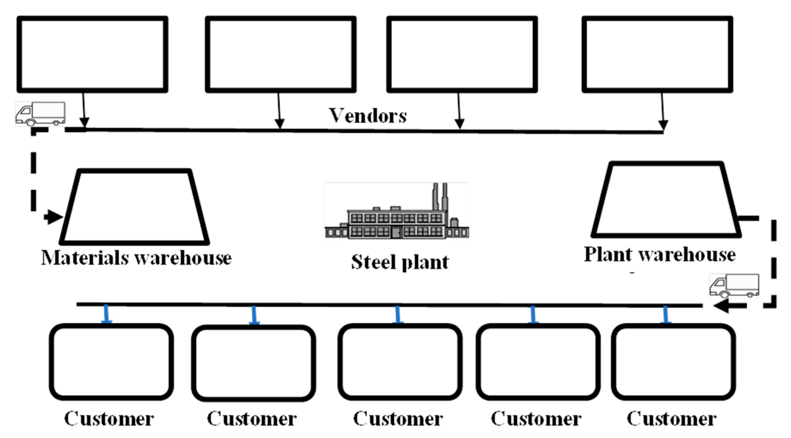
Company S is a medium-sized company (SME) in the Middle East that produces high-quality steel products (e.g., reinforcement and flat bars, angles) by recycling scrap metal, as a primary raw material, using an electric arc furnace. The molten (liquid) steel undergoes rolling and refining operations before being shaped into various types of steel products. Figure 1 depicts the supply chain of company S, which includes a number of vendors, a materials warehouse, a plant warehouse, and a steel plant. Company S sources scrap metal from various local vendors to store it in the warehouse prior to its transfer into the production unit in the steel plant. The end products are stored in a plant warehouse ready for distribution to customers.

This work conceptualizes and proposes an approach that can support the purchasing department throughout the evaluation and selection of the best vendors (suppliers) based on their traditional and resilience performance. We intend to evaluate six key suppliers. Supplier 1 (S1) has 120 employees including permanent and part time. S1’s experience in the metal and steel sector exceeds 15 years. Suppliers S2 and S3 are known as big- and medium-sized holding companies that serve Northern and Southern parts of the country. They have both more than 18 years’ experience and employ 350 workers including engineers, technicians, operators, managers, etc., under a collaborative scheme. Supplier A4 is located in the Eastern part of the country and operates on behalf of a bigger brand in Germany. The company in Germany has more than 450 workers and almost 40 years dedicated to metal and steel production. Supplier A5 has a production plant in the center, that has produced and distributed different types of steel products all around the Middle East for 20 years. Supplier A6 is a global scale exporter owning two assembly and production facilities.

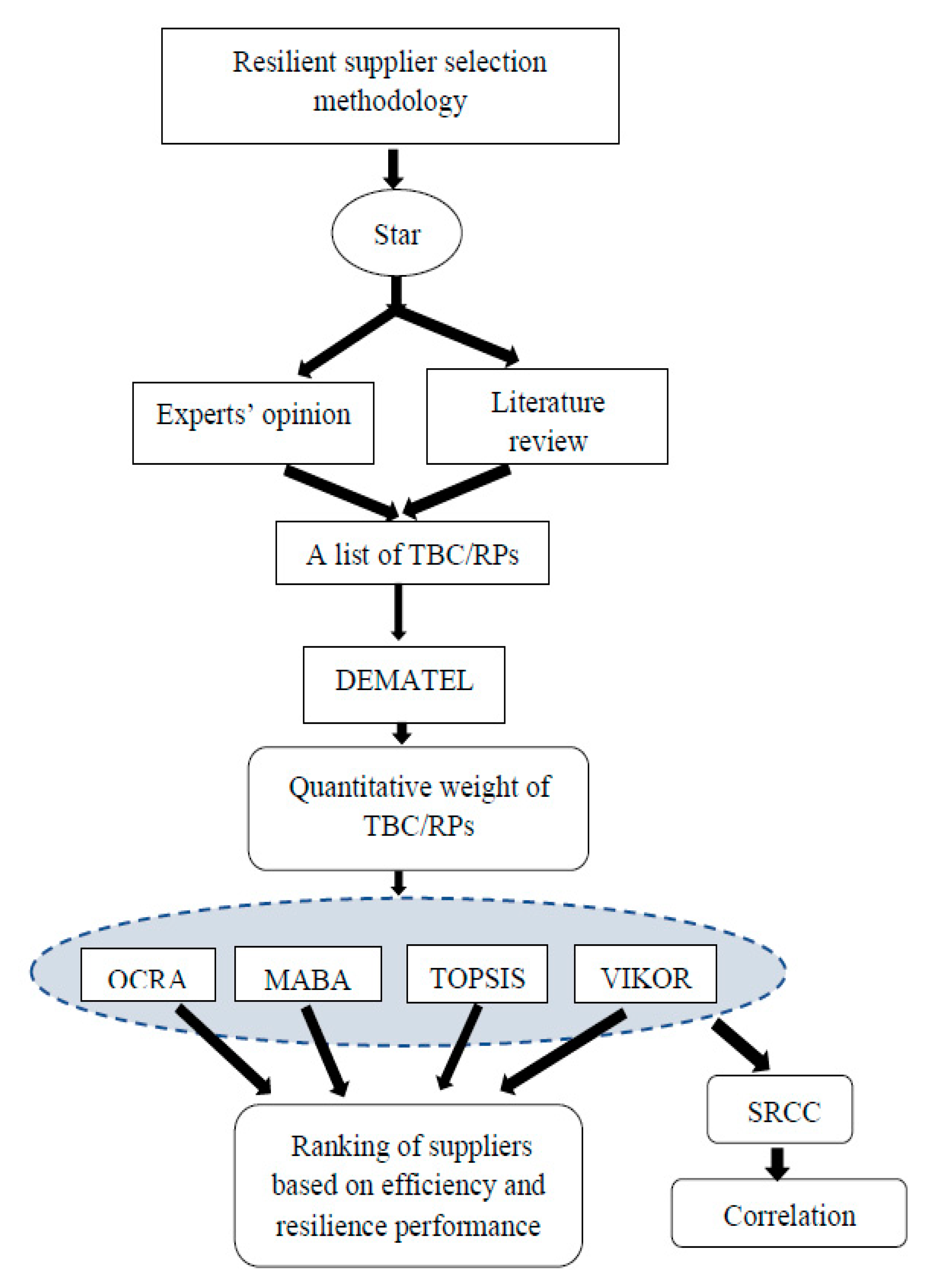
As depicted in Figure 2 and Figure 3, the evaluation of these suppliers is achieved through the following three steps:

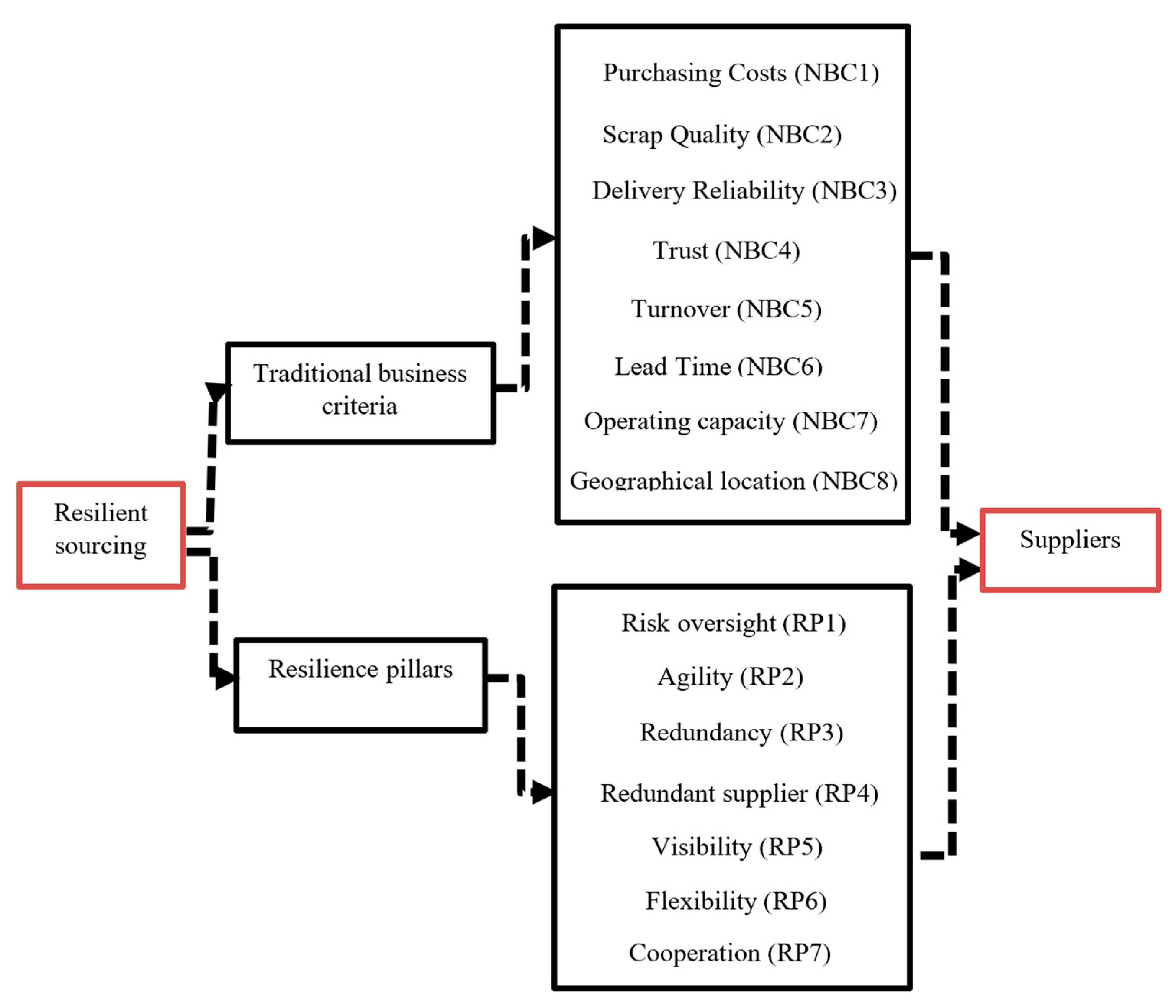
Step 1: Developing a holistic framework that presents the traditional business criteria (TBC) and resilience pillars (RPs) as shown in Figure 2. These TBC/RP are identified based on the review of the literature followed by a filtering with the purchasing team of company S. As shown in Figure 2, TBC include seven criteria: purchasing cost, scrap quality, delivery reliability, lead time, operating capacity, trust, and geographical location. The latter was added by the purchasing department because the company prefers close vendors to reduce the environmental impact.

Step 2: Quantifying the relative importance of TBC/RP shown in Figure 2. This step relies entirely on DMs’ opinions (e.g., purchasing manager and buyers). To this end, the DEMATEL method was applied.

Step 3: Evaluating and selecting the best performing vendors based on TBC/RPs by using the MABAC method. Three other methods, namely OCRA, TOPSIS, and VIKOR, are also applied to validate MABAC’s outcome and prove the rationality of the MCDM methods to the purchasing department.

Step 4: The SRCC method was finally used to explore possible correlation among the four methods.

3.2. DEMATEL: Quantifying the Importance of TBC/RP

The United States Bastille laboratory proposed Decision Making Trial and Evaluation Laboratory (DEMATEL) in 1971. It has been widely used since then to reveal the influence level among criteria. Unlike the AHP method, this technique synthesizes the opinions or experience of experts by quantifying the influence level of each criterion. Through a series of calculations, the DEMATEL results are able to verify the interdependence among all the selected criteria and develop a holistic causes–effects diagram. The application of the DEMATEL method is as follows [86,87]:

Step 1: Generate the direct relation matrix C (Equation (1)) via a pairwise comparison between criteria using the influence scale presented in

Table 3. Influence scale related to DEMATEL.

Linguistic Variable	Scale
No influence (NI)	0
Low influence (LI)	1
Medium influence (MI)	2
High influence (HI)	3
Very high influence (VHI)	4

.

$$\mathrm{C}=\frac{{\mathrm{C}}_1+{\mathrm{C}}_2+\dots +{\mathrm{C}}_{\mathrm{m}}}{\mathrm{m}}=\left[\begin{array}{cccccc}0& c_{12}& \dots & c_{1i}& \dots & c_{1n}\\ c_{21}& 0& \dots & c_{2i}& \dots & c_{2n}\\ \dots & \dots & \dots & \dots & \dots & \dots \\ c_{i1}& \dots & \dots & \dots & \dots & c_{in}\\ \dots & \dots & \dots & \dots & \dots & \dots \\ c_{n1}& c_{n2}& \dots & c_{ni}& \dots & 0\end{array}\right]$$

(1)

where C₁, C₂, and C_m refer to the number of direct relation matrices based on the number of participants (m) in the evaluation of criteria (n).

Step 2: Compute the normalized direct relation matrix N by using Equations (2) and (3).

$$\mathrm{N}=x·\mathrm{C}$$

(2)

where

$$x=min\left[\frac{1}{max{{\displaystyle \sum }}_{i=1}^n{c}_{ij}}, \frac{1}{max{{\displaystyle \sum }}_{j=1}^n{c}_{ij}}\right]\left(i,j=1,2,\dots ,n\right)$$

(3)

Step 3: Generate the total relation matrix T via Equation (4). This matrix depicts the total relationship including direct influence and indirect influence between each pair of criteria.

$$\mathrm{T}=\mathrm{N}{\left(\mathrm{I}-\mathrm{N}\right)}^{-1}$$

(4)

Step 4: Divide the criteria into causes and effects groups by computing the ${\mathrm{D}}_{\mathrm{k}}+{\mathrm{R}}_{\mathrm{k}}$ value called “prominence” and ${\mathrm{D}}_{\mathrm{k}}-{\mathrm{R}}_{\mathrm{k}}$value called “relation” for each criterion. The ${\mathrm{D}}_{\mathrm{k}}$ and ${\mathrm{R}}_{\mathrm{k}}$ are the sums of the rows and the columns of matrix $\left(\mathrm{T}\right),$as presented in Equations (5) and (6), respectively.

$${\mathrm{D}}_i={\displaystyle \sum }_{j=1}^n{t}_{ij}\left(i=1,2,\dots ,n\right)$$

(5)

$${\mathrm{R}}_j={\displaystyle \sum }_{i=1}^n{t}_{ij}\left(j=1,2,\dots ,n\right)$$

(6)

Any criterion would be categorized as (i) a cause when its “relation” value (i.e., ${\mathrm{D}}_{\mathrm{k}}-{\mathrm{R}}_{\mathrm{k}}$) is positive; and (ii) and an effect when its “relation” value is negative.

Step 5: Develop a causes and effects diagram according to the threshold value. The setting of the threshold value $\left(\mathsf{\alpha }\right)$ would be quite helpful for a DM to develop the causes and effects diagram. For example, when the value of total relationship between criterion $i$and criterion j in the matrix $\left(\mathrm{T}\right)$ is greater than the threshold value (i.e., $t_{ij}>\alpha$), it means that criterion $j$ is caused by criterion $i$, where the arrow begins from criterion $i$to criterion $j$ and verse vice. The threshold value $\left(\mathsf{\alpha }\right)$ could be computed by Equation (7), where $num$means the number of elements of the total relation matrix $\left(\mathrm{T}\right)$.

$$\alpha =\frac{1}{N}{\displaystyle \sum }_{i=1}^n{\displaystyle \sum }_{j=1}^m\left[t_{ij}\right]$$

(7)

3.3. MOTV: Evaluation of Supplier Performance

In this work, four MCDM methods are applied to validate the evaluation and the right selection of suppliers.

3.3.1. MABAC

The Multi-Attributive Border Approximation area Comparison (MABAC) method was developed by Pamucar and Cirovic [81]. MABAC is based on ranking an alternative based on its distance of criteria function from the border approximate area. The MABAC is applied as follows [81]:

Step 1. Building the decision matrix D (see Equation (8)) using the evaluation scale presented in

Table 4. Scales used for evaluating resilience performance.

Linguistic Variable	Scale
Very low (VL)	1
Low (L)	3
Medium (M)	5
High (H)	7
Very high (VH)	9

. The DMs hereby need to evaluate vendors vis-à-vis each TBC/RP.

$$\begin{array}{c}D=\frac{{\mathrm{D}}_1+{\mathrm{D}}_2+\dots +{\mathrm{D}}_{\mathrm{k}}}{\mathrm{k}}={\left[d_{ij}\right]}_{nxm}=\left[\begin{array}{cccccc}0& d_{12}& \dots & d_{1i}& \dots & d_{1n}\\ d_{21}& 0& \dots & d_{2i}& \dots & d_{2n}\\ \dots & \dots & \dots & \dots & \dots & \dots \\ d_{i1}& \dots & \dots & \dots & \dots & d_{in}\\ \dots & \dots & \dots & \dots & \dots & \dots \\ d_{m1}& d_{m2}& \dots & d_{mi}& \dots & d_{nm}\end{array}\right]\\ i=1,2,\dots ,m; j=1,2,\dots , n \end{array}$$

(8)

where D₁, D₂, and D_m refer to the number of decision matrices to be built by the number of DMs (k) for the evaluation of criteria (n).

Step 2. Building the normalized decision matrix N_ij as follows:

$$N_{ij}={\left[n_{ij}\right]}_{nxm}; i=1,2,\dots ,m; j=1,2,\dots , n$$

(9)

where elements (n_ij) in Equation (9) can be determined as follows:

For beneficial criteria (e.g., scrap quality),

$$n_{ij}=\frac{d_{ij}-d_i^{-}}{d_i^{+}-d_i^{-}}$$

(10)

For non-beneficial criteria (e.g., purchasing cost),

$$n_{ij}=\frac{d_{ij}-d_i^{+}}{—d_i^{+}}$$

(11)

where $d_i^{+}$= max (x₁, x_2,…, x_m ) and refers to the maximum values of the observed criterion by vendors.

Step 3. Building the weighted normalized decision matrix W_ij as follows:

$$W_{ij}={\left[y_{ij}\right]}_{nxm}; i=1,2,\dots ,m; j=1,2,\dots , n$$

(12)

y_ij = w_j n_ij +w_j, where w_j refers to the criteria weight to be revealed via DEMATEL.

Step 4. Measuring of border approximate area matrix G_ij for each TBC/RP as follows:

$$g_i={\left({\displaystyle \prod }_{j=1}^m{w}_{ij}\right)}^{1/m}$$

(13)

$$G_{ij}=\left[g_1^{j_1} g_2^{j_2} \dots g_n^{j_n} \right]$$

(14)

Step 5. Measuring the distance matrix Q of vendors from the border approximate area (G) as follows:

$$Q=W_{ij}-G_{ij}$$

(15)

Finally, vendors are ranked based on their Q values, in which the highest value refers to the best vendor.

3.3.2. OCRA

The operational competitiveness rating analysis (OCRA) method was developed by Parkan [87]. It is a nonparametric technique that is used to assess the performance of alternatives and productivity analysis. It has been applied in several research studies because of its simplicity and ease of application in addition to its ability to evaluate and diagnose the efficiency of a decision unit over time [88]. The OCRA method is applied as follows [87,88]:

Step 1. Building the decision matrix D as in Equation (16).

$$\begin{array}{l}\mathrm{D}=\frac{{\mathrm{D}}_1+{\mathrm{D}}_2+\dots +{\mathrm{D}}_{\mathrm{k}}}{\mathrm{k}}={\left[d_{ij}\right]}_{nxm}\\ \hspace{1em}\hspace{1em}\hspace{1em}\hspace{1em}=\left[\begin{array}{cccccc}0& d_{12}& \dots & d_{1i}& \dots & d_{1n}\\ d_{21}& 0& \dots & d_{2i}& \dots & d_{2n}\\ \dots & \dots & \dots & \dots & \dots & \dots \\ d_{i1}& \dots & \dots & \dots & \dots & d_{in}\\ \dots & \dots & \dots & \dots & \dots & \dots \\ d_{m1}& d_{m2}& \dots & d_{mi}& \dots & d_{nm}\end{array}\right]\\ \hspace{1em}\hspace{1em}\hspace{1em}i=1,2,\dots ,m; j=1,2,\dots , n \end{array}$$

(16)

where D₁, D₂, and D_m refer to the number of decision matrices to be built by the number of DMs (k) and d_ij refers to the performance of vendor i vis-à-vis criterion j.

Step 2. Determining preference ratings with respect to non-beneficial criteria (e.g., purchasing cost). In this step, only the non-beneficial criteria, which are desired to be minimized, are considered. Equation (17) can be used to calculate the total performance of vendors vis-à-vis non-beneficial criteria as follows:

$${\overline{I}}_i={\displaystyle \sum }_{j=1}^g{w}_j\frac{\max \left(x_{ij}\right)-x_{ij}}{\min \left(x_{ij}\right)}; i=1,2,\dots ,m;j=1,2,\dots , g$$

(17)

${\overline{I}}_i$ corresponding performance of vendor i;

x_ij performance score of vendor i vis-à-vis non-beneficial criteria;

g number of non-beneficial criteria;

w_j relative importance of criterion i.

Step 3. Calculating the total preference rating score for each vendor with respect to non-beneficial criteria, as in Equation (18).

$$\stackrel{\overline{¯}}{I}={\overline{I}}_i+min\left({\overline{I}}_i\right)$$

(18)

where $\stackrel{\overline{¯}}{I}$ refers to the total preference rating score for vendor i with respect to non-beneficial criteria.

Step 4. Determining the preference rating scores vis-à-vis beneficial criteria (e.g., scrap quality) as follows:

$${\overline{O}}_i={\displaystyle \sum }_{j=g+1}^n{w}_j\frac{x_{ij}-\min \left(x_{ij}\right)}{\min \left(x_{ij}\right)}; i=1,2,\dots ,m;j=g+1,g+2,\dots , n$$

(19)

N—g number of beneficial TBC/RP;

w_j—relative weight of beneficial criterion j.

Additionally, it should be noted that the summation of beneficial and non-beneficial criteria weights must equal to one.

Step 5. Calculating the total preference rating score $\left(\stackrel{\overline{¯}}{O}\right)$ for beneficial criteria as follows:

$$\stackrel{\overline{¯}}{O}= {\overline{O}}_i+min\left({\overline{O}}_i\right)$$

(20)

Step 6. Calculating the total preference score P_i for each vendor via Equation (21). The least preferable vendor will take the value of zero.

$$P_i=\left(\stackrel{\overline{¯}}{I}+\stackrel{\overline{¯}}{O}\right)-\min \left(\stackrel{\overline{¯}}{I}+\stackrel{\overline{¯}}{O}\right); i=1,2,\dots ,m$$

(21)

Now, vendors are ranked according to their P_i, where the highest P_i refers to the best vendor performance.

3.3.3. TOPSIS

Hwang and Yoon [89] developed TOPSIS to evaluate alternatives based on their distance from the worst/ideal solutions. Since then, TOPSIS has proved efficient in deriving a ranking of the proposed alternatives [90,91]. In this paper, TOPSIS was adopted to evaluate suppliers’ performance against TBC/RP. TOPSIS was applied as follows [73,87]:

Step 1. Building the decision matrix D (see Equation (22)) using the evaluation scale presented in Table 4.

$$\begin{array}{c}\mathrm{D}=\frac{{\mathrm{D}}_1+{\mathrm{D}}_2+\dots +{\mathrm{D}}_{\mathrm{m}}}{\mathrm{m}}={\left[d_{ij}\right]}_{nxm}=\left[\begin{array}{cccccc}0& d_{12}& \dots & d_{1i}& \dots & d_{1n}\\ d_{21}& 0& \dots & d_{2i}& \dots & d_{2n}\\ \dots & \dots & \dots & \dots & \dots & \dots \\ d_{i1}& \dots & \dots & \dots & \dots & d_{in}\\ \dots & \dots & \dots & \dots & \dots & \dots \\ d_{m1}& d_{m2}& \dots & d_{mi}& \dots & d_{nm}\end{array}\right]\\ i=1,2,\dots ,m; j=1,2,\dots , n \end{array}$$

(22)

where D₁, D₂, and D_m refer to the number of decision matrices to be built by the number of DMs (m) for the evaluation of criteria (n).

Step 2. Building the normalized decision matrix (N) via Equation (23).

$$N_{ij}=\left(\frac{d_{ij}}{\sqrt{{{\displaystyle \sum }}_{i=1}^n{d}_{ij}^2 }}\right); i=1,2,\dots ,m;j=g+1,g+2,\dots , n$$

(23)

Step 3. Multiplying matrix N_ij by criteria weight w_j (derived from DEMATEL) to build the weighted normalized decision matrix W _ij shown in Equation (24).

$$W_{ij}=N_{ij}{w}_j$$

(24)

Step 4. Measuring the distances that the positive and negative ideal solutions are from each criterion for all suppliers by using Equations (25) and (26), respectively.

$${\stackrel{ }{A}}^{+}=\left\{{\stackrel{ }{v}}_1^{+},{\stackrel{}{v}}_2^{+},\mathrm{\dots }{\stackrel{}{,v}}_i^{+}\right\}$$

(25)

$${\stackrel{}{A}}^{-}=\left\{{\stackrel{}{v}}_1^{-},{\stackrel{}{v}}_2^{-},\mathrm{\dots }{\stackrel{}{,v}}_i^{-}\right\}$$

(26)

Step 5. Measuring the distance from the positive ideal solution ($d_i^{+}$) and from the negative ideal solution ($d_i^{-}$) for vendor “i”, as shown in Equation (27).

$$d_i^{+}={\displaystyle \sum _{j\in n}{d}_{}\left(\stackrel{}{v_{ij}},v_j^{+}\right);} d_i^{-}={\displaystyle \sum _{j\in n}{d}_{}\left(\stackrel{}{v_{ij}},v_j^{-}\right);}$$

(27)

where $v_j^{+}$ and $v_j^{-}$refer to the positive/negative ideal points for criterion “j”, respectively.

Step 6. Calculating the closeness coefficient (CC) value for each vendor by using Equation (15). This value represents closeness from the ideal solution and furthermost from the negative solution for each vendor with respect to all TBC/RP.

$$CC=\frac{d_i^{-}}{d_i^{+}+d_i^{-}}$$

(28)

The CC value varies between 1 and 0. The highest CC value refers to the best performance and vice versa.

3.3.4. VIKOR

Serafim Opricovic developed VIKOR as a compromise ranking MADM method [92]. It helps DMs to evaluate and rank alternatives based on their distances from the positive/negative ideal solution [93]. In this paper, VIKOR was adopted to evaluate suppliers’ performance vis-à-vis TBC/RP. VIKOR was applied as follows [92,93]:

Step 1. Building the decision matrix A_ij as shown in Equation (29). Matrix A_ij is built based on decision maker experts using the evaluation scale presented in Table 4.

$$CC=\frac{d_i^{-}}{d_i^{+}+d_i^{-}}$$

(29)

where i and j refer to the suppliers and criteria, respectively.

Step 2. Using Equation (30) to build the normalized decision matrix N_ij.

$$n_{ij}=\frac{r_{ij}}{\left(\sqrt{{\displaystyle \sum _i{r}_{ij}^2}}\right)}$$

(30)

$$w{n}_{ij}=n_{ij}x w_j$$

(31)

Step 3. Using Equation (31) to build the weighted normalized decision matrix W_ij, where w_i is the weight of TBC/RP derived from the DEMATEL method.

Step 4. Using Equations (32) and (33) to measure the positive ideal solution ($f_j^{*}$) and the negative ideal solution ($f_j^{-}$).

$$f_j^{*}=\max w{n}_{ij}$$

(32)

$$f_j^{-}=\min w{n}_{ij}$$

(33)

Step 5. Using Equation (34) to determine the values S_i and R_i as follows:

$$S_I={\displaystyle \sum _{j\in J}^{}{w}_j(f_j^{*}-f_{ij}^{})}/(f_i^{-}-f_i^{})$$

(34)

$$R_i=\underset{j}{\max }{w}_j(f_j^{*}-f_{ij}^{})/(f_i^{-}-f_i^{})$$

(35)

where w_j refers to the weight of TBC/RP derived from DEMATEL, S_i is the distance of the supplier’s performance to the positive ideal solution, and R_i is the maximal regret of each supplier.

Step 6. Using Equation (36) to determine the measuring index Qi.

$$Q_i=v(\frac{S_i-S_{}^{*}}{S^{-}-S_{}^{*}})+(1-v)(\frac{R_i-R_{}^{*}}{R^{-}-R_{}^{*}})$$

(36)

where $S^{*}=\underset{i}{min}{S}_i$ and S* = 0; $S^{-}=\underset{i}{max}{S}_i$ and S- = 1; $R^{*}=\underset{i}{min}{R}_i$ and R* = 0; $R^{-}=\underset{i}{max}{R}_i$ and R- = 1; and v is a weight for the strategy of maximum group utility, whereas 1 v is the weight of the individual regret. Generally, v = 0.5 is assigned when the decision process involves both maximum group utility and individual regret [92].

3.4. SRCC: Exploring Correlation among MOTV

The Spearman rank correlation coefficient (SRCC) approach is used to explore the monotonic association between two sets of data obtained by using two different methods [94,95,96]. Mohammed et al. [83] applied SRCC to investigate the statistical measure between data obtained by ELECTRE and TOPSIS. Chamodrakas et al. [97] applied SRCC to obtain the correlation coefficient between sets of rankings obtained by TOPSIS and a modified version of TOPSIS. Similar studies were presented by [98,99,100]. In this research, the SRCC approach was proposed to explore the degree of correlation among MOTV that reveal four rankings of suppliers as follows:

$$SRCC=1-\frac{6{{\displaystyle \sum }}_{i=1}^m{y}_i^2 }{X^3-x}; -1\le SRCC\le 1$$

(37)

where the SRCC value refers to the correlation level among the four rankings obtained by using MOTV; x is the number of suppliers; X is the total number of suppliers; and y is the difference between two considered rankings. Thus, this approach is applied several times to reveal the correlation value between two evaluation methods at a time.

The correlation value (SRCC) varies between −1.0 (an absolute negative correlation) and 1.0 (an absolute positive correlation). Accordingly, it can be, verbally, categorized as follows:

• 1 🡲 “absolute”;
• 0.8–0.999 🡲 “very strong”;
• 0.6–0.79 🡲 “strong”;
• 0.4–0.59 🡲 “moderate”;
• 0.2–0.39 🡲 “weak”;
• SRCC < 0.19 🡲 “very weak”.

4. The D-MOTV Approach: Results and Discussion

In this case study, we have designed, in collaboration with the purchasing manager, a group decision-making platform involving five experts of various knowledge and experience backgrounds from the purchasing department. These include:

• The purchasing manager who has been working in the procurement field for 20 years;
• Two senior buyers with an average of 8 years’ experience in the purchasing department;
• A buyer with 3 years’ experience in production and purchasing;
• 1A junior buyer who joined the company 8 months ago (from the date of data collection).

These employees were met with twice: (1) as a group to discuss the methodology and its application steps and required data, and (2) individually to collect the required data. These meetings were held online and lasted around 1.5 h.

4.1. Quantifying Criteria: DEMATEL

In this section, we adopt the DEMATEL tool. This is a method that generally computes the weights of the decision factors and explores their influence, categorizing them into cause and effect groups. We have defined RP as per each resilience pillar, including Flexibility, Redundancy, Agility, Redundant supplier, Risk oversight, Cooperation, and Visibility. The complete list of criteria is available in

Table 5. Definitions of TBC/RP.

TBC/RP		Definition
TBC	Purchasing cost (TBC1)	Compare purchase cost per unit among alternatives
	Scrap quality (TBC2)	Contents of iron (as the main component) and non-ferrous admixtures
	Delivery Reliability (TBC3)	The ability to conform with a promised scheduled delivery plan consistently
	Trust (TBC4)	The gauge of positive historical collaborations
	Turnover (TBC5)	Vendors’ capability to satisfy company’s needs
	Lead Time (TBC6)	The duration of time from putting an order in to the receipt of the order
	Operating capacity (TBC7)	The asset within which a company hopes to operate—commonly during a short-term period
	Geographical location (TBC8)	The distance from a vendor’s location to Company S’ location
RP	Flexibility (RP1)	Vendors’ ability to react smoothly to turbulences in the supply chain with respect to similar costs and lead times.
	Redundancy (RP2)	Vendors’ ability to absorb disruptions to materials within the supply chain via redundant suppliers
	Agility (RP3)	Vendors’ ability to respond quickly and efficiently to reasonably small business opportunities in collaboration with a collaborator able to cope with unanticipated/unpredictable demand
	Redundant supplier (RP4)	Vendors’ ability and willingness to collaborate with a new supplier to absorbs disruptions to materials within the supply chain
	Risk oversight (RP5)	Vendors’ ability to stay tuned to potential disruptions outside its company
	Cooperation (RP6)	Vendors’ willingness to keep cooperation with their clients to develop proactive and reactive plans towards resilience business
	Visibility (RP7)	Vendors’ willingness to share relevant information with their clients; this helps both parties to see the light at the end of the resilience tunnel

. The aggregated ratings for pairs of criteria are shown in

Table 6. The aggregated decision matrix for RP.

Pillars	RP1	RP2	RP3	RP4	RP5	RP6	RP7
RP1	0	2	4	3	0	4	4
RP2	4	0	1	0	0	0	0
RP3	4	4	0	0	0	0	0
RP4	4	3	3	0	3	4	1
RP5	4	4	2	4	0	0	4
RP6	2	0	0	0	4	0	4
RP7	2	4	3	0	1	4	0

, which is obtained by Equation (1) as a reflection of the general form of the decision matrix called the direct relation matrix. The normalized direct relation matrix for RP, given in

Table 7. The aggregated normalized decision matrix for RP.

Pillars	RP1		RP2	RP3	RP4	RP5	RP6	RP7
RP1	0		0.1	0.2	0.15	0	0.2	0.2
RP2	0.2		0	0.05	0	0	0	0
RP3	0.2		0.2	0	0	0	0	0
RP4	0.2		0.15	0.15	0	0.15	0.2	0.05
RP5	0.2		0.2	0.1	0.2	0	0	0.2
RP6	0.1		0	0	0	0.2	0	0.2
RP7	0.1		0.2	0.15	0	0.05	0.2	0

, is worked out through Equations (2) and (3). The next step is to obtain the total relation matrix (T) that must be achieved using Equation (4). We performed the (T) matrix and

Table 8. The total influence matrix (T) for RP ($t_{ij}^{*}>0.2346$).

Pillars	RP1	RP2	RP3	RP4	RP5	RP6	RP7
RP1	0285*	0.335*	0.374*	0.218	0.126	0.374*	0.368*
RP2	0.273*	0.081	0.130	0.046	0.027	0.079	0.078
RP3	0.311*	0.283*	0.101	0.053	0.031	0.091	0.089
RP4	0.494*	0.398*	0.356*	0.126	0.259*	0.381*	0.283*
RP5	0.504*	0.462*	0.338*	0.298*	0.111	0.238	0.386*
RP6	0.292*	0.197	0.160	0.096	0.261*	0.147	0.345*
RP7	0.313*	0.355*	0.277*	0.073	0.130	0.308*	0.154

releases the corresponding data. According to this table, the sum of each row and column results in two vectors called D and R, respectively. The vectors are computed using Equation (5).

Table 9. Total influence and net influence levels for RP.

Pillars	D	R	D+R	D-R	Weights	Group
RP1	2.079	2.472	4.551	−0.393	0.197999	effect
RP2	0.714	2.110	2.824	−1.397	0.122863	effect
RP3	0.959	1.736	2.695	−0.778	0.11725	effect
RP4	2.297	0.910	3.207	1.387	0.139526	cause
RP5	2.336	0.945	3.281	1.391	0.142745	cause
RP6	1.497	1.617	3.114	−0.120	0.13548	effect
RP7	1.611	1.702	3.313	−0.092	0.144137	effect

offers evidence for this step. The information provided represents (D + R) and (D – R), which are the degree of total influence levels and the degree of net influence levels, respectively. Indeed, the positive values claim that it will influence the other requirements more than any other requirement influences it. The two categories of Cause and Effect are presented in Table 9. Based on the results, it appears that RP1 and RP3 are the most effective and least important factors produced by DEMATEL, respectively. The threshold value computed by Equation (7) is marked (*) in Table 8; this states the interaction between the criteria. For example, in the case of RP1 and RP2, the corresponding value is 0.335, which is higher than 0.2346. This means that RP2 is affected by RP1. This can be very important for DMs for further analysis of the decision environment. It must be mentioned that RP4 and RP5 are placed in the cause group, while the rest of the pillars are classified as effects.

In the second level for DEMATEL computation, we followed a similar procedure. We assumed that the Traditional Business criteria (TBC) include Purchasing cost (TBC1), Scrap Quality (TBC2), Delivery reliability (TBC3), Trust (TBC4), Turnover (TBC5), Lead time (TBC6), Operating capacity (TBC7), and Geographical location (TBC8). Similar to the previous calculations, the aggregated opinion of experts for TBC is observable in

Table 10. The aggregated decision matrix for TBC.

Criteria	TBC1	TBC2	TBC3	TBC4	TBC5	TBC6	TBC7	TBC8
TBC1	0	4	2	1	1	2	0	0
TBC2	4	0	3	4	2	2	0	0
TBC3	0	1	0	4	0	4	0	1
TBC4	4	1	1	0	0	4	0	0
TBC5	2	2	0	2	0	0	4	0
TBC6	0	0	1	4	0	0	1	0
TBC7	4	0	0	4	2	0	0	0
TBC8	3	0	3	0	0	3	0	0

. Next, it is necessary to release the normalized decision (

Table 11. The normalized decision matrix for TBC.

Criteria	TBC1	TBC2	TBC3	TBC4	TBC5	TBC6	TBC7	TBC8
TBC1	0	0.211	0.105	0.053	0.053	0.105	0	0
TBC2	0.211	0	0.158	0.211	0.105	0.105	0	0
TBC3	0	0.053	0	0.211	0	0.211	0	0.053
TBC4	0.211	0.053	0.053	0	0	0.211	0	0
TBC5	0.105	0.105	0	0.105	0	0	0.211	0
TBC6	0	0	0.053	0.211	0	0	0.053	0
TBC7	0.211	0	0	0.211	0.105	0	0	10
TBC8	0.158	0	0.158	0	0	0.158	0	0

).

To compute the total influence matrix for TBC based on DEMATEL formulation, we used Equation (4) and the results are given in

Table 12. The total influence matrix (T) for TBC.

Criteria	TBC1	TBC2	TBC3	TBC4	TBC5	TBC6	TBC7	TBC8
TBC1	0.120	0.267	0.185	0.219	0.090	0.233	0.031	0.010
TBC2	0.345	0.121	0.252	0.393	0.141	0.292	0.045	0.013
TBC3	0.104	0.097	0.069	0.326	0.018	0.324	0.021	0.056
TBC4	0.276	0.128	0.127	0.142	0.030	0.311	0.023	0.007
TBC5	0.251	0.181	0.075	0.250	0.056	0.115	0.228	0.004
TBC6	0.081	0.037	0.087	0.274	0.015	0.089	0.060	0.005
TBC7	0.320	0.102	0.074	0.313	0.137	0.126	0.035	0.004
TBC8	0.206	0.063	0.212	0.129	0.019	0.260	0.018	0.011

. This matrix declares how the total relation of factors was realized by the expert’s attitude. For the next step of DEMATEL, we sum each row and each column of Table 12 to build the new decision (

Table 13. Total influence and net influence levels for TBC.

Criteria	Di	Ri	Di+Ri	Di-Ri	Group	Weights
TBC1	1.1547	1.7032	2.8580	−0.5485	effect	0.165
TBC2	1.6028	0.9975	2.6003	0.6053	cause	0.150
TBC3	1.0150	1.0801	2.0951	−0.0651	effect	0.121
TBC4	1.0435	2.0458	3.0893	−1.0023	cause	0.178
TBC5	1.1604	0.5064	1.6668	0.6540	effect	0.096
TBC6	0.6474	1.7491	2.3965	−1.1018	cause	0.138
TBC7	1.1112	0.4618	1.5731	0.6494	effect	0.091
TBC8	0.9185	0.1095	1.0280	0.8090	effect	0.059

). In this group of criteria, TBC4 (trust) is named as the best criterion while TBC8 is identified as the least important. In addition, five criteria belong to the effects group and there are three cause-related criteria.

The complete list of 15 evaluation factors is presented in

Table 14. Weight of TBC/RP via DEMATEL.

Aspect	Criteria/Pillars	Weight	Ranking
TBC	TBC1	0.1651	2
	TBC2	0.1502	3
	TBC3	0.1211	5
	TBC4	0.1785	1
	TBC5	0.0963	6
	TBC6	0.1385	4
	TBC7	0.0909	7
	TBC8	0.0594	8
RP	RP1	0.1980	1
	RP2	0.1230	6
	RP3	0.1170	7
	RP4	0.1400	4
	RP5	0.1430	3
	RP6	0.1350	5
	RP7	0.1440	2

. We used the data of this table for the main decision matrix where the ranking-based methods are directed to supplier performance assessment.

4.2. Comparing the Performance of Suppliers (MOTV)

This section is devoted to evaluating and selecting the best vendors (suppliers) based on TBC/RP using the MABAC and analytical comparison to OCRA, TOPSIS, and VIKOR. In this way, we can examine the applicability of the different MCDM methods and deliver the results to the purchasing department.

4.2.1. MABAC

The first ranking method is MABAC, as in Section 3.3.1. As mentioned, the primary matrix is formed using Equation (8). Then, the normalized decision matrix in

Table 15. Results related to MABAC application.

Normalized DM
	TBC1	TBC2	TBC3	TBC4	TBC5	TBC6	TBC7	TBC8	RP1	RP2	RP3	RP4	RP5	RP6	RP7
S1	1	1	0.50	0.83	0	0.25	0.50	0.50	1	0.33	1	1	1	0.83	1
S2	0.73	1	0	0	0	0	0	1	0.50	0	0	0	0.50	0.33	0
S3	0.73	0	0	0.50	1	0.50	0	0	0	0.33	0.33	0	0	0	0.33
S4	0.36	1	0.50	1	0	1	0	0.50	1	1	1	0.50	0.50	1	0.67
S5	0.73	0	0	0.33	0	0.50	1	1	0	0.33	0.33	0	0.50	0.67	0.67
S6	0	1	1	1	0	0.50	0.50	0.75	1	0.67	0.67	0.25	0.50	0.83	0.83
Weight normalized DM
	TBC1	TBC2	TBC3	TBC4	TBC5	TBC6	TBC7	TBC8	RP1	RP2	RP3	RP4	RP5	RP6	RP7
S1	0.33	0.30	0.18	0.33	0.10	0.17	0.14	0.09	0.40	0.16	0.23	0.28	0.29	0.25	0.29
S2	0.29	0.30	0.12	0.18	0.10	0.14	0.09	0.12	0.30	0.12	0.12	0.14	0.21	0.18	0.14
S3	0.29	0.15	0.12	0.27	0.19	0.21	0.09	0.06	0.20	0.16	0.16	0.14	0.14	0.14	0.19
S4	0.23	0.30	0.18	0.36	0.10	0.28	0.09	0.09	0.40	0.25	0.23	0.21	0.21	0.27	0.24
S5	0.29	0.15	0.12	0.24	0.10	0.21	0.18	0.12	0.20	0.16	0.16	0.14	0.21	0.23	0.24
S6	0.17	0.30	0.24	0.36	0.10	0.21	0.14	0.10	0.40	0.20	0.20	0.17	0.21	0.25	0.26
G	0.26	0.24	0.16	0.28	0.11	0.20	0.12	0.09	0.30	0.17	0.18	0.17	0.21	0.21	0.22
Distance from Q
	TBC1	TBC2	TBC3	TBC4	TBC5	TBC6	TBC7	TBC8	RP1	RP2	RP3	RP4	RP5	RP6	RP7
S1	0.07	0.06	0.03	0.05	−0.01	−0.02	0.02	0	0.10	−0.01	0.06	0.11	0.08	0.04	0.07
S2	0.03	0.06	−0.03	−0.10	−0.01	−0.06	−0.03	0.02	0	−0.05	−0.06	−0.03	0	−0.03	−0.08
S3	0.03	−0.09	−0.03	−0.01	0.08	0.01	−0.03	−0.03	−0.10	−0.01	−0.02	−0.03	−0.07	−0.08	−0.03
S4	−0.03	0.06	0.03	0.08	−0.01	0.08	−0.03	0	0.10	0.07	0.06	0.04	0	0.06	0.02
S5	0.03	−0.09	−0.03	−0.04	−0.01	0.01	0.06	0.02	−0.10	−0.01	−0.02	−0.03	0	0.01	0.02
S6	−0.09	0.06	0.09	0.08	−0.01	0.01	0.02	0.01	0.10	0.03	0.02	0	0	0.04	0.04
G	0.07	0.06	0.03	0.05	−0.01	−0.02	0.02	0	0.10	−0.01	0.06	0.11	0.08	0.04	0.07

is obtained by Equations (9)–(11). The weighted normalized matrix and the distance measures from Q values are also shown in Table 15. The weighted normalized matrix and the distance Q from the border approximate area are computed using Equations (12) and (15), respectively. The higher the Q values, the better the ranking, as shown in

Table 16. Q value for the six suppliers related to MABAC.

Supplier	Q
S1	0.6144
S2	−0.3702
S3	−0.4125
S4	0.5128
S5	−0.1785
S6	0.3909

. Based on the results of the MABAC, supplier S1 is selected as the best option.

4.2.2. OCRA

OCRA is the next method used to evaluate the vendors’ performances. Using Equations (17)–(20), we compute the preference ratings with respect to beneficial and non-beneficial criteria, as shown in

Table 17. Results related to OCRA application.

Preference Ratings with respect to non-Beneficial Criteria
	TBC1	TBC2	TBC3	TBC4	TBC5	TBC6	TBC7	TBC8	RP1	RP2	RP3	RP4	RP5	RP6	RP7
S1	0.26	0	0	0	0	0	0	0	0	0	0	0	0	0	0
S2	0.19	0	0	0	0	0	0	0	0	0	0	0	0	0	0
S3	0.19	0	0	0	0	0	0	0	0	0	0	0	0	0	0
S4	0.09	0	0	0	0	0	0	0	0	0	0	0	0	0	0
S5	0.19	0	0	0	0	0	0	0	0	0	0	0	0	0	0
S6	0	0	0	0	0	0	0	0	0	0	0	0	0	0	0
Preference Ratings with respect to Beneficial Criteria
	TBC1	TBC2	TBC3	TBC4	TBC5	TBC6	TBC7	TBC8	RP1	RP2	RP3	RP4	RP5	RP6	RP7
S1	0	0.06	0.05	0.30	0	0.03	0.04	0.04	0.26	0.08	0.09	1.12	0.57	0.23	0.29
S2	0	0.06	0	0	0	0	0	0.08	0.13	0	0	0	0.29	0.09	0
S3	0	0	0	0.18	0.02	0.06	0	0	0	0.08	0.03	0	0	0	0.10
S4	0	0.06	0.05	0.36	0	0.11	0	0.04	0.26	0.25	0.09	0.56	0.29	0.27	0.19
S5	0	0	0	0.12	0	0.06	0.07	0.08	0	0.08	0.03	0	0.29	0.18	0.19
S6	0	0.06	0.10	0.36	0	0.06	0.04	0.06	0.26	0.16	0.06	0.28	0.29	0.23	0.24

. Next, we use Equation (21) to evaluate the overall preference for each supplier and identify the list of preferred suppliers. As shown in

Table 18. Overall Preference (P) for the six suppliers related to OCRA.

Supplier	$\overline{\mathrm{I}}$	$\stackrel{\overline{¯}}{\mathrm{I}}$	$\overline{\mathrm{O}}$	$\stackrel{\overline{¯}}{\mathrm{O}}$	$\stackrel{\overline{¯}}{\mathrm{I}}+\stackrel{\overline{¯}}{\mathrm{O}}$	Overall Preference (P)
S1	0.259	0.259	3.145	2.684	2.944	2.755
S2	0.189	0.189	0.647	0.187	0.375	0.187
S3	0.189	0.189	0.46	0	0.189	0
S4	0.094	0.094	2.52	2.06	2.154	1.965
S5	0.189	0.189	1.096	0.635	0.824	0.635
S6	0	0	2.182	1.722	1.722	1.533

, the results reveal that OCRA, like MABAC, selects S1 as the best supplier.

4.2.3. TOPSIS

TOPSIS is amongst the most applied decision-making tools with multiple variables. On hand, the decision matrices reflecting the suppliers and relevant factors, Equations (23) and (24), are used to produce, respectively, the normalized and the weighted normalized matrices for suppliers’ evaluation, as shown in

Table 19. Results related to TOPSIS application.

TOPSIS Performance Rating
	TBC1	TBC2	TBC3	TBC4	TBC5	TBC6	TBC7	TBC8	RP1	RP2	RP3	RP4	RP5	RP6	RP7
S1	3.5	7	7	8	5	6	7	5	7	5	7	9	5	8	9
S2	5	7	5	3	5	5	5	7	5	3	4	1	3	5	3
S3	5	5	5	6	6	7	5	3	3	5	5	1	1	3	5
S4	7	7	7	9	5	9	5	5	7	9	7	5	3	9	7
S5	5	5	5	5	5	7	9	7	3	5	5	1	3	7	7
S6	9	7	9	9	5	7	7	6	7	7	6	3	3	8	8
Normalized DM
	TBC1	TBC2	TBC3	TBC4	TBC5	TBC6	TBC7	TBC8	RP1	RP2	RP3	RP4	RP5	RP6	RP7
S1	0.60	1.14	1.14	1.26	0.90	0.94	1.14	0.87	1.24	0.86	1.2	2.01	1.18	1.26	1.44
S2	0.85	1.14	0.81	0.47	0.9	0.78	0.81	1.22	0.88	0.51	0.69	0.22	0.71	0.79	0.48
S3	0.85	0.81	0.81	0.95	1.08	1.09	0.81	0.52	0.53	0.86	0.86	0.22	0.24	0.47	0.8
S4	1.19	1.14	1.14	1.42	0.9	1.41	0.81	0.87	1.24	1.54	1.2	1.12	0.71	1.42	1.12
S5	0.85	0.81	0.81	0.79	0.9	1.09	1.46	1.22	0.53	0.86	0.86	0.22	0.71	1.11	1.12
S6	1.53	1.14	1.46	1.42	0.9	1.09	1.14	1.04	1.24	1.20	1.03	0.67	0.71	1.26	1.28
Weight normalized DM
	TBC1	TBC2	TBC3	TBC4	TBC5	TBC6	TBC7	TBC8	RP1	RP2	RP3	RP4	RP5	RP6	RP7
S1	0.1	0.17	0.14	0.23	0.09	0.13	0.1	0.05	0.25	0.11	0.14	0.28	0.17	0.17	0.21
S2	0.14	0.17	0.1	0.08	0.09	0.11	0.07	0.07	0.18	0.06	0.08	0.03	0.10	0.11	0.07
S3	0.14	0.12	0.1	0.17	0.1	0.15	0.07	0.03	0.11	0.11	0.10	0.03	0.03	0.06	0.12
S4	0.20	0.17	0.14	0.25	0.09	0.19	0.07	0.05	0.25	0.19	0.14	0.16	0.10	0.19	0.16
S5	0.14	0.12	0.1	0.14	0.09	0.15	0.13	0.07	0.11	0.11	0.10	0.03	0.10	0.15	0.16
S6	0.25	0.17	0.18	0.25	0.09	0.15	0.1	0.06	0.25	0.15	0.12	0.09	0.10	0.17	0.18
Distance to ideal
	TBC1	TBC2	TBC3	TBC4	TBC5	TBC6	TBC7	TBC8	RP1	RP2	RP3	RP4	RP5	RP6	RP7
S1	0.15	0	0.04	0.03	0.02	0.06	0.03	0.02	0	0.08	0	0	0	0.02	0
S2	0.11	0	0.08	0.17	0.02	0.09	0.06	0	0.07	0.13	0.06	0.25	0.07	0.09	0.14
S3	0.11	0.05	0.08	0.08	0	0.04	0.06	0.04	0.14	0.08	0.04	0.25	0.13	0.13	0.09
S4	0.06	0	0.04	0	0.02	0	0.06	0.02	0	0	0	0.12	0.07	0	0.05
S5	0.11	0.05	0.08	0.11	0.02	0.04	0	0	0.14	0.08	0.04	0.25	0.07	0.04	0.05
S6	0	0	0	0	0.02	0.04	0.03	0.01	0	0.04	0.02	0.19	0.07	0.02	0.02
Distance to worst
	TBC1	TBC2	TBC3	TBC4	TBC5	TBC6	TBC7	TBC8	RP1	RP2	RP3	RP4	RP5	RP6	RP7
S1	0	0.05	0.04	0.14	0	0.02	0.03	0.02	0.14	0.04	0.06	0.25	0.13	0.11	0.14
S2	0.04	0.05	0	0	0	0	0	0.04	0.07	0	0	0	0.07	0.04	0
S3	0.04	0	0	0.08	0.02	0.04	0	0	0	0.04	0.02	0	0	0	0.05
S4	0.10	0.05	0.04	0.17	0	0.09	0	0.02	0.14	0.13	0.06	0.12	0.07	0.13	0.09
S5	0.04	0	0	0.06	0	0.04	0.06	0.04	0	0.04	0.02	0	0.07	0.09	0.09
S6	0.15	0.05	0.08	0.17	0	0.04	0.03	0.03	0.14	0.08	0.04	0.06	0.07	0.11	0.12

. Once the ideal and the non-ideal solutions are identified, the distances to the best (ideal) and the worst solutions are found. The maximum distances from the worst solution and the minimum distances from the best solution are reported in

Table 20. TOPSIS closeness coefficient values for the six suppliers.

Supplier	Di+	Di-	CC
S1	0.199	0.402	0.669
S2	0.420	0.131	0.237
S3	0.411	0.124	0.232
S4	0.176	0.367	0.675
S5	0.368	0.186	0.336
S6	0.214	0.355	0.624

along with the corresponding closeness coefficient measure of each supplier. The latter results indicate that TOPSIS elects S4 as the best supplier and S1 as the second-best.

4.2.4. VIKOR

The application of VIKOR requires the calculating of the normalized and weighted normalized matrices using Equations (30) and (31), respectively, followed by the positive and negative ideal solutions, which are obtained via Equations (32) and (33), respectively. The results are presented in

Table 21. Results related to VIKOR application.

Normalized DM
	TBC1	TBC2	TBC3	TBC4	TBC5	TBC6	TBC7	TBC8	RP1	RP2	RP3	RP4	RP5	RP6	RP7
S1	0.24	0.45	0.44	0.46	0.39	0.35	0.44	0.36	0.51	0.34	0.49	0.83	0.64	0.47	0.54
S2	0.34	0.45	0.31	0.17	0.39	0.29	0.31	0.50	0.36	0.21	0.28	0.09	0.38	0.29	0.18
S3	0.34	0.32	0.31	0.35	0.47	0.41	0.31	0.22	0.22	0.34	0.35	0.09	0.13	0.18	0.30
S4	0.47	0.45	0.44	0.52	0.39	0.53	0.31	0.36	0.51	0.62	0.49	0.46	0.38	0.53	0.42
S5	0.34	0.32	0.31	0.29	0.39	0.41	0.56	0.50	0.22	0.34	0.35	0.09	0.38	0.41	0.42
S6	0.61	0.45	0.56	0.52	0.39	0.41	0.44	0.43	0.51	0.48	0.42	0.28	0.38	0.47	0.48
Weighted normalized DM
	TBC1	TBC2	TBC3	TBC4	TBC5	TBC6	TBC7	TBC8	RP1	RP2	RP3	RP4	RP5	RP6	RP7
S1	0.04	0.07	0.05	0.08	0.04	0.05	0.04	0.02	0.10	0.04	0.06	0.12	0.09	0.06	0.08
S2	0.06	0.07	0.04	0.03	0.04	0.04	0.03	0.03	0.07	0.03	0.03	0.01	0.05	0.04	0.03
S3	0.06	0.05	0.04	0.06	0.05	0.06	0.03	0.01	0.04	0.04	0.04	0.01	0.02	0.02	0.04
S4	0.08	0.07	0.05	0.09	0.04	0.07	0.03	0.02	0.10	0.08	0.06	0.06	0.05	0.07	0.06
S5	0.06	0.05	0.04	0.05	0.04	0.06	0.05	0.03	0.04	0.04	0.04	0.01	0.05	0.06	0.06
S6	0.10	0.07	0.07	0.09	0.04	0.06	0.04	0.03	0.10	0.06	0.05	0.04	0.05	0.06	0.07
Values of w*(((f+)-fij)/(f+)-(f-))
	TBC1	TBC2	TBC3	TBC4	TBC5	TBC6	TBC7	TBC8	RP1	RP2	RP3	RP4	RP5	RP6	RP7
S1	0	0	0.06	0.03	0.10	0.10	0.05	0.03	0	0.08	0	0	0	0.02	0
S2	0.05	0	0.12	0.18	0.10	0.14	0.09	0	0.10	0.12	0.12	0.14	0.07	0.09	0.14
S3	0.05	0.15	0.12	0.09	0	0.07	0.09	0.06	0.20	0.08	0.08	0.14	0.14	0.14	0.10
S4	0.11	0	0.06	0	0.10	0	0.09	0.03	0	0	0	0.07	0.07	0	0.05
S5	0.05	0.15	0.12	0.12	0.10	0.07	0	0	0.20	0.08	0.08	0.14	0.07	0.05	0.05
S6	0.17	0	0	0	0.10	0.07	0.05	0.01	0	0.04	0.04	0.10	0.07	0.02	0.02

. Next, the distance of the supplier’s performance to the positive ideal solution S_i and the maximal regret of each supplier R_i are computed through Equations (34) and (35). The corresponding results are shown in

Table 22. S_i, R_i, and Q_i values for the six suppliers related to VIKOR.

Supplier	Si	Ri	Qi	Weight (Si+Ri+Qi) (between 0 and 3)
S1	0.4701	0.1039	0	0.5739
S2	1.4547	0.1785	0.8758	2.5090
S3	1.4970	0.1980	1	2.6950
S4	0.5717	0.1051	0.0560	0.7328
S5	1.2631	0.1980	0.8861	2.3472
S6	0.6936	0.1651	0.4342	1.2930

. VIKOR claims that S1 is the best supplier among other candidates, which supports the results of OCRA and MABAC.

Table 23. Ranking of suppliers via MOTV.

Supplier	MABAC	OCRA	TOPSIS	VIKOR
S1	1	1	2	1
S2	5	5	5	5
S3	6	6	6	6
S4	2	2	1	2
S5	4	4	4	4
S6	3	3	3	3

confirms the stability of the proposed case study and its computational accuracy.

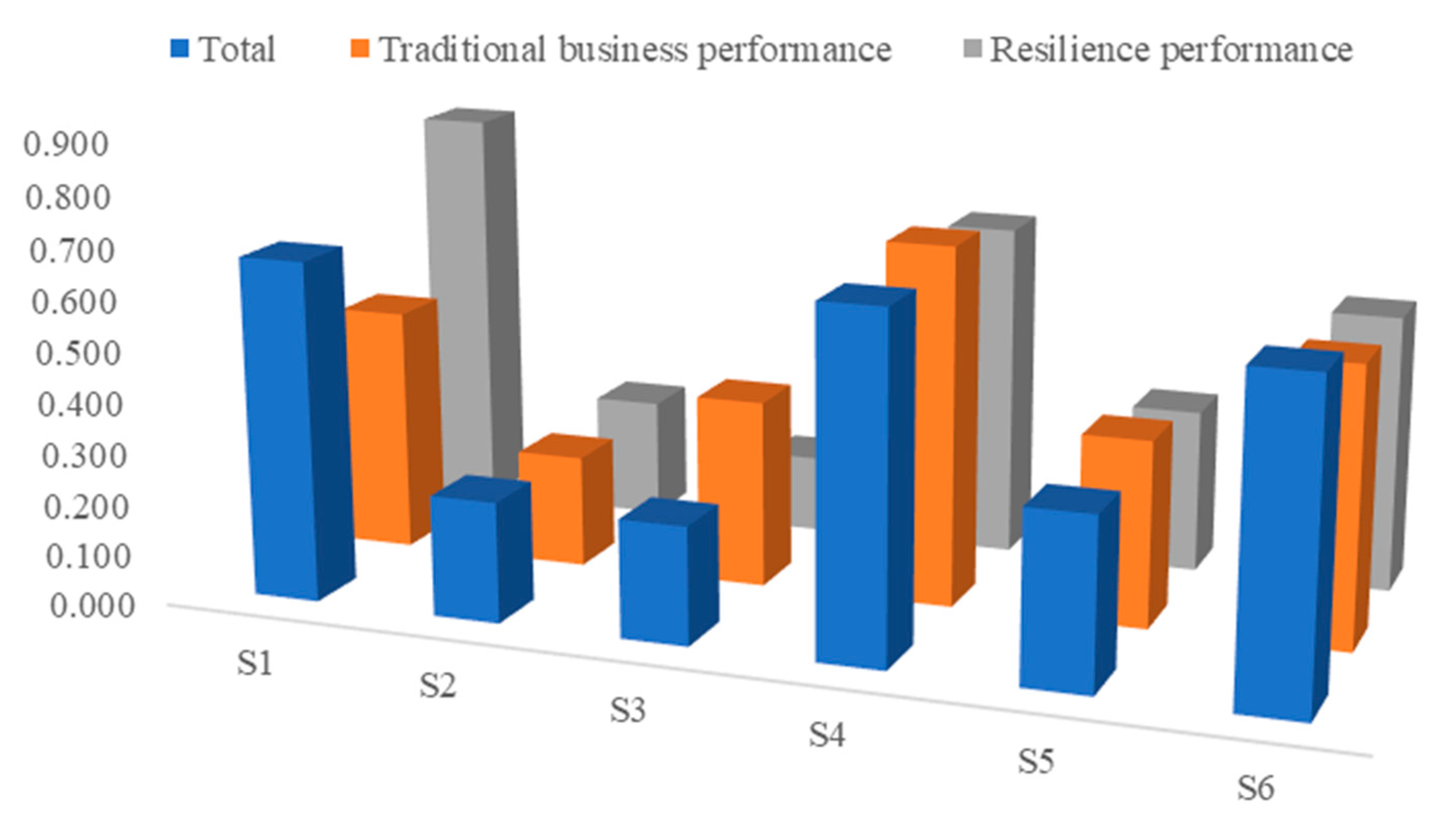
Figure 4 depicts the supplier’s performance vis-à-vis resilience, traditional, and resilience/traditional criteria individually, as reflected through TOPSIS. Hence, in terms of resilience dimensions, S1 is presented as the best supplier, followed by S4 and S6. As such, the initial experts’ evaluation (see Table 20) showed partial, low traditional performance, mainly for purchasing cost, turnover, and geographical location. Thus, these factors might hurdle their way towards superiority vis-à-vis the traditional aspects. Meanwhile, it is observed that S3 is the worst supplier with regard to the resilience approach, whereas S4 is the best from the traditional business performance perspective. Therefore, it appears that despite performing pretty well under traditional or resilience evaluations, some suppliers may fail to be the best when considering both aspects.

The last stage of the suppliers’ performance evaluation consists of comparing the outcomes of the four methods using SRCC. The results in

Table 24. Correlation type among MOTV.

MCDM Method	SRCC Equation	SRCC Value	Correlation Type
TOPSIS and OCRA, VIKOR or MABAC	$1-\frac{6\ast 2}{{(6)}^3-6}$	$0.942$	Very strong
Among OCRA, VIKOR and MABAC	$1-\frac{6\ast 0}{{(6)}^3-0}$	1	Absolute

reveal an absolute correlation between OCRA, VIKOR, and MABAC, which produce the same rankings, as shown earlier.

On the other hand, there is a strong correlation between TOPSIS and any of the latter techniques due certainly to the fact that TOPSIS swaps the rank positions of the best and the next best suppliers, in spite of a total agreement on the overall ranking.

4.3. Managerial Implications

The research outcome of the proposed D-MOTV approach helped DMs in the purchasing department to easily evaluate and rank suppliers’ performance. This research can support supply chain managers in building resilient supply chains that reduce not only sourcing costs, but also potential losses due to disruption threats. Furthermore, the D-MOTV approach can be used as a guide to diagnose suppliers’ traditional/resilience healthiness. The practical implications of such an approach are much more significant for manufacturers having an integrated business with their suppliers towards common objectives.

5. Conclusions

Production organizations become growingly reliant on their suppliers due the increasing complexity and global aspects of supply chain networks [101]. Specifically, globalization renders supply chains more vulnerable to potential disruptions and emphasizes the need for more inclusion of resilience into the evaluation of suppliers [102].

This work presents an approach to improve supply chain efficiency and resilience with respect to suppliers’ evaluation and selection, considering traditional and resilience criteria. Owing to the multiple criteria nature of the supplier selection process, the D-MOTV approach is developed to improve strategic sourcing towards resilience, as a part of an industry–academia collaboration project aiming to build a resilient business for a steel manufacturer. First, supply chain resilience and its pillars were conceptualized and presented in a holistic framework. The latter includes eight traditional business criteria (e.g., purchasing cost, scrap quality, and delivery reliability) and seven resilience pillars (e.g., flexibility, redundancy, and agility) identified based on the literature and DMs’ expertise. The DMs were five members of the purchasing department. The DEMATEL method was first applied to reveal relative weights of TBC/RP from DMs’ perspectives. Four MCDM methods, namely MABAC, OCRA, TOPSIS, and VIKOR, were applied to evaluate and rank suppliers based on their efficiency and resilience simultaneously. The outcomes proved the validity of the proposed framework as all methods revealed almost the same ranking. This has been duly corroborated through correlation among the four methods.

Despite the fact that this study solved a practical supplier selection problem considering efficiency and resilience aspects, it is limited by the equal weights given for all experts’ opinions—as instructed by the case company. However, different opinion weights might help companies to further reflect employees’ experience into supplier evaluation. For instance, senior buyers might have worked on building the relationship with a supplier over years and would be more aware of its performance. Additionally, the evaluation methodology did not consider the uncertain opinions of some of the experts regarding suppliers’ performance. This limitation could be overcome by employing the fuzzy set theory. However, it might make the data collection more challenging considering its complexity.

There are a number of directions for further work. This research was conducted on a case study of one-tier supply—some industry sectors have two or more tiers of suppliers. Thus, applying this approach to multi-tier supplier supply chains would be interesting to investigate the potential conflict between DMs from different companies. Additionally, this study can be extended to address the order allocation problem based on the selected suppliers considering resilience and efficiency. Although this research problem has been covered very well in the literature, the consideration of suppliers’ resilience profile into the order size allocation would be worth further consideration. Disruptions can happen due to transportation, and thus, this concern can be modelled as a stochastic programming model with a number of disruption scenarios. It would also be worthwhile to consider potential disruptions due to dynamic demand and late transportation. Finally, some companies rely on one main supplier—the scenario of this work—and a backup supplier. However, the majority of resilient supplier selection considers main suppliers lagging behind the important role of 2nd or 3rd tier suppliers in a case of disruption. Thus, it would also be important to consider resilience performance and possible disruption scenarios of backup suppliers.

References

- Svensson, G. Perceived trust towards suppliers and customers in supply chains of the Swedish automotive industry. Int. J. Phys. Distrib. Logist. Manag. 2001, 31, 647–662. [Google Scholar] [CrossRef]
- BBC News. Japan Disaster: Supply Shortages in Three Months. BBC News. 18 March 2011. Available online: https://www.bbc.co.uk/news/business-12782566 (accessed on 11 February 2020).
- Hall, J. Volcanic Ash Cloud Leaves Shops Facing Shortages of Fruit, Vegetables and Medicine. The Daily Telegraph. 16 April 2011. Available online: https://www.telegraph.co.uk/finance/newsbysector/retailandconsumer/7599042/Volcanic-ash-cloud-leaves-shops-facing-shortages-of-fruit-vegetables-and-medicine.html (accessed on 1 January 2020).
- Burnson, P. Nation’s Supply Chains Disrupted by Hurricane Sandy. Logistics Management. 30 October 2012. Available online: https://www.logisticsmgmt.com/article/nations_supply_chains_disrupted_by_hurricane_sandy (accessed on 12 February 2020).
- Ribeiro, J.P.; Barbosa-Povoa, A. Supply Chain Resilience: Definitions and quantitative modelling approaches—A literature review. Comput. Ind. Eng. 2018, 115, 109–122. [Google Scholar] [CrossRef]
- Christopher, M.; Peck, H. Building the Resilient Supply Chain. Int. J. Logist. Manag. 2004, 15, 1–14. [Google Scholar] [CrossRef] [Green Version]
- Ponomarov, S.Y.; Holcomb, M.C. Understanding the concept of supply chain resilience. Int. J. Logist. Manag. 2009, 20, 124–143. [Google Scholar] [CrossRef]
- Holling, C.S. Resilience and Stability of Ecological Systems. Annu. Rev. Ecol. Syst. 1973, 4, 1–23. [Google Scholar] [CrossRef] [Green Version]
- Gunderson, L.H. Resilience in theory and practice. Annu. Rev. Ecol. Syst. 2000, 31, 425–439. [Google Scholar] [CrossRef] [Green Version]
- Carpenter, S.R.; Walker, B.L.E.; Anderies, J.M.; Abel, N. From Metaphor to Measurement: Resilience of What to What? Ecosystems 2001, 4, 765–781. [Google Scholar] [CrossRef]
- Hamel, G.; Valikangas, L. The quest for resilience. Harv. Bus. Rev. 2003, 81, 52–63. [Google Scholar]
- Kendra, J.M.; Wachtendorf, T. Elements of Resilience after the World Trade Center Disaster: Reconstituting New York City’s Emergency Operations Centre. Disasters 2003, 27, 36–53. [Google Scholar] [CrossRef] [PubMed]
- Boss, P. Resilience and health. Grief Matters Aust. J. Grief Bereave. 2006, 9, 52. [Google Scholar]
- Aburn, G.; Gott, M.; Hoare, K.J. What is resilience? An Integrative Review of the empirical literature. J. Adv. Nurs. 2016, 72, 980–1000. [Google Scholar] [CrossRef]
- Sheffi, Y. Resilience reduces risk. Logist. Q. 2006, 12, 12–14. [Google Scholar]
- Jackson, D.; Firtko, A.; Edenborough, M. Personal resilience as a strategy for surviving and thriving in the face of workplace adversity: A literature review. J. Adv. Nurs. 2007, 60, 1–9. [Google Scholar] [CrossRef]
- Pettit, T.J.; Fiksel, J.; Croxton, K.L. Ensuring supply chain resilience: Development of a conceptual framework. J. Bus. Logist. 2010. [Google Scholar] [CrossRef]
- Zhang, D.; Jiang, Q.; Ma, X.; Li, B. Drivers for food risk management and corporate social responsibility; a case of Chinese food companies. J. Clean. Prod. 2014, 66, 520–527. [Google Scholar] [CrossRef]
- Jüttner, U.; Maklan, S. Supply chain resilience in the global financial crisis: An empirical study. Supply Chain Manag. Int. J. 2011, 16, 246–259. [Google Scholar] [CrossRef]
- Yao, Y.; Meurier, B. Understanding the supply chain resilience: A Dynamic Capabilities approach. In Proceedings of the 9th International Meetings of Research in Logistics, Paris, France, 16 August 2012; pp. 1–17. [Google Scholar]
- Southwick, S.M.; Bonanno, G.A.; Masten, A.S.; Panter-Brick, C.; Yehuda, R. Resilience definitions, theory, and challenges: Interdisciplinary perspectives. Eur. J. Psychotraumatology 2014, 5, 25338. [Google Scholar] [CrossRef] [PubMed] [Green Version]
- Wang, J.; Muddada, R.R.; Wang, H.; Ding, J.; Lin, Y.; Liu, C.; Zhang, W. Toward a Resilient Holistic Supply Chain Network System: Concept, Review and Future Direction. IEEE Syst. J. 2014, 10, 410–421. [Google Scholar] [CrossRef] [Green Version]
- Fiksel, J. Sustainability and resilience: Toward a systems approach. Sustain. Sci. Pr. Policy 2006, 2, 14–21. [Google Scholar] [CrossRef]
- Fiksel, J.; Polyviou, M.; Croxton, K.L.; Pettit, T.J. From risk to resilience: Learning to deal with disruption. MIT Sloan Manag. Rev. 2015, 56, 79–86. [Google Scholar]
- Elleuch, H.; Dafaoui, E.; Elmhamedi, A.; Chabchoub, H. Resilience and Vulnerability in Supply Chain: Literature review. IFAC-PapersOnLine 2016, 49, 1448–1453. [Google Scholar] [CrossRef]
- Um, J.; Han, N. Understanding the relationships between global supply chain risk and supply chain resilience: The role of mitigating strategies. Supply Chain Manag. Int. J. 2020, in press. [Google Scholar] [CrossRef]
- Li, G.; Kou, G.; Peng, Y. Fuzzy information fusion approach for supplier selection. In International Conference on Oriental Thinking and Fuzzy Logic; Springer: Cham, Switzerland, 2016; pp. 51–63. [Google Scholar]
- Ergu, D.; Kou, G.; Shang, J. A Modular-Based Supplier Evaluation Framework: A Comprehensive Data Analysis of ANP Structure. Int. J. Inf. Technol. Decis. Mak. 2014, 13, 883–916. [Google Scholar] [CrossRef]
- Mohammed, A.; Setchi, R.; Filip, M.; Harris, I.; Li, X. An integrated methodology for a sustainable two-stage supplier selection and order allocation problem. J. Clean. Prod. 2018, in press. [Google Scholar] [CrossRef] [Green Version]
- Mohammed, A. Towards a sustainable assessment of suppliers: An integrated fuzzy TOPSIS-possibilistic multi-objective approach. Ann. Oper. Res. 2019, 293, 639–668. [Google Scholar] [CrossRef]
- De Boer, L.; Labro, E.; Morlacchi, P. A review of methods supporting supplier selection. Eur. J. Purch. Supply Manag. 2001, 7, 75–89. [Google Scholar] [CrossRef]
- Chen, J.; Kou, G.; Peng, Y. The dynamic effects of online product reviews on purchase decisions. Technol. Econ. Dev. Econ. 2018, 24, 2045–2064. [Google Scholar] [CrossRef]
- Mensah, P.; Merkuryev, Y. Developing a Resilient Supply Chain. Procedia Soc. Behav. Sci. 2014, 110, 309–319. [Google Scholar] [CrossRef] [Green Version]
- Ruiz-Benitez, R.; López, C.; Real, J.C. Environmental benefits of lean, green and resilient supply chain management: The case of the aerospace sector. J. Clean. Prod. 2017, 167, 850–862. [Google Scholar] [CrossRef]
- Pettit, T.J.; Croxton, K.L.; Fiksel, J. The Evolution of Resilience in Supply Chain Management: A Retrospective on Ensuring Supply Chain Resilience. J. Bus. Logist. 2019, 40, 56–65. [Google Scholar] [CrossRef]
- Stone, J.; Rahimifard, S. Resilience in agri-food supply chains: A critical analysis of the literature and synthesis of a novel framework. Supply Chain Manag. Int. J. 2018, 23, 207–238. [Google Scholar] [CrossRef] [Green Version]
- Kamalahmadi, M.; Parast, M.M. A review of the literature on the principles of enterprise and supply chain resilience: Major findings and directions for future research. Int. J. Prod. Econ. 2016, 171, 116–133. [Google Scholar] [CrossRef]
- Hohenstein, N.-O.; Feisel, E.; Hartmann, E.; Giunipero, L. Research on the phenomenon of supply chain resilience: A systematic review and paths for further investigation. Int. J. Phys. Distrib. Logist. Manag. 2015, 45, 90–117. [Google Scholar] [CrossRef]
- Hosseini, S.; Morshedlou, N.; Ivanov, D.; Sarder, M.; Barker, K.; Al Khaled, A. Resilient supplier selection and optimal order allocation under disruption risks. Int. J. Prod. Econ. 2019, 213, 124–137. [Google Scholar] [CrossRef]
- Parkouhi, S.V.; Ghadikolaei, A.S. A resilience approach for supplier selection: Using Fuzzy Analytic Network Process and grey VIKOR techniques. J. Clean. Prod. 2017, 161, 431–451. [Google Scholar] [CrossRef]
- Christopher, M.; Lee, H. Mitigating supply chain risk through improved confidence. Int. J. Phys. Distrib. Logist. Manag. 2004, 34, 388–396. [Google Scholar] [CrossRef] [Green Version]
- Davoudabadi, R.; Mousavi, S.M.; Sharifi, E. An integrated weighting and ranking model based on entropy, DEA and PCA considering two aggregation approaches for resilient supplier selection problem. J. Comput. Sci. 2020, 40, 101074. [Google Scholar] [CrossRef]
- Mohammed, A. Towards ‘gresilient’ supply chain management: A quantitative study. Resour. Conserv. Recycl. 2020, 155, 104641. [Google Scholar] [CrossRef]
- Rajesh, R.; Ravi, V. Supplier selection in resilient supply chains: A grey relational analysis approach. J. Clean. Prod. 2015, 86, 343–359. [Google Scholar] [CrossRef]
- Kaur, H.; Singh, S.P.; Garza-Reyes, J.A.; Mishra, N. Sustainable stochastic production and procurement problem for resilient supply chain. Comput. Ind. Eng. 2020, 139, 105560. [Google Scholar] [CrossRef]
- Mohammed, A.; Wang, Q. The fuzzy multi-objective distribution planner for a green meat supply chain. Int. J. Prod. Econ. 2017, 184, 47–58. [Google Scholar] [CrossRef] [Green Version]
- Parkouhi, S.V.; Ghadikolaei, A.S.; Lajimi, H.F. Resilient supplier selection and segmentation in grey environment. J. Clean. Prod. 2019, 207, 1123–1137. [Google Scholar] [CrossRef]
- Kavilal, E.G.; Venkatesan, S.P.; Kumar, K.H. An integrated fuzzy approach for prioritizing supply chain complexity drivers of an Indian mining equipment manufacturer. Resour. Policy 2017, 51, 204–218. [Google Scholar] [CrossRef]
- Cavalcante, I.M.; Frazzon, E.M.; Forcellini, F.A.; Ivanov, D. A supervised machine learning approach to data-driven simulation of resilient supplier selection in digital manufacturing. Int. J. Inf. Manag. 2019, 49, 86–97. [Google Scholar] [CrossRef]
- Hosseini, S.; Al Khaled, A. A hybrid ensemble and AHP approach for resilient supplier selection. J. Intell. Manuf. 2019, 30, 207–228. [Google Scholar] [CrossRef]
- Hasan, M.; Jiang, D.; Ullah, A.S.; Noor-E-Alam, M. Resilient supplier selection in logistics 4.0 with heterogeneous information. Expert Syst. Appl. 2020, 139, 112799. [Google Scholar] [CrossRef]
- Haldar, A.; Ray, A.; Banerjee, D.; Ghosh, S. A hybrid MCDM model for resilient supplier selection. Int. J. Manag. Sci. Eng. Manag. 2012, 7, 284–292. [Google Scholar] [CrossRef]
- Berle, Ø.; Norstad, I.; Asbjørnslett, B.E. Optimization, risk assessment and resilience in LNG transportation systems. Supply Chain Manag. Int. J. 2013, 18, 253–264. [Google Scholar] [CrossRef]
- Mohammed, A.; Harris, I.; Soroka, A.; Naim, M.M.; Ramjaun, T. Evaluating Green and Resilient Supplier Performance: AHP-Fuzzy Topsis Decision-Making Approach. In Proceedings of the ICORES, Funchal, Portugal, 24–26 January 2018; pp. 209–216. [Google Scholar]
- Rajesh, R.; Ravi, V. Modeling enablers of supply chain risk mitigation in electronic supply chains: A Grey–DEMATEL approach. Comput. Ind. Eng. 2015, 87, 126–139. [Google Scholar] [CrossRef]
- Thekdi, S.A.; Santos, J.R. Supply Chain Vulnerability Analysis Using Scenario-Based Input-Output Modeling: Application to Port Operations. Risk Anal. 2015, 36, 1025–1039. [Google Scholar] [CrossRef] [PubMed]
- Pramanik, D.; Haldar, A.; Mondal, S.C.; Naskar, S.K.; Ray, A. Resilient supplier selection using AHP-TOPSIS-QFD under a fuzzy environment. Int. J. Manag. Sci. Eng. Manag. 2017, 12, 45–54. [Google Scholar] [CrossRef]
- Pramanik, D.; Mondal, S.C.; Haldar, A. Resilient supplier selection to mitigate uncertainty: Soft-computing approach. J. Model. Manag. 2020, 15, 1339–1361. [Google Scholar] [CrossRef]
- Zimmer, K.; Fröhling, M.; Schultmann, F. Sustainable supplier management–a review of models supporting sustainable supplier selection, monitoring and development. Int. J. Prod. Res. 2016, 54, 1412–1442. [Google Scholar] [CrossRef]
- Carvalho, H.; Azevedo, S.G.; Cruz-Machado, V. Agile and resilient approaches to supply chain management: Influence on performance and competitiveness. Logist. Res. 2012, 4, 49–62. [Google Scholar] [CrossRef]
- Purvis, L.; Spall, S.; Naim, M.; Spiegler, V. Developing a resilient supply chain strategy during ‘boom’ and ‘bust’. Prod. Plan. Control 2016, 27, 579–590. [Google Scholar] [CrossRef]
- Yazdani, M.; Wen, Z.; Liao, H.; Banaitis, A.; Turskis, Z. A grey combined compromise solution (COCOSO-G) method for supplier selection in construction management. J. Civ. Eng. Manag. 2019, 25, 858–874. [Google Scholar] [CrossRef] [Green Version]
- Saffarzadeh, S.; Hadi-Vencheh, A.; Jamshidi, A. An Interval Based Score Method for Multiple Criteria Decision Making Problems. Int. J. Inf. Technol. Decis. Mak. 2019, 18, 1667–1687. [Google Scholar] [CrossRef]
- Vavrek, R. Evaluation of the Impact of Selected Weighting Methods on the Results of the TOPSIS Technique. Int. J. Inf. Technol. Decis. Mak. 2019, 18, 1821–1843. [Google Scholar] [CrossRef]
- Dweiri, F.; Kumar, S.; Khan, S.A.; Jain, V. Designing an integrated AHP based decision support system for supplier selection in automotive industry. Expert Syst. Appl. 2016, 62, 273–283. [Google Scholar] [CrossRef]
- López, C.; Ishizaka, A. A hybrid FCM-AHP approach to predict impacts of offshore outsourcing location decisions on supply chain resilience. J. Bus. Res. 2019, 103, 495–507. [Google Scholar] [CrossRef] [Green Version]
- Rajesh, R. A grey-layered ANP based decision support model for analysing strategies of resilience in electronic supply chains. Eng. Appl. Artif. Intell. 2020, 87, 103338. [Google Scholar] [CrossRef]
- Wang, T.-K.; Zhang, Q.; Chong, H.-Y.; Wang, X. Integrated Supplier Selection Framework in a Resilient Construction Supply Chain: An Approach via Analytic Hierarchy Process (AHP) and Grey Relational Analysis (GRA). Sustainability 2017, 9, 289. [Google Scholar] [CrossRef] [Green Version]
- Foroozesh, N.; Tavakkoli-Moghaddam, R.; Mousavi, S.M.; Vahdani, B. A new comprehensive possibilistic group decision approach for resilient supplier selection with mean–variance–skewness–kurtosis and asymmetric information under interval-valued fuzzy uncertainty. Neural Comput. Appl. 2019, 31, 6959–6979. [Google Scholar] [CrossRef]
- Mari, S.I.; Memon, M.S.; Ramzan, M.B.; Qureshi, S.M.; Iqbal, M.W. Interactive Fuzzy Multi Criteria Decision Making Approach for Supplier Selection and Order Allocation in a Resilient Supply Chain. Mathematics 2019, 7, 137. [Google Scholar] [CrossRef] [Green Version]
- Chen, K.-S.; Wang, C.-H.; Tan, K.-H. Developing a fuzzy green supplier selection model using six sigma quality indices. Int. J. Prod. Econ. 2019, 212, 1–7. [Google Scholar] [CrossRef]
- Gao, H.; Ju, Y.; Gonzalez, E.D.S.; Zhang, W. Green supplier selection in electronics manufacturing: An approach based on consensus decision making. J. Clean. Prod. 2020. [Google Scholar] [CrossRef]
- Mohammed, A.; Harris, I.; Govindan, K. A hybrid MCDM-FMOO approach for sustainable supplier selection and order allocation. Int. J. Prod. Econ. 2019. [Google Scholar] [CrossRef]
- Mavi, R.K.; Goh, M.; Zarbakhshnia, N. Sustainable third-party reverse logistic provider selection with fuzzy SWARA and fuzzy MOORA in plastic industry. Int. J. Adv. Manuf. Technol. 2017, 91, 2401–2418. [Google Scholar] [CrossRef]
- Junior, F.R.L.; Osiro, L.; Carpinetti, L.C.R. A comparison between Fuzzy AHP and Fuzzy TOPSIS methods to supplier selection. Appl. Soft Comput. 2014, 21, 194–209. [Google Scholar] [CrossRef]
- Luthra, S.; Govindan, K.; Kannan, D.; Mangla, S.K.; Garg, C.P. An integrated framework for sustainable supplier selection and evaluation in supply chains. J. Clean. Prod. 2017, 140, 1686–1698. [Google Scholar] [CrossRef]
- Yazdani, M.; Chatterjee, P.; Zavadskas, E.K.; Zolfani, S.H. Integrated QFD-MCDM framework for green supplier selection. J. Clean. Prod. 2017, 142, 3728–3740. [Google Scholar] [CrossRef]
- Qin, J.; Liu, X.; Pedrycz, W. An extended TODIM multi-criteria group decision making method for green supplier selection in interval type-2 fuzzy environment. Eur. J. Oper. Res. 2017, 258, 626–638. [Google Scholar] [CrossRef]
- Behzadian, M.; Otaghsara, S.K.; Yazdani, M.; Ignatius, J. A state-of the-art survey of TOPSIS applications. Expert Syst. Appl. 2012, 39, 13051–13069. [Google Scholar] [CrossRef]
- Wei, G.; Wei, C.; Wu, J.; Wang, H. Supplier Selection of Medical Consumption Products with a Probabilistic Linguistic MABAC Method. Int. J. Environ. Res. Public Health 2019, 16, 5082. [Google Scholar] [CrossRef] [Green Version]
- Pamučar, D.; Ćirović, G. The selection of transport and handling resources in logistics centers using Multi-Attributive Border Approximation area Comparison (MABAC). Expert Syst. Appl. 2015, 42, 3016–3028. [Google Scholar] [CrossRef]
- Ulutaş, A. Supplier Selection by Using a Fuzzy Integrated Model for a Textile Company. Eng. Econ. 2019, 30, 579–590. [Google Scholar] [CrossRef] [Green Version]
- Keçeci, B.; Iç, Y.T.; Eraslan, E. Development of a Spreadsheet DSS for Multi-Response Taguchi Parameter Optimization Problems Using the TOPSIS, VIKOR, and GRA Methods. Int. J. Inf. Technol. Decis. Mak. 2019, 18, 1501–1531. [Google Scholar] [CrossRef]
- Mardani, A.; Zavadskas, E.K.; Govindan, K.; Senin, A.A.; Jusoh, A. VIKOR Technique: A Systematic Review of the State of the Art Literature on Methodologies and Applications. Sustainability 2016, 8, 37. [Google Scholar] [CrossRef] [Green Version]
- Parkan, C.; Wu, M.-L. Measurement of the performance of an investment bank using the operational competitiveness rating procedure. Omega 1999, 27, 201–217. [Google Scholar] [CrossRef]
- Tzeng, G.; Chiang, C.; Li, C. Evaluating intertwined effects in e-learning programs: A novel hybrid MCDM model based on factor analysis and DEMATEL. Expert Syst. Appl. 2007, 32, 1028–1044. [Google Scholar] [CrossRef]
- Mohammed, A.; Harris, I.; Dukyil, A. A trasilient decision making tool for vendor selection: A hybrid-MCDM algorithm. Manag. Decis. 2019, 57, 372–395. [Google Scholar] [CrossRef]
- Parkan, C. Operational competitiveness ratings of production units. Manag. Decis. Econ. 1994, 15, 201–221. [Google Scholar] [CrossRef]
- Kundakcı, N. An Integrated Multi-Criteria Decision Making Approach for Tablet Computer Selection. Eur. J. Multidiscip. Stud. 2017, 2, 36–48. [Google Scholar] [CrossRef] [Green Version]
- Hwang, C.L.; Yoon, K. Multiple Attribute Decision Making. In Lecture Notes in Economics and Mathematical Systems 186; Springer: Berlin, Germany, 1981. [Google Scholar]
- Zavadskas, E.K.; Kaklauskas, A.; Kalibatas, D.; Turskis, Z.; Krutinis, M.; Bartkienė, L. Applying the TOPSIS-F method to assess air pollution in vilnius. Environ. Eng. Manag. J. 2018, 17. [Google Scholar] [CrossRef]
- Zavadskas, E.K.; Mardani, A.; Turskis, Z.; Jusoh, A.; Nor, K.M. Development of TOPSIS method to solve complicated decision-making problems—An overview on developments from 2000 to 2015. Int. J. Inf. Technol. Decis. Mak. 2016, 15, 645–682. [Google Scholar] [CrossRef]
- Opricovic, S. Multicriteria Optimization of Civil Engineering Systems; Faculty of Civil Engineering: Belgrade, Serbia, 1998. [Google Scholar]
- Opricovic, S.; Tzeng, G.-H. Compromise solution by MCDM methods: A comparative analysis of VIKOR and TOPSIS. Eur. J. Oper. Res. 2004, 156, 445–455. [Google Scholar] [CrossRef]
- Gibbons, J.D. Nonparametric Statistical Inference; McGraw-Hill: New York, NY, USA, 1971. [Google Scholar]
- Spearman, C. The proof and measurement of association between two things. Am. J. Psychol. 1904, 15, 72–101. [Google Scholar] [CrossRef]
- Chamodrakas, I.; Leftheriotis, I.; Martakos, D. In-depth analysis and simulation. Appl. Soft Comput. 2011, 11, 900–907. [Google Scholar] [CrossRef]
- Kannan, D.; Khodaverdi, R.; Olfat, L.; Jafarian, A.; Diabat, A. Integrated fuzzy multi criteria decision making method and multi-objective programming approach for supplier selection and order allocation in a green supply chain. J. Clean. Prod. 2013, 47, 355–367. [Google Scholar] [CrossRef]
- Raju, K.S.; Kumar, D.N. Multicriteria decision making in irrigation planning. Agric. Syst. 1999, 62, 117–129. [Google Scholar] [CrossRef]
- Mohammed, A.; Harris, I.; Soroka, A.; Naim, M.; Ramjaun, T.; Yazdani, M. Gresilient supplier assessment and order allocation planning. Ann. Oper. Res. 2021, 296, 335–362. [Google Scholar] [CrossRef]
- Pamucar, D.; Yazdani, M.; Montero-Simo, M.J.; Araque-Padilla, R.A.; Mohammed, A. Multi-criteria decision analysis towards robust service quality measurement. Expert Syst. Appl. 2021, 170, 114–508. [Google Scholar] [CrossRef]
- Wu, Z.; Mohammed, A.; Irina, H. Food waste management in the catering industry: Enablers and interrelationship. Ind. Mark. Manag. 2021, 94, 1–18. [Google Scholar] [CrossRef]
Figure 1.
A schema of the network under study.
Figure 2.
TBC/RP framework. TBC—traditional business criteria; RP—resilience pillars.
Figure 3.
Methodological framework for the resilient supplier selection.
Figure 4.
Suppliers’ performance vis-à-vis traditional, resilience, and traditional/resilience aspects.