Optimum Distribution System Expansion Planning Incorporating DG Based on N-1 Criterion for Sustainable System

Abstract

Demand for continuous and reliable power supply has significantly increased, especially in this Industrial Revolution 4.0 era. In this regard, adequate planning of electrical power systems considering persistent load growth, increased integration of distributed generators (DGs), optimal system operation during N-1 contingencies, and compliance to the existing system constraints are paramount. However, these issues need to be parallelly addressed for optimum distribution system planning. Consequently, the planning optimization problem would become more complex due to the various technical and operational constraints as well as the enormous search space. To address these considerations, this paper proposes a strategy to obtain one optimal solution for the distribution system expansion planning by considering N-1 system contingencies for all branches and DG optimal sizing and placement as well as fluctuations in the load profiles. In this work, a hybrid firefly algorithm and particle swarm optimization (FA-PSO) was proposed to determine the optimal solution for the expansion planning problem. The validity of the proposed method was tested on IEEE 33- and 69-bus systems. The results show that incorporating DGs with optimal sizing and location minimizes the investment and power loss cost for the 33-bus system by 42.18% and 14.63%, respectively, and for the 69-system by 31.53% and 12%, respectively. In addition, comparative studies were done with a different model from the literature to verify the robustness of the proposed method.

1. Introduction

The existing distribution systems (DSs) nowadays perform well mainly based on the past decades’ requirements and standards, but they lack the ability to meet the upcoming challenges. Some of these challenges are the persistent load growth, alongside the increased integration of DGs and low-carbon technologies (LCTs). These new necessary adoptions in turn increase the number of variables and constraints that must be considered during system planning. Moreover, it has to account for the unexpected faults that may occur in the network that will degrade the system performance. Hence, adequate planning for the DS is required to cope with these problems. The increase in the load demand and the modernization of the DS has made it essential to expand the DS along with proper and detailed planning. Typically, the main objective of the distribution system expansion planning (DSEP) is to upgrade the network with minimum investment and operational (I&O) costs and to supply reliable power to consumers with acceptable quality standards while satisfying the system operational and technical constraints [1].

Over the last few decades, the integration of DGs into networks has become prevalent as they bring different types of benefits such as partially support the supply of power to the load points. This in turn resulted in a significant decrease in overall network power losses. On the other hand, LCTs such as heat pumps and electric vehicles have started to gain more attention nowadays. The introduction of LCTs into the existing DS has somewhat altered the load patterns, which triggers the need to study multiple operating regimes in a year for a much more accurate expansion planning strategy. In addition, the network planners have to decide the correct and the most economical assets to be constructed or upgraded to meet various system requirements, such as the increase in load demand and reduction in power losses, and to avoid load shedding in case of contingencies. Furthermore, the network performance in terms of power losses and system flexibility, especially during contingencies, is also important to be considered during the expansion planning for a sustainable system in the long run.

According to the planning horizon, the DSEP is classified into short-term and long-term planning. Short-term planning (1–5 years) is usually conducted on a yearly basis to address load growth with minimum cost and handling requests for new DG connections from the developers [2]. Consequently, the distribution system operator (DSO) can progressively implement the investment objectives such as constructing/reinforcement of the circuits throughout the planning horizon to cope with the load growth with minimum cost [3]. For the long-term planning (5–20 years), the I&O planning will usually be separated into multiple stages, in which decisions determined in the early stages pivot the subsequent planning stages until the network requirements for the whole planning period are covered [4]. Furthermore, the DSEP model can be categorized as static or dynamic. In the static model, only a one-time horizon (single stage) is taken into consideration, whereas in the dynamic model, more than a one-time horizon (multistage) is taken into consideration.

In recent years, several techniques and methodologies have been addressed to solve the DSEP problem. A comprehensive review of the DSEP methods used in the literature is presented in [5,6]. Co-optimization of expansion planning and operation strategy of DSs have been investigated in many recent works. Mathematical models were utilized to solve this problem. For instance, dynamic programming in [7] was used to minimize the I&O cost which consists of the construction cost of new branches, upgrading cost of the existing branches, and the cost of energy losses. A mixed-integer quadratically constrained programming (MIQCP) model was presented in [8]; the DSEP model considered the installation/reconductoring of substations, the construction/reinforcement of circuits, and the placement of fixed capacitors’ banks.

For more pragmatic solutions, DGs have been utilized in the planning process in many works. A mixed-integer linear programming model (MILP) was proposed in [9]. The model considered the installation/upgrading of circuits, the allocation of capacitor banks, voltage regulators (VRs), and DGs. Moreover, a multi-objective operational strategy for optimal location and sizing of candidate distribution branches, transformer substations, DGs, and on-load tap changers was proposed in [10]. The deployment of smart management technologies in DSEP was presented in [11]; a MIQCP model was proposed to solve the problem and minimize I&O cost by considering upgrading the capacities of substations, reinforcing and/or constructing cable circuits, placing VRs, and determining the connection points for DGs. However, the works above did not consider the contingency during planning. Some researchers incorporate contingency analysis in their work. In [12], the construction and reinforcement of branches and switchgear in addition to decommissioning of existing branches were included as an objective function that aims to reduce the total investment cost, and only three branches were considered to be on outage. The work in [13] considered the N-1 criterion in the DSEP to reduce the investment and network operational cost without considering the DG or any storage device.

Metaheuristic techniques are also widely employed to solve the DSEP problem and to overcome the mathematical models’ drawbacks as they are tend to get stuck in local optima. A modified PSO algorithm was presented in [14]; the objective function contains the investment, operation, and reliability cost where the reverse feeders along with DGs are used to enhance system reliability. Moreover, PSO optimization was used in [15] with the aim of minimizing the I&O cost in presence of a DG. Constructing of switchgears as well as finding optimal normally open points to maximize the benefits of the regulatory incentive regime and reduce the operational cost was addressed in [16], and a genetic algorithm was employed to solve the problem. In [17], the placement of VRs and circuit breakers in conjunction with the integration of DGs in addition to upgrading the capacity of existing power system components such as substations and cables were considered in the multistage DS planning to reduce the total I&O cost. The multi-period DSEP that considers the DG, capacitor, and switch placement was addressed in [18]. The main objectives of this optimization problem are defining the best choice to install power system components and determining the installation period and size of components to minimize investment cost while maximizing system reliability. Planning for the DS incorporating renewable DG units utilizing an equilibrium optimizer was addressed in [19], where the multi-objective function aims to reduce power loss, voltage deviation, total emission, and the overall cost while improving voltage stability. An improved hybrid PSO and tabu search algorithm were considered in [20]; the main aim of the work was to upgrade existing substations and determine the suitable location for new feeders/substations in addition to reducing the computational time while performing the expansion planning of a large-dimension electric distribution network. A computationally efficient heuristic method was utilized in [21] to attain optimum planning of the microgrids for better system sustainability against drastic faults. Finally, grid-dependent multi-objective harmony search algorithm was presented in [22] to minimize the total real and reactive power loss and total voltage deviation by finding the optimal size and location for the DGs.

Regional energy systems (RGESs) were considered in many works in order to solve the expansion planning problem. Multi-objective PSO and fuzzy satisfying method were used in [23] to reduce power-loss cost, line cost and substation-expansion cost while accruing profits of RGESs. Furthermore, game theory was utilized in [24] to create different scenarios that aim to find the point(s) of equilibrium of the investment of the RGESs owners in a way that fulfilled the technical constraints and supplied the load economically simultaneously. A DS planning for the utility considering the neighborhood energy trading (NET) was proposed in [25]; a MIQCP was utilized where the main aim was to make immediate energy exchange between the end-users and the NET.

From the discussed literature, it can be observed that the variables conventionally selected for optimization are constructing new cables or upgrading the existing ones and installing/upgrading the switchgear in addition to optimal integration of DGs. Moreover, the study of N-1 contingencies by incorporating DGs during the planning stage has never been conducted to the best of the authors’ knowledge. The consideration of all N-1 contingencies increases the problem complexity, and it might cause the employed technique/algorithm to be ineffective or unfeasible. Therefore, expansion planning with fluctuating load profiles and optimal DG size and location under N-1 contingency for all branches are still needed to be investigated.

This paper formulates a new methodology for a short-term DSEP that considers N-1 contingency for all branches and the load growth with variable load profiles in order to ensure high network performance and sustainability during the outages, where the N-1 constraint is set in a way that contingency of all branches is independently considered to find an optimal solution for expansion planning with minimum investment and loss costs. Moreover, a hybrid metaheuristic algorithm is applied to find the optimal solution for the complex expansion planning problem in the presence of DGs. Metaheuristic algorithms were chosen due to their capability to attain optimal solutions contrary to the mathematical model that gets trapped in locally optimal solutions. The contributions of this paper are summarized as follows:

• A model for integrated expansion and operation planning of a distribution system is developed that considers circuit and switchgear construction costs, costs due to power losses, and DG installation cost.
• Efficient hybrid FA-PSO techniques are proposed to solve the overall single-stage integrated planning problem considering multiple load profiles.
• The impact of integrating DGs in addition to optimizing both location and size is investigated by independently considering N-1 contingency for all branches for high network performance and sustainability during contingencies.

Paper Layout

The paper is arranged as follows: Section 2 shows the problem formulation of the DSEP inclusive of the objective function and the constraints. Section 3 demonstrates the proposed FA-PSO techniques in solving the DSEP problem. Section 4 displays the obtained results and discussion, whereas Section 5 highlights the paper’s conclusions.

2. Problem Formulation of the Expansion Planning

The main objective of this work is to minimize the cost of expanding a distribution system while satisfying the network operation constraints. Overall problem formulation is described in this section starting with the objective function, followed by problem constraints.

2.1. Objective Function

The objective function of the problem is to minimize the capital costs of expanding the network, the costs associated with DG integration into the network, and annual operation costs due to power losses as defined by Equation (1):

$$Min OF=\left[{\alpha }_1·O{F}_1+{\alpha }_2·O{F}_2+{\alpha }_3·O{F}_3 \right]$$

(1)

$$\begin{array}{c}O{F}_1={\displaystyle {\displaystyle \sum }_{{\Omega }_{ijϵl}}}(C_{ij}^{branch}·L_{ij}+C_{ij}^{terminal })·B_{ij}+{\displaystyle {\displaystyle \sum }_{{\Omega }_{ijϵsw}}}{C}_{ij}^{SW}·O_{ij}\\ +{\displaystyle {\displaystyle \sum }_{{\Omega }_{ijϵexl}}}{C}_{ij}^{decom}·L_{ij}·D_{ij}\end{array}$$

(2)

$$O{F}_2={\displaystyle \sum }_{i=1}^{d}CD{G}_i ·C_i^{DG}$$

(3)

$$O{F}_3={\displaystyle \sum }_{t=1}^5{\displaystyle \sum }_{ij=1}^M{I}_{ij,t}{}^2·R_{ij }·C_{Losses}$$

(4)

The capital costs needed to expand the network ($O{F}_1$) are described by Equation (2). It consists of three terms where the first term is the costs associated with the construction of new branches or uprating the existing branches due to violation of thermal limits. Here, $C_{ij}^{branch}$ is the particular cost of constructing or uprating branch ij in GBP/km, $L_{ij}$ is the length of the branch in km, and $C_{ij}^{terminal }$ is the terminal cost associated with the construction of branch ij. The costs of the first term are multiplied by a binary variable $B_{ij} ϵ \left[0,1\right]$ where 1 denotes the need to construct or upgrade branch ij and 0 denotes otherwise. Similarly, the second term of Equation (2) indicates the costs associated with constructing or reinforcing a switchgear in the network on ij, where $C_{ij}^{SW}$ is the cost of switchgear constructed on branch ij in GBP. The binary multiplier $O_{ij} ϵ \left[0,1\right]$ dictates the construction or uprating of the switchgear. The last term is associated with the costs of decommissioning an existing branch if it is not to be utilized for the whole planning period. Binary variable $D_{ij} ϵ \left[0,1\right]$ will be 0 if the operation status of a branch ij is 0 for the whole planning period and 1 otherwise.

The second term of Equation (1) is associated with the installation cost of the distributed generator to the network ($O{F}_2$), as shown in Equation (3). Here, $CD{G}_i$ refers to the installed DG capacity in the network in KW and $C_i^{DG}$ refers to the specific cost of installing the DG in GBP/kW, depending on the DG’s technology. Equation (4) describes the third term in Equation (1) where the costs of total power losses in the network are calculated on a yearly basis (t) for the whole planning period. The power losses will correspond to the yearly loadings with a certain percentage increment from the base case. In Equation (4), M is the group of closed branches, $R_{ij }$ is the resistance of branch ij, and $I_{ij}$ is the current in the branch ij. $C_{losses}$ is the cost of kWh power losses in the system. As the range of each cost term (2), (3), and (4) is different, a weighting factor ${\alpha }_1$, ${\alpha }_2, \mathrm{and} {\alpha }_3$ is assigned for each of the terms to ensure that none of the terms is dominating the objective function. A few trials were conducted to determine a suitable value for the weighting factors. In this proposed work, ${\alpha }_1$ and ${\alpha }_3$ were set to be 0.25 while ${\alpha }_2$ was set to take a value of 0.5 due to the nature of cost term (3) to have a smaller range.

2.2. Problem Constraints

The objective function (1) is minimized subject to the constraints listed in Equations (5)–(12).

$$PD{G}_{i,t}+P{G}_{i,t}=P{D}_{i,t }+PLOS{S}_{i,t} \forall i \in {\mathsf{\Omega }}_i$$

(5)

$$QD{G}_{i,t}+Q{G}_{i,t}=Q{D}_{i,t }+QLOS{S}_{i,t} \forall i \in {\mathsf{\Omega }}_i$$

(6)

$$V_{min}\le V_{i,t }\le V_{max} \forall i \in {\mathsf{\Omega }}_i$$

(7)

$$\left|I_{ij,t}\right|\le I_{ij}{}^{branch} \forall ij \in {\mathsf{\Omega }}_l$$

(8)

$$\left|I_{ij,t}\right|\le I_{ij}{}^{Switch} \forall ij \in {\mathsf{\Omega }}_l$$

(9)

$$PD{G}_{ i}{}^{min }\le PD{G}_{ i,t} \le CD{G}_i$$

(10)

Equations (5) and (6) ensure that the active and reactive power balance is always maintained. In Equations (5) and (6), $PD{G}_{i,t}$ and $QD{G}_{i,t}$ are the active and reactive outputs of the DG located at bus i. $P{G}_{i,t} \mathrm{and} Q{G}_{i,t}$ are the active and reactive loads while $PLOS{S}_{i,t}$ and $QLOS{S}_{i,t}$ are the active and reactive power losses in the network. Equation (7) limits the bus voltage within the acceptable operational range, typically ±5% of the nominal bus voltage of 1.0 per unit [26]. The current is constrained by its thermal capacity as shown by Equation (8). The same thermal constraint is also applicable for each switchgear presence in the network as described by Equation (9). Equation (10) gives the minimum and maximum limits for the output power of the DG that prevents reverse power flow to the grid. Equations (11) and (12) alongside Equations (5) and (6) ensure that the radial configuration of the network is maintained while guaranteeing connection of all loads.

$${\displaystyle \sum }_{ij\in {\Omega }_l}{f}_{ij}=\left|Z_{bs}\right|-n_{sub}$$

(11)

$${\displaystyle \sum }_{ij\in {\Omega }_l}{f}_{ij}+{\displaystyle \sum }_{jk\in {\Omega }_l}{f}_{jk}\ge 1$$

(12)

where the binary variable $f_{ij} ϵ \left[0,1\right]$ dictates the operational status of a branch $ij$ and 1 denotes that branch $ij$ is operating while 0 denotes otherwise. $Z_{bs}$ represents the total number of buses in the network whereas $n_{sub}$ refers to the total number of substations.

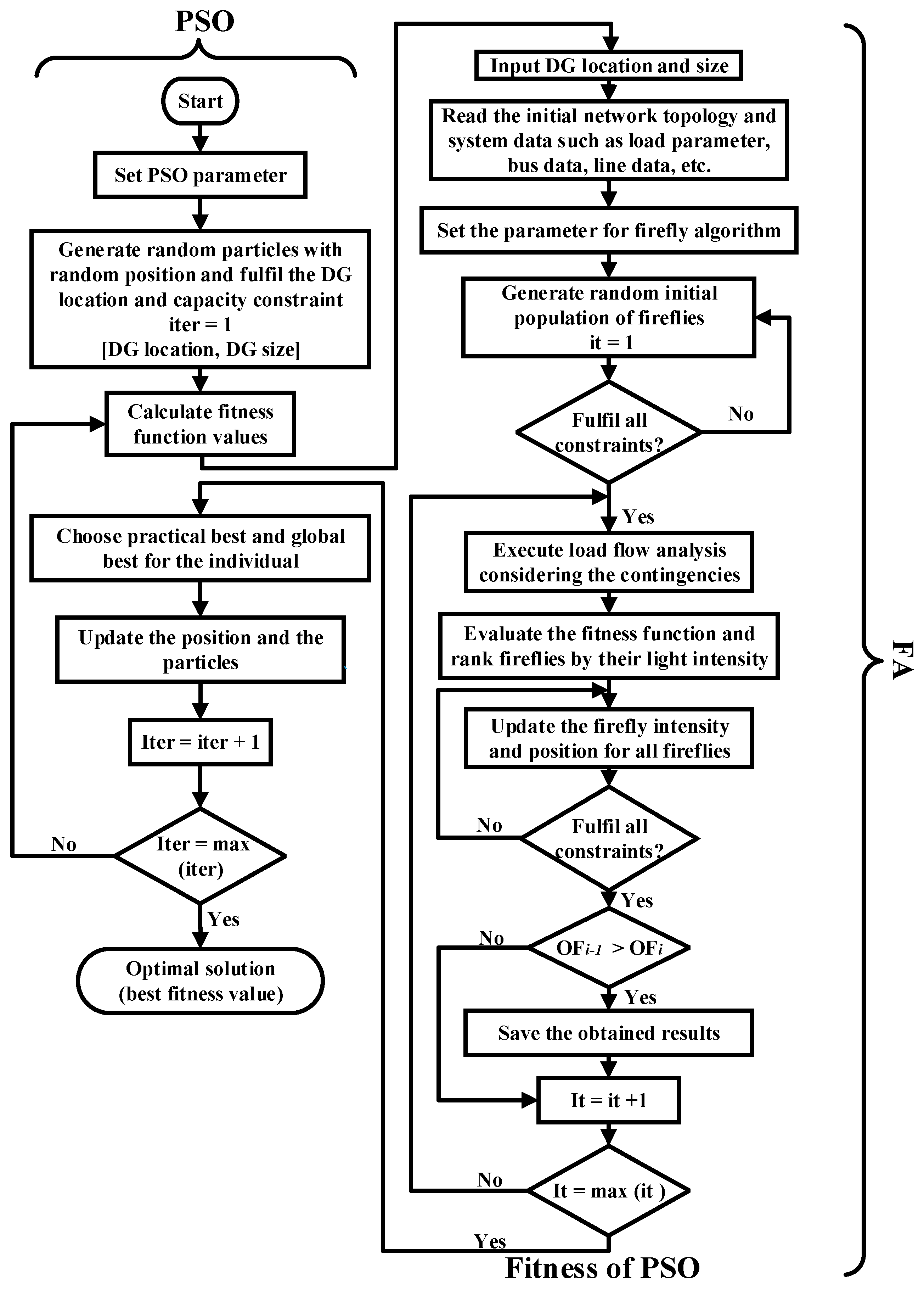
3. Proposed FA-PSO Technique for Distribution Expansion Planning

Distribution system expansion planning is a mixed-integer nonlinear and non-convex problem. In the past, most researchers considered mathematical optimization techniques such as MINLP or MILP for the expansion planning problem. However, these techniques are tend to get stuck in local optima. Therefore, researchers tend to reduce the search space by not considering the simultaneous optimization of N-1 contingencies for all branches, DG sizing and location, and multiple load profile to reduce the total investment and loss costs. On the other hand, metaheuristic techniques have a capability in handling mixed-integer and non-linear and complex optimization problems [6]. In this paper, a firefly algorithm and particle swarm optimization (FA-PSO) algorithm is proposed to optimize the DSEP problems because PSO has the potential to converge faster, while FA has the capability and the accuracy to get optimal solutions [27,28].

FA is a metaheuristic technique that is influenced by the attitude of fireflies and their scintillating patterns [29]. Depending on the flashing brightness, all fireflies will be attracted toward the one that has a higher brightness. Thus, the brightness of the flashing and the attraction are directly proportional while they are inversely proportional to the distance between the fireflies. If all the fireflies have similar radiant intensity, the fireflies will indiscriminately move from their particular position. Similarly, PSO is also inspired by nature, especially by the behaviors of birds and fish when they search for food. The essential concept of PSO is to update the velocity and position of the particles during the searching process [30]. The step-by-step FA-PSO algorithm for the distribution system expansion planning problem is described as follows:

Step 1: Initial input data

Enter the initial network data such as active and reactive power at each bus, resistance and reactance for each line, the present topological structure of the distribution network, number of DGs, contingencies on the branches, and the variable load profiles.

Step 2: Initialize the population for PSO

Like any metaheuristic techniques that depend on populations, the particles in PSO will generate random location and size of the DG based on the defined range for each of the variables; Equation (13) represents the PSO population.

$$P_{PSO}=\left[\begin{array}{c}\stackrel{PSO}{\overbrace{\begin{array}{cc}\begin{array}{c}DG location\\ DG lo{c}_1\\ \begin{array}{c}DG lo{c}_2\\ \begin{array}{c}⋮\\ DG lo{c}_n\end{array}\end{array}\end{array}& \begin{array}{c}\begin{array}{c}\begin{array}{c}DG Size\\ DG siz{e}_1\end{array}\\ DG siz{e}_2\\ ⋮\end{array}\\ DG siz{e}_n\end{array}\end{array}}}\end{array}\right]$$

(13)

where P_PSO refers to the PSO population which consists of the DG location and size and is presented by ($DG lo{c}_n$, $DG siz{e}_n$). After that, $DG lo{c}_n$ $\mathrm{and}$ $DG siz{e}_n$ will be as input for the FA.

Step 3: Initialize the population for FA

Similarly to the PSO technique, the population in the FA is indiscriminately initialized with the branch number that needs to be open. P_FA denotes the FA population, $X_{*,*}$ discrete number/value refers to the branches that should be open in the network, and $m$ refers to the number of branches and $n$ the number of populations.

$$P_{FA}=\left[\begin{array}{c}\stackrel{FA}{\overbrace{\begin{array}{c}\begin{array}{c}\begin{array}{c}Selected Branches\\ X_{11},X_{21},\cdots ,X_{m1}\\ \begin{array}{c}{X}_{12},X_{22},\cdots ,X_{m2}\\ ⋮\end{array}\end{array}\\ X_{1n},X_{2n},\cdots ,X_{mn}\end{array}\end{array}}}\end{array}\right]$$

(14)

Step 4: Evaluation of population

After executing the load flow analysis while considering the contingency for all branches, the optimization algorithms will optimize both DG size and location in addition to choosing the best configuration for the network by closing tie switches or opening them, decommissioning existing branches, constructing new switchgear/branches, and reinforcing switchgear/branches in order to minimize the total cost based on the objective function described in (1). Then, these populations are ranked based on their fitness. Rank ‘1’ is the preferable firefly in the current population.

U_i = f (x_i, ₁, x_i, ₂, x_i, ₃… x_i, _d)

(15)

where Ui is the cost of i^th population based on (1).

Step 5: Update firefly attractiveness and position

The fireflies update their attractiveness and movements according to the distance from the higher-ranked fireflies. Based on the distance from the higher-ranked fireflies, the fireflies will update their location and attractiveness.

$$s_{ij}=\Vert x_i-x_j\Vert =\sqrt{{{\displaystyle \sum }}_{u=1}^l{\left(x_{i,u}-x_{j,u}\right)}^2}$$

(16)

where $x_{i,u}$ and $x_{j,u}$ represent the $u^{th}$ component of the Cartesian coordinate $x_i$ and $x_j$ of fireflies i and j, respectively. The firefly attractiveness β can be specified according to the following equation:

$$\beta \left(s_{ij}\right)={\beta }_0{e}^{-\gamma s_{ij}{}^2}$$

(17)

where ${\beta }_0$ is the attractiveness when s = 0, $\gamma$ refers to the coefficient of light absorption and is normally set to 1 as a constant, α is the mutation coefficient, and $s_{ij}$ is the distance between any two fireflies. The movement of the fireflies, where the firefly i is attracted to firefly j, is determined by the following formula:

$$x_i=x_i+{\beta }_0{e}^{-\gamma s_{ij}{}^2}(x_j-x_i)+\alpha (rand-0.5)$$

(18)

The second term in Equation (18) is caused by the attraction, while the third term represents the randomized parameter and the random range being between 0 to 1. After updating and rounding to the nearest integer, check that all constraints are satisfied.

Step 6: Update PSO position and velocity

When the number of iterations in the FA reaches the maximum, the best network configuration is selected. Selected configuration return to PSO and the best fitness value from the FA will be the cost for PSO population. Therefore, PSO will update the location and the size of the DG, and then it will enter again as input to FA. Accordingly, FA will choose new network reconfiguration based on the new DG size and location to attain the minimum total cost. Hence, PSO will choose the particle best and global best then both velocity and position, or each particle will be updated and rounded to the nearest integer according to Equations (19)–(21):

$$z_a^{b+1} = z_a^{b }+s_a^{b+1}$$

(19)

$$W=w_h- (\frac{w_h-w_l}{ite{r}_h})·iter$$

(20)

$$s_a^{b+1} =W·s_a^b+c_1{r}_1·(E_{best,a}-z_a^{b }) +c_2·(G_{best,a}-z_a^{b })$$

(21)

where $z_a^{b }$ and $z_a^{b+1}$ indicate the current position for the particle a at iteration b whereas $s_a^b$ and $s_a^{b+1}$ refer to the current velocity of particle a at iteration b and b+1, respectively. Finally,$w_h$ and $w_m$ represent the highest and lowest weight of the inertia, respectively. The acceleration constants are represented by $c_1$ and $c_2$ while the global best and the particle searching experience are denoted by $G_{best}$ and $E_{best}$, respectively; they were chosen based on hit and trial, and $E_{best}$ represents the best solution coordinates that this specific person has so far obtained while $G_{best}$ refers to the overall best solution obtained by PSO.

Step 7: Terminus conditions

The process will be repeated from “Step 4 to 6” until the cost difference between all populations’ fitness values is less than the specified deviation or the maximum number of iterations is reached. The optimal solution provides the best DG location, size, and optimal network configuration, and the evaluation of the optimal solution provides the minimum investment and loss cost for the expansion planning. The FA-PSO attains a single optimal expansion planning solution for all branches under N-1 contingencies and variable load profile. The flowchart in Figure 1 demonstrates how FA-PSO algorithms were employed to solve the DSEP problem. The parameters applied in the proposed technique were chosen based on the empirical analysis in terms of finding an optimal solution with reasonable computational time; the number of populations and the other parameters that were used in this work were feasible to achieve our aims, and it is demonstrated in

Table 1. FA-PSO parameters.

Parameters	p	γ	∅	β	α	w	$c_1$	$c_2$
Values	20	1	0.8	2	0.2	1	1.5	2

.

4. Results and Dissection

In this work, IEEE 33- and 69-bus distribution systems were utilized to validate the performance of the proposed approach. The network parameters used in [12] were assumed for this paper, and they are as follows: cost of branch construction/reinforcement (44,600 GBP/km), cost of constructing/upgrading switchgear (5000 GBP/unit), cost of branch decommissioning (1000 GBP/km), and terminal cost (5000 GBP/branch). In this work, PV is assumed for the distributed generator with an installation cost of 548 GBP/kW capacity, as specified in [19]. The cost of power losses is taken as 0.054 GBP/kWh [31]. In addition, the maximum allowable capacity of the DG planned to be installed ($CD{G}_i$) is limited to 2000 kW and 2500 kW for the 33- and 69-bus systems, respectively, taking into consideration the overall load demand of the system. Three case studies are presented in this section to highlight the contribution of the paper. The case studies are as the following:

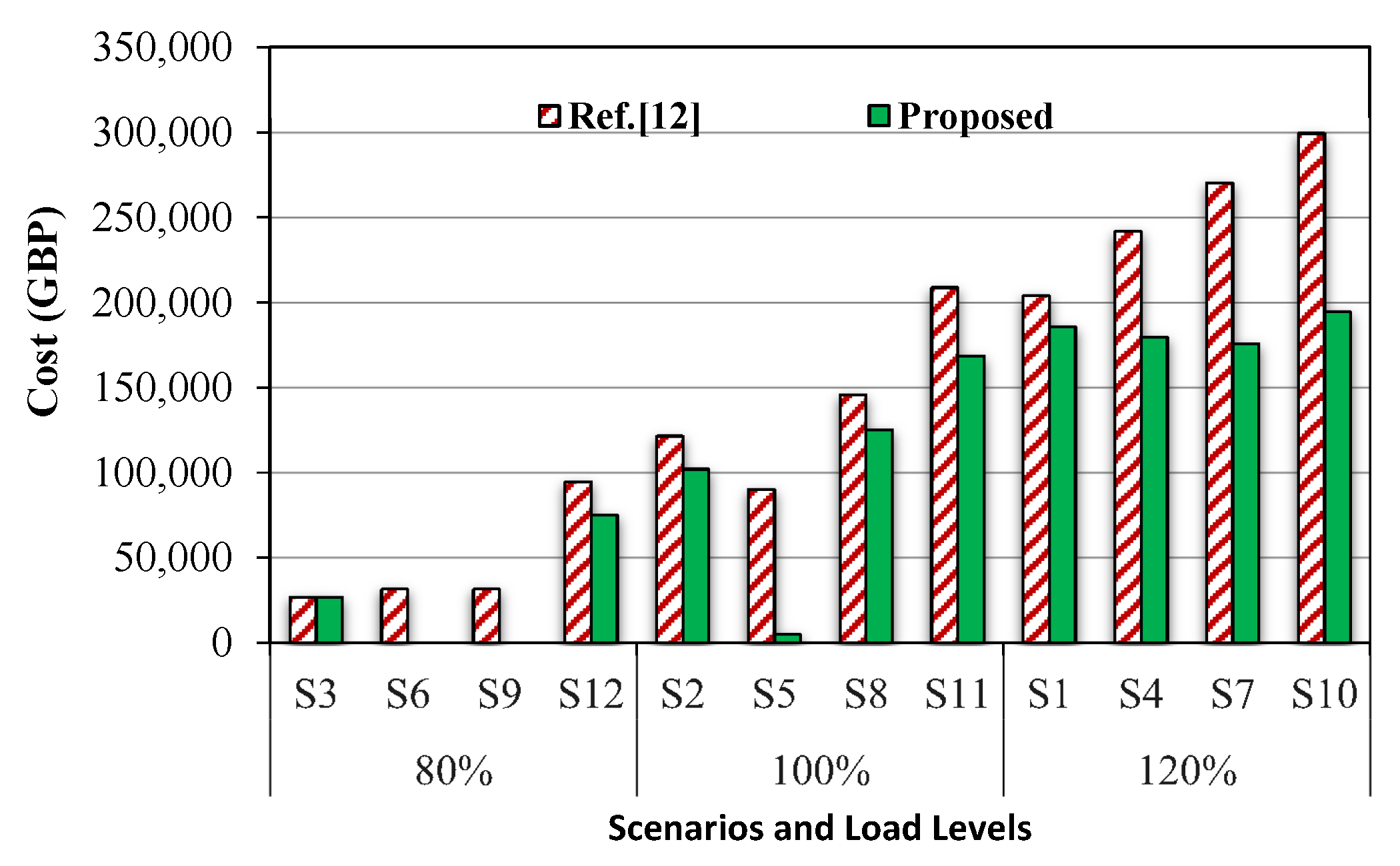
• Case 1: Load profiles of the system are represented using three load levels for two consecutive 5-year planning periods. In addition to the normal operation of the network, three ‘crucial’ branches are independently put on outage to highlight the efficacy of the FA-PSO algorithm in comparison to the method proposed in [12].
• Case 2: Case 1 above is further expanded by considering variable load profiles by including 24 load levels. All branches are independently put on an outage. Furthermore, the impact of DGs is demonstrated through two scenarios. The DG is neglected in scenario A, whereas DG size and location are simultaneously optimized in scenario B. One expansion planning solution is determined at the end of each scenario.
• Case 3: Continuing from Case 2, the same load profile is used but in ordinary operation without any contingencies. One optimal expansion planning solution is obtained at the end of this case with optimal DG size and location.

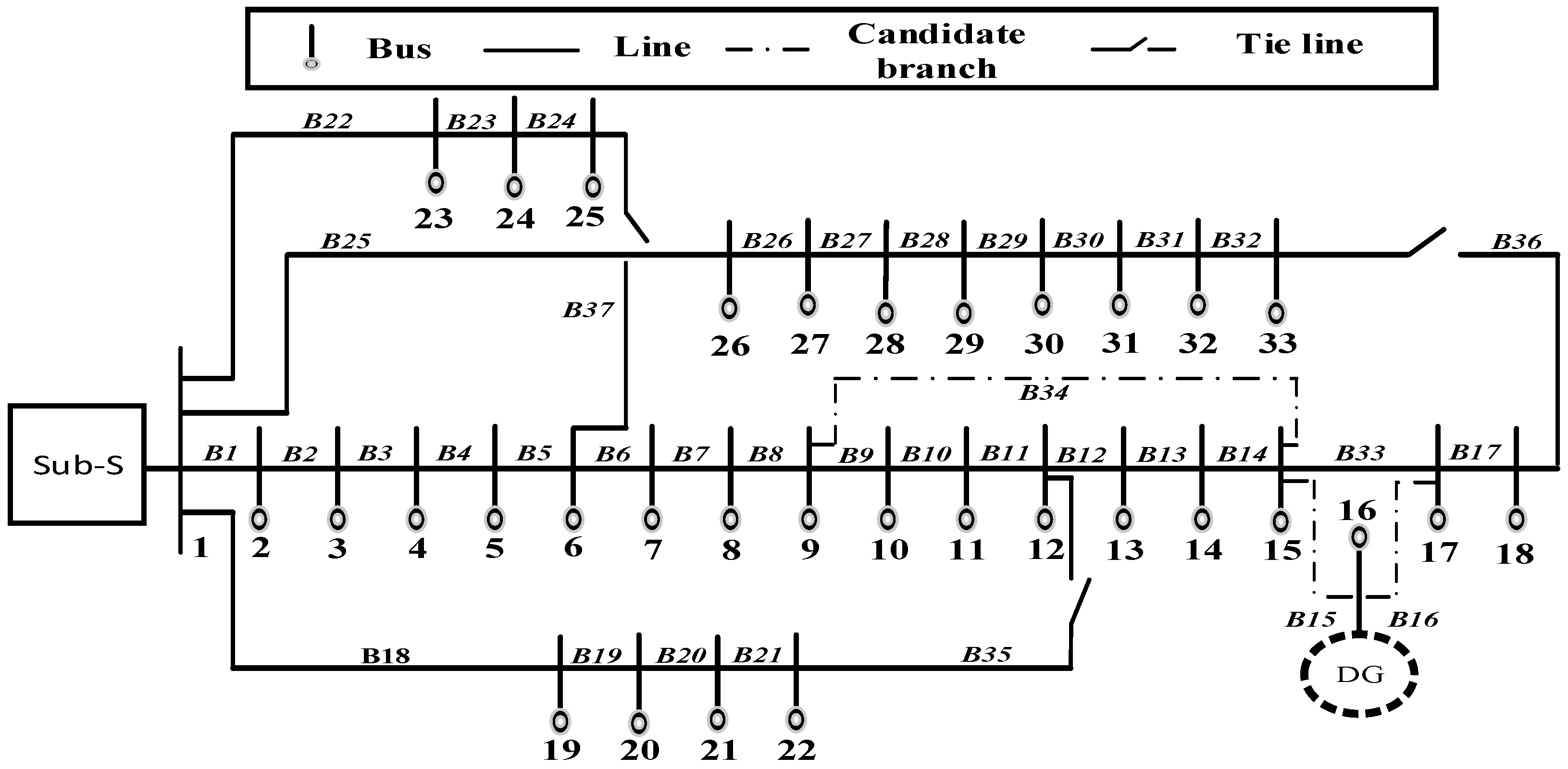
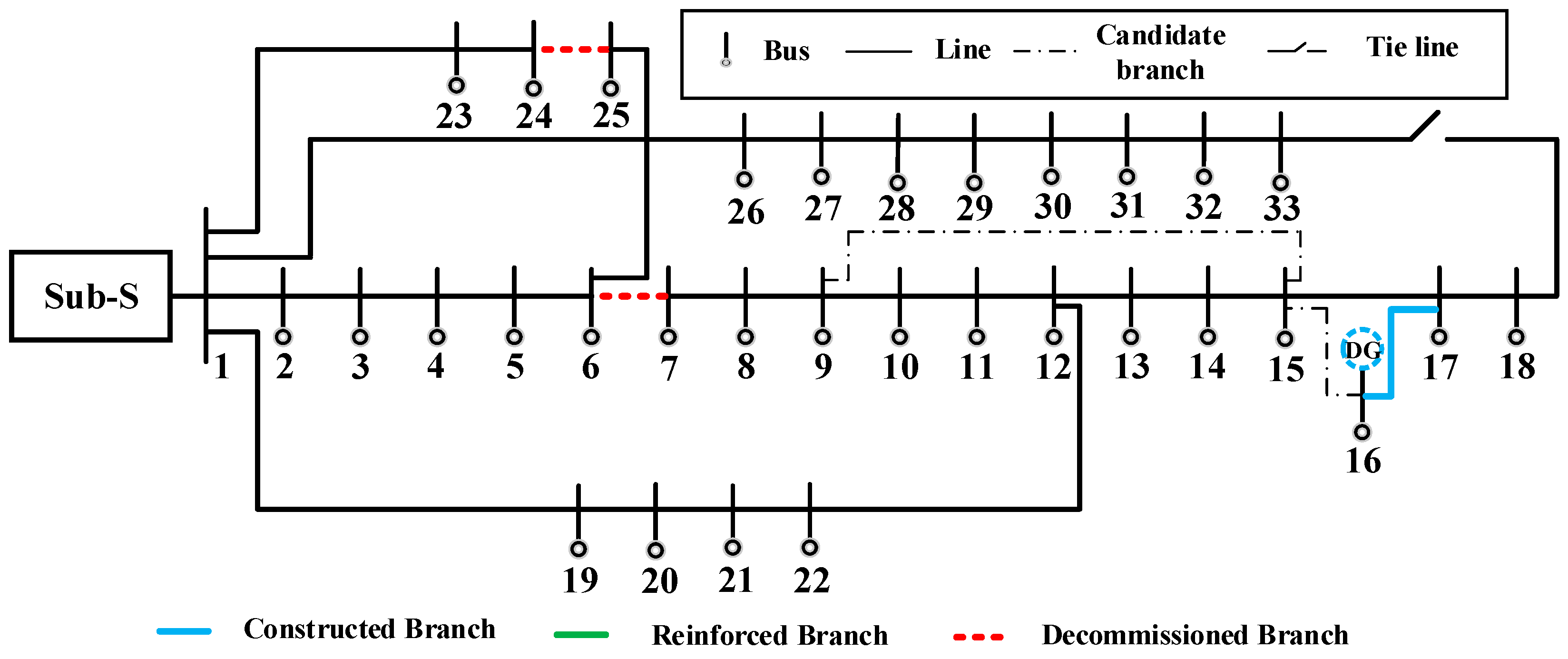
4.1. Test System 1: IEEE 33-Bus

In this paper, an IEEE 33-bus distribution network as shown in Figure 2 is used to validate the proposed method. The system consists of sectionalizing and tie switches as well as potential routes to construct new branches that might possibly be used to reconfigure the network. A new connection of a DG is also proposed to the network to enhance the system performance in addition to minimizing the total system power losses. In the default condition, DG is assumed to be located at bus 16 and can be connected to the network through either branch B15 or B16, and the capacity of the DG will be determined by the system operator. The candidate branches to connect the DG or to construct a new branch are represented by a dashed line in Figure 2.

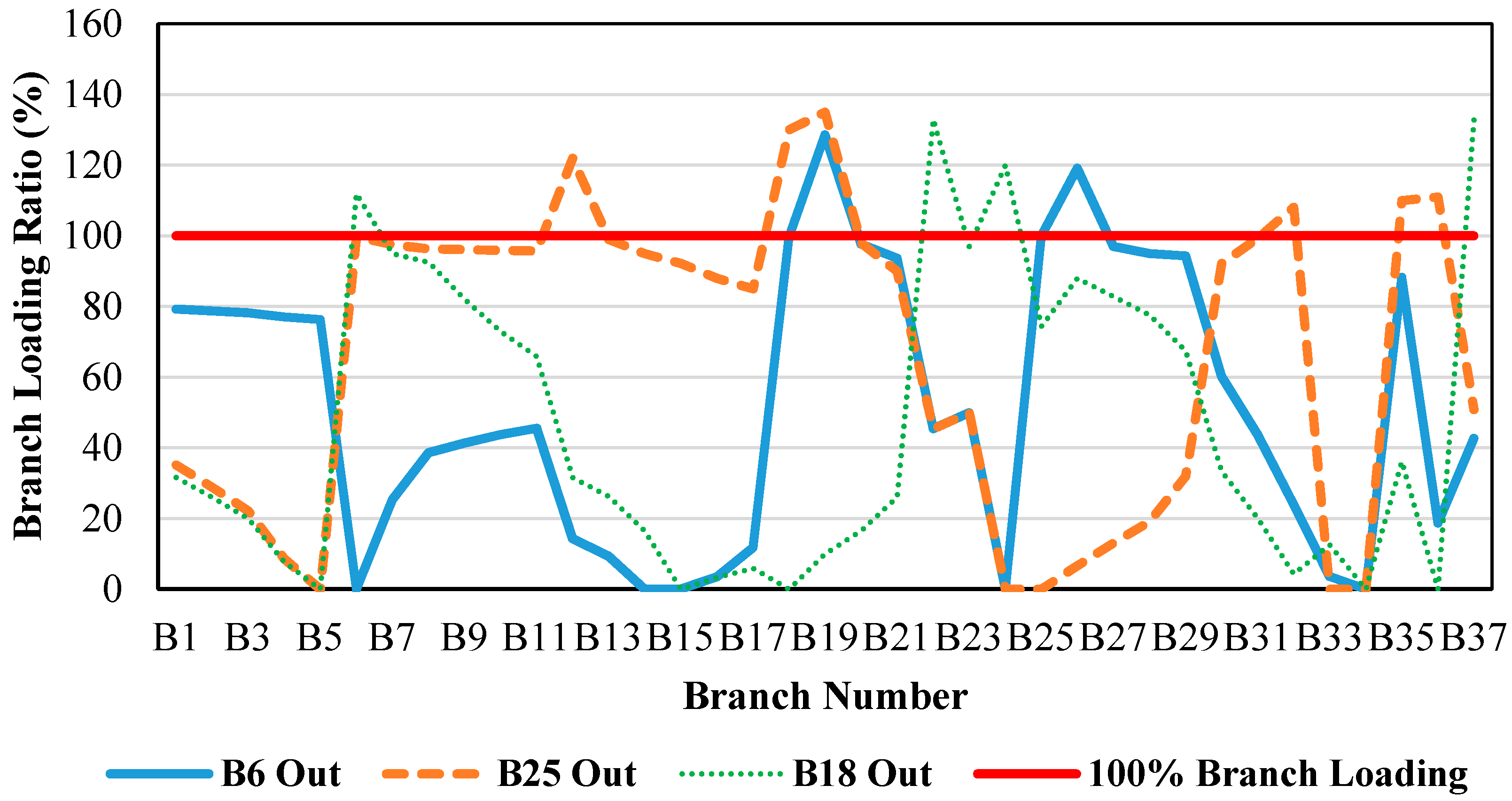
4.1.1. Case 1: Three Critical Branches’ Outage

As outlined earlier, Case 1 considers an independent outage of three ‘crucial’ branches considering three load profiles in a year. To validate the performance of the proposed method, Ref. [12] is taken as the main comparison considering the investment cost only (OF₁). Under this case study, 12 scenarios are considered where S1, S2, and S3 indicate scenarios in the first planning period correlated to 80%, 100%, and 120% from the peak demand loads specified in [12], while S4, S5, and S6 indicate scenarios in planning period 2 resulting from scenario 1 in planning period 1. The remaining scenarios are set up following the same format. A 25% load growth is assumed in planning period 2 from planning period 1. The same branches as in [12] are assumed as the ‘crucial branches’—branches connecting buses 1–2, 9–10, and 12–13 due to their significant impact on the system.

Table 2. Comparison of the total investment costs for 33-bus system.

First Planning Period
Scenario	S1			S2			S3
Load level	120%			100%			80%
Costs (GBP) [12]	204,128			121,782			26,854
Proposed (GBP)	186,034			102,252			26,854
Improvement	8.86%			16.03%			0%
Second Planning Period
Scenario	S4	S5	S6	S7	S8	S9	S10	S11	S12
Load level	120%	100%	80%	120%	100%	80%	120%	100%	80%
Costs (GBP) [12]	242,052	90,468	31,760	270,640	145,960	31,760	299,690	209,128	94,928
Proposed (GBP)	179,806	5000	0	176,108	125,542	0	194,696	168,730	75,398
Improvement	25.71%	94.4%	100%	34.92%	13.98%	100%	35.03%	19.31%	20.5%

summarizes the capital investments needed to optimally expand the network along with the results previously obtained in [12].

Table 3. Assets installation and upgrading for 33-bus system.

Assets Construction and Reinforcement
Scenario	Proposed Method
S1	Branch: $\overline{\mathrm{B}16}$, $\overline{\mathrm{B}34}$, B19, B22, B23, B24 Switchgear: $\overline{\mathrm{B}6}$, $\overline{\mathrm{B}7}$, $\overline{\mathrm{B}24}$, B22 Branch Decommissioning: B31
S4	Branch: B22, B23, B24, B26, B27, B37 Switchgear: B22, B24, B37 Branch Decommissioning: B7

elaborated the assets installation/upgrading for S1 and S4 determined using the proposed method. Figure 3 plots the investment costs for each scenario, and it can be seen that results obtained using FA-PSO are consistently lower as compared to the method proposed in [12]. The proposed FA-PSO has the capability to find a global optimal solution for a complex DSEP problem while discrete mathematical modeling used in [12] is highly dependent on the initial conditions of the problem to progress to the intended solution and has the potential to get stuck in the local optima. In conclusion, the improvement in the total costs in % is shown below each scenario.

In Table 3, the blue color and upper line refers to the constructed branch/switchgear whereas the green color refers to reinforced branches; finally, the red color refers to decommissioned branches. In S1, branches B16 and B34 will be constructed, and four branches will require reinforcement. In the case of switchgear, three switchgears were installed, and one was upgraded. Finally, branch B31 got decommissioned. The load in the second planning period will increase by 25%, and added to the original load, in S4, six branches are upgraded—three of them were reinforced previously in S1, three switchgears on branches B22, B24, and B37 were reinforced, and branch B7 got decommissioned—while there are no constructed branches because they were already installed in the first planning period. Similar trends were applied to the other scenarios. The zero cost in S6 and S9 denoted that the system is operated normally without any violation of the branches’ current limits, and the installation/reinforcement of any network assets is not required. It is evident that the proposed method obtains a solution with lower costs as compared to Ref. [12]. Furthermore, it should also be noted that the proposed method considers all branches to be on outage and still obtains one optimal solution for better network planning to avoid the hazardous faults that may occur in other branches. This is a more pragmatic approach which Ref. [12] did not adopt.

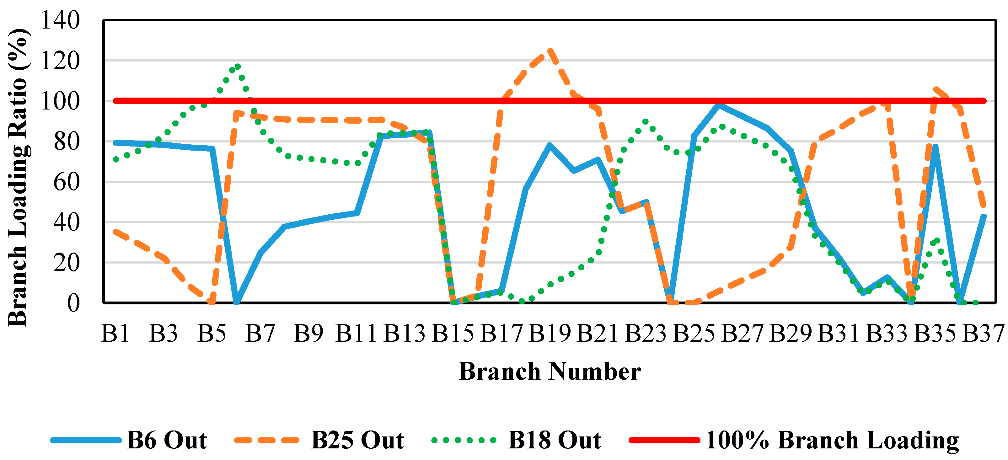
4.1.2. Case 2: All Branches’ Outage

In this case, all the branches are considered on outages one by one. This case consists of two scenarios: in the first one, the DG will not be considered while taking the contingency for all branches, whilst in the second one, the DG size and location will be optimized while considering the contingency for all branches. One optimal solution will be obtained at the end of each scenario.

Scenario A: All Branches N-1 without DG

All branches of the IEEE 33-bus system are independently put on outage for 24 different load profiles varying from 70% to 100% [32] rather than considering only annual peak demand. Only a single-stage, 5-year planning period is assumed in this case without considering DG integration. The total investment and loss cost determined using the proposed FA-PSO method was GBP 679,451, where the investment cost (OF₁) was GBP 465,580 and accounted for 68.52% of the total expansion planning cost. On the other hand, the cost of the power losses amounted to GBP 213,871 (OF₃) for the five-year planning period (31.48% of the total cost). The maximum power losses occurred when branch B25 was on outage while the load was 100%; meanwhile, the minimum losses happened when branch B10 was put on outage when the load was at 70%.

Table 4. Total investment cost for 33-bus system expansion planning without DG.

Investment Cost When All Branches Outage without DG for 33-Bus System (OF1)
	Constructed	Reinforcement	Switchgear	Deco.	Total
Branches	B16, B34	B1, B6, B12, B13 B18, B19, B22 B24, B26, B32 B35 B36, B37	B1, B5, B6, B10, B14 B17, B18, B22, B24 B33, B35, B36, B37	-
Cost (GBP)	55,492	345,088	65,000	0	465,580

lists the branches required to be upgraded; 13 branches need to be reinforced with a total cost of GBP 345,088, representing around 74.12% of the total investment cost, whereas the cost of the constructed branches was the lowest, accounting for 11.9% of the total investment cost. In addition, thirteen switchgears were required to be installed/upgraded in the network with a total expenditure of GBP 65,000. Figure 4 illustrates the ratio of the current flowing in the lines to the respective line capacity for the case of branches B6, B18, and B25 on outage. These lines were considered because of their effect on the entire system during contingency in terms of exceeding the thermal capacity and the installation of new switchgears on other branches. It can be seen from Figure 4 that the currents that exceed the thermal capacity of the branches require reinforcement. For instance, when branch B25 is on outage, six branches need reinforcements, and three switchgears are required to be installed on branches B5, B33, and B24. Similarly, when branch B18 was on outage, four branches violated the thermal capacity, and thus branches B6, B22, B24, and B37 need to be upgraded with higher thermal capacity and one switchgear needs to be constructed in branch B5. Finally, when branch B6 was on outage, two branches B19 and B26 needed to be uprated while two switchgears needed to be constructed in branches B14 and B24.

It can be concluded from the results that if DG was not considered during system planning, it would lead to more violation in the thermal capacity of the branches. This in turn necessitates additional investments to be spent to construct and upgrade equipment in the network. Moreover, power losses in the system would remain high, and there is no flexibility to feed the out-of-supply loads in the network during contingencies. Despite reducing the DG installation costs by not having to implement the DG into the network, system performance and efficiency were negatively affected.

Scenario B: All Branches N-1 with Optimizing DG Size and Location Simultaneously

In the second scenario of this case study, the location and the size of the DG are determined considering N-1 contingency for all branches in the network. The same loads are considered as in scenario A for the static planning period. Based on the proposed method, the optimal location and size for the DG to achieve minimum investment and loss costs was on bus 15 with 1727 kW as the maximum DG output.

Table 5. Total investment cost for 33-bus system expansion planning with DG sizing and location.

Investment Cost When All Branches Outage with DG for 33-Bus System (OF1)
	Constructed	Reinforcement	Switchgear	Deco.	Total
Branches	B16, B34	B1, B6, B18, B19 B23, B35	B1, B5, B6, B8 B10, B18, B24, B31 B35	-
Cost (GBP)	55,492	168,706	45,000	0	269,198

shows the total investment cost when outage on all branches was considered with one DG output.

One solution is obtained with the total investment and loss cost of GBP 1,398,167; the net present value of the investment cost to construct/upgrade branches and switchgears for a five-year planning period (OF₁) is GBP 269,198, accounting for 19.2% of the total investment and operational cost, in addition to the DG installation cost (OF₂) of GBP 946,396 and power loss cost (OF₃) of GBP 182,573 which account for around 67.7% and 13.1% of the total costs, respectively. The highest and lowest losses occurred/were observed when branches B25 and B11 were on outage, respectively. It can be observed from Table 5 that two branches need to be constructed with a total cost of GBP 55,492, while most of the expenses occurred in the reinforcement part, and six branches need to be upgraded with a ratio of 62.6% of the total investment cost. Finally, in the switchgear section, nine switchgears were required to be constructed/reinforced with an expenditure of GBP 45,000 which represents 16.7% of the total investment cost. In the same manner as the previous case, Figure 5 shows the ratio of the branch current for some contingency cases, indicating branches needed to be reinforced. The number of violations in the current limits (Equations (8) and (9)) was reduced after connecting the DG unit at the optimal location with a suitable size in the network.

When branch B25 is on outage, three branches need to be reinforced, in addition to the construction of two switchgears on branches B5 and B24. On the other hand, when branch B18 was on outage, only branch B6 needed an upgrade and no need to construct nor reinforce any switchgears. Meanwhile, in the case of branch B6 outage, no branch was required to be reinforced, and only one switchgear needed to be constructed in branch B24.

The solution obtained ensures the network meets the growing load demands with minimum investment and loss costs, and in the case of contingency, DSO has the capability to restore the network in a timely manner. In addition, integrating DG during network planning will help to reduce the total investment and loss costs. However, optimal capacity and location would ensure a greater benefit. Furthermore, DG integration into the network will reduce the cost of network and asset reinforcement. Comparing to scenario A, it was observed that the total investment costs for scenario B decreased by about 42.18% and the power losses by 14.63% after connecting the optimal DG capacity at the optimal location. Hence, it can be concluded that a significant impact of DGs can be harvested when it is properly considered in the early planning of the distribution system.

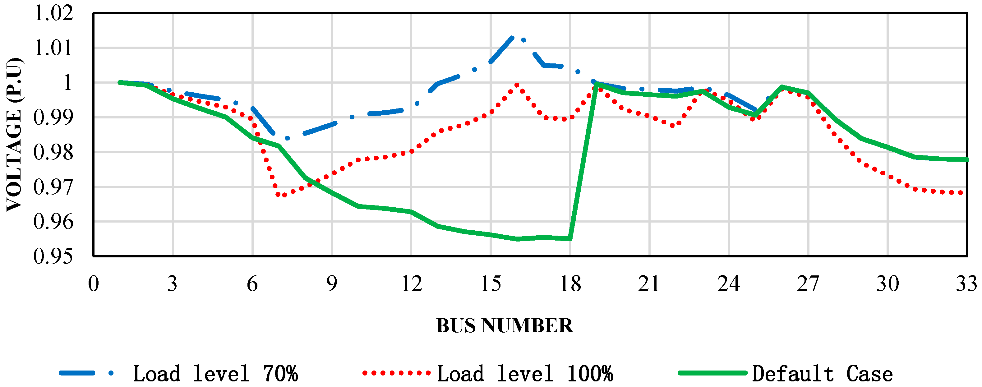
4.1.3. Case 3: Normal Operation with Optimizing DG Size and Location

In this case study, the expansion planning for the 33-bus system in normal operation is explained. One optimal solution for the different 24 loads in optimal operation is obtained using FA-PSO for optimization. The results show that the optimal DG size and location for all different loads were 1280.84 kW at bus 16. The total cost was GBP 877,836.5 divided among three terms. The first one is the total investment cost (OF₁) for the one solution, and it was GBP 27,804; the DG installation cost (OF₂) was GBP 701,900; and finally, the total power losses (OF₃) were GBP 148,132.5. Only one branch is constructed (branch B16) to connect the DG, two branches were decommissioned (B6 and B24), and there is no need to reinforce any branch nor construct switchgear. Figure 6 illustrates the new configuration for the system, while

Table 6. Total investment cost in normal case with different load level.

Normal Case (without Contingencies) for 33-Bus System
	Constructed	Reinforcement	Switchgear	Decommissioned	Total
Branches	B16	-	-	B6, B24
Cost (GBP)	26,854	0	0	950	27,804

shows the branches that need to be constructed and decommissioned in this case. Figure 7 plots the voltage profile in the normal case when the DG is not connected and after the reconfiguration of the existing system topology when the load levels are at a maximum and minimum value. It can clearly be noted that the voltage profile improved along with the materialization of the planning solution found in this case, in addition to DG integration. Furthermore, all the network constraints were satisfied. The highest voltage was observed when the load level was 70%, where it reached the peak with a value of 1.0145 p.u. The lowest value was observed in the default case where it dramatically decreased until reaching the bottom with a value of 0.9549 p.u. On the other hand, in a 100% load level, the voltage at each bus fluctuated and ended up with maximum and minimum values of 1 and 0.9670 p.u, respectively. Moreover, a spike was observed on bus 16 because a DG is connected to this bus.

In this case, the total investment cost for the planning of the distribution networks in normal operation is relatively small compared to the other two cases, but in the case of contingency, violation of thermal limits for the feeders might happen, resulting in some buses being disconnected from the supply. For instance, if a fault happens in branch B23, bus 24 will be out of supply and the current in some branches will exceed the thermal capacity. This indicates the importance of considering N-1 contingency during the planning exercise to predict and plan loads restoration, in addition to the normal planning to meet the load growth and maintain system sustainability during contingencies.

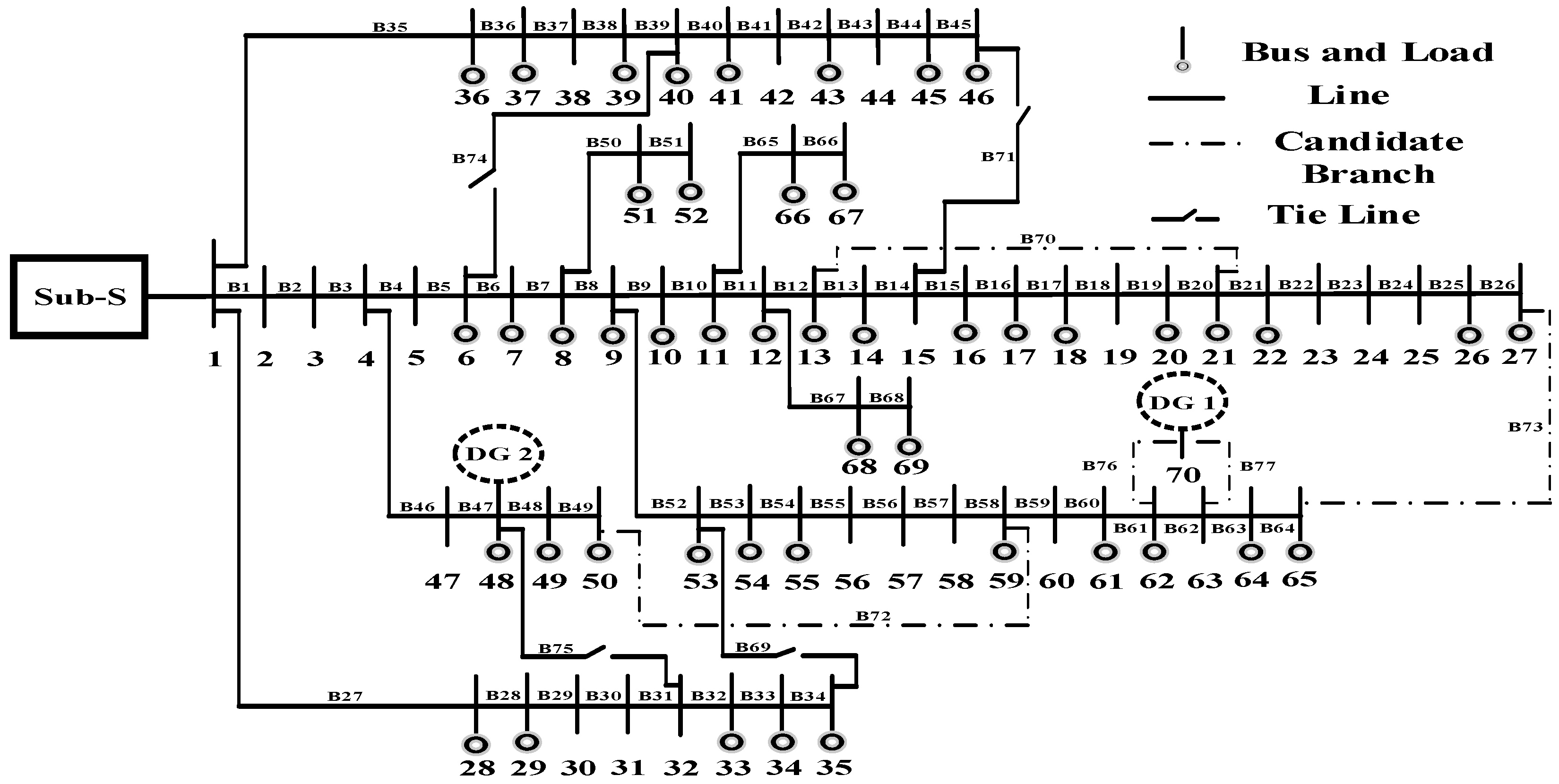
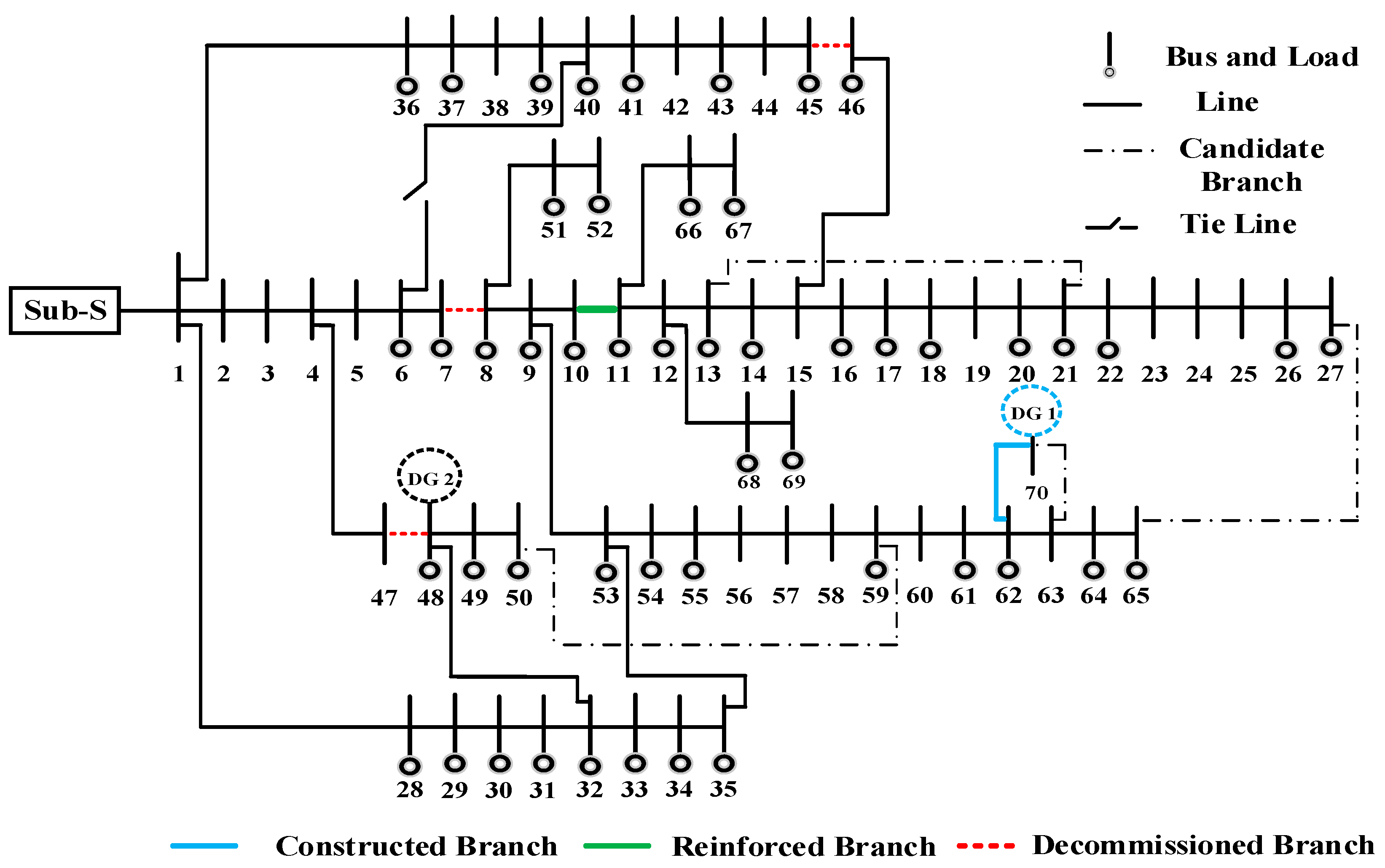
4.2. Test System 2: IEEE 69-Bus

Another test, a 69-bus system [33], was examined to validate the proposed approach. As shown in Figure 8, the system consists of three main 12.66 kV feeders in addition to five candidates’ places B70, B72, B73, B76, and B77 to construct new branches (dashed lines). From these, two connected branches B76 and B77 can be used to implement the DG 1 (which is located at bus 70) in the default case to the network whereas DG 2 will be on bus 48.

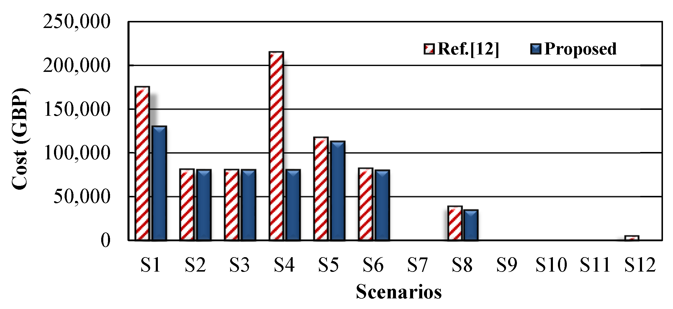
4.2.1. Case 1: Three Critical Branches’ Outage

Under this case study, 12 scenarios are considered where S1, S2, S3, and S4 indicate scenarios in the first planning period correlating to 80% and 100% from the peak demand loads in addition to 100% and 150% from the DGs’ output specified in [12], while S5 and S6 indicate scenarios in planning period 2. S5 and S6 are based on the results of scenario 1 in planning period 1, as they investigate the feasibility of connecting the second DG (DG 2). For S5, the DG 2 loading is 100%, and for S6, the DG 2 loading is 150%. Furthermore, the load level in S5 and S6 is increased by 25% from the load level of S1. The remaining scenarios are set up following the same format, i.e., S7 and S8 from S2, S9 and S10 from S3, and S11 and S12 from S4. The first case study considers the contingency of specific three branches B1, B6, and B53. The first DG (DG 1 at node 70) will connect to the network in the first planning period while the second DG (DG 2 at bus 48) will integrate into the system in the following planning period for this case study only.

Table 7. Comparison of the total investment costs for 69-bus systems.

First Planning Period
Scenario	S1		S2		S3		S4
Load level (%)	100%		100%		80%		80%
DG 1 (%)	100%		150%		100%		150%
Costs (GBP) [12]	175,452		81,406		80,900		215,208
Proposed (GBP)	130,444		80,656		80,656		80,656
Improvement	25.6%		0.92%		0.3%		62.5%
Second Planning Period
Scenario	S5	S6	S7	S8	S9	S10	S11	S12
DG 2 (%)	100%	150%	100%	150%	100%	150%	100	150%
Costs (GBP) [12]	117,674	82,440	0	38,990	0	0	0	5000
Proposed (GBP)	113,008	80,004	0	34,770	0	0	0	0
Improvement	3.96%	2.95%	0%	10.8%	0%	0%	0%	100%

demonstrates a comparison between the proposed method and the work in [12]. The results show that the cost for some scenarios is nearly the same, especially in S7, S9, S10, and S11 where the total cost was zero. The best minimization in cost occurred in S12, where the total cost was reduced by around 100%, followed by S4 with a reduction in total investment cost by 62.5%, and finally, in S1, it was reduced by 25.6%. In the other scenarios, the costs were slightly decreased; for instance, in S8, S5, S6, S2, and S3, the costs diminished by 10.8%, 3.9%, 2.9%, 0.92%, and 0.3%, respectively.

Figure 9 presents the results in bar chart form to compare the cost for each scenario. Four scenarios in the second planning period did not require any type of construction/reinforcement for any branch or switchgear with GBP 0 cost. The highest cost in the proposed method occurred in S1 and S5 with the cost of GBP 130,444 and GBP 113,008, respectively. Similarly, with the previous test system,

Table 8. Asset installation and upgrading for 69-bus system.

Asset Construction and Reinforcement
Scenario	Proposed Method
S1	Branch: $\overline{\mathrm{B}72}$, $\overline{\mathrm{B}76}$, B29
	Switchgear: $\overline{\mathrm{B}2}$, $\overline{\mathrm{B}6}$, $\overline{\mathrm{B}56}$, $\overline{\mathrm{B}58}$
S5	Branch: $\overline{\mathrm{B}73}$, B48, B49
	Branch Decommissioning: B45

demonstrates the assets installation/upgrading for S1 and S5 determined by utilizing the proposed method for both planning periods. In the first planning period, two branches were constructed and only one branch was required to be upgraded whereas four switchgears were installed. For the second planning period, only branch B73 was constructed, two branches were reinforced, and branch B45 was decommissioned.

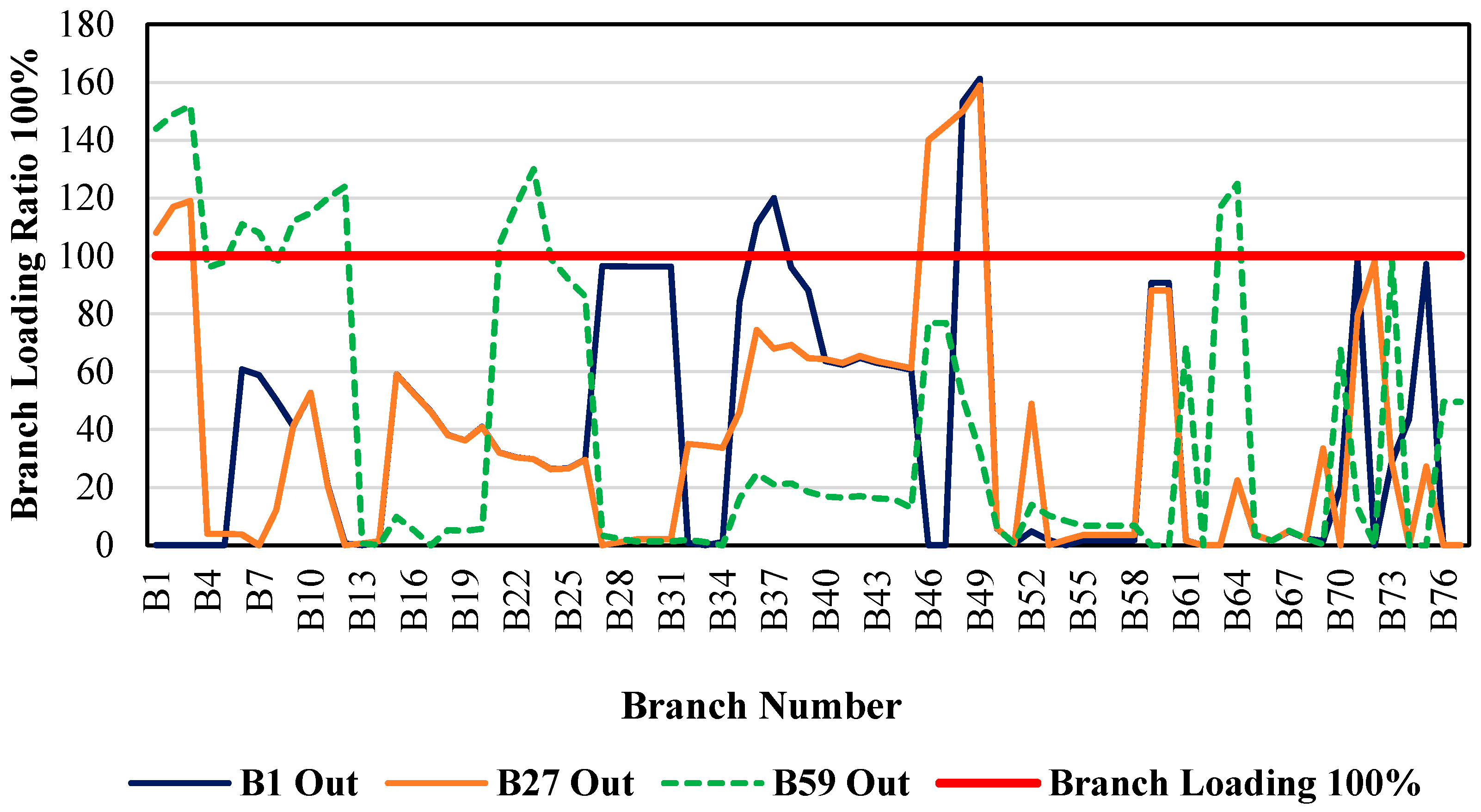
4.2.2. Case 2: All Branches’ Outage

Two scenarios were considered in this case similar to the scenarios in the 33-bus system. In the first scenario, outages on all branches are considered without a DG, while in the second scenario, outages on all branches are considered with optimizing DG size and location. One optimal solution is obtained at the end of each scenario.

Scenario A: All Branches N-1 without DG

All branches of the test system are independently put on outage considering the 24 load levels used in the 33-bus system. Only a single-stage, 5-year planning period is assumed in this case without considering DG integration. The total investment and power loss cost determined using the proposed FA-PSO method was GBP 1,261,713.85, where the investment cost (OF₁) was GBP 952,520, accounting for 75.5% of the total expansion planning cost. On the other hand, the cost of the power losses (OF₃) amounted to GBP 309,193.85 for the five-year planning period (24.5% of the total cost). The maximum losses occurred when branch B60 was on outage while the load was 100%. Meanwhile, the minimum losses happened when branch B29 was put on outage when the load was at 70%.

Table 9. Total investment cost for the 69-bus system expansion planning without DG.

Investment Cost When All Branches Outage without DG for 69-Bus System (OF1)
	Constructed	Reinforcement	Switchgear	Deco.	Total
Branches	B70, B72 B73, B76 B77	B1, B2, B3, B6, B7 B9, B10, B11 B12, B21, B22, B23 B36, B37, B46, B47 B48, B49, B55, B56 B63, B64	B1, B4, B7, B12, B13 B14, B17, B20, B33 B34, B46, B47, B53 B54, B62, B63	-
Cost (GBP)	181,100	691,420	80,000	0	952,520

lists the branches required to be upgraded; 22 branches need to be reinforced with a total cost of GBP 691,420, representing around 75.58% of the total investment cost, whereas the cost of the constructed branches was the lowest, accounting for 19% of the total cost. In addition, sixteen switchgears were required to be installed/reinforced in the network with a total expenditure of GBP 80,000. Figure 10 illustrates the ratio of the current flowing in the branches to the respective branch capacity for the case of branches B1, B27, and B59 which were on outage. These branches were chosen based on their impact on the whole network during the contingency in terms of the current violation and construction of new switchgear. It can be seen from Figure 10 that the currents that exceed the thermal capacity of the branches require reinforcement. For instance, when branch B1 was on outage, four branches needed reinforcement and five switchgears were required to be installed on branches B4, B13, B33, B54, and B63. Similarly, when branch B27 was on outage, seven branches violated the thermal capacity, and thus branches B1, B2, B3, B46, B47, B48, and B49 needed to be upgraded with higher thermal capacity; four switchgears needed to be constructed as well. Finally, when branch B59 was on outage, the highest violation in branches’ thermal capacity occurred with fourteen branches needing to be uprated while four switchgears required to be constructed in branches B14, B17, B34, and B62.

From the results above, it can be deduced that neglecting DGs through the planning for the distribution system results in an increase in the number of branches violating their thermal capacity. This leads to additional costs that are incurred to upgrade the branches and to construct new equipment in the network. Furthermore, the power losses remain high in addition to decreases in load serviceability during the contingences. In spite of minimizing the total cost by excluding the DG installation costs, the performance and the quality of the system were influenced negatively.

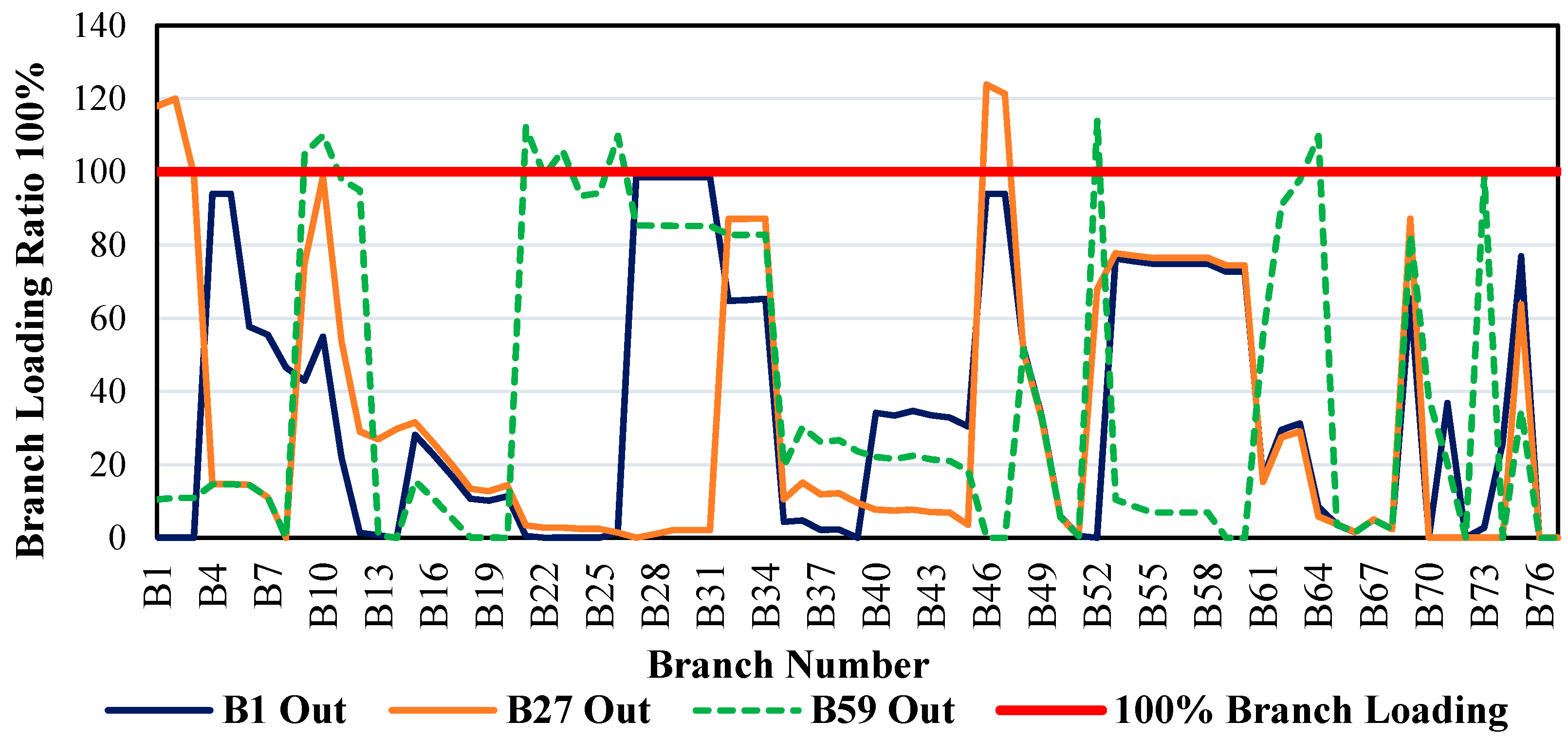
Scenario B: All Branches’ Outage with Optimizing DG Size and Location Simultaneously

In the second scenario of this case study, the system is similar to the above-discussed scenario, only DG size and location are optimized while considering all branches’ outage. One DG output is considered for all contingencies to optimize the optimal expansion planning investment and loss cost. The best location and size for the DG to attain minimum investment and loss cost was on bus 61 with 2345 kW as the maximum DG output.

Table 10. Total investment cost for 69-bus system expansion with DG sizing and location.

Investment Cost When All Branches Outage with DG for 69-Bus System (OF1)
	Constructed	Reinforcement	Switchgear	Deco.	Total
Branches	B70, B72 B73, B76 B77	B1, B2, B9, B10, B21 B23, B26, B46, B47, B52, B64	B1, B4, B6, B8 B14, B20, B25 B39, B45, B46, B52, B53, B62	-
Cost (GBP)	181,100	406,002	65,000	0	652,102

shows the total investment cost when outage on all branches with one DG output is considered. One solution is obtained with a total investment and loss cost of GBP 2,209,160; the net present value of the investment cost (OF₁) to construct/upgrade branches and switchgears for a five-year planning period is GBP 652,102 which accounted for 29.5% of the total investment and loss costs, in addition to the DG installation cost (OF₂) of GBP 1,285,060 and power loss cost (OF₃) of GBP 271,998 which is around 58.17% and 12.3% of the total costs, respectively.

It can be observed from Table 10 that five branches need to be constructed with a total cost of GBP 181,100; while most of the expenses occurred in the reinforcement part, eleven branches need to be upgraded with a ratio of 62.2% of the total investment. Finally, in the switchgear section, thirteen switchgears are required to be constructed/reinforced with an expenditure of GBP 65,000 which represents 9.96% of the total investment cost. In the same manner as in the previous scenario, Figure 11 shows the ratio of the branch current for some contingency cases, indicating branches that need to be reinforced. Violation in the thermal capacity was reduced after connecting an optimal DG unit at the optimal location in the network. When branch B1 is on outage, there is no need for reinforcement whereas four switchgears are required to be installed in these branches: B14, B25, B39, and B52. On the other hand, when branch B27 is on outage, five branches need an upgrade, and only one switchgear requires to be installed in branch B8, whereas in the case of branch B59 outage, five branches are required to be reinforced, and only four switchgears need to be constructed in branches B8, B14, B20, and B46.

The highest and lowest losses were observed when branches B31 and B33 were on outage with 100% and 70% of the load level, respectively. One optimal solution was acquired to ensure that the network meets the increase in load growth with minimum investment and operation costs. In the case of contingency, DSO can restore the network promptly. In addition, implementing DG during network planning will help to minimize the cost of both investment and power losses; however, optimal capacity and location would ensure a more significant benefit. Furthermore, DG integration into the network will reduce the cost of network and asset reinforcement.

The results exhibit a similar trend to the results of the 33-bus system. In comparison with scenario A, it was observed that the total investment cost for scenario B decreased by 31.53% and the power losses by 12% after connecting the optimal DG capacity at the optimal location. Consequently, results show that connecting DGs to the system improves the system performance. Moreover, DSO can take advantage of it to the maximum when it is appropriately considered in the early planning of the distribution system.

4.2.3. Case 3: Normal Operation with Optimizing DG Size and Location

In this case study, the 69-bus system was tested with the varying load during a five-year planning horizon, similarly to the previous 33-bus case; different 24 loads were examined to acquire one solution with one DG size and optimal location. The new network configuration will minimize the total investment cost in addition to reducing system losses and DG installation costs. The results reveal that the best DG size and location were 2489.562 kW at bus 70. Moreover, branch B76 should be constructed to connect the DG as illustrated with blue color, whereas three branches B7, B45, and B47 are marked by a red dash representing lines to be decommissioned; on the other hand, three tie switches are closed. At the same time, reinforcement is required for only branch B10, and the green line refers to this branch; there is no necessity to construct or reinforce switchgear in the network.

Table 11. Total investment cost for 69-bus system in normal case with different load level.

Normal Case (without Contingencies) for 69-Bus System
	Constructed	Reinforcement	Switchgear	Decommissioned	Total
Branches	B76	B10	-	B7, B45, B47
Cost (GBP)	36,220	36,220	0	2330	74,770

summarizes the investment assets and cost of the 69-bus system in normal operation. The total investment and loss cost was GBP 1,892,501.8, divided into three terms: the first one is the total investment cost (OF₁) for the one solution which was GBP 74,770 and accounted for 3.95% of the total expansion cost, whereas the DG installation cost (OF₂) was GBP 1,364,280 which is 72.1% of the total cost. Finally, the total power losses (OF₃) were GBP 453,451.8 which is 23.9% of the total costs. In the case of the investment cost, the constructed branches accounted for 48.44% of the total investment planning cost. On the other hand, the reinforcement amounted to GBP 36,220 for the five-year planning period (48.44% from the total investment cost) and finally the decommissioned branches with only 3.11% of expansion planning cost.

Figure 12 shows the new system topological structure after obtaining the one optimal solution. In addition to minimizing the overall cost, the new configuration enhances the voltage profile as well by connecting the DG and reducing system losses. Figure 13 elaborates the voltage profile at each bus in three cases: first when the load is 100% of the total load, second when the load is at the lowest level (70% of the total load), and finally when the system is in normal condition, i.e., 100% load without a DG. The highest value was observed when the load is 70% of the total load with 1.025 p.u., whereas the lowest value occurred in the normal case with a value of 0.911 p.u. In the case of 100% of the load level, the highest and lowest values were 1.025 and 0.973 p.u., respectively. The voltage profile improves in general with the new configuration for the system.

5. Conclusions

This paper proposed simultaneous optimization of DG capacity and location under N-1 contingencies for all lines in the network with multiple load profiles. DG in terms of renewable energy resources is vital for a sustainable, economical, and environment-friendly power system. DG supplies neighboring loads and helps in limiting power transfer from centralized generation stations and thus reduces the total power losses in the network. As the integration rate of DG increases, N-1 contingency analysis for all lines in the network is vital to ensure the proposed expansion plans of the distribution network are adequate for a safe and continuous power supply for a planning period. The formulated DSEP problem is aimed at determining feasible network solutions with minimum capital investment and lowest costs of power losses while satisfying all the technical and operational constraints. Firefly algorithm combined with particle swarm optimization (FA-PSO) is utilized in this paper to find the optimal solutions for the proposed complex model under normal and N-1 contingency cases.

The results reveal that the proposed method presented a set of solutions that compromise between the investment and loss costs and system loadability. Therefore, under budget limitations, a system planner can opt for the most economical assets to be invested to achieve the expected level of system performance. Furthermore, optimizing both location and capacity of the DG by considering N-1 contingency for all branches reduces the investment and power loss costs for the 33-bus system by 42.18% and 14.63% and for the 69-bus system by 31.53% and 12%, respectively. In addition, the installation of switchgears enhances the system’s flexibility and avoids unnecessary expansion costs. The extension of this work will mainly consider the DSEP in the presence of renewable energy, reactive power losses, and the impact of electric vehicle penetration.

References

1. Gonen, T. Electric Power Distribution Engineering; CRC Press: Boca Raton, FL, USA, 2015. [Google Scholar]
2. Willis, H.L. Power Distribution Planning Reference Book; CRC Press: Boca Raton, FL, USA, 2004. [Google Scholar]
3. Gonçalves, R.R.; Franco, J.F.; Rider, M.J. Short-term expansion planning of radial electrical distribution systems using mixed-integer linear programming. IET Gener. Transm. Distrib. 2014, 9, 256–266. [Google Scholar] [CrossRef]
4. Shen, X.; Shahidehpour, M.; Han, Y.; Zhu, S.; Zheng, J. Expansion planning of active distribution networks with centralized and distributed energy storage systems. IEEE Trans. Sustain. Energy 2016, 8, 126–134. [Google Scholar] [CrossRef]
5. Georgilakis, P.S.; Hatziargyriou, N.D. A review of power distribution planning in the modern power systems era: Models, methods and future research. Electr. Power Syst. Res. 2015, 121, 89–100. [Google Scholar] [CrossRef]
6. Vahidinasab, V.; Tabarzadi, M.; Arasteh, H.; Alizadeh, M.I.; Beigi, M.M.; Sheikhzadeh, H.R.; Mehran, K.; Sepasian, M.S. Overview of Electric Energy Distribution Networks Expansion Planning. IEEE Access 2020, 8, 34750–34769. [Google Scholar] [CrossRef]
7. Ganguly, S.; Sahoo, N.; Das, D. Multi-objective planning of electrical distribution systems using dynamic programming. Int. J. Electr. Power Energy Syst. 2013, 46, 65–78. [Google Scholar] [CrossRef]
8. Franco, J.F.; Rider, M.J.; Romero, R. A mixed-integer quadratically-constrained programming model for the distribution system expansion planning. Int. J. Electr. Power Energy Syst. 2014, 62, 265–272. [Google Scholar] [CrossRef]
9. Tabares, A.; Franco, J.F.; Lavorato, M.; Rider, M.J. Multistage long-term expansion planning of electrical distribution systems considering multiple alternatives. IEEE Trans. Power Syst. 2015, 31, 1900–1914. [Google Scholar] [CrossRef]
10. Xie, S.; Hu, Z.; Zhou, D.; Li, Y.; Kong, S.; Lin, W.; Zheng, Y. Multi-objective active distribution networks expansion planning by scenario-based stochastic programming considering uncertain and random weight of network. Appl. Energy 2018, 219, 207–225. [Google Scholar] [CrossRef]
11. Feng, C.; Liu, W.; Wen, F.; Li, Z.; Shahidehpour, M.; Shen, X. Expansion planning for active distribution networks considering deployment of smart management technologies. IET Gener. Transm. Distrib. 2018, 12, 4605–4614. [Google Scholar] [CrossRef]
12. Mansor, N.N.; Levi, V. Integrated planning of distribution networks considering utility planning concepts. IEEE Trans. Power Syst. 2017, 32, 4656–4672. [Google Scholar] [CrossRef]
13. Lin, Z.; Hu, Z.; Song, Y. Distribution network expansion planning considering N-1 criterion. IEEE Trans. Power Syst. 2019, 34, 2476–2478. [Google Scholar] [CrossRef]
14. Sedghi, M.; Aliakbar-Golkar, M.; Haghifam, M.-R. Distribution network expansion considering distributed generation and storage units using modified PSO algorithm. Int. J. Electr. Power Energy Syst. 2013, 52, 221–230. [Google Scholar] [CrossRef]
15. Hemmati, R.; Hooshmand, R.-A.; Taheri, N. Distribution network expansion planning and DG placement in the presence of uncertainties. Int. J. Electr. Power Energy Syst. 2015, 73, 665–673. [Google Scholar] [CrossRef]
16. Mansor, N.N.; Levi, V. Operational planning of distribution networks based on utility planning concepts. IEEE Trans. Power Syst. 2018, 34, 2114–2127. [Google Scholar] [CrossRef] [Green Version]
17. Koutsoukis, N.C.; Georgilakis, P.S.; Hatziargyriou, N.D. Multistage coordinated planning of active distribution networks. IEEE Trans. Power Syst. 2017, 33, 32–44. [Google Scholar] [CrossRef]
18. Pinto, R.S.; Unsihuay-Vila, C.; Fernandes, T.S. Multi-objective and multi-period distribution expansion planning considering reliability, distributed generation and self-healing. IET Gener. Transm. Distrib. 2018, 13, 219–228. [Google Scholar] [CrossRef]
19. Ramadan, A.; Ebeed, M.; Kamel, S.; Abdelaziz, A.Y.; Haes Alhelou, H. Scenario-Based Stochastic Framework for Optimal Planning of Distribution Systems Including Renewable-Based DG Units. Sustainability 2021, 13, 3566. [Google Scholar] [CrossRef]
20. Ahmadian, A.; Elkamel, A.; Mazouz, A. An improved hybrid particle swarm optimization and tabu search algorithm for expansion planning of large dimension electric distribution network. Energies 2019, 12, 3052. [Google Scholar] [CrossRef] [Green Version]
21. Borghei, M.; Ghassemi, M. Optimal planning of microgrids for resilient distribution networks. Int. J. Electr. Power Energy Syst. 2021, 128, 106682. [Google Scholar] [CrossRef]
22. Agajie, T.F.; Khan, B.; Alhelou, H.H.; Mahela, O.P. Optimal expansion planning of distribution system using grid-based multi-objective harmony search algorithm. Comput. Electr. Eng. 2020, 87, 106823. [Google Scholar] [CrossRef]
23. Navidi, M.; Moghaddas Tafreshi, S.M.; Anvari-Moghaddam, A. Sub-Transmission Network Expansion Planning Considering Regional Energy Systems: A Bi-Level Approach. Electronics 2019, 8, 1416. [Google Scholar] [CrossRef] [Green Version]
24. Navidi, M.; Tafreshi, S.M.M.; Anvari-Moghaddam, A. A game theoretical approach for sub-transmission and generation expansion planning utilizing multi-regional energy systems. Int. J. Electr. Power Energy Syst. 2020, 118, 105758. [Google Scholar] [CrossRef]
25. Delarestaghi, J.M.; Arefi, A.; Ledwich, G.; Borghetti, A. A distribution network planning model considering neighborhood energy trading. Electr. Power Syst. Res. 2021, 191, 106894. [Google Scholar] [CrossRef]
26. Badran, O.; Mokhlis, H.; Mekhilef, S.; Dahalan, W.; Jallad, J. Minimum switching losses for solving distribution NR problem with distributed generation. IET Gener. Transm. Distrib. 2017, 12, 1790–1801. [Google Scholar] [CrossRef] [Green Version]
27. Prakash, D.; Lakshminarayana, C. Multiple DG placements in distribution system for power loss reduction using PSO Algorithm. Procedia Technol. 2016, 25, 785–792. [Google Scholar] [CrossRef] [Green Version]
28. Al Samman, M.; Mokhlis, H.; Mansor, N.N.; Mohamad, H.; Suyono, H.; Sapari, N.M. Fast Optimal Network Reconfiguration With Guided Initialization Based on a Simplified Network Approach. IEEE Access 2020, 8, 11948–11963. [Google Scholar] [CrossRef]
29. Yang, X.-S. Firefly algorithm, Levy flights and global optimization. In Research and Development in Intelligent Systems XXVI; Springer: Berlin/Heidelberg, Germany, 2010; pp. 209–218. [Google Scholar]
30. Shi, Y.; Eberhart, R.C. Empirical study of particle swarm optimization. In Proceedings of the 1999 Congress on Evolutionary Computation-CEC99 (Cat. No. 99TH8406), Washington, DC, USA, 6–9 July 1999; pp. 1945–1950. [Google Scholar]
31. Rajendran, A.; Narayanan, K. Optimal installation of different DG types in radial distribution system considering load growth. Electr. Power Compon. Syst. 2017, 45, 739–751. [Google Scholar] [CrossRef]
32. Subcommittee, P.M. IEEE reliability test system. IEEE Trans. Power Appar. Syst. 1979, 6, 2047–2054. [Google Scholar] [CrossRef]
33. Rao, R.S.; Narasimham, S.V.L.; Raju, M.R.; Rao, A.S. Optimal network reconfiguration of large-scale distribution system using harmony search algorithm. IEEE Trans. Power Syst. 2010, 26, 1080–1088. [Google Scholar]
Figure 1. Flowchart of FA-PSO utilized to solve DSEP problem.
Sustainability 13 06708 g001
Figure 2. The initial topology of IEEE 33-bus system.
Sustainability 13 06708 g002
Figure 3. Comparison of total investment cost for 33-bus system.
Sustainability 13 06708 g003
Figure 4. Branches’ loading ratio during contingencies without DG.
Sustainability 13 06708 g004
Figure 5. Branches’ loading ratio during contingencies with DG.
Sustainability 13 06708 g005
Figure 6. Single line diagram for 33-bus system after the new configuration.
Sustainability 13 06708 g006
Figure 7. A plot of voltage profile for 33-bus system at different load levels.
Sustainability 13 06708 g007
Figure 8. Initial topology of 69-bus system.
Sustainability 13 06708 g008
Figure 9. Comparison of total investment cost for 69-bus system.
Sustainability 13 06708 g009
Figure 10. Branches’ loading ratio during contingencies without DG.
Sustainability 13 06708 g010
Figure 11. Branches’ loading ratio during contingencies with DG.
Sustainability 13 06708 g011
Figure 12. Single line diagram for 69-bus system after the new configuration.
Sustainability 13 06708 g012
Figure 13. A plot of voltage profile for 69-bus system at different load levels.
Sustainability 13 06708 g013