
Agent-Based Modeling for By-Product Metal Supply—A Case Study on Indium

1
Environmental and Ecological Engineering, Purdue University, 500 Central Dr, West Lafayette, IN 47907, USA
2
Industrial Engineering, Purdue University, 315 N. Grant Street, West Lafayette, IN 47907, USA
3
Mechanical Engineering, Purdue University, 585 Purdue Mall, West Lafayette, IN 47907, USA
*
Author to whom correspondence should be addressed.
Sustainability 2021, 13(14), 7881; https://doi.org/10.3390/su13147881
Submission received: 1 June 2021
/
Revised: 23 June 2021
/
Accepted: 25 June 2021
/
Published: 14 July 2021
(This article belongs to the Topic Industrial Engineering and Management)
Abstract
:With rapid development and deployment of clean energy technology, demand for certain minor metals has increased significantly. However, many such metals are by-products of various host metals and are economically infeasible to extract independently. Meanwhile, by-product metals present in the mined ores may not be extracted even if they are sent to smelters along with host metal concentrates if it is not economically favorable for the producers. This dependency poses potential supply risks to by-product metals. Indium is a typical by-product metal, mainly from zinc mining and refining, and is important for flat panel displays, high efficiency lighting, and emerging thin-film solar panel production. Current indium supply–demand forecast models tend to overlook the volatile and competitive nature of minor metal market and are mostly based on top-down approaches. Therefore, a bottom-up agent-based model can shed new light on the market dynamics and possible outcome of future indium supply–demand relationship. A multi-layered model would also be helpful for identifying possible bottlenecks of indium supply and finding solutions. This work takes indium as an example of minor metal market and sets up an agent-based model to predict future market situation and supply–demand balance. The market is modeled as a Cournot competition oligopolistic market by refineries with capacity restriction based on host metal production. The model maintains active Nash equilibrium each year to simulate competitions between suppliers. The model is validated and verified by historical data and sensitivity analysis. Several scenarios are also explored to illustrate possible uncertainties of the market.
1. Introduction
Energy is a fundamental element of economic growth. Global primary energy consumption has increased by 2.9% in 2018, which is the fastest for the decade [1]. To avoid dependency on fossil fuels, which still count for 64% of world energy generation [1], non-fossil resources, especially renewable energy from wind and solar power, have been heavily promoted by governments. Between 2005 and 2015, the US government spent $51.2 billion US dollars on incentives to solar and wind power industries, including tax, credit, and R&D grants [2]. As a result, renewable energy consumption has increased by four times between 2008 and 2018, to a total of 561.3 million tons oil equivalent [1]. With an imminent need for renewable energy development and technology advancement, minor metals have become increasingly important. The US Department of Energy has identified 14 materials as critical to the clean energy economy [3]. Meanwhile, Joint Research Centre of European Commission addressed 32 significant materials toward clean energy sector [4]. One major issue for these materials is the potential supply risk caused by the increasing demands.
Many of the so-called critical materials are by-product metals. By-product metals are those minor metals that are mined mostly or solely as companion of other major metals [5]. For example, only 15% of cobalt is mined and produced as primary product, whereas the rest is a by-product of nickel and copper; indium is a secondary product mostly from zinc processing [6]. Other by-product metals that are critical to renewable energy include cadmium, gallium, germanium, selenium, and tellurium [6]. To satisfy the increasing demands of such metals, it is usually not economically feasible to directly mine them due to their scarcity. Instead, further supplies may be found through increased host metal production, additional processing circuits to recover by-product metals, improved recovery efficiency, and recycling [5,6].
Again, these measurements are only implementable if they are economically profitable for related mines and smelters. According to Indium Corporation, only indium with 100 ppm or higher concentration in zinc ore is recovered as a by-product. The final amount of indium metal produced by the smelters only counts for roughly 30% of total indium mined [7]. The unit production cost for by-product indium was assessed to be 1549.55 CNY per kg by a Chinese smelter during 2006 [8]. Meanwhile, NREL deducted that the average production cost for indium from the proposed Mount Pleasant, Canada, mining project would be $288 USD/kg with an extra capital cost of $90 USD/kg per year over a 10 year production period [9]. Therefore, to address the issue of by-product metal supply, it is crucial to not only consider by-product metal production capacity but also economical concerns of individual suppliers.
Since each of the by-product metals has its own dependency and criticality, rather than creating a generalized model, this research focuses its efforts on indium. The indium market is a typical by-product metal market with volatile price and relatively low global consumption level compared to the host metal market. During 2016, global indium consumption is estimated to be 1430 t [10], and the leading consumption is the production of indium-tin oxide (ITO). Indium is also used for alloys, semiconductor materials, and CIGS solar cells. Since indium has a small market, the price of indium is easily impacted by supply–demand balance. Before 2003, indium price stayed low at $200 USD/kg due to cheap supply from China matching the demand of ITO production [3]. However, as Chinese mines and smelters reduced their production due to new environmental regulations, indium price was pushed to 1000 $/kg during the 2005. The market is also fragile in regard to investment operations. Beginning in 2011, Fanya Metal Exchange tried to manipulate indium prices by stocking large amounts of indium [10]. This resulted in increases of both indium price and indium supply [11]. However, after Fanya’s collapse, a stock of roughly 3,600t indium metal was obtained by the Chinese government, and the international indium price collapsed from $705 to $345 USD/kg, and the price has remained low since then [11].
Meanwhile, with the rapid development of solar cells, CIGS thin film had become a noticeable source of indium consumption. USGS suggested that a total of 40 t indium was used for CIGS production in 2016 and the total CIGS market size was 1.5 GW [12]. Although CIGS accounts for only 2% of the global PV module market share, the annual addition of solar PV is projected to be 360 GW in 2050 by IRENA [13]. Even if CIGS maintains its current market share, the annual indium demand would be 200 t under such projection. Thus, CIGS production would induce new indium demand in addition to the ITO industry.
Such a situation certainly draws the attention of various researchers. A brief literature review is provided in the following chapter to summarize existing efforts and identify research gaps.
2. Literature Review
To illustrate the nature of indium market, research was conducted focusing on market of by-product metals. Several efforts were made to understand price change trends of by-product metal markets [14,15,16,17]. Fizaine et al. discussed the relationship between by-product metal and host-metal production using regression and various statistical test tools. Afflerbach et al. established a two-stage competition market model for various host metals and by-product minor metals. Redlinger et al. discussed by-product metal price velocities using a regression model. Fu et al. established an ARDL regression model for indium and other minor metals to link indium supply with various economic parameters. These reports provided insights on the behaviors of by-product metal prices using various optimization or regression models and linked them with various factors, especially with production and price of primary metals. The NREL indium report also provided economic assessments of indium production cost, price, and supply curve based on the Monte Carlo method [9].
Some researchers also dealt with minor metal reserves. Both USGS and NREL reports provided estimations on indium reserves of roughly 15,000 t [9,12]. A three-part research report summarized current assessment of minor metal reserves and specifically applied a new investigative method to assess indium reserves [18,19,20]. The research estimated total indium reserves to be as much as 356,000 t (without assessing economic feasibility).
Meanwhile, research was conducted to assess the impact of photovoltaics technology on by-product metal demand. Several reports focused on projections of by-product metal demands induced by CIGS solar panels [21,22,23]. Kavlak et al. discussed indium demand projection for CIGS indium consumption based on least square regression over historical growth rate. Nassar et al. discussed projected U.S. CIGS demand for indium based on future parameter estimation. Stamp et al. discussed different indium demands under various energy scenarios using system dynamics modeling. Moreover, to deal with the price change caused by possible supply deficit, the price impact of indium on both ITO and solar PV industries was reported. It is reported that flat panel industry is unlikely to be impacted by Indium price increase [24]. Candelise et al. discussed critical metal price impact on thin-film solar panels using cost analysis [25]. A system dynamics model with price elasticities and a mixed integer linear programming model that optimized global production cost were also employed to analyze the indium supply–demand balance [26,27].
Currently, end-of-life recycling of indium is not feasible due to economic constraints. Research has been conducted to explore the possibility of recovering indium from waste LCDs [28,29,30]; however, economic assessments performed on indium recycling from LCDs show that the result is not favorable under current indium price and recycling cost [31,32].
The recycling of thin-film photovoltaic wastes was also discussed by several researchers. Marwede et al. discussed the potential cost of CIGS thin-film recycling [33]. McDonald et al. discussed the possibility of offsetting recycling cost by charging the waste handling cost to producers or end users [34]. Liu et al. discussed the cost–benefit analysis to recycle photovoltaic model in China including CIGS model [35]. Several recent lab phase indium end-of-life recycling methods are also being developed [36,37,38].
It should be noted that most of the works mentioned analyzing indium supply–demand balance are conducted from a top-down point of view. However, the by-product metal market is in fact a competing market, and individual supplier decision may impact the overall by-product metal supply and price [14]. Thus, a bottom-up approach to model indium market competition sheds new light on the supply–demand balance of the material.
Additionally, although research has been conducted on indium supply potential, few works are driven by cost–benefit analysis. In fact, the current primary indium recovery efficiency is projected to be 17%, as large portions of indium material were either not sent to smelters or not refined by smelters due to economic considerations [9]. Therefore, research focused on the profit-driven behavior of indium producers would help to better understand the market and the supply of indium under different price and demand conditions.
3. Model Description
3.1. Model Objective and Implementation
This model aims at simulating a competitive oligopolistic indium metal market based on Cournot equilibrium between 2008 and 2050 with dynamic indium demand inputs. To demonstrate the heterogeneous nature of indium producers in the market, this research employs agent-based modeling as a tool. Agent-based modeling is comprised of autonomous, interreacting agents that act under certain environmental setting [39]. Numerous studies have already adopted the method to investigate similar cases, such as metal networks [40], electricity markets [41], and rare earth markets [42].
The time step for the simulation model is 1 year. During the simulation, while ITO still remains a major demand of indium, the emerging demand from CIGS solar PV technology requires additional indium supply. This model presents simulation result of dynamic supply–demand balance under different assumptions of future market and possible uncertainty factors. The result demonstrate potentials for possible bottleneck of indium supply and identify whether the economic considerations of producers are the key factor for such a supply shortage. For this purpose, global model boundary and assumptions are first determined. Then, the behavior of agents, including multiple supply agents imitating indium smelters and a demand agent deriving future demands, are defined. After that, the necessary parameters are either derived from historical data or calibrated to fit the model to historical results. Meanwhile, verification and validation of the model are conducted. Finally, different scenarios are implemented to illustrate uncertainties of the future. The Repast Simphony toolkit based on JAVA was used to implement the model [43].
3.2. Assumptions and Boundary of the Model
Although agent-based modeling is by nature microscopic, it is not possible to include all details of system and agents. Therefore, it is vital to define a proper boundary for the model.
The model defines each time step of the indium metal supply market as a competitive oligopolistic market with complete information. Each agent in the model resembles a primary indium metal producer and is rational for determining the production. The model assumes that all agents are also myopic and determine their production only based on maximum profit of current time step. Meanwhile, it is assumed that all production exceeding demand is sold at current price to a global dealer and is stocked for possible future demand. Secondary production of indium metal, mostly coming from in-process recycling of off-target ITO, is considered as a reduction of primary indium demand as per the opinion from Lokanc et al. [9]. At the same time, the model assumes that each zinc metal producer retains their market share for the duration of simulation.
For the demand side, this model considers ITO as a major consumer, which currently accounts for 83% of global indium consumption [44]. CIGS thin-film solar PV, although accounting for only 1% of current global indium consumption, is projected to have a major growth in the future and is modeled as a potential source of indium demand.
It should be noted that two rapid growing markets involving indium consumption, LED, and InP semiconductors are not modeled in detail by this model. Based on reports from USGS, total global LED production in 2014 consumed 85 kg of indium [45]. According to DOE forecast, the total of LED lighting systems installed in U.S. during 2014 was 215 million and will be roughly 7500 million by 2035 [46,47]. Based on both estimations, indium consumption by LED will be roughly 3 t by 2035, assuming that LED global production growth is on par with U.S. LED lighting market. Meanwhile, although InP wafer market is projected to grow from $77m to $162m between 2018 and 2024 [48], the amount of indium consumed by the semiconductor is estimated to be less than 1 t [49]. Therefore, together with other applications of indium, these portions of indium consumption are modeled as a constant.
3.3. Model Formulation
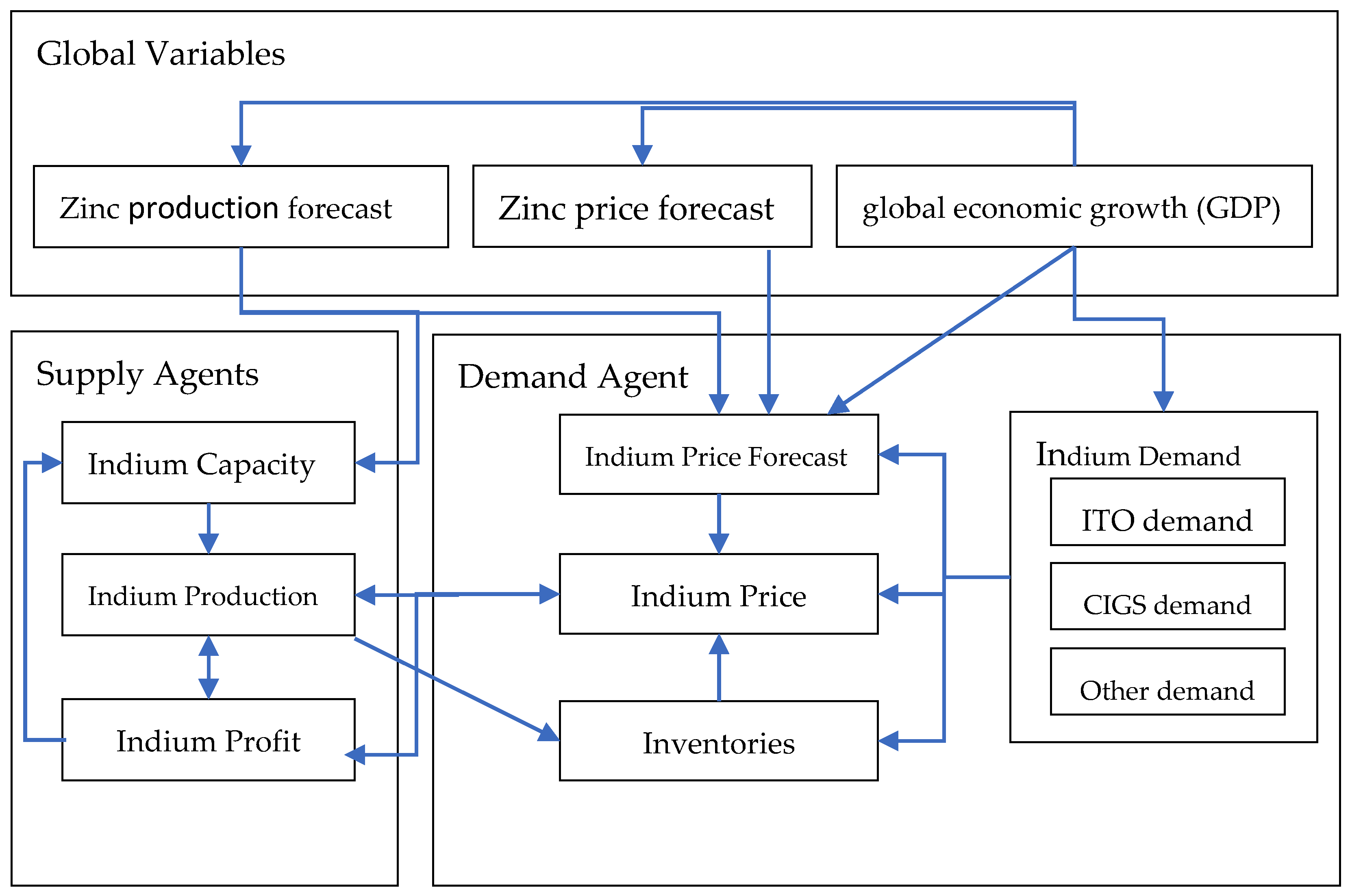
A total of 25 supply agents representing active indium metal producers listed by USGS indium minerals yearbook are included in the model [12]. A global demand agent is also created to manage demand, stock, and price changes. This agent represents a centralized indium market that adjusts global indium price based on supply–demand balance at each time step and exchanges decision-critical information with the rest of the model. The data dependency chart is shown in Figure 1.
The simulation starts at 2008, and the first 11 years are used as a warm-up period and for model validation. Since minimum resolution of indium data available is at annual level, the simulation time step is set to 1 year. The simulation ends at 2050. Specific agent behaviors and parameter setting are discussed in the following sections.
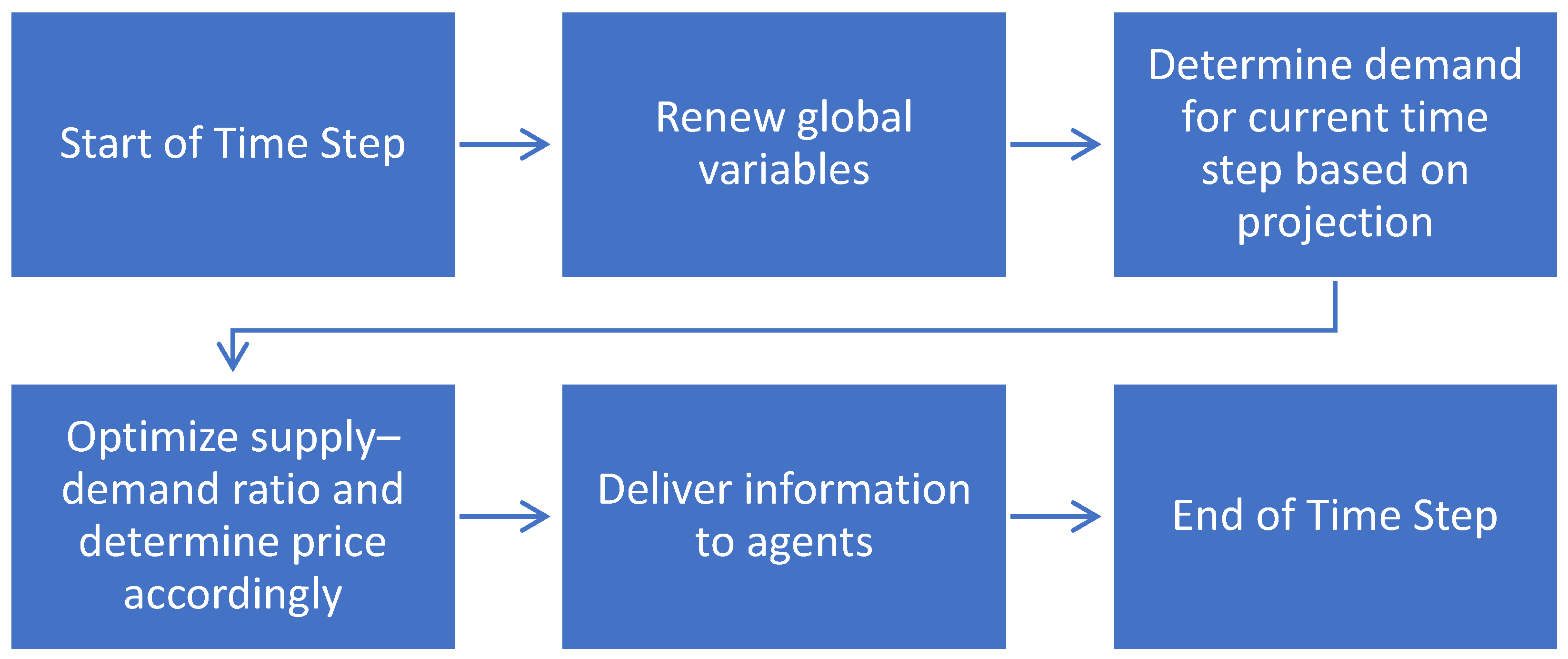
For each time step, global agent follows processes shown in Figure 2. Variables are first generated based on input data including zinc total production, projected zinc price, and GDP growth rate. After that, indium demand of current time step is generated, and a long-term indium price forecast is made based on zinc production, zinc price, indium demand, and economic growth rate. Indium capacity is also adjusted if a supply agent is zinc based and its zinc production changes. After that, a Cournot market competition problem for current time step is generated based on given data.
To ensure the existence of the Nash equilibrium, the model assumed a decreasing marginal revenue and an increasing marginal cost for all agents. The formulation for time step t is shown below:
where is the production of agent i at time t; is the total production of all other agents at time t; is the global price function at time t; is the cost function for agent i at time t; and is the production capacity for agent i at time t. This model assumes a quadratic production cost function and a fixed unit capital cost. Detailed parameter setting is listed in the Appendix A.
It is assumed that indium price is both influenced by long-term predictions and short-term supply–demand ratio. The price function can be formulated as follows:
where is the long-term predicted price and r is the current supply–demand ratio calculated by current production level , inventory level , and demand at time t. β > 0 is the impact parameter of supply–demand ratio over the price and is calibrated based on historical data. Long-term predicted price is based on input from historical data utilizing ARDL regression. The predicted price is determined by zinc production, zinc price, current indium demand, GDP growth, and indium price from previous years.
Once the Nash equilibrium problem is solved, the model calculates current global inventory level based on total production and demand, which is:
The model then continues to the next time step after agent behaviors are determined.
3.4. Indium Demand Projection
The demand projection is divided into three parts: ITO, CIGS, and others. ITO demand projection is assumed to follow a logistic curve based on year-wise deduction after 2018:
where the curve parameters K, G, and t0 are determined by non-linear regression from existing ITO production and projection data between years 2011 and 2020 [50]. Since the USGS report estimated ITO production has remained the same in recent years [12], the model assumes that the market is near a saturation state.
Meanwhile, a large amount of secondary indium is reclaimed by recycling ITO off target during the spurring process and is returned into ITO production loop. USGS assumed that a total of 1200 t/year of secondary indium was recovered from ITO recycling during 2016 [12]. However, based on the opinion from NREL, this number contains indium recovered from multiple loops [9]. Thus, calculation is conducted to determine the percentage of primary indium needed, which utilizes the same approach from NREL report. The ITO spurring loop data is shown in Table 1. A 30% efficiency for the spurring process and a 90% efficiency for the recovery process are assumed here [51].
As a result, to recover 1200 t of indium, 705.45 t of primary indium should be fed into the loop. Thus, a deduction factor of 2.70 is applied to total indium demand from ITO, indicating that only 37% of total indium consumption by ITO comes from primary production.
For CIGS demand, three different parameter sets are generated to represent different projections on thin-film solar PV market [52,53]. Historical data are then fed into the three scenarios to generate separate logistic demand curves similar to ITO demand. The parameters are listed in Table 2.
A layer thickness of 1.6 μm and efficiency at 11.2% in 2008 were previously reported [52]. The model assumes that these two parameters will shift linearly toward the 2020 assumption listed in the table under three different scenarios and then shift toward 2050 assumption under different rates. The report also gave an indium consumption estimate of 83 kg per GW of CIGS manufactured in 2008, which decreases accordingly due to reduce layer thickness and improve efficiency.
For other demands of indium, the simulation assumes that the demand remains constant at 2012 level as reported by NREL [9].
3.5. Supply Agent Behaviors
The supply agents include 25 primary indium producers listed by USGS, except for producers who have already terminated their operations [12]. Agents are assigned with several attributes. Detailed discussion on the value and deduction of such attributes is presented in the Appendix. Based on USGS information, there are three types of indium producers. Out of the 25 producers in the model, three agents produce indium based on primary metal other than zinc. Five agents produce indium from secondary source (mine residues, primary metal refinery residues, etc.) and purchase indium-containing materials from a third party. The remaining seventeen agents are zinc based.
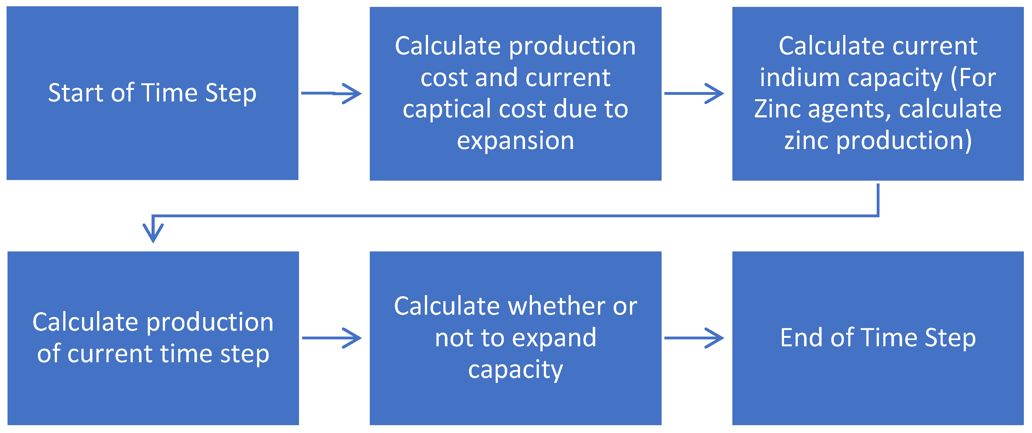
For each time step, supply agents make several decisions following the flow chart in Figure 3. First, the agents calculate any production cost and capital cost changes, either due to inflation or expansion. After that, zinc-based agents decide their zinc production of the current step. The total amount of zinc capacity taken into consideration by this study is only 1/3 of global primary zinc capacity [54]. The zinc market is therefore treated as a market with perfect competition and optimized accordingly [15]. The formulation of the optimization problem is listed as below:
where is the decision variable, which is the zinc production for zinc agent at current time step. is the input data of zinc price forecast at time [55], and is the individual zinc production cost mentioned above. is the increased marginal cost factor, and its value is estimated from reports. Zinc production capacity for each time step is calculated based on global zinc production forecast [56] and a fixed market share based on 2018 zinc production data [57].
Each agent calculates its actual indium capacity for each time step based on both facility capacity and indium content delivered to the facility. Non-zinc-based primary producers have their available indium raw material increasing each year in accordance with GDP growth. Zinc-based primary producers calculate their indium content based on zinc production and unit indium content of zinc-concentrate. Secondary producers have no indium content limit as they can always adjust the amount of raw material they bought.
The agents then decide whether they want to expand their indium production capacity by comparing possible profit against capital cost. The agent only expands their capacity if they have already utilized 90% of their current capacity. Total projected profit is calculated using a moving average of price in 3 years (pavg) and a deduction rate (rdiscount) of 8% [58] over a 10 year period. The agent solves the following local optimization problem:
where is the projected production, is the cost function, and one year of construction period is assumed based on refinery report [58]. is the unit expansion cost, is the maximum possible capacity calculated based on indium content, and is the capacity expanded. After an expansion, the expansion cost is averaged to a 10 year period as an increased fixed cost, and the indium capacity is increased after the construction period to reflect the expansion.
3.6. Validation and Verification
The verification and validation of agent-based model is vital [59]. Verification is to prove that the model itself is valid and correctly runs as intended, and validation is to prove that the model correctly and robustly reflects situations in the real world.
To verify the model, each subsystem of the model is tested individually to ensure that they work as proposed. Codes are carefully examined to ensure they work as intended. A dynamic test of the whole system with a different set of parameters is also conducted, which also serves as a sensitivity analysis for validation of the model.
To validate the model, several approaches are made. First, the model runs under a real-world dataset between 2007 and 2018, and several outputs are compared with the corresponding historical data. The result is shown in Table 3.
The model also runs under a set of extreme parameters, including large demand, zero demand, and a large stock. The extreme test was used to ensure that the model reflects correctly under such conditions.
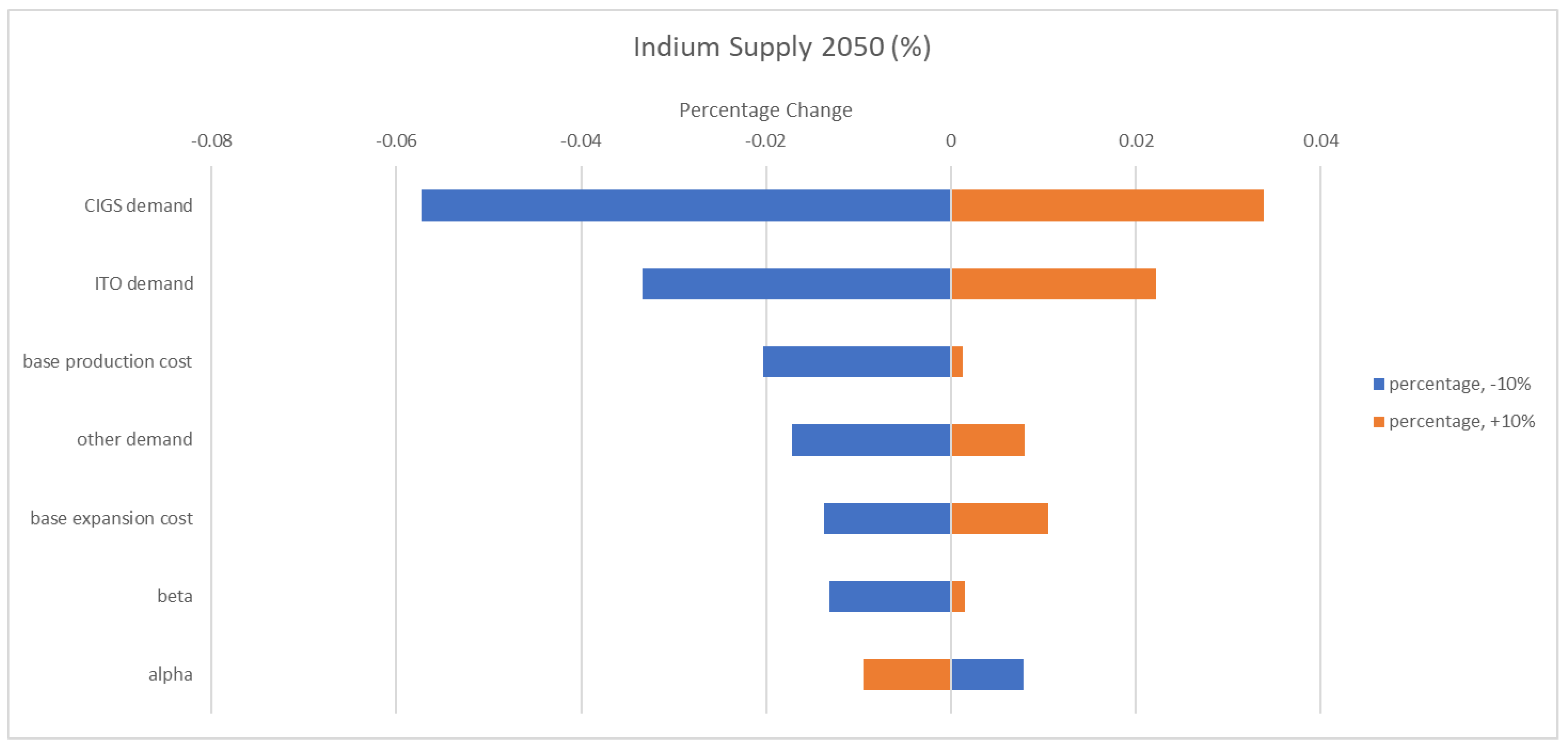
Finally, a sensitivity analysis is conducted to ensure the robustness of the model. The tornado graph of such analysis is shown in Figure 4.
Overall, the model correctly reflects historical production and price trends, while maintaining a good robustness considering parameter inaccuracy.
4. Results and Discussions
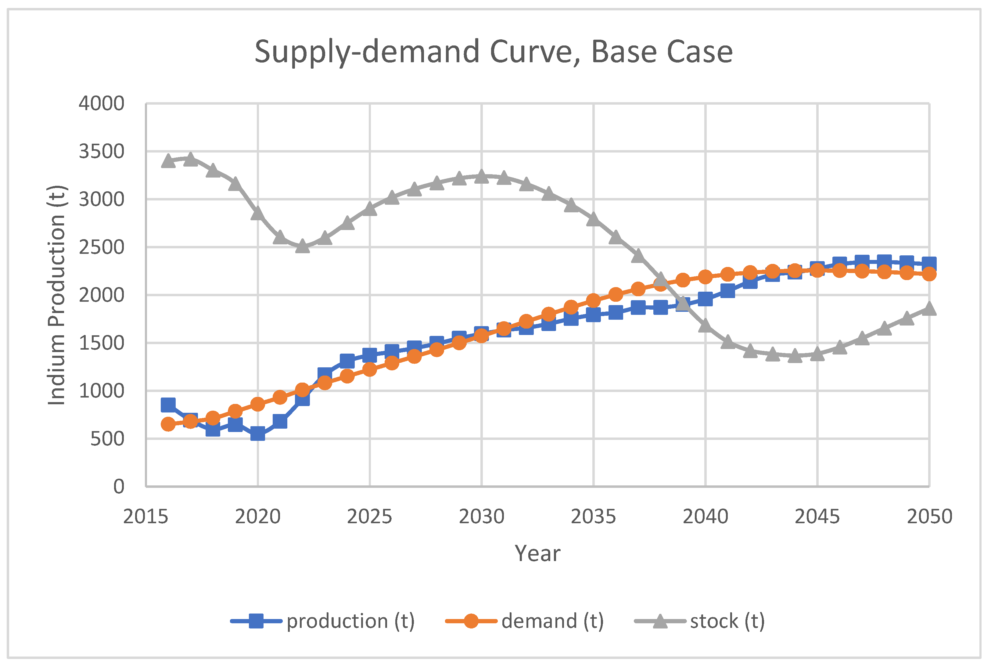
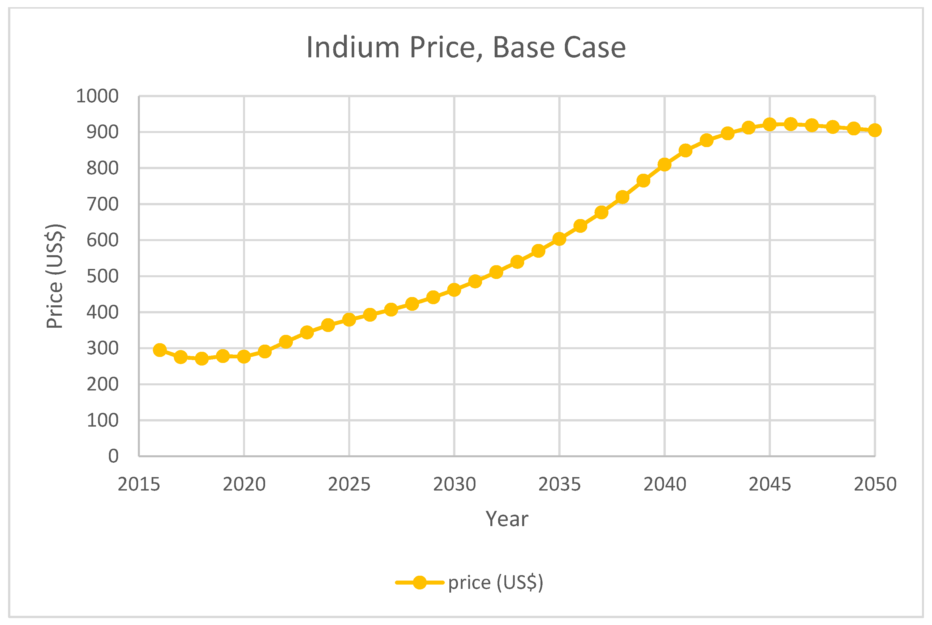
The result under the base case is shown in Figure 5, Figure 6 and Figure 7. Under the base case, the smelters are able to provide enough supply for future primary indium demand in a competitive market. With enough demand, the existing stock is gradually decreased to the level of annual indium production. Indium price is mostly pushed by the inflation rate, as the final price is equivalent to 452 $/kg in 2016 dollar. Although usually increasing, indium capacity decrease between years can be observed mainly due to decreased zinc primary production.
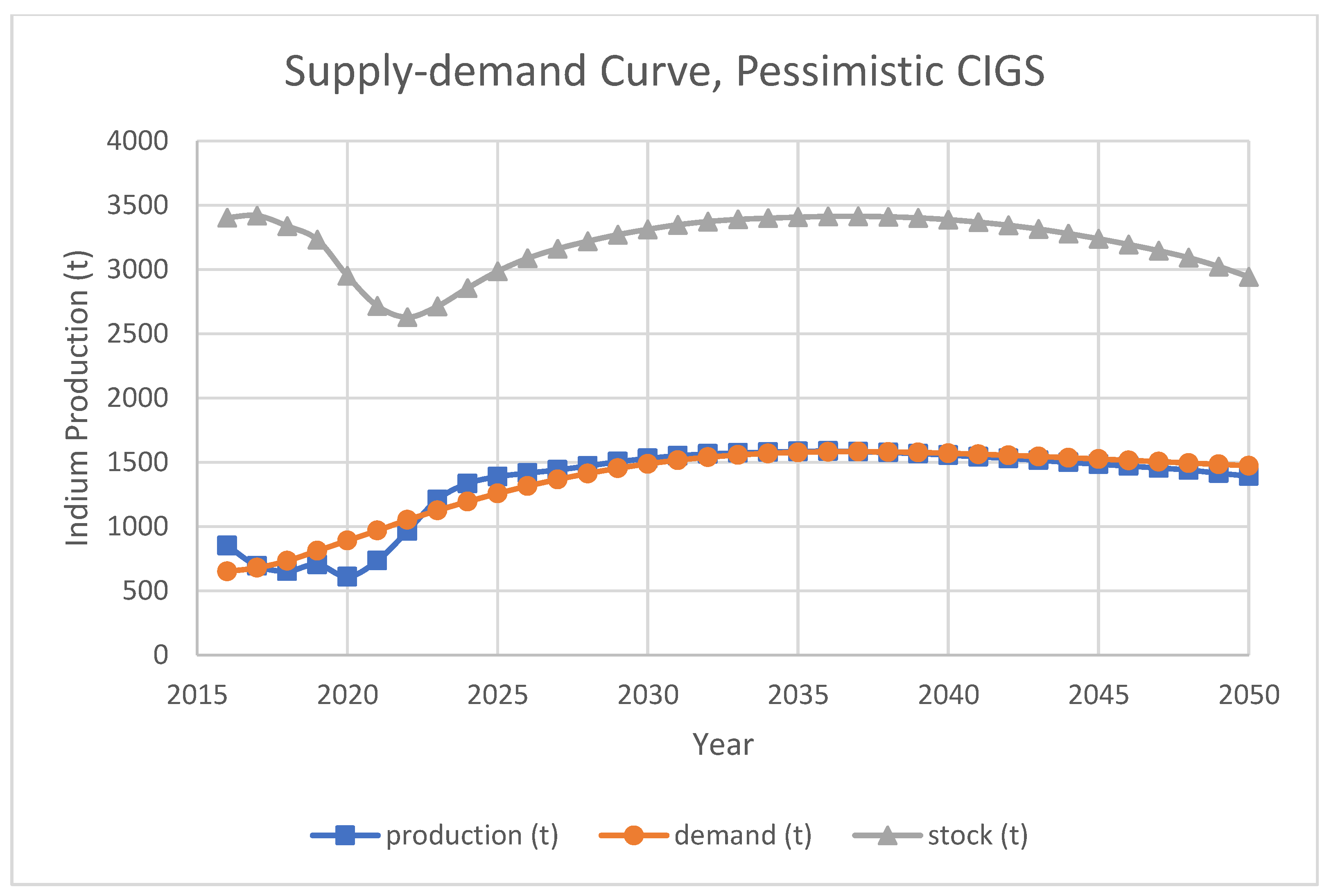
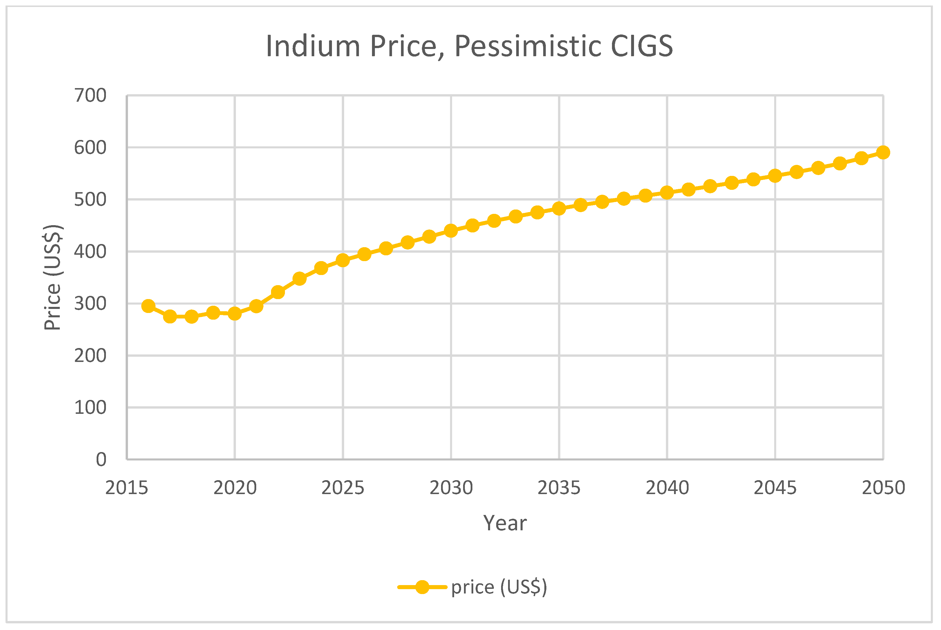
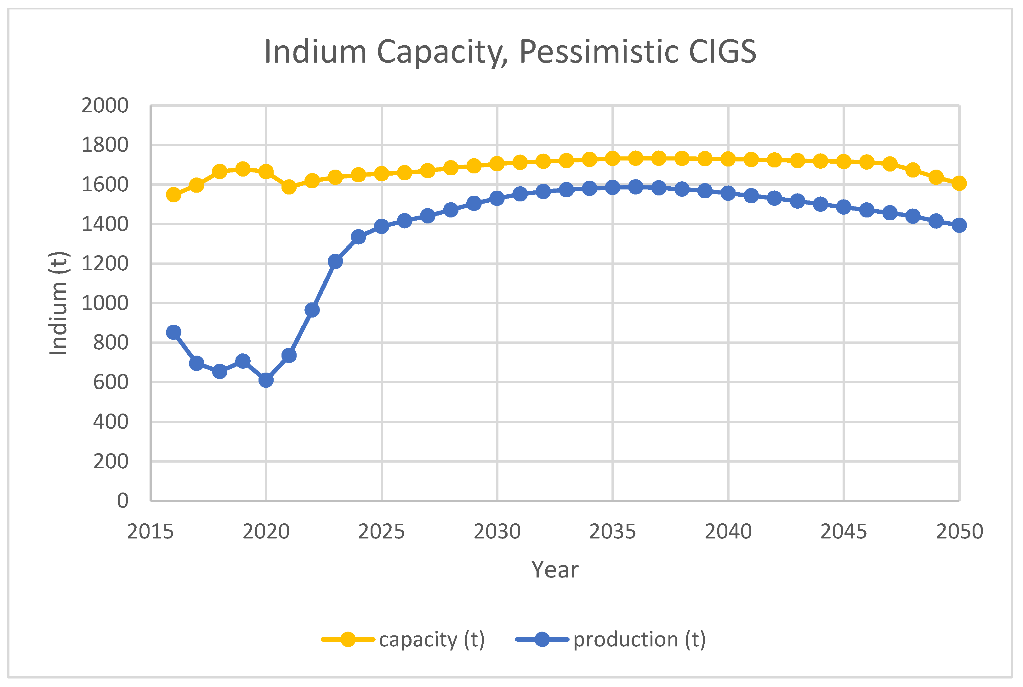
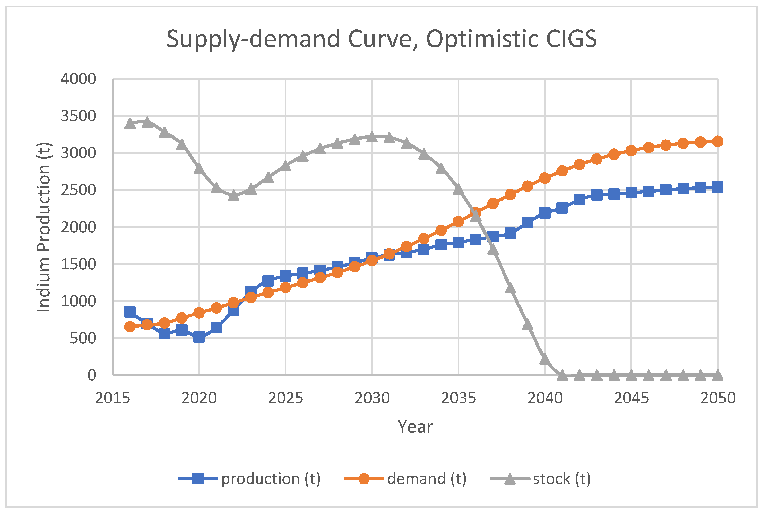
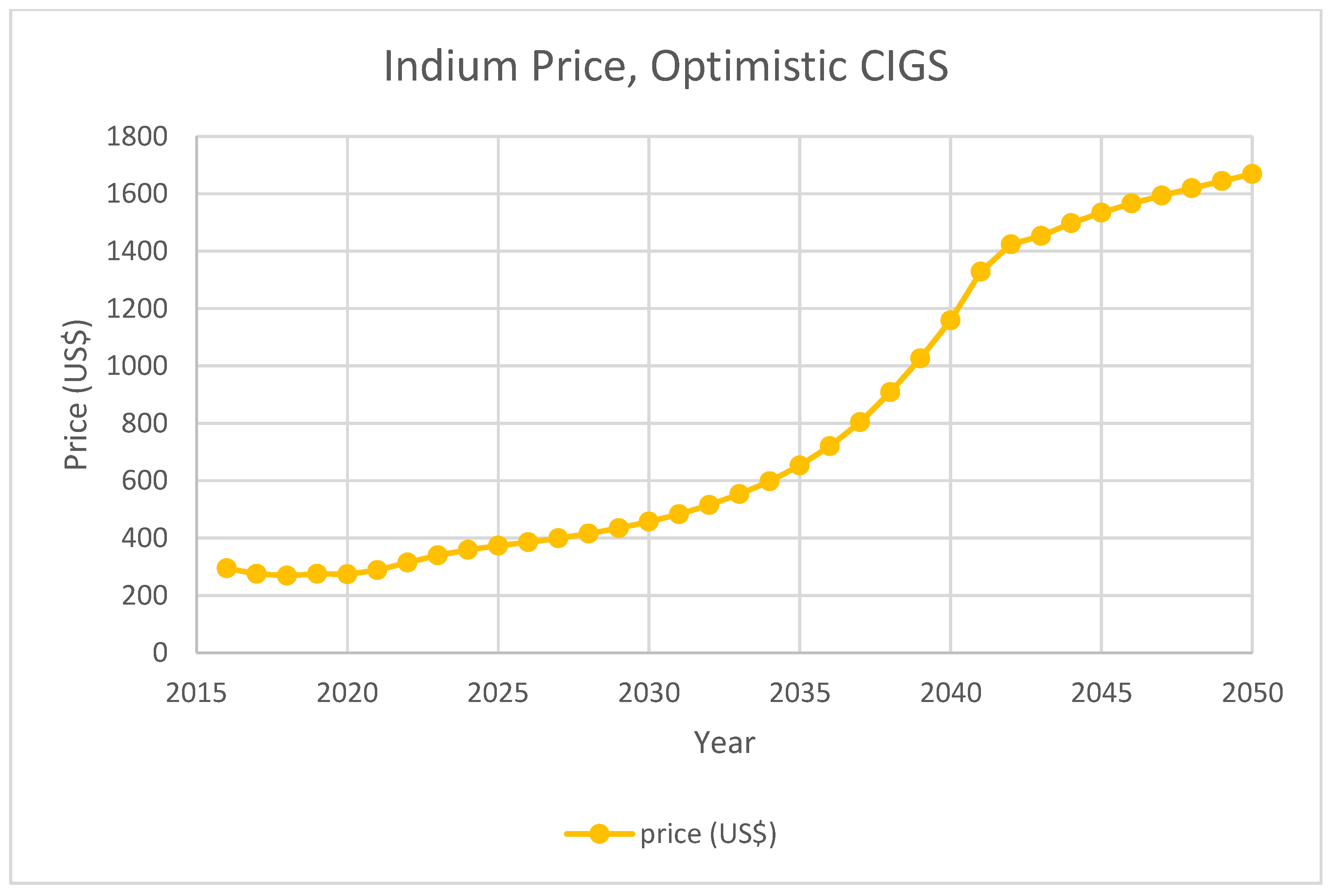
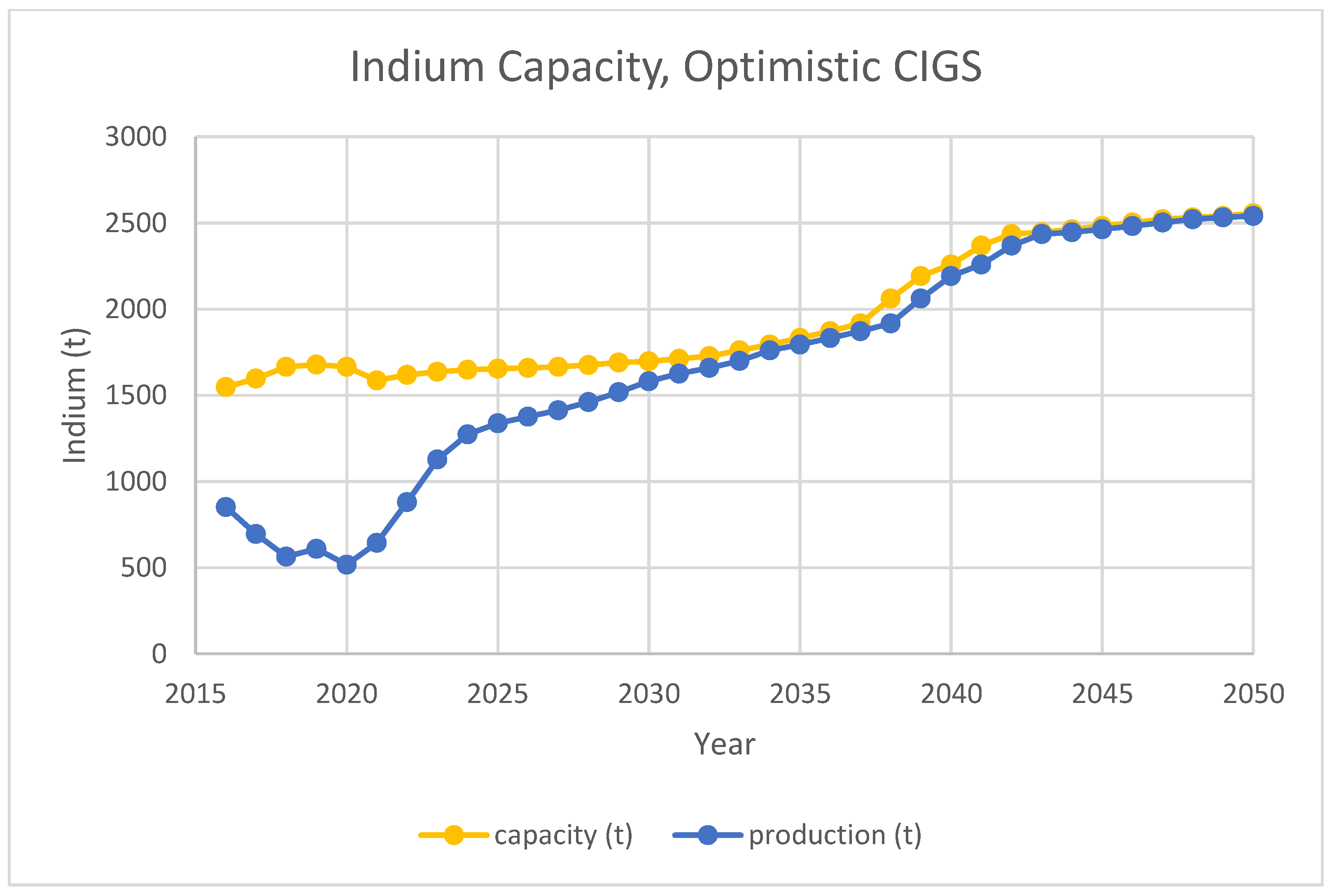
For pessimistic and optimistic CIGS projection scenarios, the results are shown in Figure 8, Figure 9, Figure 10, Figure 11, Figure 12 and Figure 13, respectively. The lack of demand increase in the pessimistic case makes it difficult for the high stock level to be consumed. As a result, indium price remains low. In addition, the capacity of indium smelters is not expanded as indium demand can already be satisfied. For the optimistic case, a supply deficiency is predicted after 2040. Although indium price is high, the expansion of current facilities is at their limit under current indium recovery rate.
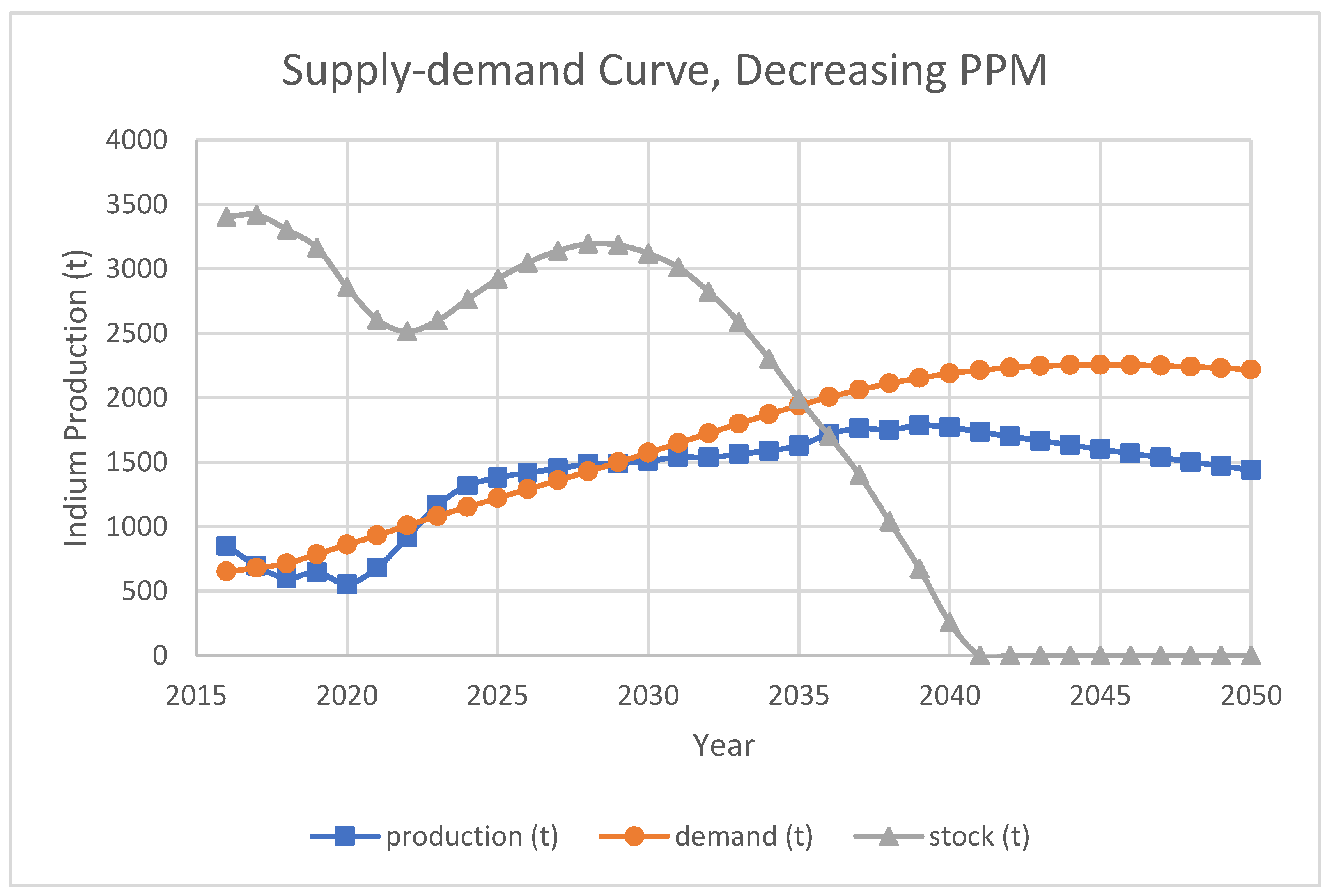
It is also interesting to see how indium extracting efficiency affects the supply. Two scenarios are set up to study such situations. The first scenario assumes that indium concentration in delivered ores starts to deteriorate over time. This scenario is established on the basis of the base-case scenario. This assumption follows Werner’s indium reserve assessment [20]. The assessment includes many indium-containing resources with low indium ppm. Thus, in this scenario, after the proposed current reported deposits of 76,000 t is consumed, the average indium ppm deteriorates linearly to 100 (reported minimum economic feasible value) until a total 356,000 t of indium is mined. This reduces the maximum indium capacities for smelters and raises unit production cost. An overall indium ore-to-metal efficiency of 17% is assumed following Lokanc et al.’s estimation [9].
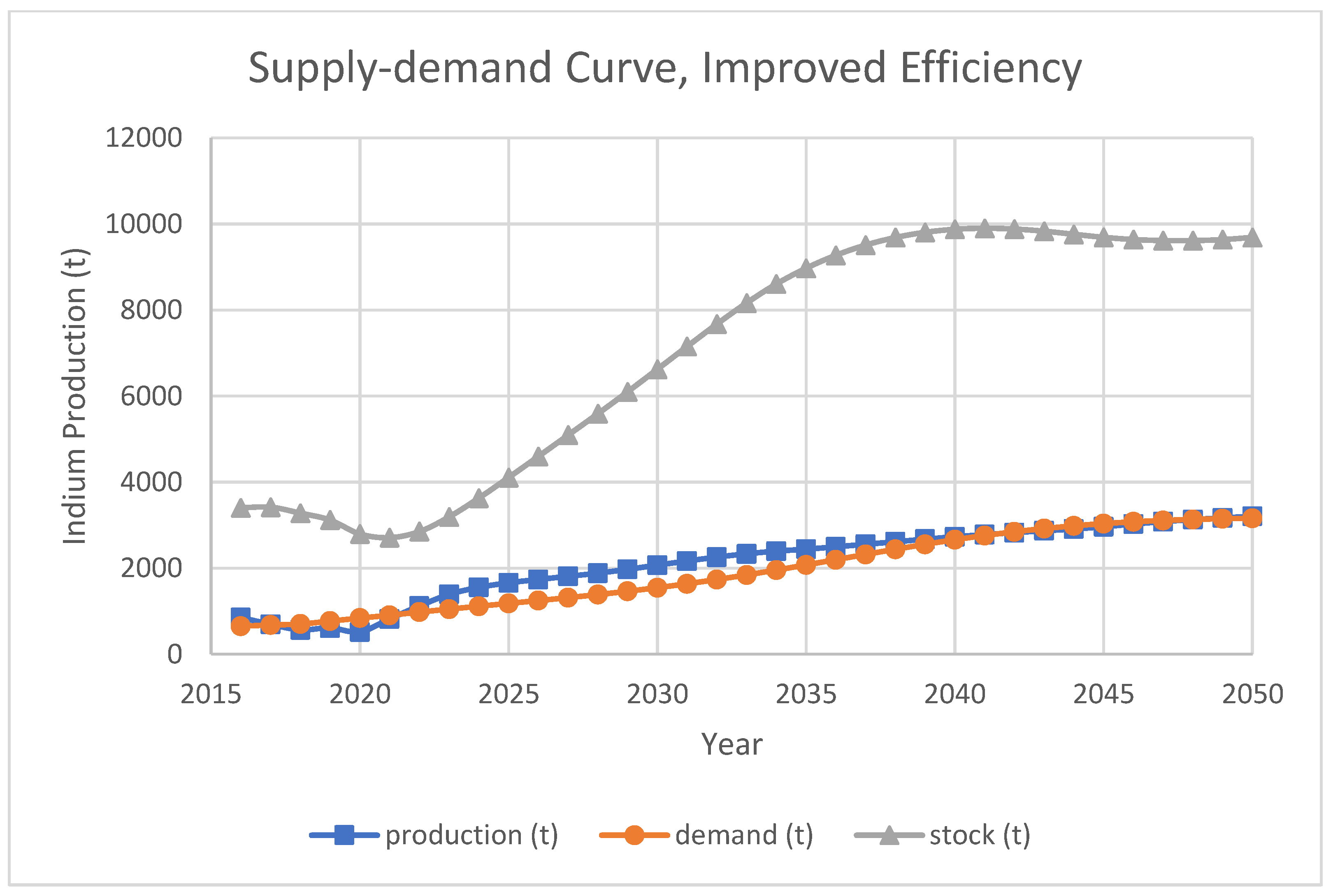
Another scenario assumes a possible indium recovery efficiency increase. This can include improved technology to recover more indium from ores into host-metal concentrates at mines, better recovery rate at smelters, or higher percentage of indium-containing concentrates sent to indium smelters. For the scenario setup, an efficiency of 68% is achieved at the end of simulation [9]. The efficiency increases linearly from 17% over time for each smelter after 2020. This increases the maximum indium capacity for smelters. The unit production costs for the smelters are also reduced. To better reflect the result, this scenario is set up based on optimistic CIGS scenario, where a supply shortage happens.
The results for both scenarios are shown in Figure 14, Figure 15, Figure 16 and Figure 17, respectively. It is apparent that efficiency of smelters is vital to indium supply. If the primary supply of indium-containing ore could not maintain current quality, supply shortage occurs. Meanwhile, improvements on indium overall efficiency are extremely effective, and indium supply with improved efficiency is sufficient to meet the optimistic CIGS projection demand.
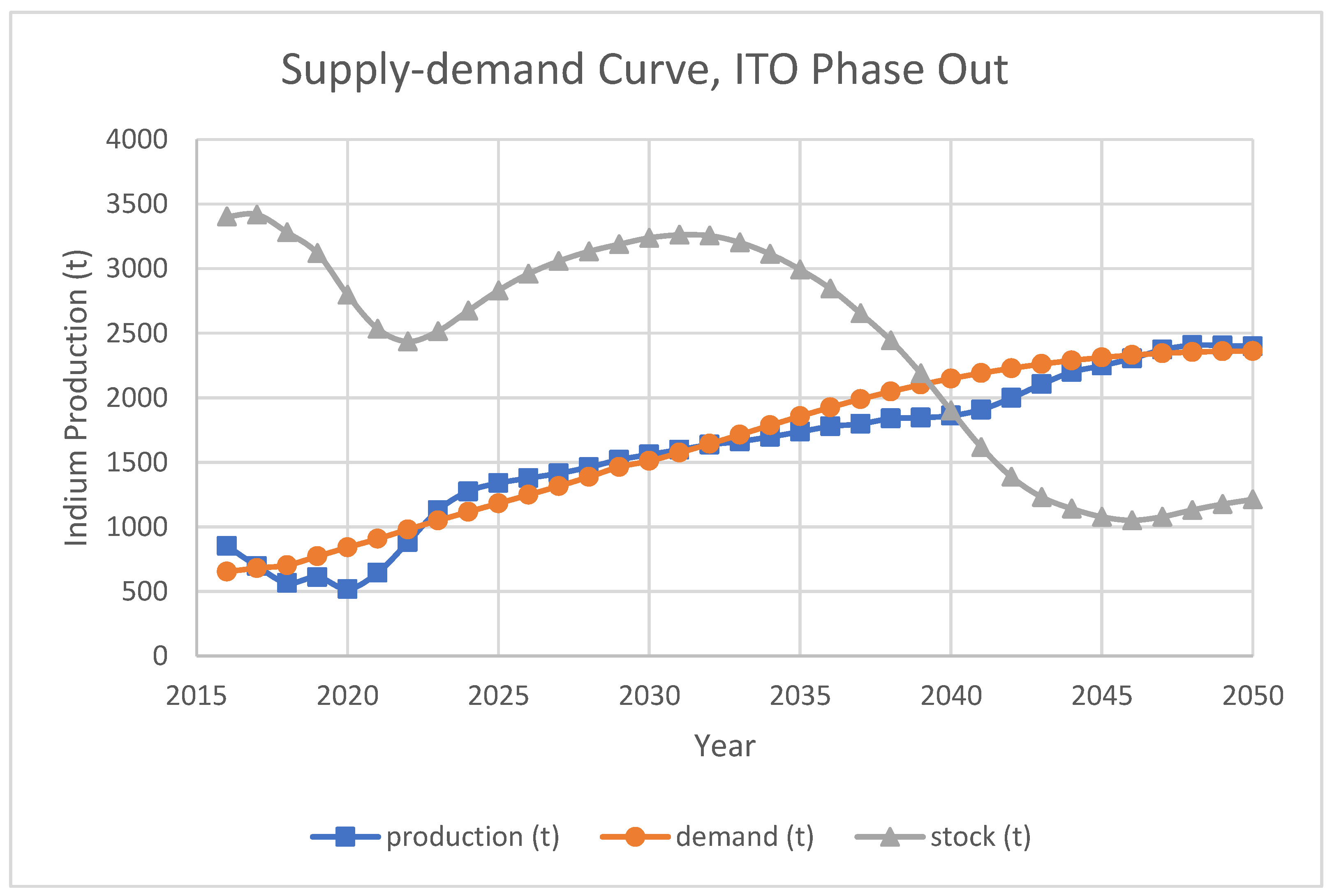
Another possible scenario would be the phase out of ITO technology. Since ITO might be substituted with carbon nanotube and graphene (Bernhardt, 2019), in this scenario, an ITO phase out will start happening at 2025 following a reversed S-curve. The result based on optimistic CIGS case is shown in Figure 18. A more apparent supply shortage is observed around 2040. Due to the phase out of ITO, the producers are not fully expanding their capacities until more demand from CIGS emerges, which causes temporary shortage before indium price is raised to attract facility expansion.
The above simulation result shows several interesting trends. The competition between producers helps to stabilize indium price at the cost of supply–demand gaps. The producers are unwilling to utilize full indium production capacities at a lower price even if there is surplus demand. Meanwhile, when the market is relatively stable, the production roughly meets the demand. Moreover, it may not be profitable for producers to continually expand indium production due to increasing marginal cost for indium production under this model.
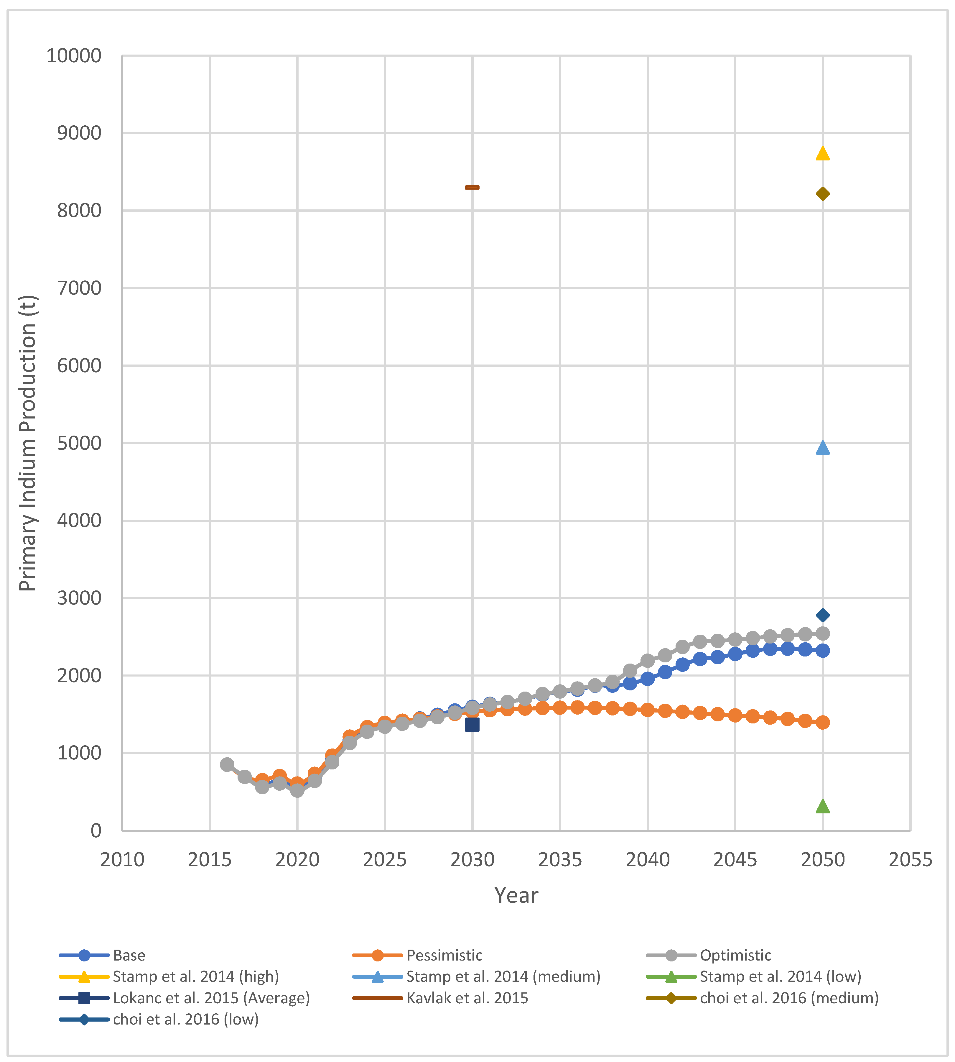
The primary supply result from this research is also compared with previous predictions on indium demand, as shown in Figure 19. The demand outlooks from different research vary mainly because of different CIGS market penetrations. Under most cases, there is a gap between primary indium supply predicted by this model and predicted indium demands from other research. Part of the gap can be filled with secondary indium supply, mainly from in-process ITO production, which is roughly 1400 t by the end of simulation. However, for even higher indium demand penetration, as shown in the optimistic CIGS case from this research, it may be difficult to fulfill the gap solely with primary indium production.
5. Conclusions and Future Research
Overall, this work established a competitive oligopolistic indium metal market model based on Cournot equilibrium using agent-based modeling method. Under base-case and low CIGS demand case of the model, supply–demand balance can be maintained by current market suppliers. However, if faced with higher demand from CIGS manufacturing, current suppliers are not willing to continue expanding their indium production due to increased marginal cost even with a supply shortage. There is also a delay between increased demand and increased indium capacities. The suppliers often wait until indium price is high enough before they expand their indium capacities. This can also cause temporary supply shortage. As a conclusion, the economic concerns of indium producers largely influence the indium supply–demand balance.
On the other hand, the availability of raw material with high indium concentration is vital to indium supply. If unit indium production costs increase due to the deterioration of raw material, the producers would not be willing to expand their production but rather try to maintain a high indium price to compensate the increased cost. A way to reduce such costs is to increase overall indium recovering efficiency, but it may require additional research and capital costs, which is not modeled in this work.
Current base model assumes that smelters can always acquire sufficient raw materials. However, this may not be true. As reported by Werner et al., current indium primary resource inferred is 356,000 t [20]. Although this seems sufficient to support demand described by the model, economic feasibility of each site for indium remains questionable.
Current work did not include other layers of indium supply chain. Important questions regarding indium-containing ores—if they hold sufficient indium, economic feasibility in their recovery, and complementary sources of indium supply—are still left unanswered.
Another possible source of indium supply is the recycling of end-of-life indium products. Currently, recycling mainly happens within the ITO production cycle. For end-of-life recycling, flat panel display is projected to be the largest source, for which cost-effective recycling methods are currently being developed [61]. According to the current literature review, ITRI technology developed a pilot recycling system with a cost of $2000 per ton of e-scrap processed [62]. However, only 750 grams of indium can be extracted from 1 ton of waste flat panel display, and the profit of indium is the lowest comparing to other products. Thus, indium is still a by-product in the end-of-life recycling process. As discussed prior, CIGS waste flow will become significant in the future since the average lifespan of current product is about 10–15 years [63].
Author Contributions
Conceptualization, J.C. and F.Z.; methodology, J.C. and C.H.C.; software, J.C.; validation, J.C. and C.H.C.; formal analysis, J.C.; investigation, J.C. and C.H.C.; resources, J.C. and C.H.C.; data curation, J.C. and C.H.C.; writing—original draft preparation, J.C.; writing—review and editing, F.Z.; visualization, J.C. and C.H.C.; supervision, F.Z.; project administration, F.Z.; funding acquisition, F.Z. All authors have read and agreed to the published version of the manuscript.
Funding
This research is funded by the Critical Materials Institute, an Energy Innovation Hub funded by the U.S. Department of Energy, Office of Energy Efficiency and Renewable Energy, Advanced Manufacturing Office. The APC was funded by the Critical Materials Institute.All data presented in this study are available in corresponding publicly accessible sources. All data sources are referenced individually.
Conflicts of Interest
The authors declare no conflict of interest.
Appendix A. Detailed Model Formulation
Appendix A.1. Global Parameters and Variables
Global parameters are input parameters from outside of the model and are applied to each agent including demand agent and indium producer agents. Detailed description of each parameter is listed in Table A1. Average CPI and GDP growth are assumed based on respective values for recent years [64,65]. Indium primary production cost quadratic factor and indium price elasticity are calibrated by running the model from 2008 to 2018 with different parameter pairs . Modeled indium primary production and modeled indium price are compared with historical production and price data. Parameter pairs with least normalized squared error are selected as final model parameters.

Table A1.
Global parameters.
| Parameter Name | Description | Data Source |
|---|---|---|
| Indium primary production cost quadratic factor () | Quadratic factor for indium primary production cost function. | Calibrated [8,44,58] |
| Indium price elasticity () | Indium price change factor in response to supply–demand ratio | Calibrated [44] |
| GDP (GDP) | Global GDP annual nominated growth. (Data before 2020 are historical growth) | [64] Assumption |
| Inflation (CPI) | Most cost increases proportionally by inflation rate each time step. | [65] Assumption |
| Predicted zinc production () | Predicted total annual primary zinc production. (Data before 2020 are historical data) | [56,57] |
| Predicted zinc price () | Predicted zinc price. (Data before 2020 are historical data, prediction extended from 2030 to 2050) | [55] |
Global variables are variables aggregated among agents each time step. Detailed description of each variable is listed in Table A2. Global inventory each step is calculated by the following equation:
Indium primary production at time step is calculated by the sum of primary production from all indium supply agents:
Indium demand at time step is calculated by the sum of ITO demand, CIGS demand, and other demand:
Indium long-term predicted price at time step is calculated by the following regressed equation:
Table A2.
Global variables.
| Variable Name | Description | Data Source |
|---|---|---|
| Inventory () | Global indium inventory level at time t. Initial value equals to 2008’s total primary production capacity. | [12] |
| Indium primary production () | Annual total indium primary production at time t. Initial value equals to 2008’s total primary production capacity. | [12] |
| Indium predicted price () | Long-term prediction of indium price based on ARDL regression at time t. | [44,55,57,60] |
| Indium price () | Modeled indium price after competition at time t. Initial value equals to 2008’s historical price. | [60] |
| Indium demand () | Modeled indium primary demand at time t. Initial value equals to 2008’s historical primary demand. | [44] |
| Supply–demand ratio ( | Modeled supply–demand ratio at time t. | Calculated |
The long-term predicted price is regressed using corresponding data between 1974 and 2017 with ARDL regression [17]. The long-term predicted price explains most variance of the data (R-squared 0.74). Short-term supply–demand ratio is also an important factor to the market price [42]. Due to lack of data, it is not possible to include supply–demand ratio into long-term regression. Instead, the model calibrated the impact factor as mentioned before. Final indium market price is calculated as a function of total production and supply–demand ratio:
where supply–demand ratio is calculated by:
Appendix A.2. Demand Agent Parameters and Variables
Input parameters for indium demand prediction is listed in Table A3.
Table A3.
Demand agent parameters.
| Parameter Name | Details | Data Source |
|---|---|---|
| ITO recycling factor () | Ratio between total ITO demand and ITO primary production | Calculated [9] |
| ITO indium content factor () | Indium content in ITO | Calculated by molecular weight [66] |
| ITO demand logistic parameters () | Logistic curve parameters regressed using historical and prediction data | Assumption [12,50] |
| CIGS efficiency 2008 () | Known CIGS module energy efficiency by 2008 | [52] |
| CIGS indium layer thickness 2008 (μm) () | Known CIGS module indium-contained layer thickness by 2008 | [52] |
| CIGS indium content () | Indium content (t) per MW of CIGS installation, with indium layer thickness of 1.6 μm | [6,13,52,53] |
| CIGS scenarios parameters | See Table A1, Table A2, Table A3 and Table A4 Logistic curve parameters regressed using historical and prediction data | |
| Other indium demand () | Demand from other minor indium applications | [9,12,44] |
ITO recycling factor is calculated as described in the Model Formulation section of the article. ITO demand logistic parameters are the parameters of the logistic growth function, defined as:
where is the total ITO demand at time t. The parameter , which is the saturated market size of ITO, is assumed based on the prediction from USGS and ResearchInChina [12,50], with an additional 20% relaxation for a higher estimation of ITO demand. The other two parameters are then regressed based on historical ITO demand data calculated from historical primary indium demand data for ITO, with the recycling factor and indium content factor taken into consideration. Thus, total ITO demand projection each year can be generated by the function.
Meanwhile, since CIGS is an evolving technology, its material efficiency and energy efficiency will be improved over time. The decrease in indium-contained layer thickness and increased photovoltaic efficiency results in decreased indium consumption per GW of CIGS installation. To reflect this fact, based on the prediction from DOE and recent CIGS photovoltaic development information on market share and lab energy efficiency, three scenarios based on different technology projection are developed [6,52,53]. Here, final technological advancement by 2050 on layer thickness and energy efficiency for all scenarios are the same. Layer thickness follows the data from DOE projection, and energy efficiency follows the latest reported lab efficiency. On the other hand, different advancement speed and market projection are selected for each scenario. Advancement speed is based on the scenarios provided by DOE projection [13,52]. Market size projection by 2050 are calculated from market share projection from latest photovoltaic report and total solar power generation market size [13,53]. Similarly, a logistic growth function is then regressed based on historical CIGS production and final CIGS market size for each scenario, from which CIGS annual installation projection for each scenario is generated.
Finally, indium consumption from other minor usages is modeled as constant either because the application is a long-existing one with a saturated market, or the application does not consume significant amount of indium, as discussed in the article.
Demand agent variables are described in detail in Table A4. Primary indium demand from ITO at time t is calculated based on logistic function for annual total ITO demand as:
where total ITO demand is firstly deducted by recycling factor to determine ITO produced from primary indium, and primary indium consumption is then calculated by applying ITO indium content factor.
Table A4.
Demand agent variables.
| Variable Name | Details | Data Source |
|---|---|---|
| ITO indium demand () | Predicted primary indium demand from ITO at time t. | Logistic curve parameters regressed |
| CIGS efficiency () | Linearized yearly result for CIGS efficiency under corresponding scenario | Calculated |
| CIGS indium layer thickness () | Linearized yearly result for indium-contained layer thickness in CIGS under corresponding scenario | Calculated |
| CIGS indium demand () | Predicted primary indium demand from CIGS at time t. | Logistic curve parameters regressed |
| Total indium demand () |
The model assumed that CIGS technology advancement is linear between scenario-wise checkpoints. For example, under the base case, layer thickness changes linearly between 2008 and 2020, from 1.6 to 1.0 μm and then follows another linear change between 2020 and 2050, from 1.0 to 0.8 μm. Primary indium demand from CIGS at time t is similarly calculated based on logistic function for annual CIGS installation in GW as:
Finally, total indium demand is calculated by:
To ensure that the uncertainties of model data and assumption do not impact model result too much, an uncertainty analysis has been conducted, as described in the Validation and Verification section of the article.
Appendix A.3. Supply Agent Parameters and Variables
Input parameters for each supply agent is listed in Table A5.
Table A5.
Supply agent parameters.
| Parameter Name | Details | Data Source |
|---|---|---|
| Indium capacity, 2016 () | Indium capacity for supply agent i at 2016 | [12] |
| Initial indium capacity factor () | Factor converting indium capacity of 2016 into 2008 | Assumption [60] |
| Average indium content in respect of host metal content (ppm) () | Average indium content in zinc concentrates that are processed by indium refineries | [9] |
| Manufacturing cost index () | Relative manufacturing cost between different countries, US=100 | [67] |
| Discount rate () | [58] | |
| Indium reference variable cost () | Indium production unit variable cost from refinery report | [8] Converted to 2008 dollar |
| Indium reference fixed cost () | Indium production unit fixed cost from refinery report | |
| Indium reference expansion cost () | Indium production unit capital cost over 10 years from refinery report, used as unit expansion cost | |
| Indium refinery efficiency () | Overall indium refinery efficiency to recover indium metal from zinc concentrates | [8] |
| Zinc refinery efficiency (Zinc agents only) () | Zinc refinery efficiency to recover zinc metal from zinc concentrates | [58] |
| Zinc market factor (Zinc agents only) () | The marginal cost factor of increased zinc production. Calculated from two refinery reports | Calculated [8,14,58] |
| Zinc reference cost (Zinc agents only) () | Zinc production base cost, calculated from two refinery reports | |
| Indium residue price factor () | Indium-containing residue material cost, modeled as percentage of current indium price | [58] |
Indium capacity for each agent at the beginning of simulation is assumed to have same proportion as 2016, thus the initial capacity for agent can be calculated as:
As described in the article, zinc market is formulated as a perfect market. Based on two known refinery reports from Canada and China with different zinc production capacity and cost, marginal cost factor and base cost are assessed by exponential regression with marginal cost formulation as:
Here, all cost data are normalized into U.S. dollar 2008 with MCI of 96 (China).
Indium supply agents are divided into three categories. Three agents produce indium based on host metal other than zinc. Five agents produce indium from secondary sources (mine residues, primary metal refinery residues, etc.) and purchase indium-containing raw materials. The remaining seventeen agents are zinc based. Detailed information is provided in Table A6. Several smelters listed by USGS are already terminated, thus excluded from the model.
Table A6.
Supply agent details.
Do., do. Ditto.
All variables used to model supply agents are presented in Table A7. For each time step, current indium maximum capacity is firstly calculated. This represents maximum possible indium-containing raw material available to each agent and is calculated as:
The initial value of for non-zinc-based primary agents are equal to their initial capacity . The initial value of for zinc-based primary agent j is calculated as:
For zinc-based agents, current zinc production capacity is modeled as:
Based on perfect market competition [14], each zinc-based agent j can be optimized separately by the following optimization problem:
Here, , and .
Once solved, current indium capacity for agent i can be represented as:
Meanwhile, the cost function of agent i at time t is modeled as:
The quadratic function is formulated so that it fits the known production cost from refinery report (Gu, 2006) with 20 t of annual indium production.
Here, , ,
, and
is the total expansion cost for current time step t, which is formulated as:
After all parameters are determined, the Nash equilibrium problem can be formulated as:
Here,
This is a potential game and can be solved using the best-response scheme.
Finally, each agent needs to consider about indium capacity expansion if they utilize up 90% of current capacity. This process is conducted via solving the following heuristic local optimization problem for from Canada refinery report [58]:
Here, is the indium price average in the recent 3 years,
and .
Table A7.
Supply agent variables.
| Variable Name | Details | Data Source |
|---|---|---|
| Indium capacity () | Indium capacity for supply agent i at time t | Initial value |
| Indium maximum capacity () | Maximum possible indium capacity for supply agent i at time t | |
| Indium production () | Indium production decision variable for supply agent i at time t | |
| Indium production expansion () | Indium production capacity expansion decision variable for supply agent i at time t | |
| Indium variable cost () | Indium production variable cost parameter for supply agent i at time t | |
| Indium fixed cost () | Indium production unit fixed cost for supply agent i at time t | |
| Indium expansion cost () | Indium production unit capital cost for supply agent i at time t over 10 years | |
| Indium total expansion cost () | Indium total expansion cost for supply agent i at time t, formulated as additional fixed cost | |
| Zinc production base cost (Zinc agents only) () | Zinc marginal cost parameter for zinc-based supply agent j at time t | |
| Zinc production (Zinc agents only) () | Zinc production decision variable for zinc-based supply agent j at time t | |
| Zinc capacity (Zinc agents only) () | Zinc capacity for zinc-based supply agent j at time t | |
| Indium content in respect of zinc content (Zinc agents only) () | Indium content density in respect of zinc content for zinc-based supply agent j at time t |
References
- Dudley, B. BP Statistical Review of World Energy; BP Statistical Review: London, UK, 2019. [Google Scholar]
- Kutak, R. Examination of Federal Financial Assistance in the Renewable Energy Market; Office of Nuclear Energy: Washington, DC, USA, 2018.
- Chu, S. (Ed.) Critical Materials Strategy; DIANE Publishing: Darby, PA, USA, 2011. [Google Scholar]
- Moss, R.L.; Tzimas, E.; Willis, P.; Arendorf, J.; Thompson, P.; Chapman, A.; Morley, N.; Sims, E.; Bryson, R.; Peason, J. Critical Metals in the Path towards the Decarbonisation of the EU Energy Sector. Assessing Rare Metals as Supply-Chain Bottlenecks in Low-Carbon Energy Technologies; JRC Report EUR; European Commission: Brussels, Belgium, 2013; p. 25994. [Google Scholar]
- Nassar, N.T.; Graedel, T.E.; Harper, E.M. By-product metals are technologically essential but have problematic supply. Sci. Adv. 2015, 1, e1400180. [Google Scholar] [CrossRef] [Green Version]
- Bleiwas, D.I. Byproduct Mineral Commodities Used for the Production of Photovoltaic Cells; US Department of the Interior, US Geological Survey: Reston, VA, USA, 2010.
- Mikolajczak, C. Availability of Indium and Gallium; Indium Corporation of America: Clinton, NY, USA, 2009. [Google Scholar]
- Gu, C.; Huang, S.; Cao, H.; Tan, H.; Liang, X.; Jiang, Z.; Nandan Country Jilang Indium Manufacturing Co., Ltd. Integrated Indium and Zinc Recovery Project Environmental Impact Statement; Scientific Research Academy of Guangxi Environmental Protection: Guangxi, China, 2006. [Google Scholar]
- Lokanc, M.; Eggert, R.; Redlinger, M. The Availability of Indium: The Present, Medium Term, and Long Term; No. NREL/SR-6A20-62409; National Renewable Energy Lab. (NREL): Golden, CO, USA, 2015. [Google Scholar]
- Bernhardt, D.; Reilly, J.F., II. Mineral Commodity Summaries 2019; US Geological Survey: Reston, VA, USA, 2019.
- Du, Y.; Hu, Y.; Lei, X. Analysis of the supply and demand trend of indium and recommended management strategies. China Min. Mag. 2016, 25, 33–34, 64. [Google Scholar]
- Anderson, C.S. Indium. In Minerals Yearbook—Metals and Minerals; Advance Release 2016; U.S. Geological Survey: Reston, VA, USA, 2019. [Google Scholar]
- Dhabi, A. Global Energy Transformation: A Roadmap to 2050, 2019th ed.; International Renewable Energy Agency, IRENA: Abu Dhabi, United Arab Emirates, 2019. [Google Scholar]
- Fizaine, F. Byproduct production of minor metals: Threat or opportunity for the development of clean technologies? The PV sector as an illustration. Resour. Policy 2013, 38, 373–383. [Google Scholar] [CrossRef]
- Afflerbach, P.; Fridgen, G.; Keller, R.; Rathgeber, A.W.; Strobel, F. The by-product effect on metal markets–new insights to the price behavior of minor metals. Resour. Policy 2014, 42, 35–44. [Google Scholar] [CrossRef]
- Redlinger, M.; Eggert, R. Volatility of by-product metal and mineral prices. Resour. Policy 2016, 47, 69–77. [Google Scholar] [CrossRef] [Green Version]
- Fu, X.; Polli, A.; Olivetti, E. High-Resolution Insight into Materials Criticality: Quantifying Risk for By-Product Metals from Primary Production. J. Ind. Ecol. 2019, 23, 452–465. [Google Scholar] [CrossRef]
- Mudd, G.M.; Jowitt, S.M.; Werner, T.T. The world’s by-product and critical metal resources part I: Uncertainties, current reporting practices, implications and grounds for optimism. Ore Geol. Rev. 2017, 86, 924–938. [Google Scholar] [CrossRef]
- Werner, T.T.; Mudd, G.M.; Jowitt, S.M. The world’s by-product and critical metal resources part II: A method for quantifying the resources of rarely reported metals. Ore Geol. Rev. 2017, 80, 658–675. [Google Scholar] [CrossRef]
- Werner, T.T.; Mudd, G.M.; Jowitt, S.M. The world’s by-product and critical metal resources part III: A global assessment of indium. Ore Geol. Rev. 2017, 86, 939–956. [Google Scholar] [CrossRef]
- Kavlak, G.; McNerney, J.; Jaffe, R.L.; Trancik, J.E. Metal production requirements for rapid photovoltaics deployment. Energy Environ. Sci. 2015, 8, 1651–1659. [Google Scholar] [CrossRef] [Green Version]
- Nassar, N.T.; Wilburn, D.R.; Goonan, T.G. Byproduct metal requirements for US wind and solar photovoltaic electricity generation up to the year 2040 under various Clean Power Plan scenarios. Appl. Energy 2016, 183, 1209–1226. [Google Scholar] [CrossRef]
- Stamp, A.; Wäger, P.A.; Hellweg, S. Linking energy scenarios with metal demand modeling—The case of indium in CIGS solar cells. Resour. Conserv. Recycl. 2014, 93, 156–167. [Google Scholar] [CrossRef]
- Jackson, W.; Director, T.F.; Unit, S.B. The Future of Indium Supply and ITO; Indium Corporation: Clinton, NY, USA, 2012. [Google Scholar]
- Candelise, C.; Winskel, M.; Gross, R. Implications for CdTe and CIGS technologies production costs of indium and tellurium scarcity. Progress Photovolt. Res. Appl. 2012, 20, 816–831. [Google Scholar] [CrossRef]
- Choi, C.H.; Cao, J.; Zhao, F. System dynamics modeling of indium material flows under wide deployment of clean energy technologies. Resour. Conserv. Recycl. 2016, 114, 59–71. [Google Scholar] [CrossRef] [Green Version]
- Choi, C.H.; Eun, J.; Cao, J.; Lee, S.; Zhao, F. Global strategic level supply planning of materials critical to clean energy technologies–A case study on indium. Energy 2018, 147, 950–964. [Google Scholar] [CrossRef]
- Zhang, K.; Wu, Y.; Wang, W.; Li, B.; Zhang, Y.; Zuo, T. Recycling indium from waste LCDs: A review. Resour. Conserv. Recycl. 2015, 104, 276–290. [Google Scholar] [CrossRef]
- He, Y.; Ma, E.; Xu, Z. Recycling indium from waste liquid crystal display panel by vacuum carbon-reduction. J. Hazard. Mater. 2014, 268, 185–190. [Google Scholar] [CrossRef] [PubMed]
- Zeng, X.; Wang, F.; Sun, X.; Li, J. Recycling indium from scraped glass of liquid crystal display: Process optimizing and mechanism exploring. ACS Sustain. Chem. Eng. 2015, 3, 1306–1312. [Google Scholar] [CrossRef]
- Cucchiella, F.; D’Adamo, I.; Koh, S.L.; Rosa, P. Recycling of WEEEs: An economic assessment of present and future e-waste streams. Renew. Sustain. Energy Rev. 2015, 51, 263–272. [Google Scholar] [CrossRef] [Green Version]
- D’Adamo, I.; Ferella, F.; Rosa, P. Wasted liquid crystal displays as a source of value for e-waste treatment centers: A techno-economic analysis. Curr. Opin. Green Sustain. Chem. 2019, 19, 37–44. [Google Scholar] [CrossRef]
- Marwede, M.; Berger, W.; Schlummer, M.; Mäurer, A.; Reller, A. Recycling paths for thin-film chalcogenide photovoltaic waste–Current feasible processes. Renew. Energy 2013, 55, 220–229. [Google Scholar] [CrossRef]
- McDonald, N.C.; Pearce, J.M. Producer responsibility and recycling solar photovoltaic modules. Energy Policy 2010, 38, 7041–7047. [Google Scholar] [CrossRef] [Green Version]
- Liu, C.; Zhang, Q.; Wang, H. Cost-benefit analysis of waste photovoltaic module recycling in China. Waste Manag. 2020, 118, 491–500. [Google Scholar] [CrossRef] [PubMed]
- Gu, S.; Fu, B.; Dodbiba, G.; Fujita, T.; Fang, B. Promising approach for recycling of spent CIGS targets by combining electrochemical techniques with dehydration and distillation. ACS Sustain. Chem. Eng. 2018, 6, 6950–6956. [Google Scholar] [CrossRef]
- Marchetti, B.; Corvaro, F.; Giacchetta, G.; Polonara, F.; Cocci Grifoni, R.; Leporini, M. Double Green Process: A low environmental impact method for recycling of CdTe, a-Si and CIS/CIGS thin-film photovoltaic modules. Int. J. Sustain. Eng. 2018, 11, 173–185. [Google Scholar] [CrossRef]
- Dimitrijević, S.; Rajčić-Vujasinović, M.; Stević, Z.; Kamberović, Ž.; Korać, M.; Dimitrijević, S. Metal Extraction and Separation Processes in Recycling of CIGS Based Thin Film Pv Modules. In Zbornik Međunarodne Konferencije o Obnovljivim Izvorima Električne Energije–MKOIEE, Proceedings of the 6th International Conference on Renewable Electrical Power Sources, Belgrade, Serbia, 11–12 October 2018; Savez Mašinskih i Elektrotehničkih Inženjera i Tehničara Srbije—SMEITS: Belgrade, Serbia, 2018; Volume 2, pp. 1–8. [Google Scholar]
- Macal, C.M.; North, M.J. Tutorial on agent-based modeling and simulation. In Proceedings of the Winter Simulation Conference, Orlando, FL, USA, 4 December 2005; p. 14. [Google Scholar]
- Nikolic, I.; Bollinger, A.; Davis, C. Agent Based Modeling of Large-Scale Socio-Technical Metal Eetworks, Proceedings of the TMS 2010 Annual Meeting & Exhibition, Seattle, WA, USA, 14–18 February 2010; Minerals, Metals and Materials Society/AIME: Warrendale, PA, USA, 2010. [Google Scholar]
- Young, D.; Poletti, S.; Browne, O. Can agent-based models forecast spot prices in electricity markets? Evidence from the New Zealand electricity market. Energy Econ. 2014, 45, 419–434. [Google Scholar] [CrossRef]
- Riddle, M.; Macal, C.M.; Conzelmann, G.; Combs, T.E.; Bauer, D.; Fields, F. Global critical materials markets: An agent-based modeling approach. Resour. Policy 2015, 45, 307–321. [Google Scholar] [CrossRef] [Green Version]
- North, M.J.; Collier, N.T.; Ozik, J.; Tatara, E.; Altaweel, M.; Macal, C.M.; Bragen, M.; Sydelko, P. Complex Adaptive Systems Modeling with Repast Simphony. In Complex Adaptive Systems Modeling; Springer: Berlin/Heidelberg, Germany, 2013. [Google Scholar]
- Zhao, K. Review and Analysis of Indium Market Detailed Comparison of Data between China, the United States, Japan and South Korea. 2018. Available online: https://news.metal.com/newscontent/100896637/zhao-kefeng:-review-and-analysis-of-indium-market-detailed-comparison-of-data-between-china-the-united-states-japan-and-south-korea/ (accessed on 17 November 2020).
- Wilburn, D.R. Byproduct Metals and Rare-Earth Elements Used in the Production of Light-Emitting Diodes—Overview of Principal Sources of Supply and Material Requirements for Selected Markets; U.S. Geological Survey Scientific Investigations Report 2012–5215; U.S. Geological Survey: Reston, VA, USA, 2012; 15p. Available online: http://pubs.usgs.gov/sir/2012/5215/ (accessed on 17 November 2020).
- Ashe, M.; Chwastyk, D.; de Monasterio, C.; Gupta, M.; Pegors, M. US Lighting Market Characterization; US Department of Energy, Office of Energy Efficiency and Renewable Energy: Washington, DC, USA, 2010.
- Elliott, C. Energy Savings Forecast of Solid-State Lighting in General Illumination Applications; No. DOE/EERE 2001; Navigant Consulting: Chicago, IL, USA, 2019. [Google Scholar]
- Dogmus, E.; Hong, L. InP Wafer and Epiwafer Market—Photonic and RF Applications Report; Yole Développement: Lyon, France, 2019. [Google Scholar]
- Öko-Institut. Substance Assessment of Indium Phosphide. RoHS; Öko-Institut: Freiburg, Germany, 2019. [Google Scholar]
- ResearchInChina. Global and China ITO Sputtering Targets Industry Report, 2016–2020; ResearchInChina: Beijing, China, 2016. [Google Scholar]
- Gu, S.; Fu, B.; Dodbiba, G.; Fujita, T.; Fang, B. A sustainable approach to separate and recover indium and tin from spent indium–tin oxide targets. RSC Adv. 2017, 7, 52017–52023. [Google Scholar] [CrossRef] [Green Version]
- Fthenakis, V. Sustainability of photovoltaics: The case for thin-film solar cells. Renew. Sustain. Energy Rev. 2009, 13, 2746–2750. [Google Scholar] [CrossRef] [Green Version]
- Philipps, S. Photovoltaics Report; Fraunhofer ISE and Werner Warmuth, PSE Conferences & Consulting GmbH: Freiburg, Germany, 2019. [Google Scholar]
- Thomas, C.L. Zinc. In Minerals Yearbook—Metals and Minerals; Advance Release 2016; U.S. Geological Survey: Reston, VA, USA, 2019. [Google Scholar]
- The World Bank. Commodity Markets Outlook; Quaterly Report, April; The World Bank: Washington, DC, USA, 2020. [Google Scholar]
- Mohr, S.; Giurco, D.; Retamal, M.; Mason, L.; Mudd, G. Global projection of lead-zinc supply from known resources. Resources 2018, 7, 17. [Google Scholar] [CrossRef] [Green Version]
- USGS. Zinc Data Sheet—Mineral Commodity Summaries 2020. 2020. Available online: https://pubs.usgs.gov/periodicals/mcs2020/mcs2020-zinc.pdf (accessed on 17 November 2020).
- Thibault, J.; Dean, T.R.; McKeen, S.M.; Scott, T.B.; Hara, A. NI 43–101 Independent Technical Report: Mount Pleasant North Zone. Preliminary Economic Assessment; Thibault & Associates Inc.: Toronto, ON, Canada, 2010; Published on behalf of Adex Mining. [Google Scholar]
- Sargent, R.G. Verification and validation of simulation models. In Proceedings of the 2010 Winter Simulation Conference, Baltimore, MD, USA, 5–8 December 2010; IEEE: Hoboken, NJ, USA, 2010. [Google Scholar]
- USGS. Indium Data Sheet—Mineral Commodity Summaries 2020. 2020. Available online: https://pubs.usgs.gov/periodicals/mcs2020/mcs2020-indium.pdf (accessed on 17 November 2020).
- Fontana, D.; Forte, F.; Pietrantonio, M.; Pucciarmati, S. Recent developments on recycling end-of-life flat panel displays: A comprehensive review focused on indium. Crit. Rev. Environ. Sci. Technol. 2020, 51, 1–28. [Google Scholar] [CrossRef]
- Rimbach, R. Liquid Crystal Display (LCD) Recycling System Developed by the Industrial Technology Research Institute of Taiwan. 2017. Available online: https://www.pollutionequipmentnews.com/liquid-crystal-display-lcd-recycling-system-developed-by-the-industrial-technology-research-institute-of-taiwan (accessed on 17 November 2020).
- Patel, K. Solar Panel Efficiency and Lifespan. 2018. Available online: https://solarenergyforus.com/solar-panel-efficiency-lifespan/ (accessed on 17 November 2020).
- The World Bank. GDP Growth (Annual %). 2020. Available online: https://data.worldbank.org/indicator/NY.GDP.MKTP.KD.ZG (accessed on 17 November 2020).
- The World Bank. Inflation, Consumer Prices (Annual %). 2020. Available online: https://data.worldbank.org/indicator/FP.CPI.TOTL.ZG (accessed on 17 November 2020).
- Indium Corporation. Product Data Sheet Indium Tin Oxide (ITO). 2018. Available online: https://www.indium.com/technical-documents/product-data-sheets/download/540/ (accessed on 17 November 2020).
- Sirkin, H.L.; Zinser, M.; Rose, J.R. The Shifting Economics of Global Manufacturing; The Boston Consulting Group: Boston, MA, USA, 2014. [Google Scholar]
Figure 1.
Data dependency chart.

Figure 2.
Model flow chart.

Figure 3.
Supply agent flow chart.

Figure 4.
Sensitivity analysis.

Figure 5.
Supply–demand balance, base case.

Figure 6.
Indium price, base case.

Figure 7.
Indium production capacity, base case.

Figure 8.
Supply–demand balance, pessimistic CIGS.

Figure 9.
Indium capacity, pessimistic CIGS.

Figure 10.
Indium capacity, pessimistic CIGS.

Figure 11.
Supply–demand balance, optimistic CIGS.

Figure 12.
Indium price, optimistic CIGS.

Figure 13.
Indium capacity, optimistic CIGS.

Figure 14.
Supply–demand balance, decreased indium concentration.

Figure 15.
Indium Price, decreased indium concentration.

Figure 16.
Supply–demand balance, improved indium efficiency.

Figure 17.
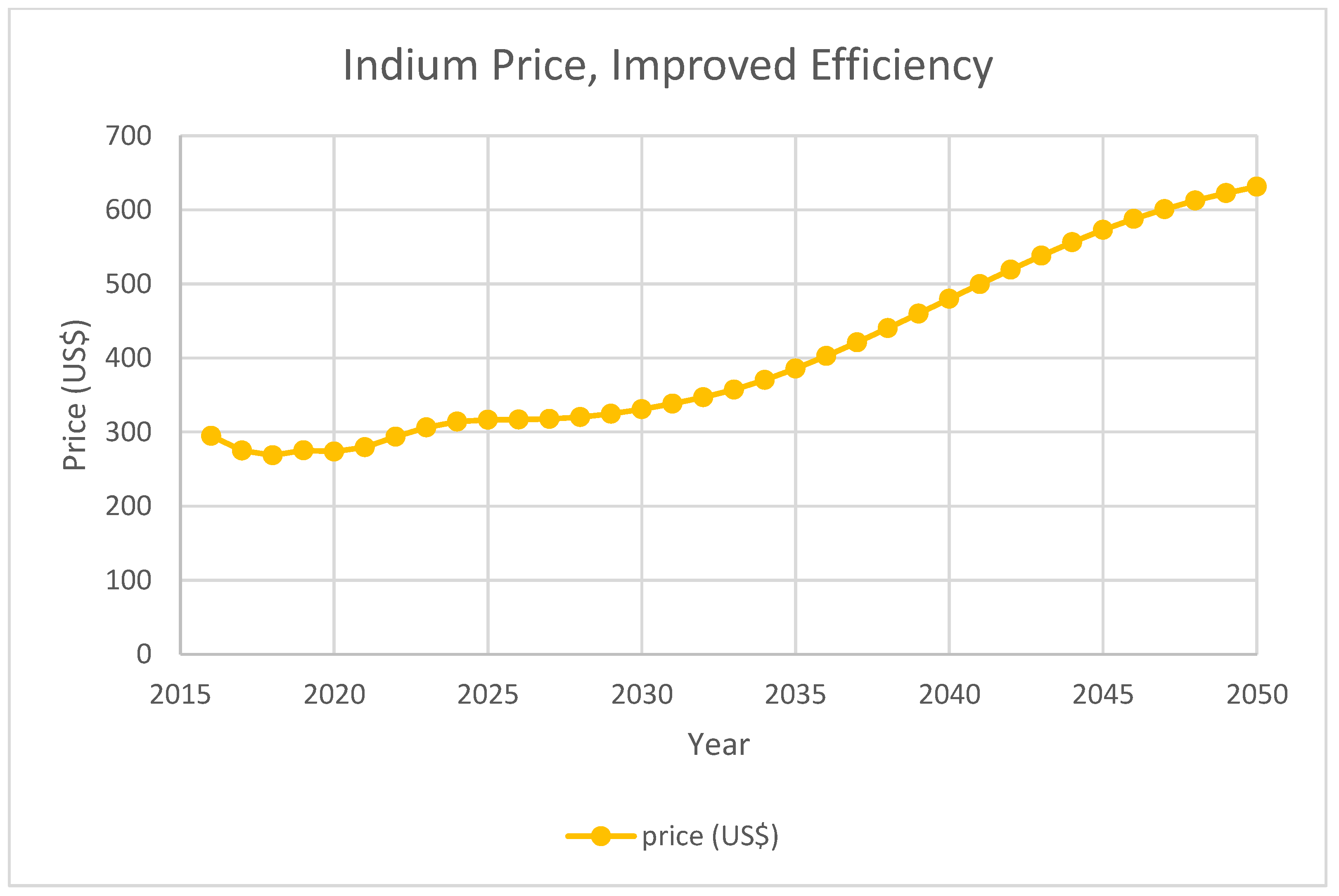
Indium price, improved indium efficiency.

Figure 18.
Supply–demand balance, ITO phase out.

Figure 19.
Primary indium supply vs. total demands.

Table 1.
ITO Loop Table.
| Cycle | 1 | 2 | 3 | 4 | 5 | 6 | 7 | 8 | 9 | 10 | 11 | 12 | 13 | 14 | 15 | Total |
|---|---|---|---|---|---|---|---|---|---|---|---|---|---|---|---|---|
| Units available (t) | 705.45 | 444.43 | 279.99 | 176.40 | 111.13 | 70.01 | 44.11 | 27.79 | 17.51 | 11.03 | 6.95 | 4.38 | 2.76 | 1.74 | 1.09 | 1904.76 |
| Units deposited (t) | 211.64 | 133.33 | 84.00 | 52.92 | 33.34 | 21.00 | 13.23 | 8.34 | 5.25 | 3.31 | 2.08 | 1.31 | 0.83 | 0.52 | 0.33 | 571.43 |
| Units for recycling (t) | 493.82 | 311.10 | 196.00 | 123.48 | 77.79 | 49.01 | 30.88 | 19.45 | 12.25 | 7.72 | 4.86 | 3.06 | 1.93 | 1.22 | 0.77 | 1333.33 |
| Units recycled (t) | 444.43 | 279.99 | 176.40 | 111.13 | 70.01 | 44.11 | 27.79 | 17.51 | 11.03 | 6.95 | 4.38 | 2.76 | 1.74 | 1.09 | 0.69 | 1200.00 |
| Units lost (t) | 49.38 | 31.11 | 19.60 | 12.35 | 7.78 | 4.90 | 3.09 | 1.95 | 1.23 | 0.77 | 0.49 | 0.31 | 0.19 | 0.12 | 0.08 | 133.33 |
Table 2.
CIGS Scenarios.
| Parameter | Pessimistic | Base | Optimistic |
|---|---|---|---|
| Layer thickness by 2020 (μm) | 1.2 | 1.0 | 0.8 |
| Layer thickness by 2050 (μm) | 0.8 | 0.8 | 0.8 |
| Annual production by 2050 (GW) | 17 | 54 | 105 |
| Efficiency by 2020 | 14% | 15.9% | 16.8% |
| Efficiency by 2050 | 22.9% | 22.9% | 22.9% |
Publisher’s Note: MDPI stays neutral with regard to jurisdictional claims in published maps and institutional affiliations. |
© 2021 by the authors. Licensee MDPI, Basel, Switzerland. This article is an open access article distributed under the terms and conditions of the Creative Commons Attribution (CC BY) license (https://creativecommons.org/licenses/by/4.0/).
Share and Cite
MDPI and ACS Style
Cao, J.; Choi, C.H.; Zhao, F. Agent-Based Modeling for By-Product Metal Supply—A Case Study on Indium. Sustainability 2021, 13, 7881. https://doi.org/10.3390/su13147881
AMA Style
Cao J, Choi CH, Zhao F. Agent-Based Modeling for By-Product Metal Supply—A Case Study on Indium. Sustainability. 2021; 13(14):7881. https://doi.org/10.3390/su13147881
Chicago/Turabian StyleCao, Jinjian, Chul Hun Choi, and Fu Zhao. 2021. "Agent-Based Modeling for By-Product Metal Supply—A Case Study on Indium" Sustainability 13, no. 14: 7881. https://doi.org/10.3390/su13147881
Note that from the first issue of 2016, this journal uses article numbers instead of page numbers. See further details here.