
Intelligent Backpropagation Networks with Bayesian Regularization for Mathematical Models of Environmental Economic Systems

 ,
,  ,
,
Abstract
:1. Introduction
- A novel application of AI-based intelligent backpropagation networks via Bayesian regularization for a nonlinear environmental economic system is presented effectively.
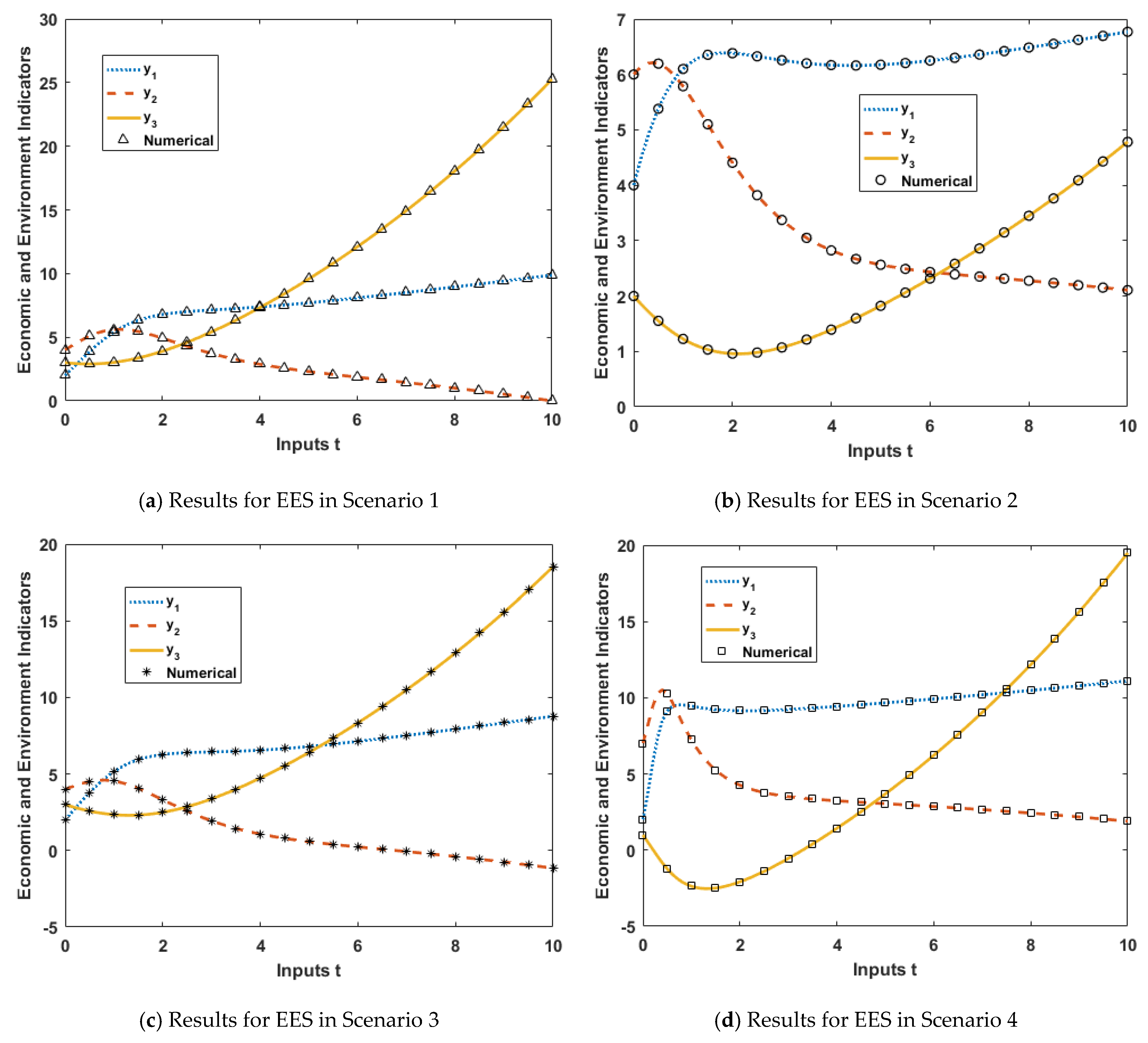
- The reference datasets for IBNs-BR for variants of a nonlinear environmental economic system are accurately assembled by implementation of the Adams numerical solver for different scenarios and are used as targets to find the approximate solutions.
- The governing mathematical relations of the nonlinear environmental economic system in the form of different differential models representing the fundamental compartments or indicators are viably solved with reasonable precision by the proposed IBNs-BR.
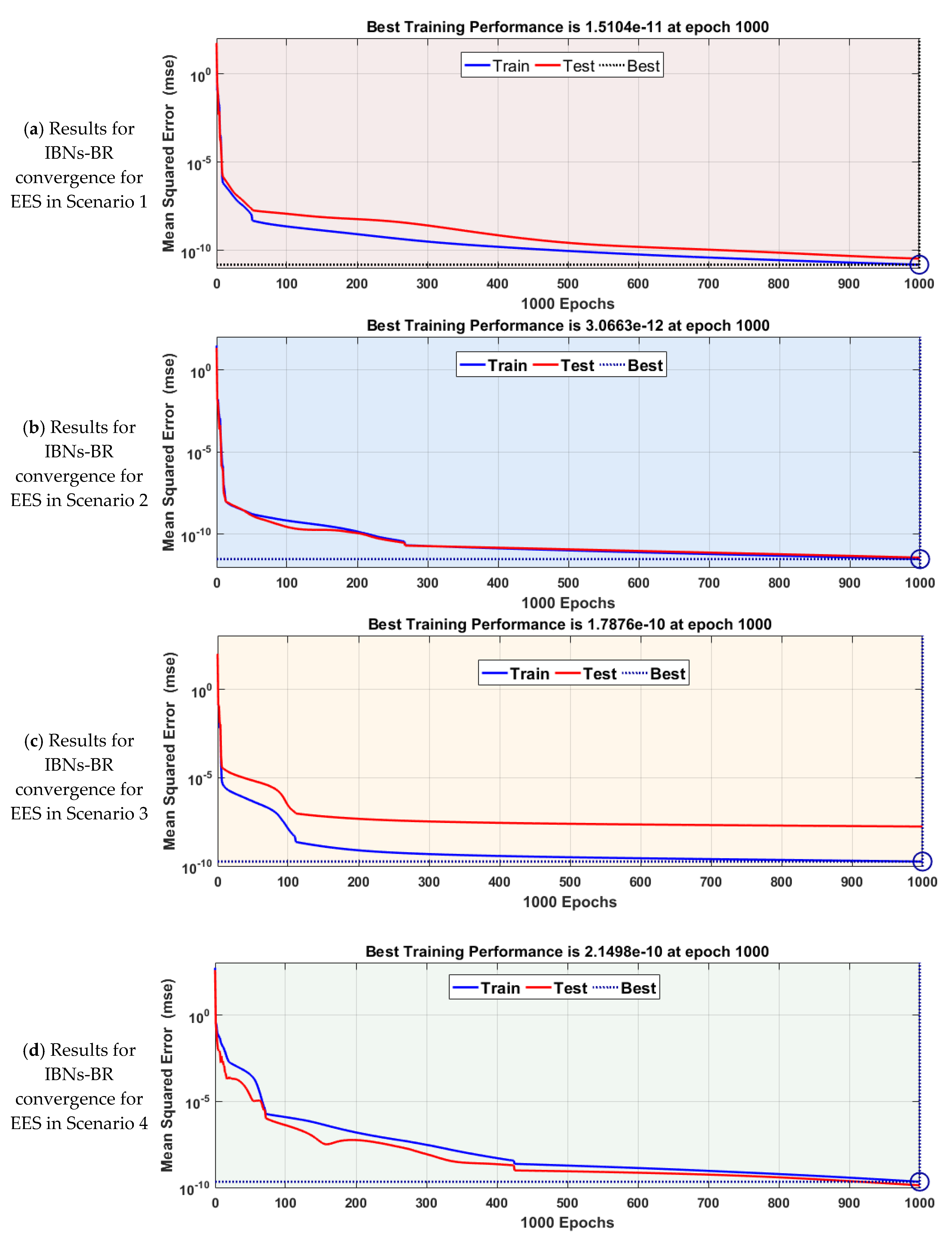
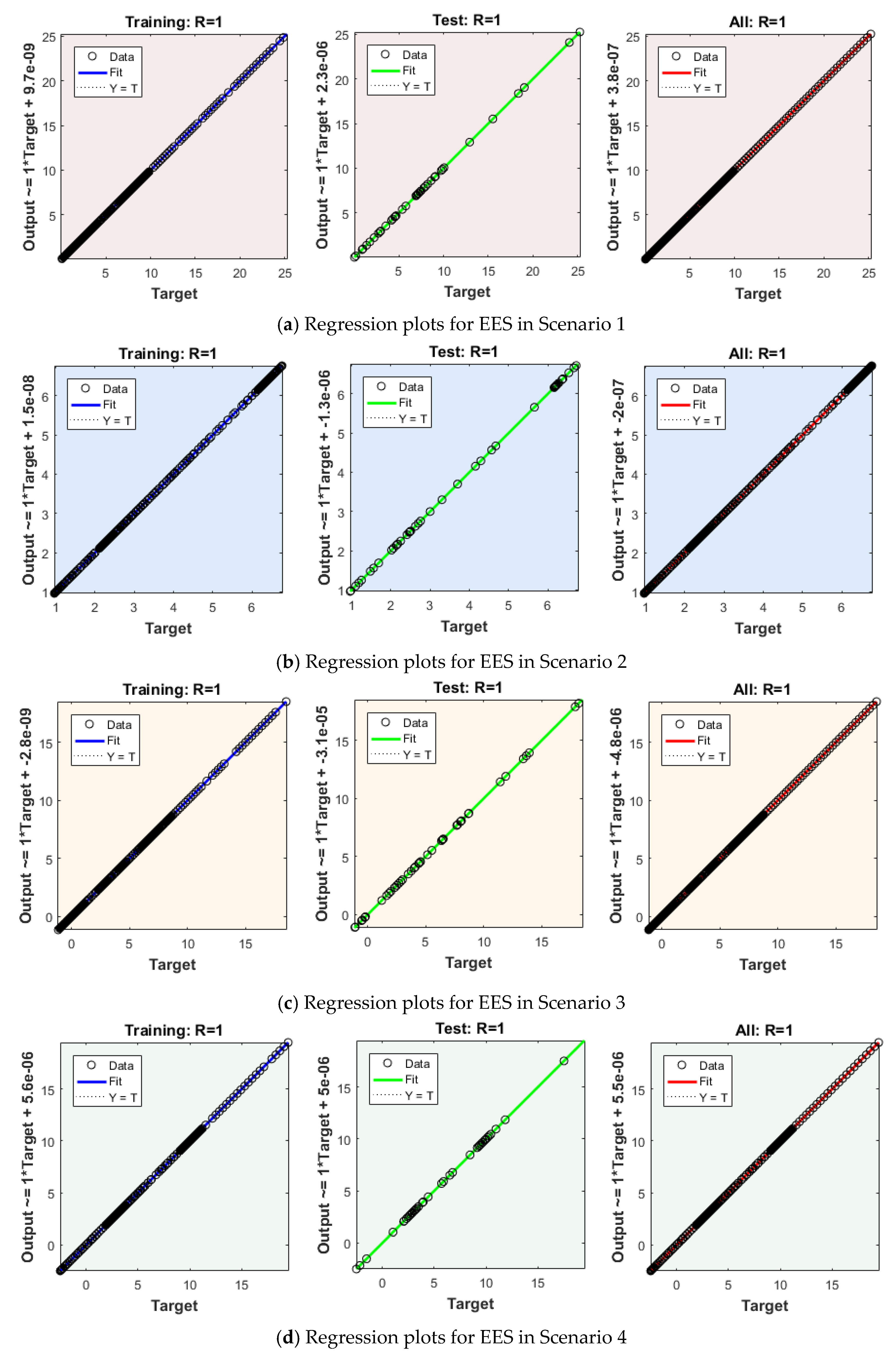
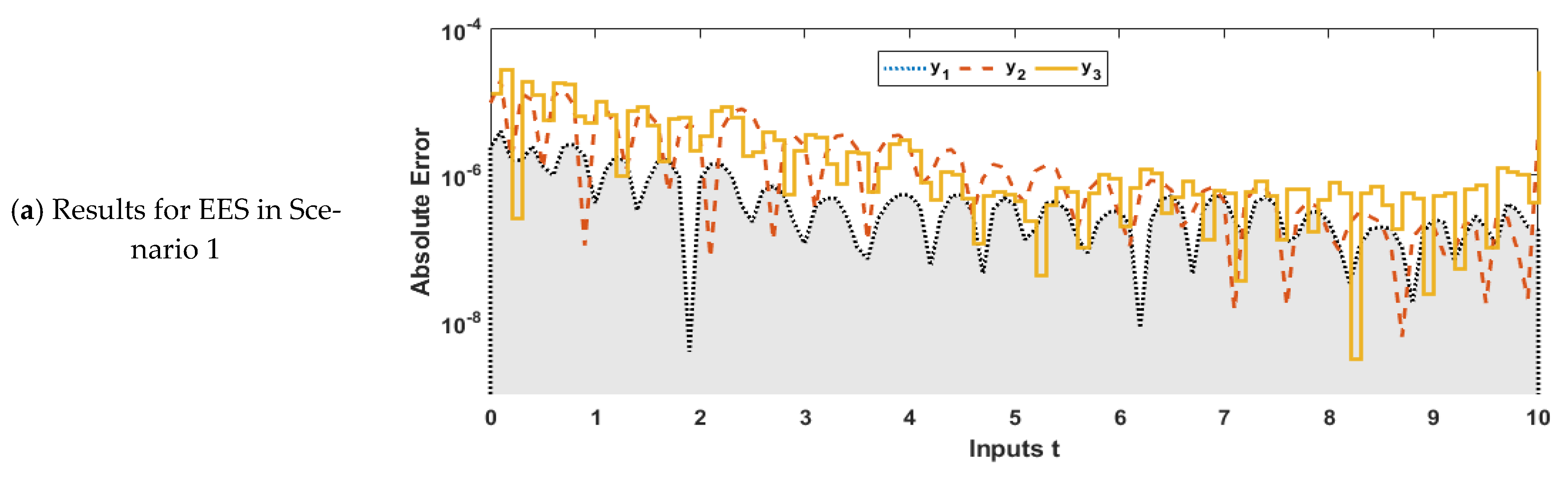
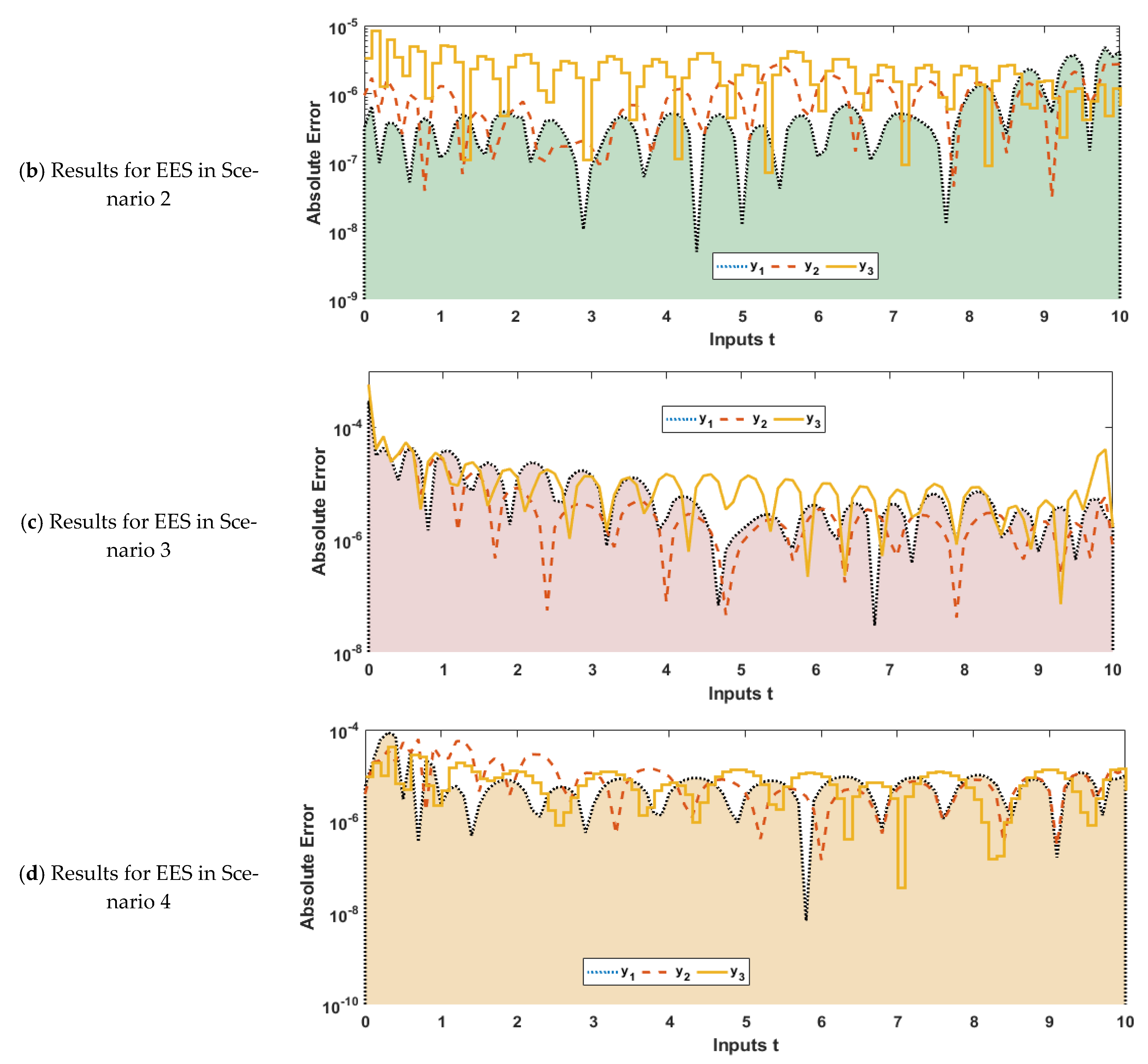
- The comparative studies based on convergence curves on the mean square error, error histogram analysis, and regression index are used to verify further the correctness of the IBNs-BR for each EES scenario.
2. Mathematical Representations
3. Solution Methodology
3.1. Adams Method
3.2. Intelligent Backpropagation Networks of Bayesian-Regularization
4. Results with Discussion
4.1. Dataset Formulation
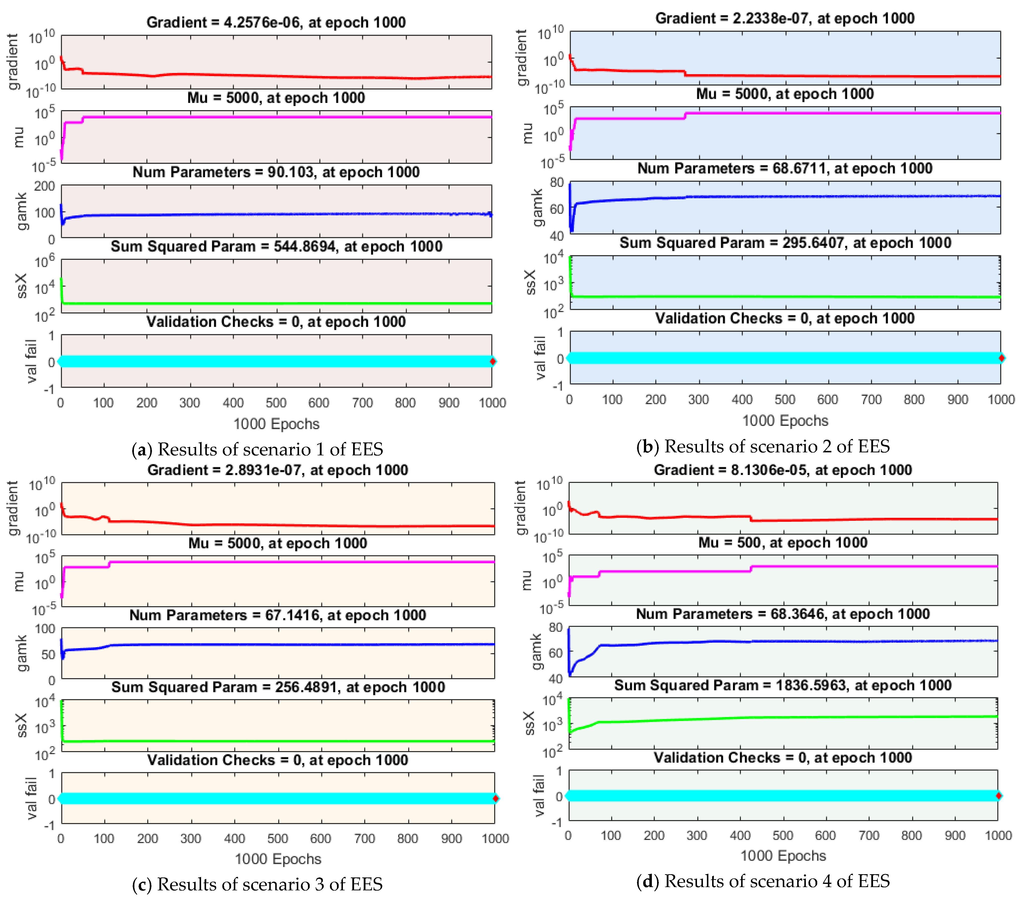
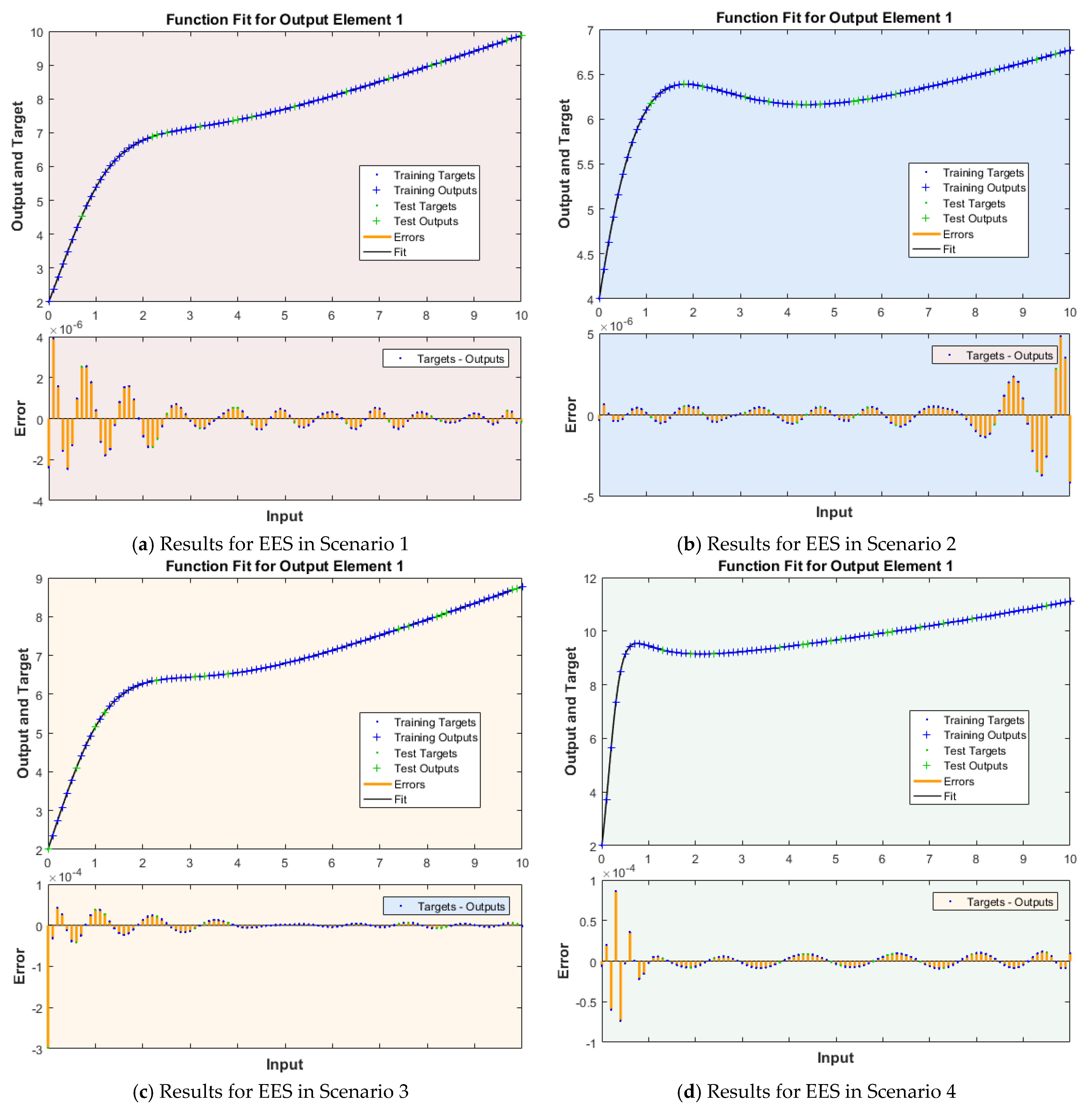
4.2. Implementation of IBNs-BR to EESs
4.3. Dynamical Analysis of EESs
5. Conclusions
- The purpose of this study was the exploration of the artificial intelligence-based computing paradigm for the numerical treatment of mathematical models representing the environmental economic systems using the competency of intelligent backpropagation networks of Bayesian regularization.
- The governing relations of the system model were presented in the form of differential models to portray the dynamics of fundamental compartments or indicators for economic and environmental parameters.
- The reference datasets of EESs were assembled by the Adams numerical solver for different scenarios and were used effectively as inputs and targets of IBNs-BR to predict the approximate solutions for each scenario.
- The comparative studies based on convergence curves on the mean square error and absolute deviation from the reference results consistently verified the correctness of IBNs-BR for solving EESs with an accuracy of the order 10−5 to 10−8.
- The endorsement of results was further validated through performance evaluation by means of error histogram analyses and the regression index for each EES scenario.
- Besides the advantage of consistent precision, stability, and robustness, the limitation of IBNs-BR depended mainly on the availability of the quality dataset for nonlinear systems, which is normally restricted for particular tasks and originations.
Author Contributions
Funding
Institutional Review Board Statement
Informed Consent Statement
Data Availability Statement
Conflicts of Interest
Appendix A. The Mathematical Formulation of the Adams Method Is Provided Here
Appendix B. Outcomes of the Adams Methods for Creation of Dataset for IBNs-BR

| Inputs | Economic Environment Indicators | ||
|---|---|---|---|
| t | y1(t) | y2(t) | y3(t) |
| 0 | 2 | 4 | 3 |
| 0.5 | 3.84987346535515 | 5.08244212918718 | 2.89983206145214 |
| 1.0 | 5.38531659314338 | 5.60035696874615 | 3.02244388419774 |
| 1.5 | 6.31817116386359 | 5.45256756062941 | 3.36661141796232 |
| 2.0 | 6.78228733954457 | 4.92388205874105 | 3.90153672089335 |
| 2.5 | 7.00449663338051 | 4.30075644696836 | 4.59090339781144 |
| 3.0 | 7.13623098005342 | 3.73058017059468 | 5.40443376949056 |
| 3.5 | 7.25183335675313 | 3.25771668447669 | 6.32030055915814 |
| 4.0 | 7.38077652717235 | 2.87767240448708 | 7.32412130274461 |
| 4.5 | 7.53094834169699 | 2.56932561549838 | 8.40715686297488 |
| 5.0 | 7.70123930149309 | 2.30972437108622 | 9.56461936718528 |
| 5.5 | 7.88768461971776 | 2.07962841891784 | 10.7943453899990 |
| 6.0 | 8.08617911929294 | 1.86475006148766 | 12.0958525223690 |
| 6.5 | 8.29344995816018 | 1.65522848140345 | 13.4697126068641 |
| 7.0 | 8.50721003291470 | 1.44456800915997 | 14.9171555129752 |
| 7.5 | 8.72599101627560 | 1.22859562054423 | 16.4398277156209 |
| 8.0 | 8.94890545811000 | 1.00463900609771 | 18.0396486908658 |
| 8.5 | 9.17544072696511 | 0.770951089310535 | 19.7187265507377 |
| 9.0 | 9.40531139975185 | 0.526336950522214 | 21.4793085598252 |
| 9.5 | 9.63836456840631 | 0.269924665643338 | 23.3237522313186 |
| 10.0 | 9.87452295609776 | 0.00102870600650036 | 25.2545082708319 |
| Inputs | Economic Environmental Indicators | ||
|---|---|---|---|
| t | y1(t) | y2(t) | y3(t) |
| 0 | 4 | 6 | 2 |
| 0.5 | 5.38100474030686 | 6.19554526232834 | 1.55111733320595 |
| 1.0 | 6.09927738409611 | 5.78633303573584 | 1.22577522357539 |
| 1.5 | 6.35548747400663 | 5.10069533413258 | 1.03331636004833 |
| 2.0 | 6.38365001669932 | 4.40540907962059 | 0.959395280990677 |
| 2.5 | 6.32741059555454 | 3.82051677909423 | 0.980021495694433 |
| 3.0 | 6.25670325749930 | 3.37310181214434 | 1.07134703343056 |
| 3.5 | 6.20078445218686 | 3.04961767687740 | 1.21373076020701 |
| 4.0 | 6.16905449643891 | 2.82392687172957 | 1.39254542281714 |
| 4.5 | 6.16183411641528 | 2.66950845315801 | 1.59762820134015 |
| 5.0 | 6.17572236173912 | 2.56393448235614 | 1.82233095710680 |
| 5.5 | 6.20625079853538 | 2.48993218909104 | 2.06257614455027 |
| 6.0 | 6.24915773972639 | 2.43503538904165 | 2.31606448168829 |
| 6.5 | 6.30092288055574 | 2.39072629889620 | 2.58166694972839 |
| 7.0 | 6.35890001042641 | 2.35148084367527 | 2.85898768612483 |
| 7.5 | 6.42124445300171 | 2.31390273648284 | 3.14806654367728 |
| 8.0 | 6.48675501340949 | 2.27602030458287 | 3.44918746382301 |
| 8.5 | 6.55470105666067 | 2.23676036819480 | 3.76276202864773 |
| 9.0 | 6.62467063891569 | 2.19558095066128 | 4.08926323486825 |
| 9.5 | 6.69645295396079 | 2.15223108486534 | 4.42919091212818 |
| 10.0 | 6.76995546919117 | 2.10660368730861 | 4.78305573981986 |
| Inputs. | Economic Environment Indicators | ||
|---|---|---|---|
| T | y1(t) | y2(t) | y3(t) |
| 0 | 2 | 4 | 3 |
| 0.5 | 3.77895369496549 | 4.50702615902379 | 2.57986824244645 |
| 1.0 | 5.15606353978099 | 4.54004425328471 | 2.34284450318794 |
| 1.5 | 5.93261912711357 | 4.05208819440336 | 2.31546105246105 |
| 2.0 | 6.27163900644184 | 3.31411029940714 | 2.49639713634012 |
| 2.5 | 6.39293747877504 | 2.57125227854606 | 2.86058165484202 |
| 3.0 | 6.44010758236978 | 1.93983291656762 | 3.37456519454619 |
| 3.5 | 6.48482877747975 | 1.44592884640699 | 4.00737246907302 |
| 4.0 | 6.55602144687651 | 1.07367395867702 | 4.73486421256424 |
| 4.5 | 6.66072938991790 | 0.793625447173174 | 5.54025511333904 |
| 5.0 | 6.79599374517557 | 0.576092093208258 | 6.41301055044085 |
| 5.5 | 6.95528465953494 | 0.396434840330269 | 7.34730733724330 |
| 6.0 | 7.13183052675037 | 0.236411861902662 | 8.34058681384511 |
| 6.5 | 7.32009801847897 | 0.0836561075986805 | 9.39240075126678 |
| 7.0 | 7.51618092406137 | −0.0695999811947876 | 10.5035824842229 |
| 7.5 | 7.71762412121082 | −0.227918622868782 | 11.6757031596123 |
| 8.0 | 7.92304264364204 | −0.393841773143552 | 12.9107442606998 |
| 8.5 | 8.13174176660711 | −0.568754881311778 | 14.2109166509352 |
| 9.0 | 8.34342528591773 | −0.753444025495404 | 15.5785699425160 |
| 9.5 | 8.55800463888684 | −0.948419108140589 | 17.0161524299301 |
| 10.0 | 8.77548867529859 | −1.15408310298745 | 18.5261967960712 |
| Inputs | Economic Environment Indicators | ||
|---|---|---|---|
| T | y1(t) | y2(t) | y3(t) |
| 0 | 2 | 7 | 1 |
| 0.5 | 9.13011744363290 | 10.2815684832990 | −1.22670568611237 |
| 1.0 | 9.45242179179267 | 7.23680780213549 | −2.36857214849340 |
| 1.5 | 9.22579404439015 | 5.25387957522542 | −2.49057226245891 |
| 2.0 | 9.14675405565877 | 4.26856757726780 | −2.07804071224031 |
| 2.5 | 9.16482726545373 | 3.77685508340256 | −1.38871862767779 |
| 3.0 | 9.23310909120640 | 3.51408824999788 | −0.542928109057926 |
| 3.5 | 9.32676271704346 | 3.35431273982965 | 0.405194804976283 |
| 4.0 | 9.43394815294133 | 3.23918943201718 | 1.43229103663283 |
| 4.5 | 9.54927152237131 | 3.14192356772089 | 2.52916646815619 |
| 5.0 | 9.67032894046072 | 3.05016712301859 | 3.69315485166567 |
| 5.5 | 9.79606431199662 | 2.95814742297101 | 4.92463297490176 |
| 6.0 | 9.92602277894565 | 2.86308318515682 | 6.22543190531976 |
| 6.5 | 10.0600172804611 | 2.76355602213811 | 7.59811147878160 |
| 7.0 | 10.1979802045286 | 2.65876881759113 | 9.04562878157438 |
| 7.5 | 10.3398972698181 | 2.54820591356171 | 10.5711866022534 |
| 8.0 | 10.4857783793664 | 2.43147767608113 | 12.1781652574761 |
| 8.5 | 10.6356441136913 | 2.30824774138989 | 13.8700926865631 |
| 9.0 | 10.7895202104004 | 2.17819978311887 | 15.6506325243711 |
| 9.5 | 10.9474347210994 | 2.04102137937621 | 17.5235803589099 |
| 10.0 | 11.1094171776640 | 1.89639672694744 | 19.4928646374896 |
References
- Verma, M.; Verma, A.K.; Misra, A.K. Mathematical modeling and optimal control of carbon dioxide emissions from energy sector. Environ. Dev. Sustain. 2021, 1–26. [Google Scholar] [CrossRef]
- Bherwani, H.; Anjum, S.; Gupta, A.; Singh, A.; Kumar, R. Establishing influence of morphological aspects on microclimatic conditions through GIS-assisted mathematical modeling and field observations. Environ. Dev. Sustain. 2021. [Google Scholar] [CrossRef]
- Nasrollahi, Z.; Hashemi, M.S.; Bameri, S.; Taghvaee, V.M. Environmental pollution, economic growth, population, industrialization, and technology in weak and strong sustainability: Using STIRPAT model. Environ. Dev. Sustain. 2020, 22, 1105–1122. [Google Scholar] [CrossRef]
- Montoya, O.Q.; Niño-Ruiz, E.D.; Pinel, N. On the mathematical modelling and data assimilation for air pollution assessment in the Tropical Andes. Environ. Sci. Pollut. Res. 2020, 27, 35993–36012. [Google Scholar] [CrossRef]
- El Aferni, A.; Guettari, M.; Tajouri, T. Mathematical model of Boltzmann’s sigmoidal equation applicable to the spreading of the coronavirus (Covid-19) waves. Environ. Sci. Pollut. Res. 2020, 1–9. [Google Scholar] [CrossRef]
- Hu, Y.; Jiang, H.; Zhong, Z. Impact of green credit on industrial structure in China: Theoretical mechanism and empirical analysis. Environ. Sci. Pollut. Res. 2020, 27, 10506–10519. [Google Scholar] [CrossRef] [PubMed]
- Wu, Z.; Wu, W. Theoretical analysis of pollutant mixing zone considering lateral distribution of flow velocity and diffusion coefficient. Environ. Sci. Pollut. Res. 2018, 26, 30675–30683. [Google Scholar] [CrossRef] [PubMed]
- Campos, C.F.; Cunha, M.C.; Santos, V.S.V.; de Campos Júnior, E.O.; Bonetti, A.M.; Pereira, B.B. Analysis of genotoxic effects on plants exposed to high traffic volume in urban crossing intersections. Chemosphere 2020, 259, 127511. [Google Scholar] [CrossRef] [PubMed]
- Taylor, K.H. Resuscitating (and Refusing) Cartesian representations of daily life: When mobile and grid epistemologies of the city meet. Cogn. Instr. 2020, 38, 407–426. [Google Scholar] [CrossRef]
- Chakraborty, A.; Maity, S.; Jain, S.; Mondal, S.P.; Alam, S. Hexagonal fuzzy number and its distinctive representation, ranking, defuzzification technique and application in production inventory management problem. Granul. Comput. 2021, 6, 507–521. [Google Scholar] [CrossRef]
- Reyniers, D.J. Supplier-customer interaction in quality control. Ann. Oper. Res. 1992, 34, 307–330. [Google Scholar] [CrossRef]
- Oliinyk, A.; Feshanych, L. The use of the apparatus of ordinary differential equations in simulation of economic and environmental systems. In Proceedings of the International Scientific and Technical Conference Information Technologies in Metallurgy and Machine Building; Ministry of Education and Science of Ukraine The National Metallurgical Academy of Ukraine, Dnipro, Ukraine, 17–19 March 2020; pp. 216–220. [Google Scholar] [CrossRef]
- Di Vaio, A.; Palladino, R.; Hassan, R.; Escobar, O. Artificial intelligence and business models in the sustainable development goals perspective: A systematic literature review. J. Bus. Res. 2020, 121, 283–314. [Google Scholar] [CrossRef]
- Zhao, L.; Dai, T.; Qiao, Z.; Sun, P.; Hao, J.; Yang, Y. Application of artificial intelligence to wastewater treatment: A bibliometric analysis and systematic review of technology, economy, management, and wastewater reuse. Process. Saf. Environ. Prot. 2020, 133, 169–182. [Google Scholar] [CrossRef]
- Di Vaio, A.; Boccia, F.; Landriani, L.; Palladino, R. Artificial intelligence in the agri-food system: Rethinking sustainable business models in the COVID-19 scenario. Sustainability 2020, 12, 4851. [Google Scholar] [CrossRef]
- Gregurec, I.; Tomičić Furjan, M.; Tomičić-Pupek, K. The impact of COVID-19 on sustainable business models in SMEs. Sustainability 2021, 13, 1098. [Google Scholar] [CrossRef]
- Kang, J.; Lee, H.J.; Jeong, S.H.; Lee, H.S.; Oh, K.J. Developing a Forecasting Model for Real Estate Auction Prices Using Artificial Intelligence. Sustainability 2020, 12, 2899. [Google Scholar] [CrossRef] [Green Version]
- Kachba, Y.; Chiroli, D.M.D.G.; Belotti, J.T.; Alves, T.A.; Tadano, Y.D.S.; Siqueira, H. Artificial Neural Networks to Estimate the Influence of Vehicular Emission Variables on Morbidity and Mortality in the Largest Metropolis in South America. Sustainability 2020, 12, 2621. [Google Scholar] [CrossRef] [Green Version]
- Ali, W.; Khan, W.U.; Raja, M.A.Z.; He, Y.; Li, Y. Design of Nonlinear Autoregressive Exogenous Model Based Intelligence Computing for Efficient State Estimation of Underwater Passive Target. Entropy 2021, 23, 550. [Google Scholar] [CrossRef]
- Sabir, Z.; Raja, M.A.Z.; Guirao, J.L.; Shoaib, M. A novel design of fractional Meyer wavelet neural networks with application to the nonlinear singular fractional Lane-Emden systems. Alex. Eng. J. 2021, 60, 2641–2659. [Google Scholar] [CrossRef]
- Sabir, Z.; Raja, M.A.Z.; Baleanu, D. Fractional Mayer Neuro-swarm heuristic solver for multi-fractional Order doubly singular model based on Lane-Emden equation. Fractals 2021, 29, 2140017. [Google Scholar] [CrossRef]
- Sabir, Z.; Raja, M.A.Z.; Umar, M.; Shoaib, M. Design of neuro-swarming-based heuristics to solve the third-order nonlinear multi-singular Emden–Fowler equation. Eur. Phys. J. Plus 2020, 135, 410. [Google Scholar] [CrossRef]
- Raja, M.A.Z.; Mehmood, J.; Sabir, Z.; Nasab, A.K.; Manzar, M.A. Numerical solution of doubly singular nonlinear systems using neural networks-based integrated intelligent computing. Neural Comput. Appl. 2019, 31, 793–812. [Google Scholar] [CrossRef]
- Sabir, Z.; Raja, M.A.Z.; Shoaib, M.; Aguilar, J.G. FMNEICS: Fractional Meyer neuro-evolution-based intelligent computing solver for doubly singular multi-fractional order Lane–Emden system. Comput. Appl. Math. 2020, 39, 1–18. [Google Scholar] [CrossRef]
- Raja, M.A.Z.; Shah, F.H.; Alaidarous, E.S.; Syam, M.I. Design of bio-inspired heuristic technique integrated with interior-point algorithm to analyze the dynamics of heartbeat model. Appl. Soft Comput. 2017, 52, 605–629. [Google Scholar] [CrossRef]
- Raja, M.A.Z.; Shah, F.H.; Syam, M.I. Intelligent computing approach to solve the nonlinear Van der Pol system for heartbeat model. Neural Comput. Appl. 2017, 30, 3651–3675. [Google Scholar] [CrossRef]
- Umar, M.; Sabir, Z.; Raja, M.A.Z.; Amin, F.; Saeed, T.; Guerrero-Sanchez, Y. Integrated neuro-swarm heuristic with interior-point for nonlinear SITR model for dynamics of novel COVID-19. Alex. Eng. J. 2021, 60, 2811–2824. [Google Scholar] [CrossRef]
- Umar, M.; Sabir, Z.; Raja, M.A.Z.; Shoaib, M.; Gupta, M.; Sánchez, Y.G. A Stochastic Intelligent Computing with Neuro-Evolution Heuristics for Nonlinear SITR System of Novel COVID-19 Dynamics. Symmetry 2020, 12, 1628. [Google Scholar] [CrossRef]
- Umar, M.; Raja, M.A.Z.; Sabir, Z.; Alwabli, A.S.; Shoaib, M. A stochastic computational intelligent solver for numerical treatment of mosquito dispersal model in a heterogeneous environment. Eur. Phys. J. Plus 2020, 135, 1–23. [Google Scholar] [CrossRef]
- Guo, Q.; He, Z. Prediction of the confirmed cases and deaths of global COVID-19 using artificial intelligence. Environ. Sci. Pollut. Res. 2021, 28, 11672–11682. [Google Scholar] [CrossRef]
- Umar, M.; Sabir, Z.; Raja, M.A.Z. Intelligent computing for numerical treatment of nonlinear prey–predator models. Appl. Soft Comput. 2019, 80, 506–524. [Google Scholar] [CrossRef]
- Raja, M.A.Z.; Malik, M.F.; Chang, C.L.; Shoaib, M.; Shu, C.M. Design of backpropagation networks for bioconvection model in transverse transportation of rheological fluid involving Lorentz force interaction and gyrotactic microorganisms. J. Taiwan Inst. Chem. Eng. 2021, 121, 276–291. [Google Scholar] [CrossRef]
- Ilyas, H.; Ahmad, I.; Raja, M.A.Z.; Tahir, M.B.; Shoaib, M. Intelligent networks for crosswise stream nanofluidic model with Cu–H2O over porous stretching medium. Int. J. Hydrog. Energy 2021, 46, 15322–15336. [Google Scholar] [CrossRef]
- Umar, M.; Sabir, Z.; Raja, M.A.Z.; Sánchez, Y.G. A stochastic numerical computing heuristic of SIR nonlinear model based on dengue fever. Results Phys. 2020, 19, 103585. [Google Scholar] [CrossRef]
- Aljohani, J.L.; Alaidarous, E.S.; Raja, M.A.Z.; Shoaib, M.; Alhothuali, M.S. Intelligent computing through neural networks for numerical treatment of non-Newtonian wire coating analysis model. Sci. Rep. 2021, 11, 1–32. [Google Scholar]
- Ara, A.; Khan, N.A.; Razzaq, O.A.; Hameed, T.; Raja, M.A.Z. Wavelets optimization method for evaluation of fractional partial differential equations: An application to financial modelling. Adv. Differ. Equ. 2018, 2018, 8. [Google Scholar] [CrossRef]
- Bukhari, A.H.; Raja, M.A.Z.; Sulaiman, M.; Islam, S.; Shoaib, M.; Kumam, P. Fractional neuro-sequential ARFIMA-LSTM for financial market forecasting. IEEE Access 2020, 8, 71326–71338. [Google Scholar] [CrossRef]
- Khan, B.S.; Raja, M.A.Z.; Qamar, A.; Chaudhary, N.I. Design of moth flame optimization heuristics for integrated power plant system containing stochastic wind. Appl. Soft Comput. 2021, 104, 107193. [Google Scholar] [CrossRef]
- Khan, I.; Raja, M.A.Z.; Shoaib, M.; Kumam, P.; Alrabaiah, H.; Shah, Z.; Islam, S. Design of Neural Network with Levenberg-Marquardt and Bayesian Regularization Backpropagation for Solving Pantograph Delay Differential Equations. IEEE Access 2020, 8, 137918–137933. [Google Scholar] [CrossRef]
- Wali, A.S.; Tyagi, A. Comparative Study of Advance Smart Strain Approximation Method Using Levenberg-Marquardt and Bayesian Regularization Backpropagation Algorithm. Mater. Today Proc. 2020, 21, 1380–1395. [Google Scholar] [CrossRef]
- Zhao, H.; Zhang, C. An online-learning-based evolutionary many-objective algorithm. Inf. Sci. 2020, 509, 1–21. [Google Scholar] [CrossRef]
- Ilyas, H.; Raja, M.A.Z.; Ahmad, I.; Shoaib, M. A novel design of Gaussian Wavelet Neural Networks for nonlinear Falkner-Skan systems in fluid dynamics. Chin. J. Phys. 2021, 72, 386–402. [Google Scholar] [CrossRef]
- Dulebenets, M.A. A novel memetic algorithm with a deterministic parameter control for efficient berth scheduling at marine container terminals. Marit. Bus. Rev. 2017, 2, 302–330. [Google Scholar] [CrossRef] [Green Version]
- Shoaib, M.; Raja, M.A.Z.; Khan, M.A.R.; Farhat, I.; Awan, S.E. Neuro-Computing Networks for Entropy Generation under the Influence of MHD and Thermal Radiation. Surf. Interfaces 2021, 25, 101243. [Google Scholar] [CrossRef]
- Liu, Z.Z.; Wang, Y.; Huang, P.Q. AnD: A many-objective evolutionary algorithm with angle-based selection and shift-based density estimation. Inf. Sci. 2020, 509, 400–419. [Google Scholar] [CrossRef] [Green Version]
- Pasha, J.; Dulebenets, M.A.; Kavoosi, M.; Abioye, O.F.; Wang, H.; Guo, W. An Optimization Model and Solution Algorithms for the Vehicle Routing Problem with a “Factory-in-a-Box”. IEEE Access 2020, 8, 134743–134763. [Google Scholar] [CrossRef]
- Sabir, Z.; Sabir, Z.; Raja, M.A.Z.; Le, D.-N.; Aly, A.A. A neuro-swarming intelligent heuristic for second-order nonlinear Lane–Emden multi-pantograph delay differential system. Complex. Intell. Syst. 2021. [Google Scholar] [CrossRef]
- D’Angelo, G.; Pilla, R.; Tascini, C.; Rampone, S. A proposal for distinguishing between bacterial and viral meningitis using genetic programming and decision trees. Soft Comput. 2019, 23, 11775–11791. [Google Scholar] [CrossRef]
- Naz, S.; Raja, M.A.Z.; Mehmood, A.; Zameer, A.; Shoaib, M. Neuro-intelligent networks for Bouc–Wen hysteresis model for piezostage actuator. Eur. Phys. J. Plus 2021, 136, 1–20. [Google Scholar] [CrossRef]
- Panda, N.; Majhi, S.K. How effective is the salp swarm algorithm in data classification. In Computational Intelligence in Pattern Recognition; Springer: Singapore, 2020; pp. 579–588. [Google Scholar]
- Mehmood, A.; Shi, P.; Raja, M.A.Z.; Zameer, A.; Chaudhary, N.I. Design of backtracking search heuristics for parameter estimation of power signals. Neural Comput. Appl. 2021, 33, 1479–1496. [Google Scholar] [CrossRef]
- Awais, M.; Awan, S.E.; Raja, M.A.Z.; Shoaib, M. Effects of Gyro-Tactic organisms in bio-convective nano-material with heat immersion, stratification, and viscous dissipation. Arab. J. Sci. Eng. 2021, 46, 5907–5920. [Google Scholar] [CrossRef]
- Awan, S.E.; Raja, M.A.Z.; Gul, F.; Khan, Z.A.; Mehmood, A.; Shoaib, M. Numerical Computing Paradigm for Investigation of Micropolar Nanofluid Flow between Parallel Plates System with Impact of Electrical MHD and Hall Current. Arab. J. Sci. Eng. 2021, 46, 645–662. [Google Scholar] [CrossRef]
- Brodny, J.; Tutak, M. The analysis of similarities between the European Union countries in terms of the level and structure of the emissions of selected gases and air pollutants into the atmosphere. J. Clean. Prod. 2021, 279, 123641. [Google Scholar] [CrossRef]
- Tutak, M.; Brodny, J.; Bindzár, P. Assessing the Level of Energy and Climate Sustainability in the European Union Countries in the Context of the European Green Deal Strategy and Agenda 2030. Energies 2021, 14, 1767. [Google Scholar] [CrossRef]
- Tutak, M.; Brodny, J.; Szurgacz, D.; Sobik, L.; Zhironkin, S. The Impact of the Ventilation System on the Methane Release Hazard and Spontaneous Combustion of Coal in the Area of Exploitation—A Case Study. Energies 2020, 13, 4891. [Google Scholar] [CrossRef]
- Brodny, J.; Tutak, M. The Use of Artificial Neural Networks to Analyze Greenhouse Gas and Air Pollutant Emissions from the Mining and Quarrying Sector in the European Union. Energies 2020, 13, 1925. [Google Scholar] [CrossRef] [Green Version]
- Tutak, M.; Brodny, J.; Dobrowolska, M. Assessment of work conditions in a production enterprise—A case study. Sustainability 2020, 12, 5390. [Google Scholar] [CrossRef]
- Tutak, M. The influence of the permeability of the fractures zone around the heading on the concentration and distribution of methane. Sustainability 2020, 12, 16. [Google Scholar] [CrossRef] [Green Version]
- Nosratabadi, S.; Pinter, G.; Mosavi, A.; Semperger, S. Sustainable banking; Evaluation of the European business models. Sustainability 2020, 12, 2314. [Google Scholar] [CrossRef] [Green Version]
- Rjoub, H.; Odugbesan, J.A.; Adebayo, T.S.; Wong, W.K. Sustainability of the moderating role of financial development in the determinants of environmental degradation: Evidence from Turkey. Sustainability 2021, 13, 1844. [Google Scholar] [CrossRef]
- Nosratabadi, S.; Mosavi, A.; Shamshirband, S.; Kazimieras Zavadskas, E.; Rakotonirainy, A.; Chau, K.W. Sustainable business models: A review. Sustainability 2019, 11, 1663. [Google Scholar] [CrossRef] [Green Version]


| t | Scenario 1 | Scenario 2 | Scenario 3 | Scenario 4 | ||||||||
|---|---|---|---|---|---|---|---|---|---|---|---|---|
| y1(t) | y2(t) | y3(t) | y1(t) | y2(t) | y3(t) | y1(t) | y2(t) | y3(t) | y1(t) | y2(t) | y3(t) | |
| 0 | 2 | 4 | 3 | 4 | 6 | 2 | 2 | 4 | 3 | 9.130 | 10.281 | −1.226 |
| 1.0 | 5.385 | 5.600 | 3.022 | 6.099 | 5.786 | 1.225 | 5.156 | 4.540 | 2.342 | 9.452 | 7.236 | −2.368 |
| 2.0 | 6.782 | 4.923 | 3.901 | 6.3832 | 4.405 | 0.959 | 6.271 | 3.314 | 2.496 | 9.225 | 5.253 | −2.490 |
| 3.0 | 7.136 | 3.730 | 5.404 | 6.256 | 3.373 | 1.071 | 6.440 | 1.939 | 3.374 | 9.146 | 4.268 | −2.078 |
| 4.0 | 7.380 | 2.877 | 7.324 | 6.169 | 2.823 | 1.392 | 6.556 | 1.073 | 4.734 | 9.164 | 3.776 | −1.388 |
| 5.0 | 7.701 | 2.309 | 9.564 | 6.175 | 2.563 | 1.822 | 6.795 | 0.576 | 6.413 | 9.233 | 3.514 | −0.542 |
| 6.0 | 8.086 | 1.864 | 12.095 | 6.249 | 2.435 | 2.316 | 7.131 | 0.236 | 8.340 | 9.326 | 3.354 | 0.405 |
| 7.0 | 8.507 | 1.444 | 14.917 | 6.358 | 2.351 | 2.858 | 7.516 | −0.069 | 10.503 | 9.433 | 3.239 | 1.432 |
| 8.0 | 8.948 | 1.004 | 18.039 | 6.486 | 2.276 | 3.449 | 7.923 | −0.393 | 12.910 | 9.549 | 3.141 | 2.529 |
| 9.0 | 9.405 | 0.526 | 21.479 | 6.624 | 2.195 | 4.089 | 8.343 | −0.753 | 15.578 | 9.670 | 3.050 | 3.693 |
| 10.0 | 9.874 | 0.001 | 25.254 | 6.769 | 2.106 | 4.783 | 8.775 | −1.154 | 18.526 | 9.796 | 2.958 | 4.9246 |
Publisher’s Note: MDPI stays neutral with regard to jurisdictional claims in published maps and institutional affiliations. |
© 2021 by the authors. Licensee MDPI, Basel, Switzerland. This article is an open access article distributed under the terms and conditions of the Creative Commons Attribution (CC BY) license (https://creativecommons.org/licenses/by/4.0/).
Share and Cite
Kiani, A.K.; Khan, W.U.; Raja, M.A.Z.; He, Y.; Sabir, Z.; Shoaib, M. Intelligent Backpropagation Networks with Bayesian Regularization for Mathematical Models of Environmental Economic Systems. Sustainability 2021, 13, 9537. https://doi.org/10.3390/su13179537
Kiani AK, Khan WU, Raja MAZ, He Y, Sabir Z, Shoaib M. Intelligent Backpropagation Networks with Bayesian Regularization for Mathematical Models of Environmental Economic Systems. Sustainability. 2021; 13(17):9537. https://doi.org/10.3390/su13179537
Chicago/Turabian StyleKiani, Adiqa Kausar, Wasim Ullah Khan, Muhammad Asif Zahoor Raja, Yigang He, Zulqurnain Sabir, and Muhammad Shoaib. 2021. "Intelligent Backpropagation Networks with Bayesian Regularization for Mathematical Models of Environmental Economic Systems" Sustainability 13, no. 17: 9537. https://doi.org/10.3390/su13179537