Indoor Millimeter-Wave Propagation Prediction by Measurement and Ray Tracing Simulation at 38 GHz

Abstract

The Millimeter-Wave (mmW) technology is going to mitigate the global higher bandwidth carriers. It will dominate the future network system by the attractive advantages of the higher frequency band. Higher frequency offers a wider bandwidth spectrum. Therefore, its utilizations are rapidly increasing in the wireless communication system. In this paper, an indoor mmW propagation prediction is presented at 38 GHz based on measurements and the proposed Three-Dimensional (3-D) Ray Tracing (RT) simulation. Moreover, an additional simulation performed using 3-D Shooting Bouncing Ray (SBR) method is presented. Simulation using existing SBR and the proposed RT methods have been performed separately on a specific layout where the measurement campaign is conducted. The RT methods simulations results have been verified by comparing with actual measurement data. There is a significant agreement between the simulation and measurement with respect to path loss and received signal strength indication. The analysis result shows that the proposed RT method output has better agreement with measurement output when compared to the SBR method. According to the result of the propagation prediction analysis, it can be stated that the proposed method’s ray tracing is capable of predicting the mmW propagation based on a raw sketch of the real environment.

1. Introduction

The mmW frequency band is most promising for overcoming the gigabits per second barrier in the upcoming Wireless Communication System (WCS) [1]. With reference of global data growth in cellular communication predicted by CISCO, the data growth will be seven times higher by 2021 when compared with the data demand of 2016. The estimated cellular data growth will be 143 Exabyte per quarter by 2021 [2]. The mmW wave band is uniquely fit to serve the upcoming bandwidth hunger due to wider accessible bandwidth, frequency reutilization, and the minimized size of the base station and the mobile station components [3]. A single carrier frequency division multiple access extended was an excellent hopeful radio wave access technology for the fourth generation, the third generation partnership project and long term evolution, and the long-term evolution advanced networks cellular system [4,5]. Right now for the 5G application, we need to move toward the higher frequency like mmW. The application of this study covers a great research area such as the advent of the Internet of Things and the Fifth Generation (5G) network planning era where optimum WCS channels categorizations have a direct impact on the resource allocation process [6]. However, vast knowledge is needed on radio wave propagation to design mmW WCS. The frequencies band above 10 GHz not only considers the general propagation feathers like reflection, diffraction, and refraction but also needs to incorporate an environmental atmosphere effect such as rain, snow, storm, and the handover effect for mobility [7,8,9]. This study covers the indoor radio propagation, which is free from rain, snow, storm, and ignorable mobility.

The frequency 38 GHz is most suitable for the 5G networks frequency in WCS from the estimated mmW band [10,11,12]. To get the standard judgment of performance in WCS, a practical analysis of the propagation prediction for mmW is needed as a requirement for the cell deployment. The experimental way to evaluate the radio channels in a particular scenario is to measure the Received Signal Strength Indication (RSSI) and the Path Loss (PL) at multiple positions among the area by the deploying Receiver (Rx). To serve this persistence, an experimental measurement campaign has been performed on new wireless communication centers. The experimental environment is the basement floor of a two-story building in Universiti Teknologi Malaysia (UTM), in Johor Bahru Campus at Malaysia name as NWCC_P15a. The opportunity to run a measurement campaign is limited because a site-specific method is used in measurement, which makes the process time-consuming and costly. In this circumstance, RT simulation is robustly utilized for categorizing radio channel propagation for mmW. The RT is an essential tool for different smart technologies and WCS design [13]. It significantly reduces the use of time-consuming extensive costly measurement campaigns [14,15,16]. In the RT method, a ray is launched from the base station (TX) based on Uniform Theory of Diffraction (UTD) and Geometric Optics (GO). Furthermore, small-wavelength electromagnetic signal propagation is suitable for explaining the ray-optic estimate method, so RT simulation methods have been extensively used for the mmW in WCS [17]. Therefore, to replace a time-consuming and expensive measurement campaign, the RT simulation method can be utilized since it incorporated all the geometric principals accurately.

The dependency of scenarios, Ray Launching (RL) continual angular dimension, and environmental objects accurate modeling is the main challenge of RT simulation. Additionally, reflection, diffraction, and refraction features of RT needs to be implemented correctly. In this study, a proposed algorithm developed for 3-D RT is implemented in the simulator. Furthermore, the SBR method is also implemented in the RT simulator for comparison of simulation time, the number of rays launched, and the number of rays received by Rx with a proposed method. As per literature review, SBR is a widely used method for indoor mmW channels modeling [18]. However, most of the simulation-related articles are rarely found to have comprehensive information about the simulation environment. The simulation environment property is partially found in References [19,20,21]. However, simulation parameters like the highest number of reflection values and different obstacle penetration properties are not deeply analyzed when comparing with measurements.

The manuscript is organized as follows. The description of the measurement campaign is presented in the second section. The RT modeling is mentioned in section three. The validation of RT simulation is done by comparing with measurement data and is shown in section four. Lastly, the conclusion and future directions of this paper are stated in the last section.

2. Measurement Details

The measurement of the mmW propagation prediction in 5G networks at 38 GHz is carried out for capturing detailed information. This measurement campaign is conducted to estimate the Line of Sight (LoS) as well as Non-Line of Sight (NLoS) signals. The campaign is done in the NWCC_P15a building ground floor. The interior big rooms are partitioned by using approximately 5 cm thick glass and board. Additionally, some exterior door/windows are used and those are made with wood, plastic, and glass. One base station and 20 mobile stations are used in the measurement campaign. In the NWCC_P15a, mobile stations are placed in several areas to capture the LoS and NLoS signals within 1 to 22.7 m distances. NWCC_P15a height and width were 21 and 3 m. In the measurement campaign, the base station is placed in a fixed location of room 2 in the NWCC_P15a. The measurement is started from a 1-m distance mobile station from the base station. The RSSI and PL are captured in the Rx stationary at that point with respect to the position. Subsequently, the Rx changes location by moving 1 m apart from the TX. For every Rx point, the same process will be re-run until the measurement campaign finishes. An Anritsu MG369xC model signal generator is used to produce continues mmW, which is linked with a horn antenna. For the receiver, an MS2720T model omnidirectional antenna is used to receive frequency. The measurement used hardware configurations, which are given in

Table 1. Antenna configuration details.

SL.	Item	Properties
I	Gain (dB)	20
II	Frequency range (GHz)	26.5–40.0
III	Beamwidth (deg.)	18
IV	Waveguide	WR28
V	Material	Cu
VI	Output	A Type: FBP 320, C Type: 2.9 or 2.4 mm-F
VII	Size (mm) W × H × L	A Type: 40.5 × 32 × 70, C Type: 40.5 × 32 × 95
VIII	Net Weight (Kg)	A Type: 0.05 Around, C type 10 Around

.

In this measurement campaign, a horn antenna is used to transmit a signal at the base station and an omnidirectional antenna is used to receive a signal at the mobile station. For the measurement, some configurable parameters are actively incorporated, which are presented in

Table 2. Configurable measurement parameters.

SL.	Item	Values/Properties
I	Carrier frequency (GHz)	38
II	Transmit power (dBm)	25
III	TX horn antenna gain (dBi)	21.1
IV	Rx Omni antenna gain (dBi)	3
V	TX horn antenna height (meter)	2

.

The PL is a crucial factor in measuring WCS. PL is the large-scale fading calculation based on 38 GHz frequency depending on signal attenuation in a mobile station placed environment. WCS propagation characteristics are investigated based on empirical, stochastic PL and an empirical method [22,23]. Moreover, accurate PL increases the measurement accuracy in WCS [24,25]. Generally, PL is calculated in the measurement based on Equation (1).

$${P_{loss}}^{CI}\left(f,d\right)\left[dB\right]=P_{loss}\left(f,d_0\right)+10{\log }_{10}\left(d|d_0\right)+X_{\sigma }$$

(1)

In this scenario, $P_{loss}\left(f,d\right)$ is used to express the PL among all TX-Rx distance at the frequency 38 GHz. Additionally, $P_{loss}\left(f,d_0\right)$ is used to mean the PL for closing in the (CI) path. The symbol $d_0$ and $X_{\sigma }$ is used for the Zero Mean Gaussian Random Variable (ZMGRV) where standard deviation (SD) is symbolize by $X_{\sigma }$. The sensitivity (XPD) and Cross-Polarization (CP) has an additional effect on the CI PL model during the time of broadcast CP. It is described as the CI path within the XPD (CIX) PL that can be driven by Equation (2) [26].

$${P_{loss}}^{CIX}\left(f,d\right)\left[dB\right]=P_{loss}\left(f,d_0\right)+10n{\log }_{10} \left(d|d_0\right)+XPD+{X_{\sigma }}^{CIX}$$

(2)

The CP factor XPL can be driven by Equation (3).

$$XPD\left(f,d\right)\left[dB\right]=P_{loss\left(V-V\right)}-P_{loss\left(V-H\right)}$$

(3)

The term $P_{loss\left(V-V\right)}$ and $P_{loss\left(V-H\right)}$ are shown the co-polarization and CP PL, respectively. The XPD is identified using Equation (3), which is an average of cumulative XPL between the total path at 38 GHz frequency of f (see Equation (4)).

$$XPD\left(f\right)= \overline{XPL\left(f,d\right)}$$

(4)

The XPD value of Equation (4) is the reverse engineering of Equation (2) and the shadow fading is bring Equation (5).

$${X_{\sigma }}^{CIX}= {P_{loss}}^{CIX}\left(f,d\right)\left[dB\right]-P_{loss}\left(f,d_0\right)-10n{\log }_{10} \left(d|d_0\right)+XPD$$

(5)

To calculate the XPD feature, the study incorporated by a modified PL model name is the Frequency Attenuation (FA) PL model. The FA PL can be written by Equation (6).

$${P_{loss}}^{FA}\left(f,d\right)\left[dB\right]=P_{loss}\left(f_{ref},d_0\right)+10n_{ref}{\log }_{10} \left(d|d_0\right)+XF\left(f\right)+{X_{\sigma }}^{FA}$$

(6)

The term $P_{loss}\left(f_{ref},d_0\right)$ is indicated by PL at the CI path in the $d_0$ meter distance and $f_{ref}$ is the user for 38 GHz frequency. The model defined the $f_{ref}$ is the lowest frequency for the adjustment scenario. The term $n_{ref}$ is the PL exponent at $f_{ref }$ frequency, which is from the CI PL model with respect to vertical-to-vertical and antenna setup. The term $XF\left(f\right)$ express the FA factor, which mean the signal interfere because of reference frequency and ${X_{\sigma }}^{FA}$ is express shadow fading (SF) with an SD of σ.

3. Radio Wave Propagation Modeling by Ray-Tracing Simulation

3.1. SBR Ray Tracing Method

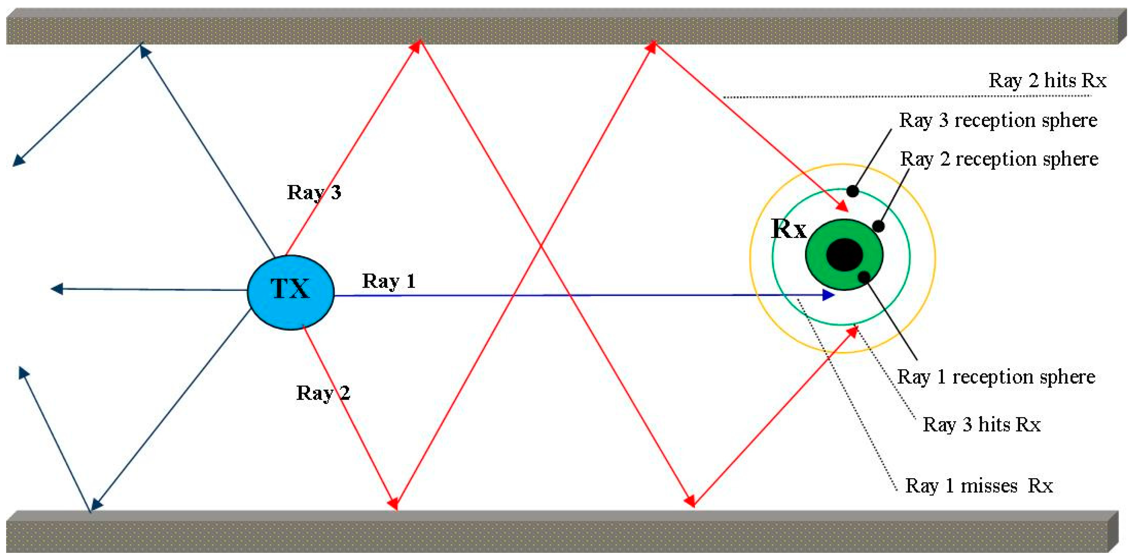
The SBR method is widely used in ray tracing to cover higher frequency radio propagation modeling. The basic SBR method is proposed by H. Ling to detect the “radar cross section of cavities” [27] and is enhanced to identify the statures of targeted objects [28]. Currently, SBR is the most renowned method for reflections and scattering modeling in WCS. From the base station, rays are shot in all the directions. As per ray characteristics, launched rays will be reflected from multiple objects before reaching the destination Rx. The Rx is detected based on the radius area sphere with respect to the ray path length and the regulation angle between launched rays. The SBR method is graphically presented in Figure 1 for the indoor scenario.

The calculation complexity and simulation time of the SBR method directly related to the number of objects in the environment and the RL angles regulations. Since the ray launched in all directions in the simulation area, the ray tracing zone gets wider for higher order of reflection and diffraction. For this wider range, launched rays increase the complexity of the SBR method to implement a huge computational recourse. Moreover, it is good for the crowd indoor environment, but is not suitable for the indoor environment by bearing less numbers of Rx as the number of rays launched are the same.

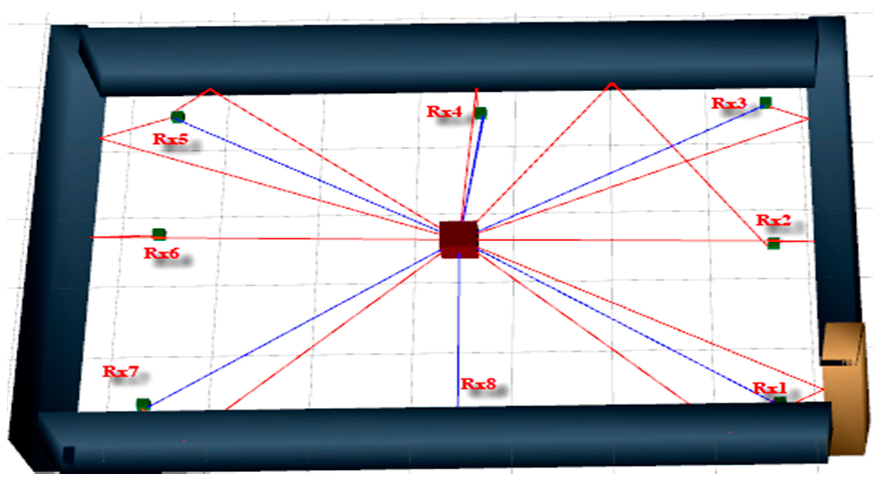
In Figure 2, RT has been performed within eight mobile stations and one base station considering both the LoS and NLoS signal using the SBR method.

3.2. Conventional RT Method Limitations

In a conventional RT method, rays are launched in all the possible directions with several angle resolutions without sensing the receiver locations. Therefore, in this circumstance, there is a need to run 3-D RT for every single ray, which is very much time consuming and costly. In the final stage, rays may successfully reach the mobile station sphere or rays may not collide with the receiver spheres. For processing, the high volume of rays, without any pre-assessment, occupied a huge computer resource and had a higher computational time. The fundamental disadvantage of the existing techniques is that the predefined probable zone concept is not incorporated for the receiver. Furthermore, it bounded to RL in all angles through the scenario from TX. For this type of mention, the limitation of the conventional method in simulation time, coverage, PL, RSSI, and RL is very hampering badly.

3.3. Proposed RT Model

In the proposed method, more rays were launched in the predefined zone. Moreover, to increase the accuracy, it does not allow us to permit it to launch rays in all the directions surrounded by the base station.

Proposed 3-D RT method works in several stages. Those are mentioned below.

• In phase I, scenario wise 3-D layout design considering the major object with respect to a mobile station and base stations.
• In phase II, RL from the base station and incorporate as reflection, refraction, and diffraction as per RT characteristics. Based on layout, used θ = π/60 for the RL angular regulation. This angle is variable. Therefore, a higher angle difference means fewer rays are needed to launch.
• In phase III, only some mathematical pre calculations have been performed to sort out the successive angle those rays successfully reached in the destinations.
• In phase IV, at least two onward additional directions are added to deliver more rays on the probable zone. The additional angle regulation depends on the scenario such as 0.25, 0.50, 0.75, or 1.0 from the determine angle.

            List<double> Probable_VerticalAngles = new List<double> ();
            if (Determine_VerticalAngles != NULL)
                 {
                     Probable_VerticalAngles.Add(Determine_VerticalAngles + π/240);
                     Probable_VerticalAngles.Add(Determine_VerticalAngles + π/120);
                 }
            

• In phase V, again determine the angle wise at least two backward additional directions and add more rays to deliver on the probable zone. The additional angle regulation depends on the scenario such as −0.25, −0.50, −0.75, or −1.0 forward from the determine angle.

            if (Determine_VerticalAngles ! = NULL)
                {
                     Probable_VerticalAngles.Add(Determine_VerticalAngles − π/120);
                     Probable_VerticalAngles.Add(Determine_VerticalAngles − π/240);
                 }
  		  

• In phase VI, in this phase, distinctly combine all the probable angles from phase IV and V.

  	 List<double>FinalProbable_VerticalAngles = Probable_VerticalAngles.Distinct(). ToList ();
           Lastly, every FinalProbable_VerticalAngles wise shoot rays in the Rx predefine zone.
           

• In phase VII, Trace the launched rays and draw a blue line if the LoS else red line as NLoS. Ray wise calculations are used in the analysis.

Since the ray launched in a predefine zoon in the simulation scenario, the ray launching zone gets narrow with a better level of accuracy in higher order of reflection and diffraction. So, for this predefined zone, launched rays decree the complexity of the proposed method drastically. Moreover, to implement this method with less computational recourse is sufficient for an acceptable output. This method is most suitable for its less computational complexity in the indoor environments including those bearing fewer numbers of mobile stations since, in those scenarios, fewer rays are needed to be launched. For the crowd indoor environment like the indoor stadium, this method suffers computational complexity as it needs to launch rays among the mobile stations in almost all directions.

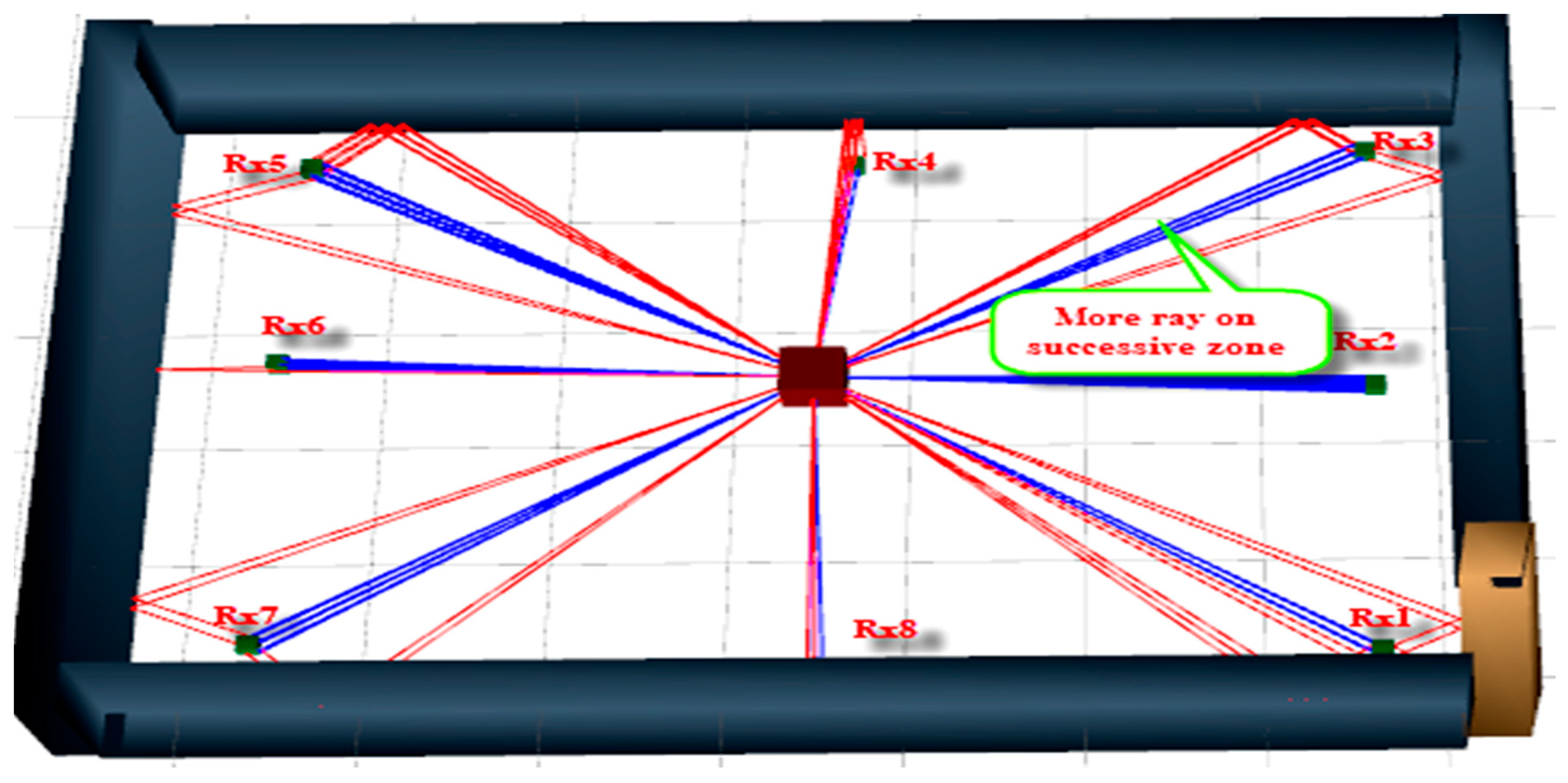
Figure 3 represents the RT simulation that has been performed using proposed methods among the 1 base station and eight mobile stations. Moreover, in this simulation, all the Rx gain enough LoS and NLoS rays for strong RSSI. It will be mentioned from Figure 3 that a probable angle wise launched rays have more contribution in mobile stations.

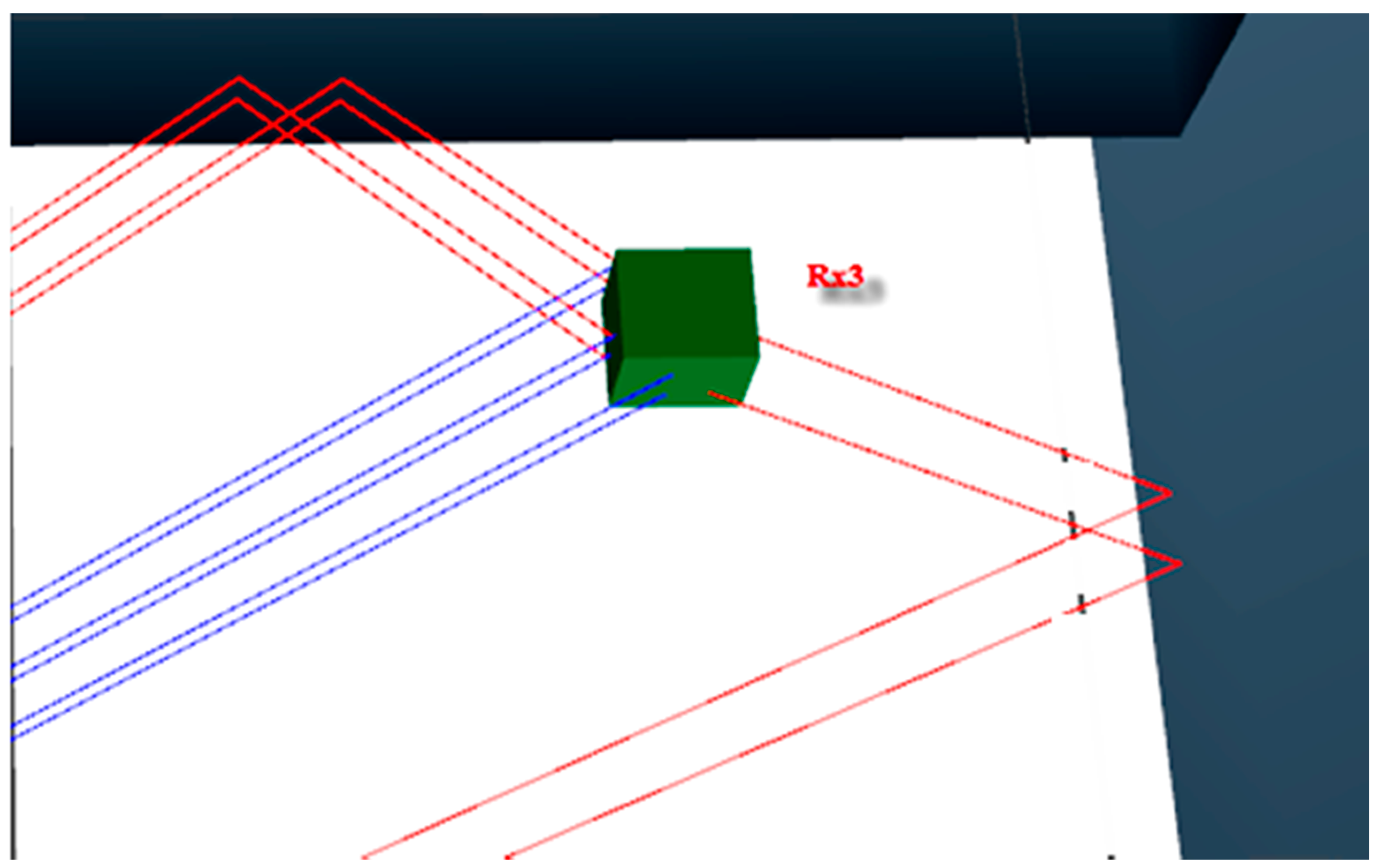
The Figure 4 represented the Rx3 mobile station from Figure 3 received multipath signals. The mobile station Rx3 were hit by six LoS and six NLoS ray multi-paths. Those are in the phase so the RSSI will be higher. In conclusion, the proposed method provides strong coverage to the RX, which is a current feature of higher mmW.

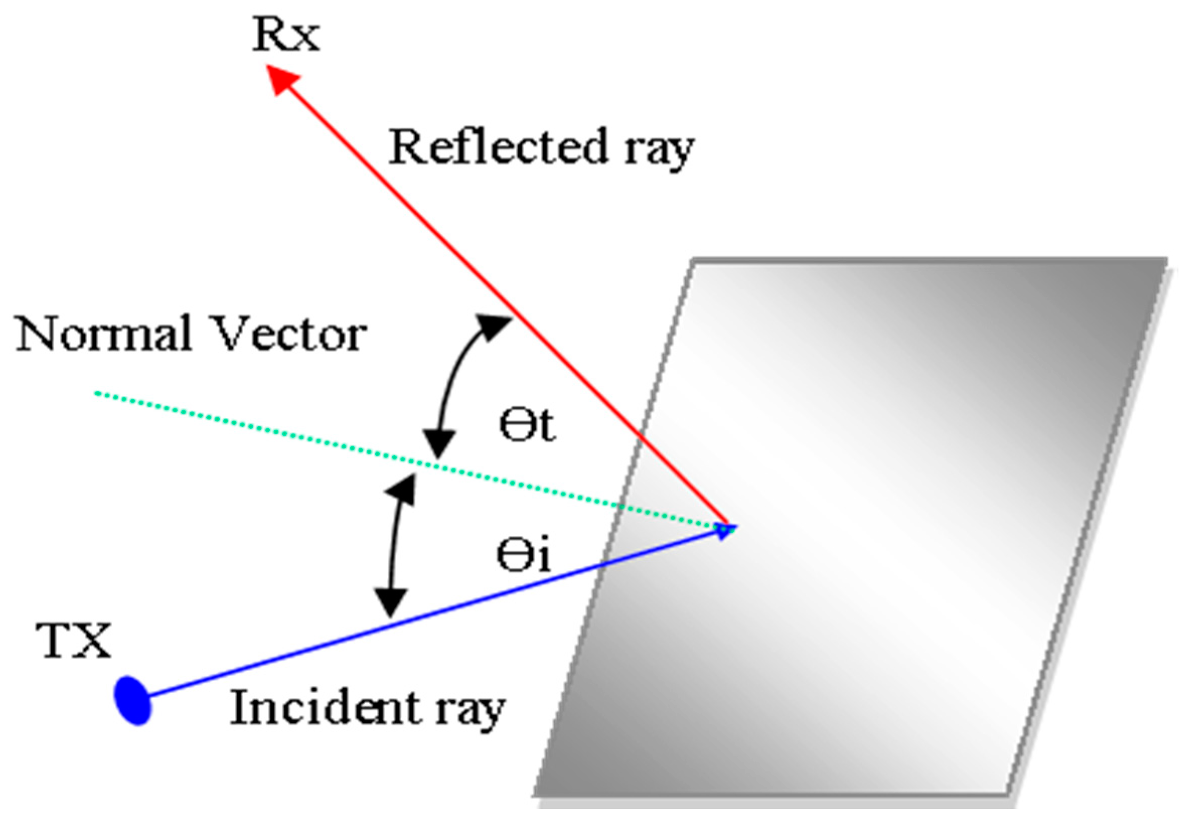
3.4. Reflection

The indoor scenario has a larger wall rather than a wavelength of mmW. In this circumstance, calculations of the refection coefficient have been performed using “Fresnel equation” [29]. According to this mathematical equation, reflection coefficients of both perpendicular and parallel polarizations are expressed by the symbol ${\mathsf{\Gamma }}_{\mathrm{s}}$ and ${\mathsf{\Gamma }}_{\mathrm{p}},$ respectively. The value of ${\mathsf{\Gamma }}_{\mathrm{s}}$ and ${\mathsf{\Gamma }}_{\mathrm{p}}$ are calculated using Equations (7) and (8) with respect for wave impedance.

$${\mathsf{\Gamma }}_{\mathrm{s}}=|\frac{{\mathrm{Z}}_2{\cos \mathsf{\theta }}_{\mathrm{i}}-{\mathrm{Z}}_1{\cos \mathsf{\theta }}_{\mathrm{t}}}{{\mathrm{Z}}_2{\cos \mathsf{\theta }}_{\mathrm{i}}+{\mathrm{Z}}_1{\cos \mathsf{\theta }}_{\mathrm{t}}}{|}^2$$

(7)

$${\mathsf{\Gamma }}_{\mathrm{p}}=|\frac{{\mathrm{Z}}_2{\cos \mathsf{\theta }}_{\mathrm{t}}-{\mathrm{Z}}_1{\cos \mathsf{\theta }}_{\mathrm{i}}}{{\mathrm{Z}}_2{\cos \mathsf{\theta }}_{\mathrm{t}}+{\mathrm{Z}}_1{\cos \mathsf{\theta }}_{\mathrm{i}}}{|}^2$$

(8)

The incident angle symbolized by ${\mathsf{\theta }}_{\mathrm{i}}$ and the refracted angle by ${\mathsf{\theta }}_{\mathrm{t}}$. The impedances of first and second media are expressed by ${\mathrm{Z}}_1$ and ${\mathrm{Z}}_2$. The impedance assessment depends on obstacle permittivity ${\mathsf{\epsilon }}_{\mathrm{r}}$. Furthermore, ${\mathsf{\mu }}_0$ symbolize the blank or non-magnetic media permeability of the building indoor properties. The conductivity σ presumed to be very few for non-conducting building resources such as concrete, brick, and glass. Figure 5 shows the graphical presentation of the reflection. The symbol σ means the conductibility, which is estimated to be very low for non-conducting indoor objects such as glass.

Moreover, a refracted dimension of media can be exchange by using “Snell’s law” with respect to the equation by incorporating the angle of refractive and incident.

$${\mathsf{\Gamma }}_{\mathrm{s}}=|\frac{{\cos \mathsf{\theta }}_{\mathrm{i}}-\sqrt{{\mathsf{\epsilon }}_{\mathrm{r}}-{\sin }^2{\mathsf{\theta }}_{\mathrm{i}}}}{{\cos \mathsf{\theta }}_{\mathrm{i}}+\sqrt{{\mathsf{\epsilon }}_{\mathrm{r}}-{\sin }^2{\mathsf{\theta }}_{\mathrm{i}}}}{|}^2$$

(9)

$${\mathsf{\Gamma }}_{\mathrm{p}}=|\frac{{\mathsf{\epsilon }}_{\mathrm{r}}{\cos \mathsf{\theta }}_{\mathrm{i}}-\sqrt{{\mathsf{\epsilon }}_{\mathrm{r}}-{\sin }^2{\mathsf{\theta }}_{\mathrm{i}}}}{{\mathsf{\epsilon }}_{\mathrm{r}}{\cos \mathsf{\theta }}_{\mathrm{i}}+\sqrt{{\mathsf{\epsilon }}_{\mathrm{r}}-{\sin }^2{\mathsf{\theta }}_{\mathrm{i}}}}{|}^2$$

(10)

Equations (9) and (10) are used to calculate coefficients values. Moreover, the parameters ${\theta }_i$ and ${\epsilon }_r$ estimate the reflection coefficient. The ${\epsilon }_r$ value depends on the frequency band of mmW and the indoor medium properties.

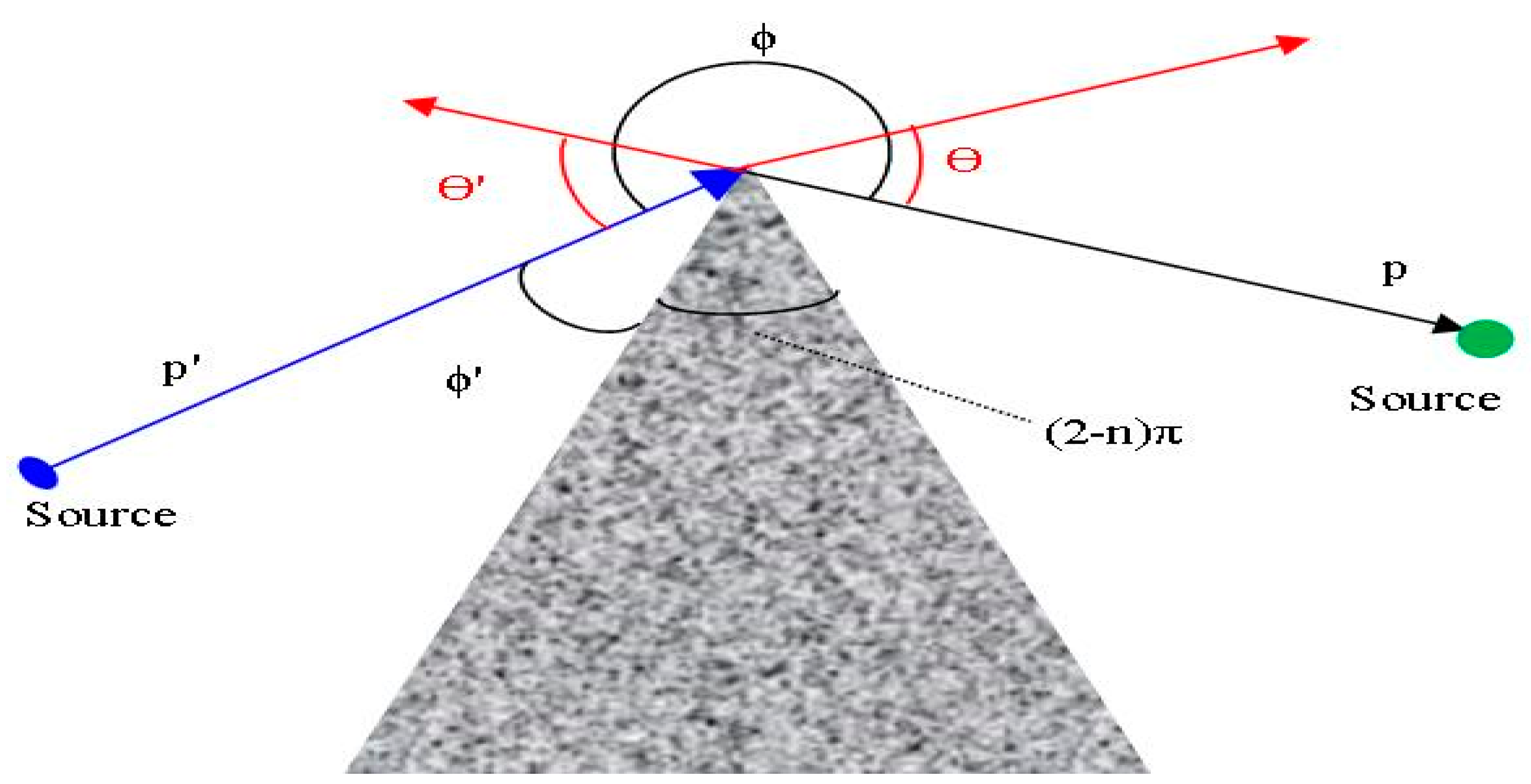
3.5. Diffraction

Vertical and horizontal diffraction coefficients are calculated by the wedge model [30]. Diffraction rays RSSI value is much lower than LoS even though the diffraction feature helps to reach the rays in the shadowed zone. Therefore, diffraction is considered as an important factor of WCS. The complexity of diffraction is high to implement in RT because diffraction points start producing a subordinate source to produce several diffracted rays. To overcome the complexity issue, estimate the diffraction coefficient by using the final version of the Luebber model [30,31]. As per UTD, point wise field $E_{GTD}$ is calculated using Equation (11) [32].

$$E_{GTD}=E_0\frac{e^{-jk{p}^{\prime }}}{p^{\prime }}{D}_{\perp }^{\parallel }\sqrt{\frac{p^{\prime }}{p\left(p^{\prime }+p\right)}}·e^{-jkp}$$

(11)

The term $E_0$ expresses amplitude of the starting point, k is used to mean the wave number, $p$ expressed the distance between the TX diffraction source point, the distance between Rx and the diffraction edge is expressed by $p^{\prime }$, and term $D_{\perp }^{\parallel }$ expresses the diffraction. The coefficient of non-conducting objects in every polarization has been calculated using Equation (12).

$$D_{\perp }^{\parallel }=\frac{-e^{-j\left(k\left(p+p^{\prime }\right)+\pi /4\right)}}{2n\sqrt{2\pi k}\mathit{sin}\beta }X\left\{\frac{F\left(kL{a}^{+}\left(\varphi -{\varphi }^{\prime }\right)\right)}{\mathit{tan}\left[\left(\pi +\varphi -{\varphi }^{\prime }\right)/2n\right]}+\frac{F\left(kL{a}^{-}\left(\varphi -{\varphi }^{\prime }\right)\right)}{\mathit{tan}\left[\left(\pi +\varphi -{\varphi }^{\prime }\right)/2n\right]}+{\mathsf{\Gamma }}_{\perp }^{0\parallel }\frac{F\left(kL{a}^{-}\left(\varphi +{\varphi }^{\prime }\right)\right)}{\mathit{tan}\left[\left(\pi +\varphi -{\varphi }^{\prime }\right)/2n\right]}+{\mathsf{\Gamma }}_{\perp }^{n\parallel }\frac{F\left(kL{a}^{+}\left(\varphi +{\varphi }^{\prime }\right)\right)}{\mathit{tan}\left[\left(\pi +\varphi +{\varphi }^{\prime }\right)/2n\right]}\right\}$$

(12)

The term ${\mathsf{\Gamma }}_{\perp }^{0\parallel }$ and ${\mathsf{\Gamma }}_{\perp }^{n\parallel }$ are used to express reflection coefficients for horizontal and vertical polarization. The incident angles and forward directions are expressed by $\varphi$ and backward directions by $n\pi -\varphi$, $L=\left(p{p}^{\prime }\left(p+p^{\prime }\right)\right),$ $a\pm \left(\beta \right)=2cos2\left[\left(2n\pi N\pm -\beta \right)\right]/2],\beta =\varphi \pm {\varphi }^{\prime },$ and $N\pm$ (see Equation (12)).

The graphical schematic views of diffraction with respect to several variables are presented in Figure 6. The simulation incorporated both side diffractions for each ray.

3.6. Ray Tracing Final Mathematical Equations

In simulations as per RT characteristics, reflections and diffraction are accrued with the ray before the ray reached the mobile stations. The term ${\mathrm{E}}_n$ expresses the electric field intensity, which can be calculated using Equation (13) [33].

$${\mathrm{E}}_n={\mathrm{E}}_{\mathrm{in}}\left(Q_n\right)\left({\displaystyle \prod }_{i=0}^{a_n}{R}_{in}{A}_{rin}\right)\left({\displaystyle \prod }_{j=0}^{b_n}{T}_{jn}{A}_{tjn}\right) \left({\displaystyle \prod }_{m=0}^{c_n}{D}_{mn}{A}_{dmn}\right)e^{-jk{s}_n}$$

(13)

The incident of the electric field for the first scattering is expressed by ${\mathrm{E}}_{\mathrm{in}}\left(Q_n\right)$. The symbols $a_n, b_n, and c_n$ are used to express the number of reflections, transmissions, and diffractions, which occurs sequentially. The symbols $R_{in}, T_{jn}, \mathrm{and} D_{mn}$ are used to express the associate dyadic reflection, the transmission, and diffraction coefficient consecutively. The symbols $A_{rin}, A_{tjn}, \mathrm{and} A_{dmnn}$ are used to express correlated spreading factors. The whole distance travel by the ray is expressed by S_n. Multichannel modeling mobile stations received several rays. The scenario wise total electric field intensity E_total is the subtotal of each ray, which is driven using Equation (14).

$${\mathrm{E}}_{total}={\displaystyle \sum }_{n=0}^M {\mathrm{E}}_{\mathrm{in}}\left(Q_n\right)\left({\displaystyle \prod }_{i=0}^{a_n}{R}_{in}{A}_{rin}\right)\left({\displaystyle \prod }_{j=0}^{b_n}{T}_{jn}{A}_{tjn}\right) \left({\displaystyle \prod }_{m=0}^{c_n}{D}_{mn}{A}_{dmn}\right)e^{-jk{s}_n}$$

(14)

The total number of rays that reached the mobile station is through M. The transmit power $P_t$, base station pattern, and $Q_n$ in RT is calculated to estimate ${\mathrm{E}}_{\mathrm{in}}\left(Q_n\right)$ by Equation (15).

$${\mathrm{E}}_{\mathrm{in}}\left(Q_n\right)=\frac{E_0\sqrt{G_m^{\prime }}}{p_n} {\tilde{a}}_m$$

(15)

The $E_0= \sqrt[ ]{\frac{n_0}{4\pi }}{P}_t{G}_t$ is the electric field intensity, which is estimated as one meter distance from the base station for antenna gain [33]. The symbol $n_0$ means the intrinsic impedance, $G_t$ means antenna directivity, $G_m^{\prime }$ and The ${\tilde{a}}_m$ express antenna gain and polarization in the direction of $Q_n$, respectively. The $p_n$ is the length of $Q_n$ from TX. The symbol ${\mathrm{E}}_n$ expresses the Rx field strength. The estimation of Vrn as voltage is based on the antenna and polarization of Rx. The Vrn is calculated by using Equation (16).

$$V_{rn}= \sqrt[ ]{\frac{{\lambda }^2{G}_{rn}{R}_0}{4\pi }}\left({\mathrm{E}}_n.{\tilde{a}}_{rm}\right)e^{j\varphi }$$

(16)

The symbol ${\lambda }^2$ expresses the wavelength. $G_{rn}$ symbolized Rx antenna gain in the ray angle of arrival, $R_0$ expresses Rx impedance, the symbol ${\tilde{a}}_{rm}$ expresses Rx polarization in the ray angle of arrival, and $e^{j\varphi }$ is the mean fixed-phase shift accessible by Rx. Lastly, the Rx RSSI is calculated by Equation (17) [34].

$$\begin{gathered} P_r=\frac{|{{\displaystyle \sum }}_{n=0}^M{V}_m{|}^2}{R_0} \\ =\frac{{\lambda }^2}{4\pi n_0}|{\displaystyle \sum }_{n=0}^M\left(E_n.{\tilde{a}}_{rn}\right)\sqrt{G_{rn}}{|}^2 \\ =\frac{{\lambda }^2}{4\pi n_0}|{\displaystyle \sum }_{n=0}^M \frac{E_0{e}^{-jk{s}_n}\sqrt{G_{rn}{G}_{tn}^{\prime }}}{P_n}{\tilde{a}}_{tn}\left({\displaystyle \prod }_{i=0}^{a_n}{R}_{in}{A}_{rin}\right)\left({\displaystyle \prod }_{j=0}^{b_n}{T}_{jn}{A}_{tjn}\right) \left({\displaystyle \prod }_{m=0}^{c_n}{D}_{mn}{A}_{dmn}\right){\tilde{a}}_{rn}{|}^2 \end{gathered}$$

(17)

The total valid path is express by M.

3.7. Simulation Parameter Configuration by Compilations of Electrical Properties of Materials

The material electrical properties such as permittivity and conductivity can be hard to find since characteristics are mentioned using different groupings of parameters. The permittivity and conductivity may be quoted with respect to frequencies.

The frequency ranges have limits but are suggestive from the measurements to derive the models. The frequency 1–100 GHz limits must not be exceeded. The Permittivity and Conductivity of the NWCC_P15a environment are given in

Table 3. Specifications of the experimental material properties [35,36,37].

Material Class	$\mathbf{Permittivity} \left({\mathit{ϵ}}_{\mathit{r}}\right)$	Conductivity (σ)
Concrete	5.31	0.0326
Brick	3.75	0.38
Plasterboard	2.94	0.0116
Wood	1.99	0.0047
Glass	6.27	0.0043
Ceiling board	1.50	0.0005
Chipboard	2.58	0.0217
Floorboard	3.66	0.0044

. Table 3 reported the major materials that need to be incorporated in the simulation per measurement.

4. Validation of Proposed RT Results

The proposed RT method simulation output validation is compared with the actual measurement and is presented in this section. Additionally, the proposed method is compared with the highly used conventional SBR method. The aim of this work is validated with the proposed method by the similar arrangement of measurements with respect to comparison results. The layout design incorporated walls including indoor furniture and more. The simulation has been performed on the layout using SBR and the proposed method by Telecom Malaysia, which included research and development through a funded in house developed software tool. Based on RT characteristics, most of the rays hit within the indoor objects. As rays hit with obstacles, reflection and tracing continued within the reflections limit. The simulation estimates the number of received rays by the receiver, the simulation time, RSSI, and PL of the mobile station [38]. The receiver sensitivity limit is −150 dB and it is configured in the simulation. The ray line between the Rx and TX will be removed depending on some conditions: the ray dose not reached the receiver spare, the number of reflections reaches the limit, and RSSI is below the receiver sensitivity.

The measurement is conducted at NWCC_P15a. The base on the measurement layout scenario simulations have been done using SBR and proposed RT methods. Mainly, windows transparent windows, doors, and walls are incorporated in the simulation layout. The RT simulation has been done using the standards values of permittivity and conducting regarding the object mentioned in Table 3. Some issues have been found to estimate the permittivity and conducting of objects such as a different wooden wall, different concrete, and ceiling. In this situation, estimated permittivity and conducting values of obstacles are given in Reference [39] and are used in the simulation. The base station is placed inside room 2 and several Rx are positioned in several places as per the measurement scenario. The different frequency has a different effect on obstacles and materials in WCS [40,41,42]. In this research, the standard values conductivity and permittivity are used for 38 GHz.

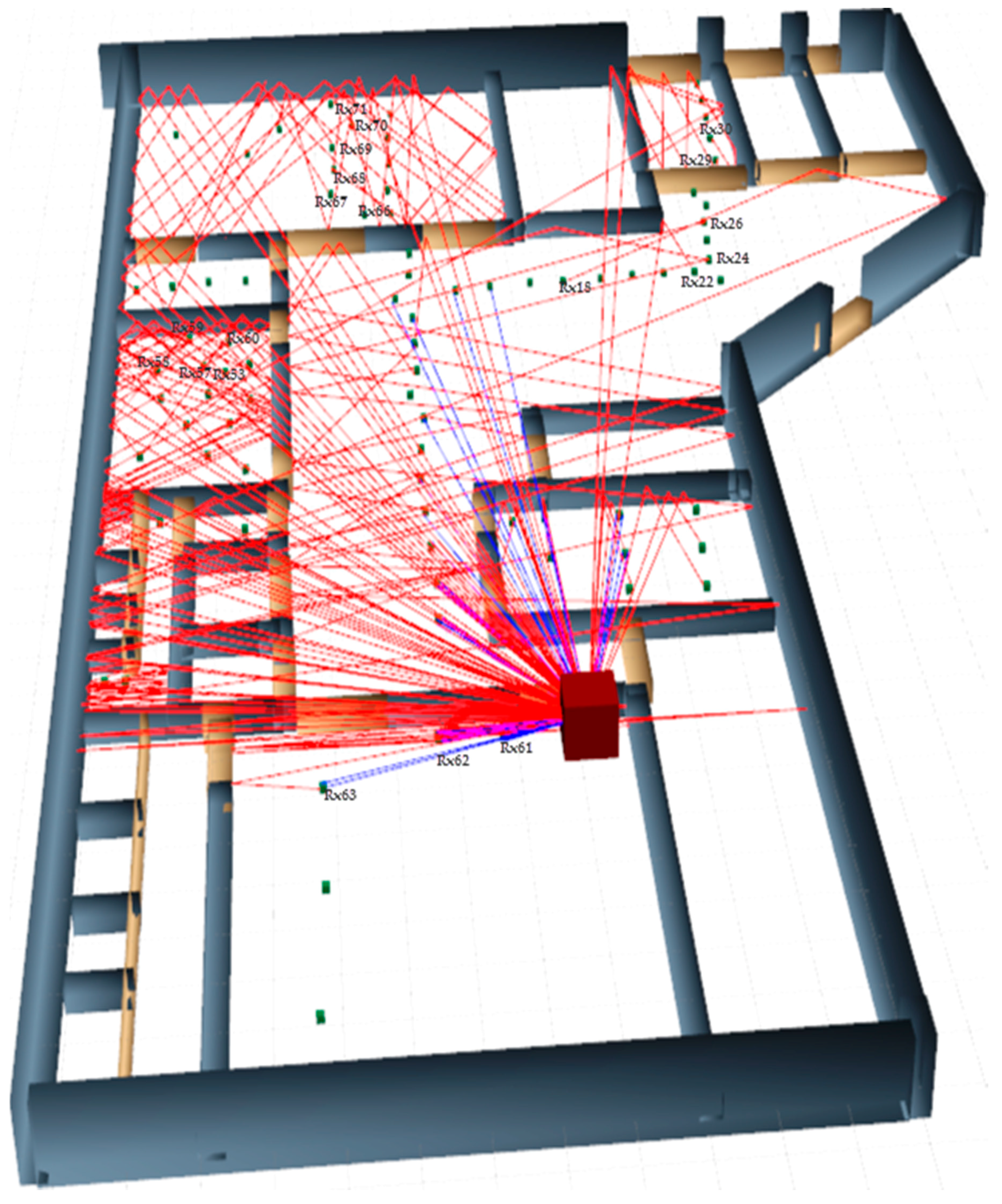
The graphical representation of the NWCC_P15a by the SBR method is presented in Figure 7. RT visualization in Figure 7 bear several reflections. Consequently, its PL and propagation times are higher and RSSI is lower. It is also noticeable that the coverage is not good because a few rays contributed in the Rx with most of them bearing higher reflections. If fewer rays contribute in Rx, then RSSI will be lower. Furthermore, Rx received several rays but most of them are because of reflections, which bear PL that reduce the RSSI. By observing the output of the SBR and measurement, we found that RSSI and PL has moderate agreement.

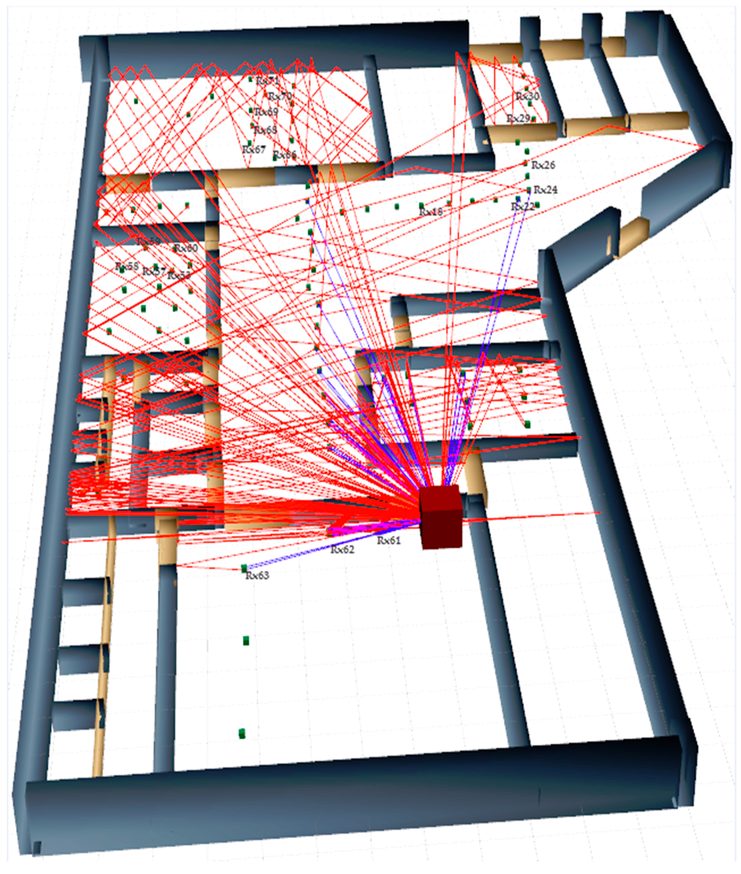
The graphical representation of the NWCC_P15a by the proposed method is presented in Figure 8. Since RT visualization in Figure 8 bear less reflections, its PL and propagation times are lower and RSSI is higher. The coverage is good because a large number of rays contributed in the Rx. Furthermore, Rx received several rays, which helped increase the RSSI. By observing the output of the proposed method and the measurement, RSSI and PL had considerable agreement.

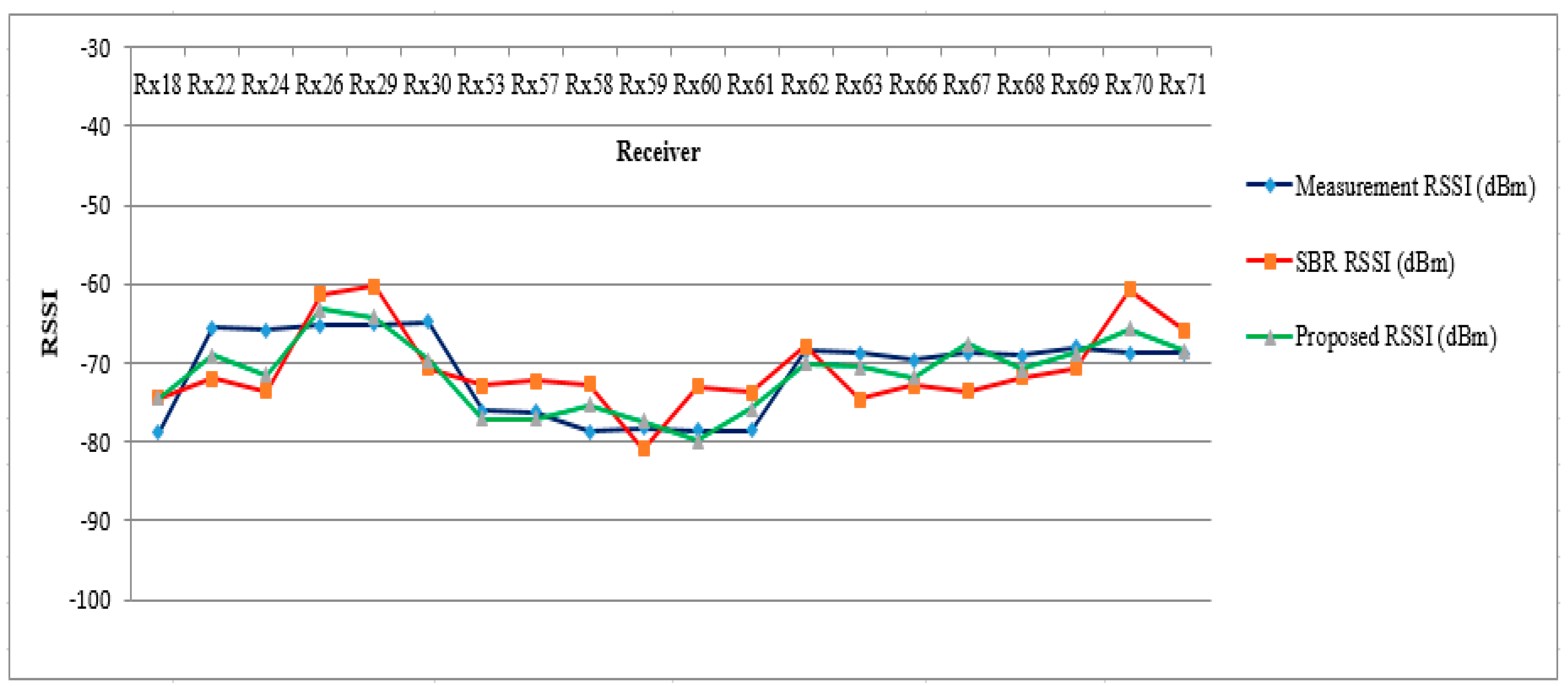
The RSSI Standard Deviation(SD) of the SBR method with the measurement is 1.79 for the NWCC_P15a scenario. The RSSI lowest and highest dissimilarity of the SBR method with measurements are 0.6 and 7.99 dBm, respectively. The highest dissimilarity RSSI is found to have an obstacle or the received rays bear several reflected rays. Correspondingly, the RSSI SD of the proposed method with the measurement is 1.46 for the same scenario. The SD value of the simulation with the measurement 1.46 is expressing the proposed method acceptable for RT modeling. The RSSI lowest and highest dissimilarity of the proposed method are 0.27 and 5.58 dBm, respectively. The highest dissimilarity RSSI is found due to an obstacle. Nevertheless, in the proposed method even in the worst-case scenario, the RSSI dissimilarity is considerable between the measurement and the proposed method simulation.

Figure 9 represents the comparison line graph of RSSI for the measurement, the SBR, and the proposed methods data. For this research, the measurement RSSI data are taken into account as standard data. The SBR method’s mobile stations Rx62, Rx69, Rx59, Rx68, and Rx71 shows the moderate relationship trend in RSSI with the measurement, respectively. The RSSI SD of SBR method and standard data is 0.86. Reversely, The SBR method’s mobile stations Rx66, Rx53, Rx26, Rx57, Rx18, Rx67, Rx61, Rx29, Rx60, Rx63, Rx30, Rx58, Rx22, Rx24, and Rx70 shows the distance relationship trend with the measurement, respectively. The RSSI SD of the SBR method with standard data is 1.38. Similarly, for the proposed method, mobile stations Rx71, Rx69, Rx59, Rx29, Rx57, Rx53, Rx67, Rx60, Rx63, Rx68, Rx26, Rx66, Rx61, and Rx70 show the good relationship trend in RSSI with the measurement. The RSSI SD of the proposed method with standard data is 0.75. Reversely, the proposed method’s mobile stations Rx22, Rx58, Rx18, Rx30, and Rx24 show the moderate relationship trend with the measurement. The RSSI SD of the proposed method with standard data is 0.83. Moreover, the proposed method maximum number of mobile stations except Rx24 shows very good agreement with standard data. With the comparative analysis, Figure 7, Figure 8 and Figure 9 for RSSI founded that the proposed method represented better agreement with the measurement when compared to the SBR method.

To reach the receiver, the ray has to travel some distance. Therefore, it bears PL, which reduce the RSSI. In WCS, PL has great impact in terms of modeling.

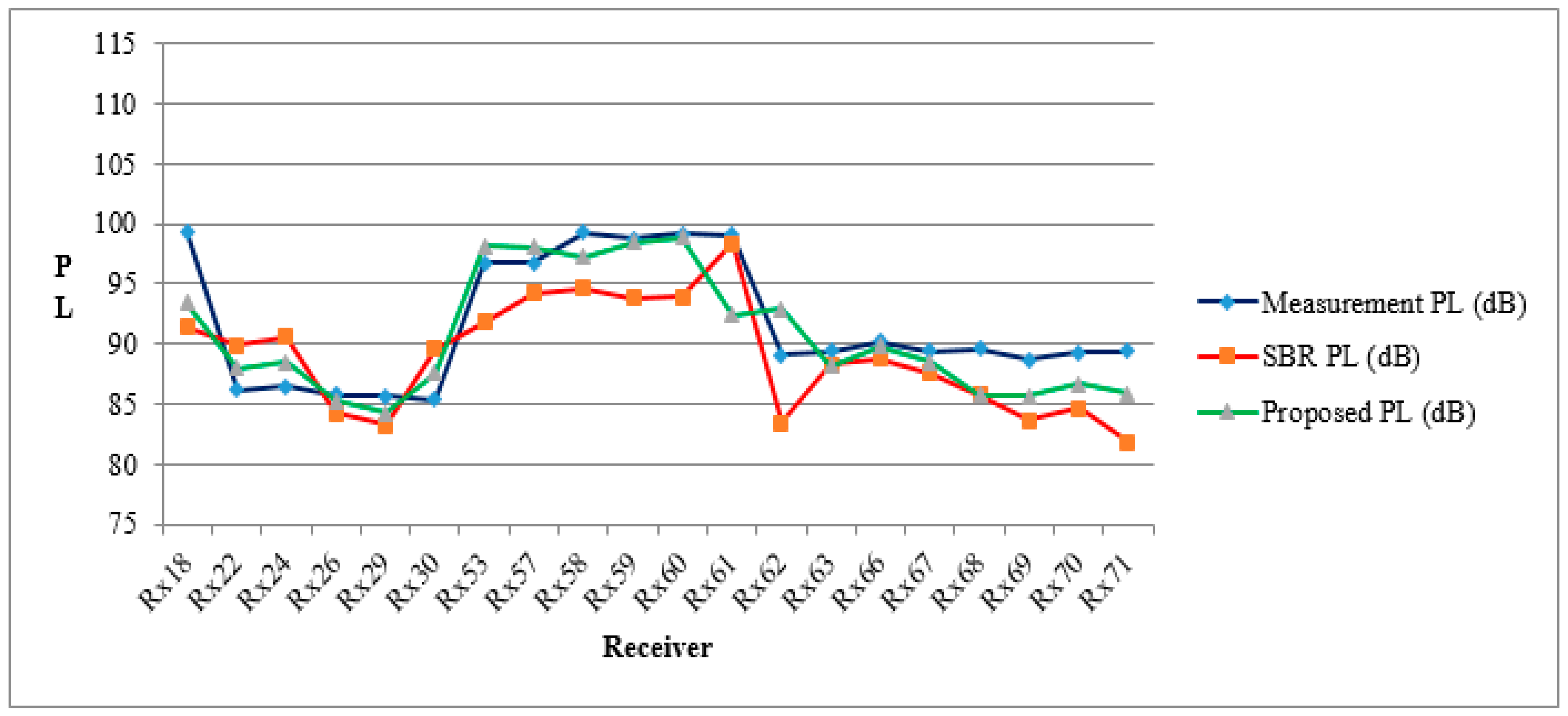
The PL SD of the SBR method with the measurement is 1.96 for the NWCC_P15a scenario. The PL lowest and highest dissimilarity of the SBR method with measurements are 0.71 and 7.99 dB, respectively. The highest dissimilarity PL is found to quickly appear or the received rays bear several reflected rays.

Correspondingly, the PL SD of the proposed method is 1.74 for the same scenario. The SD value 1.74 of the simulation is expressing the proposed method acceptable for RT modeling. The PL lowest and highest dissimilarity of the proposed are 0.32 and 6.69 dB, respectively. The highest dissimilarity PL is found due to an obstacle. Nevertheless, in the proposed method even in the worst-case scenario, the PL dissimilarity is considerable between the measurement and the proposed method simulation.

Figure 10 represented the comparison line graph of PL for measurement, SBR, and proposed methods data. For this research, the measurement PL data takes into account the standard data. The SBR method’s mobile stations Rx61, Rx63, Rx66, Rx26, Rx67, Rx29, and Rx57 show the moderate relationship trend in PL with measurements. The PL SD of SBR method with standard data is 0.62. Reversely, The SBR method’s mobile stations Rx22, Rx68, Rx24, Rx30, Rx70, Rx58, Rx53, Rx59, Rx69, Rx60, Rx62, Rx71, and Rx18 show the distance relationship trend with measurements, respectively. The PL SD of the SBR method with standard data is 1.26. Similarly, for the proposed method, mobile stations Rx60, Rx59, Rx66, Rx26, Rx67, Rx63, Rx57, Rx53, Rx29, Rx22, Rx24, Rx58, Rx30, and Rx70 show the good relationship trend in PL with the measurement, respectively. The RSSI SD of the proposed method with standard data is 0.71. Reversely, the proposed method’s mobile stations Rx69, Rx71, Rx68, Rx62, Rx18, and Rx61 show the moderate relationship trend in PL with the measurement. The PL SD of the proposed method with standard data is 1.35. Moreover, the proposed method maximum number of mobile stations except Rx61 shows very good agreement with standard data. With respect to the good similarity of simulation by using PL SD with standard data less than 1: seven numbers of Rx are found in SBR and fourteen numbers of Rx are found in the proposed method. On the other hand, fewer similarity of simulation by using PL SD with standard data greater than 1: thirteen numbers of Rx are found in SBR, and six Rx are found in the proposed method. With the comparative analysis in Figure 7, Figure 8, and Figure 10 for PL, the proposed method represented better agreement with the measurement than the SBR method.

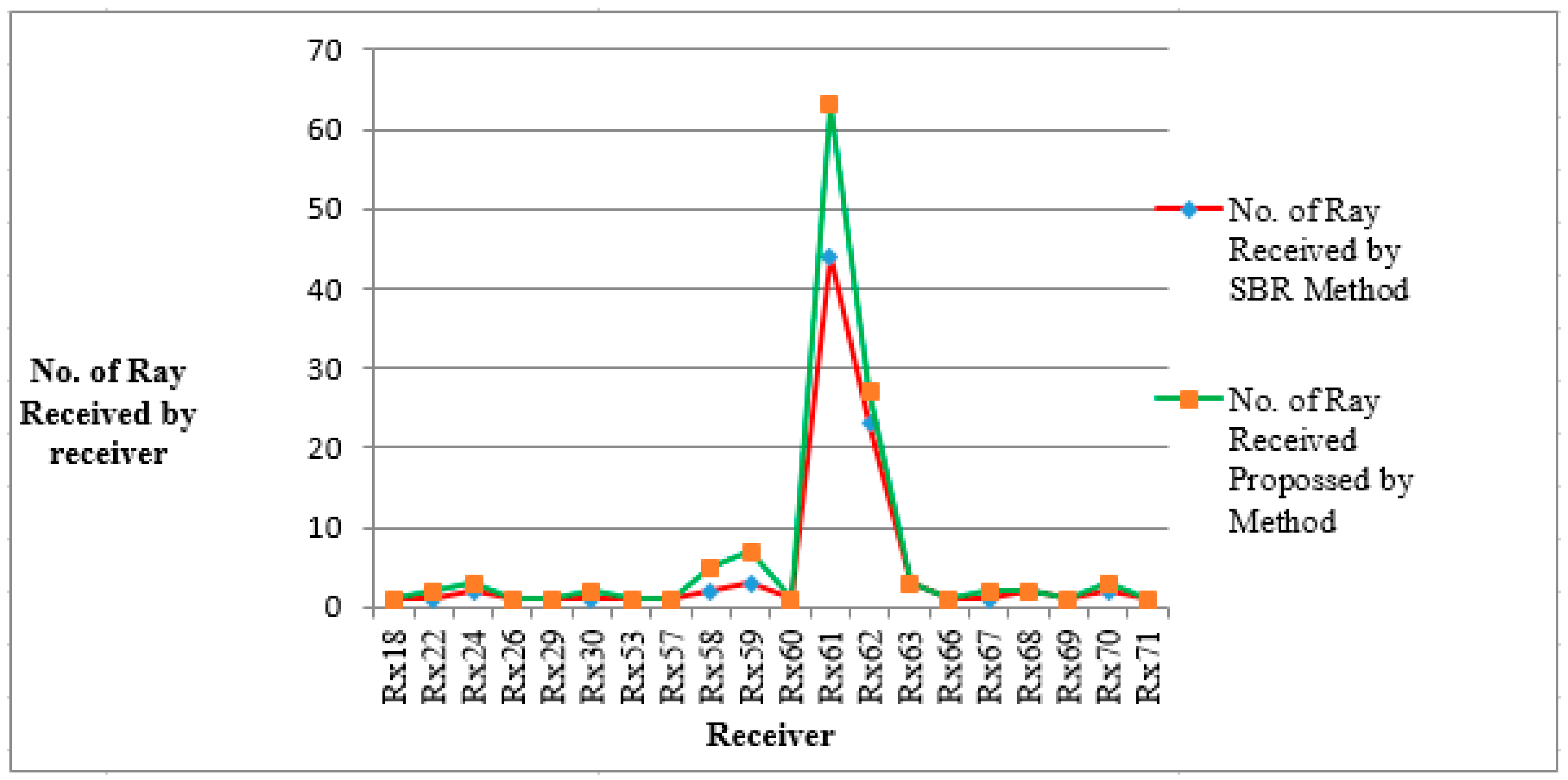
Figure 11 represented the line graph regarding the receiver and the number of contributed rays in the SBR and the proposed method. This type of data is not available in the measurement, so a comparison has been performed between the SBR and the proposed method data. The mobile station Rx61 received the maximum number of rays in both simulations. For the case of the SBR method, this receiver received 44 rays, which is similar to the proposed method in which this receiver received 63 rays. As per the overview from Figure 11, in the proposed method, a higher number of rays reached the mobile station rather than the SBR method.

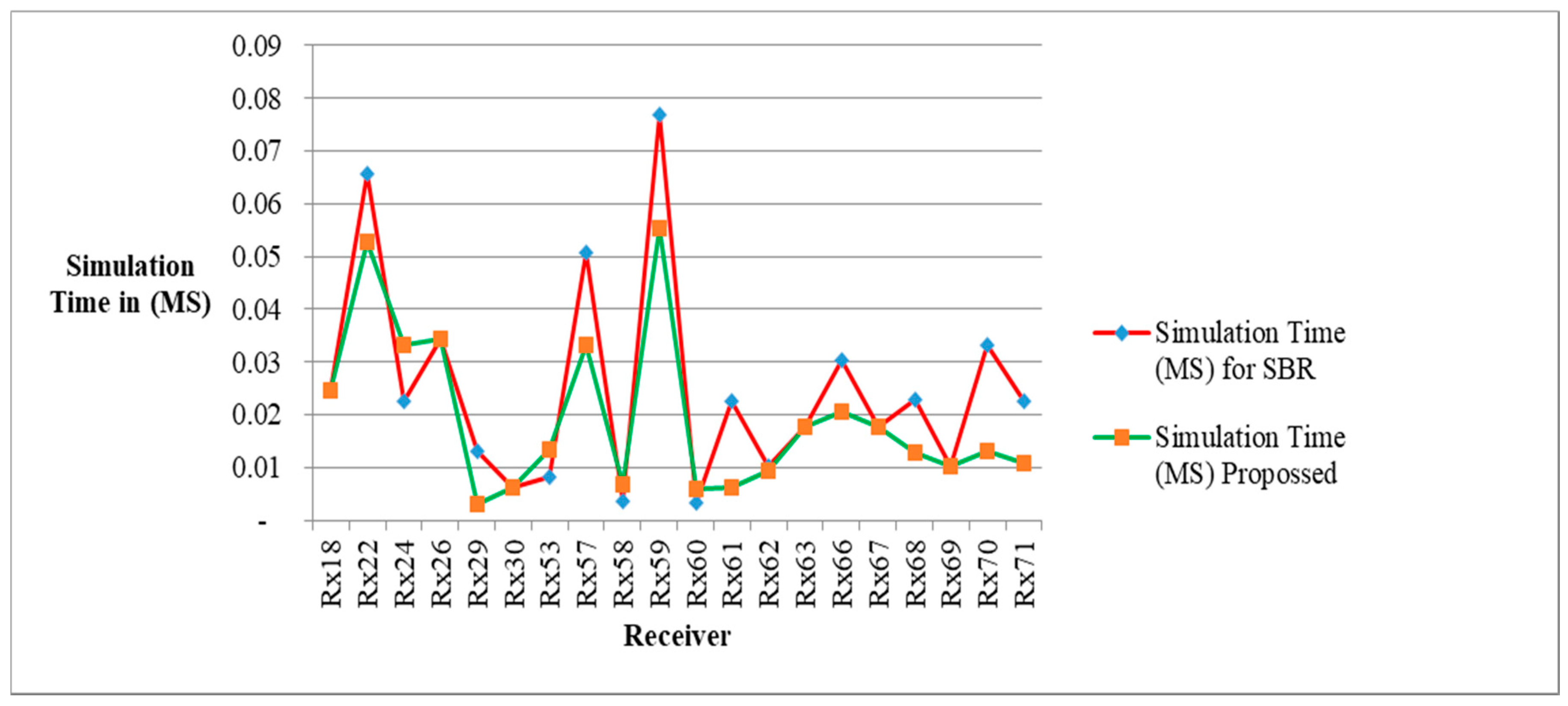
Figure 12 represented the line graph of the mobile station and the simulation time for both the SBR and proposed methods. The SBR method bears high computational time when compared to the proposed method. This simulation has been run using high configuration with a good graphics server. In a normal computer, this simulation time will be much higher than in this scenario.

In the proposed method, the ray-launching phase has significant contribution in the simulation. Consequently, RL is the first phase of RT [43]. Proper utilization of RL makes the proposed method more capable, suitable, and intelligent [44]. Few ray launchings are done in the proposed method rather than SBR. To get sufficient coverage using few numbers of launched rays in the predefined potential region is the outstanding contribution of the proposed method. Lastly, the proposed method has a very significant contribution in the WCS base on the coverage, RL, simulation time, PL, and RSSI.

5. Conclusions

In this paper, we have presented an extensive measurement and a full 3-D RT proposed method simulation in order to investigate mmW for indoor radio propagation at 38 GHz. Although the practical measurement provides accurate justification of performance, it badly needs huge amount of time, effort, and cost. While higher demand of mmW exists, relatively limited work has been done on it. In this circumstance, to bridge this gap, a smart RT simulator has been developed in this research using a proposed method and an SBR method. The conventional SBR and proposed method are used in simulation based on GO and UTD. In the proposed method, more rays are launched in some potential zone and not in all directions, which minimizes the computational complexity without dropping valid paths between TX and Rx. Additionally, the proposed method coverage and propagation time also compared with the conventional SBR method. Mainly, good coverage and better propagation time is reported in the proposed method rather than the SBR method. The proposed method has been validated by comparing the results with a measurement campaign data, which has been done in the NWCC_P15a building basement floor at UTM, JB campus, Malaysia. For the validation purpose, a proposed method simulation result of RSSI, PL is compared with the measurement. Furthermore, for justification of the novelty of the proposed method, the existing SBR method output is analyzed with the same measurement data. Lastly, based on the effective analysis among the SBR, proposed method, and measurement output, the proposed method agrees with the measurement rather than the SBR. The information presented in this paper is expected to be helpful in future research of 38 GHz mmW for indoor WCS. The proposed algorithm in this manuscript could be implemented on GPU in future research for robustness. For future work, the proposed method from this study will be extended for outdoor ray tracing. More research is needed to further improve the speed and accuracy of the proposed method in a crowded scenario.

References

- Smulders, P. Exploiting the 60 GHz band for local wireless multimedia access: Prospects and future directions. IEEE Commun. Mag. 2002, 40, 140–147. [Google Scholar] [CrossRef]
- Forecast, C.V. Cisco Visual Networking Index: Global Mobile Data Traffic Forecast Update, 2016–2021 White Paper; Cisco Public Inf.: San Jose, CA, USA, 2017; Volume 1, pp. 1–35. [Google Scholar]
- Li, X.; Li, Y.; Li, B. The Diffraction Research of Cylindrical Block Effect Based on Indoor 45 GHz Millimeter Wave Measurements. Information 2017, 8, 50. [Google Scholar] [Green Version]
- Tsiropoulou, E.E.; Kapoukakis, A.; Papavassiliou, S. Energy-efficient subcarrier allocation in SC-FDMA wireless networks based on multilateral model of bargaining. In Proceedings of the 2013 IFIP Networking Conference, Brooklyn, NY, USA, 22–24 May 2013; pp. 1–9. [Google Scholar]
- Tsiropoulou, E.E.; Kapoukakis, A.; Papavassiliou, S. Uplink resource allocation in sc-fdma wireless networks: A survey and taxonomy. Comput. Netw. 2016, 96, 1–28. [Google Scholar] [CrossRef]
- Tsiropoulou, E.E.; Mitsis, G.; Papavassiliou, S. Interest-aware energy collection & resource management in machine to machine communications. Ad Hoc Netw. 2018, 68, 48–57. [Google Scholar] [CrossRef]
- Freeman, R.L. Radio System Design for Telecommunications (1–100 GHz); Wiley: New York, NY, USA, 1987. [Google Scholar]
- Crane, R.K. Electromagnetic Wave Propagation through Rain; Wiley: New York, NY, USA, 1996. [Google Scholar]
- Chou, S.-F.; Chao, H.-L.; Liu, C.-L. An efficient measurement report mechanism for Long Term Evolution networks. In Proceedings of the 2011 IEEE 22nd International Symposium on Personal, Indoor and Mobile Radio Communications, Toronto, Canada, 11–14 September 2011. [Google Scholar] [CrossRef]
- Sulyman, A.I.; Nassar, A.T.; Samimi, M.K.; MacCartney, G.R.; Rappaport, T.S.; Alsanie, A. Radio propagation path loss models for 5g cellular networks in the 28 GHz and 38 GHz millimeter-wave bands. IEEE Commun. Mag. 2014, 52, 78–86. [Google Scholar] [CrossRef]
- Akdeniz, M.R.; Liu, Y.; Rangan, S.; Erkip, E. Millimeter wave picocellular system evaluation for urban deployments. In Proceedings of the 2013 IEEE Globecom Workshops (GC Wkshps), Atlanta, GA, USA, 9–13 December 2013. [Google Scholar] [CrossRef]
- Rangan, S.; Rappaport, T.S.; Erkip, E. Millimeter-wave cellular wireless networks: Potentials and challenges. Proc. IEEE 2014, 102, 366–385. [Google Scholar] [CrossRef]
- Geok, T.K.; Hossain, F.; Kamaruddin, M.N.; Rahman, N.Z.A.; Thiagarajah, S.; Chiat, A.T.W.; Liew, C.P. A Comprehensive Review of Efficient Ray-Tracing Techniques for Wireless Communication. Int. J. Commun. Antenna Propag. 2018, 8, 123–136. [Google Scholar] [CrossRef]
- Jung, J.-H.; Lee, J.; Lee, J.-H.; Kim, Y.-H.; Kim, S.-C. Ray-tracing aided modeling of user-shadowing effects in indoor wireless channels. IEEE Trans. Antennas Propag. 2014, 62, 3412–3416. [Google Scholar] [CrossRef]
- McKown, J.W.; Hamilton, R.L., Jr. Ray tracing as a design tool for radio networks. IEEE Netw. 1991, 5, 27–30. [Google Scholar] [CrossRef]
- Rizk, K.; Wagen, J.-F.; Gardiol, F. Two-dimensional ray-tracing modeling for propagation prediction in microcellular environments. IEEE Trans. Veh. Technol. 1997, 46, 508–518. [Google Scholar] [CrossRef]
- Sato, H.S.; Otoi, K. Electromagnetic Wave Propagation Estimation by 3-D. In SBR Method. In Proceedings of the International Conference on Electromagnetics in Advanced Applications, Torino, Italy, 17–21 September 2007; pp. 129–132. [Google Scholar] [CrossRef]
- Shi, D.; Tang, X.; Wang, C. The acceleration of the shooting and bouncing ray tracing method on GPUs. In Proceedings of the 2017 General Assembly and Scientific Symposium of the International Union of Radio Science (URSI GASS), Montreal, QC, Canada, 19–26 August 2017; pp. 1–3. [Google Scholar] [CrossRef]
- Zhang, Z.; Ryu, J.; Subramanian, S.; Sampath, A. Coverage and channel characteristics of millimeter wave band using ray tracing. In Proceedings of the IEEE International Conference on Communications (ICC), London, UK, 8–12 June 2015; pp. 1380–1385. [Google Scholar]
- Chang, Y.; Baek, S.; Hur, S.; Mok, Y.; Lee, Y. A novel dual-slope mm-Wave channel model based on 3D ray-tracing in urban environments. In Proceedings of the 2014 IEEE 25th Annual International Symposium on Personal, Indoor, and Mobile Radio Communication (PIMRC), Washington, DC, USA, 2–5 September 2014; pp. 222–226. [Google Scholar]
- Hur, S.; Baek, S.; Kim, B.C.; Park, J.H.; Molisch, A.F.; Haneda, K.; Peter, M. 28 GHz channel modeling using 3D ray-tracing in urban environments. In Proceedings of the 2015 9th European Conference on Antennas and Propagation (EuCAP), Lisbon, Portugal, 13–17 April 2015; pp. 1–5. [Google Scholar]
- Samimi, M.K.; Rappaport, T.S. Statistical Channel Model with Multi-Frequency and Arbitrary Antenna Beamwidth for Millimeter-Wave Outdoor Communications. In Proceedings of the 2015 IEEE Globecom Workshops (GC Wkshps), San Diego, CA, USA, 6–10 December 2015; pp. 1–7. [Google Scholar] [CrossRef]
- Cassioli, D.; Win, M.Z.; Molisch, A.F. The ultra-wide bandwidth indoor channel: From statistical model to simulations. IEEE J. Sel. Areas Commun. 2002, 20, 1247–1257. [Google Scholar] [CrossRef]
- Rappaport, T.S.; MacCartney, G.R.; Samimi, M.K.; Sun, S. Wideband Millimeter-Wave Propagation Measurements and Channel Models for Future Wireless Communication System Design. IEEE Trans. Commun. 2015, 63, 3029–3056. [Google Scholar] [CrossRef]
- Maccartney, G.R.; Rappaport, T.S.; Sun, S.; Deng, S. Indoor Office Wideband Millimeter-Wave Propagation Measurements and Channel Models at 28 and 73 GHz for Ultra-Dense 5G Wireless Networks. IEEE Access. 2015, 3, 2388–2424. [Google Scholar] [CrossRef]
- Al-Samman, A.M.; Rahman, T.A.; Azmi, M.H.; Hindia, M.N.; Khan, I.; Hanafi, E. Statistical Modelling and Characterization of Experimental mm-Wave Indoor Channels for Future 5G Wireless Communication Networks. PLoS ONE 2016, 11, E0163034. [Google Scholar] [CrossRef] [PubMed]
- Ling, H.; Chou, R.C.; Lee, S.W. Shooting and Bouncing Rays: Calculating the RCS of an arbitrarily shaped cavity. IEEE Trans. Antennas Propag. 1989, 37, 194–205. [Google Scholar] [CrossRef]
- Baldauf, J.; Lee, S.W.; Lin, L.; Jeng, S.K.; Scarborough, S.M.; Yu, C.L. High frequency scattering from trihedral comer reflectors and other benchmark targets: SBR VS experiments. IEEE Trans. Antennas Propag. 1991, 39, 1345–1351. [Google Scholar] [CrossRef]
- Rappaport, T.S. Wireless Communications: Principles and Practice; Prentice-Hall: Englewood Cliffs, NJ, USA, 1996; Volume 2. [Google Scholar]
- Luebbers, R.J. Finite conductivity uniform GTD versus knife edge diffraction in prediction of propagation path loss. IEEE Trans. Antennas Propag. 1984, AP-32, 70–76. [Google Scholar] [CrossRef]
- Kouyoumjian, R.G.; Pathak, P.H. A uniform geometrical theory of diffraction for an edge in a perfectly conducting surface. Proc. IEEE 1974, 62, 1448–1461. [Google Scholar] [CrossRef]
- Keller, J.B. Geometrical theory of diffraction. J. Opt. Soc. Am. 1962, 52, 116–130. [Google Scholar] [CrossRef] [PubMed]
- Seidel, S.Y.; Rappaport, T.S. Site-specific propagation prediction for wireless in-building personal communication system design. IEEE Trans. Veh. Technol. 1994, 43, 879–891. [Google Scholar] [CrossRef] [Green Version]
- Mohtashami, V.; Shishegar, A.A. Effects of geometrical uncertainties on ray tracing results for site-specific indoor propagation modeling. In Proceedings of the 2013 IEEE-APS Topical Conference on Antennas and Propagation in Wireless Communications (APWC), Torino, Italy, 9–13 September 2013. [Google Scholar]
- Li, W.; Qian, Z.; Li, H. Interpretation and classification of P-series recommendation in ITU-R. Int. J. Commun. Netw. Syst. Sci. 2016, 9, 117–125. [Google Scholar] [CrossRef]
- AlAbdullah, A.A.; Ali, N.; Obeidat, H.; Abd-Alhmeed, R.A.; Jones, S. Indoor millimetre-wave propagation channel simulations at 28, 39, 60 and 73 GHz for 5G wireless networks. In Proceedings of the Internet Technologies and Applications (ITA), Wrexham, UK, 12–15 September 2017; pp. 235–239. [Google Scholar] [CrossRef]
- Mubarakah, N.; Sagala, R.S.; Prayitno, H. Wifi-friendly building, enabling wifi signal indoor: An initial study. In IOP Conference Series: Earth and Environmental Science; IOP Publishing: Bristol, UK, 2018; Volume 126. [Google Scholar]
- Remcom. Wireless InSite Reference Manual, ver. 2.7.1; Commercial SW User-Manual; Remcom Inc.: State College, PA, USA, 2014. [Google Scholar]
- ITU-R. Effects of Building Materials and Structures on Radio Wave Propagation above about 100 MHz; Technical report; Electronic Publication: Geneva, Switzerland, 2015. [Google Scholar]
- ITU-R. Effects of Building Materials and Structures on Radio Wave Propagation above about 100 MHz; International Telecommunication Union Radio Communication Sector: Geneva, Switzerland, 2013. [Google Scholar]
- Correia, L.M.; Frances, P.O. Estimation of materials characteristics from power measurements at 60 GHz. In Proceedings of the 5th IEEE International Symposium on Personal, Indoor and Mobile Radio Communications, Wireless Networks—Catching the Mobile Future., The Hague, The Netherlands, 18–23 September 1994; pp. 510–513. [Google Scholar]
- Lott, M.; Forkel, I. A multi-wall-and-floor model for indoor radio propagation. In Proceedings of the IEEE VTS 53rd Vehicular Technology Conference (Cat. No.01CH37202), Rhodes, Greece, 6–9 May 2001; pp. 464–468. [Google Scholar]
- Hong, Q.; Zhang, J.; Zheng, H.; Li, H.; Hu, H.; Zhang, B.; Lai, Z.; Zhang, J. The Impact of Antenna Height on 3D Channel: A Ray Launching Based Analysis. Electronics 2018, 7, 2. [Google Scholar] [CrossRef]
- Geok, T.K.; Hossain, F.; Chiat, A.T.W. A novel 3D ray launching technique for radio propagation prediction in indoor environments. PLoS ONE 2018. [Google Scholar] [CrossRef] [PubMed]
Figure 1.
SBR method graphical representation.
Figure 2.
RT simulation graphical view using the SBR method.
Figure 3.
RT simulation graphical view using a proposed method.
Figure 4.
Zoomed representation of the Rx3 mobile station of Figure 3.
Figure 5.
Geometric representation of the reflection.
Figure 6.
Schematic of cone diffraction.
Figure 7.
Simulation of NWCC_P15a layout using the SBR method.
Figure 8.
Simulation of NWCC_P15a layout using the proposed method.
Figure 9.
The measurement and SBR proposed methods and RSSI methods comparison graph.
Figure 10.
The PL comparison line graph among the output of measurement and SBR proposed methods.
Figure 11.
The comparison of the number of rays received in the graph between the SBR and proposed methods.
Figure 12.
The comparison of the simulation time graph between the SBR and the proposed methods.