A GL Model on Thermo-Elastic Interaction in a Poroelastic Material Using Finite Element Method


1
Nonlinear Analysis and Applied Mathematics Research Group (NAAM), Mathematics Department, King Abdulaziz University, Jeddah 21589, Saudi Arabia
2
Mathematics Department, Faculty of Science, Sohag University, Sohag 82524, Egypt
3
Department of Mathematics and Computer Science, Transilvania University of Brasov, Brasov 500093, Romania
*
Author to whom correspondence should be addressed.
Symmetry 2020, 12(3), 488; https://doi.org/10.3390/sym12030488
Submission received: 7 March 2020
/
Revised: 17 March 2020
/
Accepted: 20 March 2020
/
Published: 24 March 2020
(This article belongs to the Special Issue Composite Structures with Symmetry)
Abstract
:The purpose of this study is to provide a method to investigate the effects of thermal relaxation times in a poroelastic material by using the finite element method. The formulations are applied under the Green and Lindsay model, with four thermal relaxation times. Due to the complex governing equation, the finite element method has been used to solve these problems. All physical quantities are presented as symmetric and asymmetric tensors. The effects of thermal relaxation times and porosity in a poro-thermoelastic medium are studied. Numerical computations for temperatures, displacements and stresses for the liquid and the solid are presented graphically.
1. Introduction
The theory of poroelasticity was expanded by Biot [1]. Biot [2,3] formulated a theoretical framework for the propagation of isothermal waves in the fluid-saturated elastic porous medium for both cases of low- and high-frequency ranges. Following Biot’s model, many researchers have studied problems with the propagation of plane and surface wave in liquid-saturated porous mediums. Due to numerous applications in the fields of geophysics and similar subjects, growing attentiveness is being paid to the interactions between fluids such as water and thermo-elastic solids, a field of porothermoelasticity. Over the past four decades, thermoelastic models, which admit finite speed for thermal signals, have received a lot of attention. These models are known as generalized thermoelastic models. Lord and Shulman [4] have obtained the first generalized thermoelastic model with one thermal relaxation time, while Green-Lindsay [5] presented the second generalized thermoelastic model with two relaxation times. The field of porothermoelasticity has many applications, especially in the study of the effects of the use of waste on the disintegrations of the asphalt concrete mix. The thermo-mechanical coupling in the poroelastic material is more complex as compared to the classical cases, due to the fact that the mechanical and thermal coupling occurs between the fluid and solid phases. Following [3], many researchers including [6,7,8,9] have contributed towards various problems in porothermoelastic medium. Abbas [10] studied the natural frequencies of a poroelastic hollow cylinder. Schanz and Cheng [11] have studied the transient wave propagation in a one-dimensional poroelastic column. El-Naggar et al. [12] studied the effects of voids, initial stress, rotation and magnetic field on plane waves under generalized thermoelastic theory. Abbas et al. [13] have investigated the effects of thermal dispersion on free convection in a fluid-saturated porous media. Many researchers [14,15,16,17,18] have applied the generalized thermoelastic theories to get the numerical and analytical solutions of physical quantities. Marin et al. [19] have presented the effects of a dipolar structure under Green–Naghdi thermo-elasticity. Sur et al. [20] investigated the effects of memory on thermal wave propagations in an elastic solid with voids. Not reported in literature yet, it will be an interesting case to study the effects of thermal relaxation times in the propagations of waves in a generalized porothermoelastic medium. Many authors [21,22,23,24,25,26,27] have solved various problems under generalized thermo-elastics models and [28,29,30,31,32,33] have solved several problems for porous medium under different boundary conditions.
This paper explores the numerical solutions of the temperatures, displacements and stresses of the poro-thermoelastic medium, using the finite element method. For the considered variables, the numerical results are obtained and presented graphically, to show the effects of the porosity and the thermal relaxation times.
2. Basic Equations
Consider an isotropic, homogeneous and elastic medium with voids; the basic equations are based on [8,34], with Green-Lindsay [5] models in the absence of heat source, and body force can be expressed by
The constitutive equations
There are different three models as:
- (CT) points to the classical dynamical coupled theory
- (LS) points to Lord and Shulman’s model
- (GL) points to Green and Lindsay’s modelwhere are the thermal relaxation times of the solid and fluid phases, respectively, are the stress components applied to the solid surface, are the poroelastic coefficients, are the thermal and mixed asymmetric coefficients, is the reference temperature, is the fluid temperature increment, is the temperature increment of the solid, are the displacements of the solid and fluid phases, is the porosity of the material, is the interface coefficient of the interphase heat conduction, is the fluid phase thermal conductivity, is the solid thermal conductivity, are the thermal conductivity of the solid and the fluid, is the solid phase density per unit volume of bulk, is the density of the solid phase per unit volume of bulk, are the solid and the liquid densities, is the dynamics coupling coefficient, is the fluid phase mass coefficient, is the solid phase mass coefficient, are the strain of the fluid phase components, are the strain of the solid phase components, is the normal stress applied to the fluid surface, are the specific heat of the fluid and the solid phases, are the thermoelastic couplings between the phases, are the thermal expansion of the phases coefficients, is the specific heat couplings between the fluid and the solid phases, is the thermal viscosity of the fluid, is the thermal viscosity of the solid, is the couplings thermal viscosity between the phases, with the asymmetric coefficients , , , , , , , and .
We shall consider an isotropic, homogeneous and porothermoelastic medium occupying the region . For the one-dimensional problem, all the functions considered will depend only on the variables of space and . The components of displacements can be written by:
Then, the governing equations can be defined as
3. Initial and Boundary Conditions
The initial can be expressed as
While there are two types of boundary conditions, as
1. The thermal boundary conditions
The plane surface boundary of the middle at has been thermally loaded by thermal shock by the following:
where is constant and is the Heaviside unite step function.
2. The mechanical boundary conditions
The bounding surface plane of the middle at has been connected to tractions free on this surface, i.e.,
For convenience, the dimensionless variables can be written by
where and .
In terms of these non-dimensional forms of variables in (19), the above equations can be expressed as (the script has been neglected for its suitability)
where
- , , , , , , , , ,
- , , , , ,
4. Finite Element Method
In this section, the complex equations of wave propagation in a poroelastic medium are abbreviated by the finite element method (FEM). The finite element technique has been used here to obtain the solutions of Equations (20)–(23) under the boundary and initial conditions (26)–(29). This method is an originally advanced method and powerful for numerical solutions to complex problems in many fields and is the process of choice for complex systems. Another priority of this technique is that it allows the visualizing and quantifying of the physical effects, regardless of the experimental limits. The finite element equations of a porothermoelastic problem can be easily obtained by following the standard procedure, as in Abbas et al. [35,36]. In the finite element method, the corresponding nodal values of temperatures and displacements can be expressed by the forms
where n refers to the nodes number per element, while N points to the shape functions. As part of the standard Galerkin procedure, shape functions and weighting functions are identified. Three quadratic element nodes are used. So,
On the other hand, the time derivatives of unknown variables must be computed using the implicit method. Now, the weak formulation for the finite element approach corresponding to (20)–(23) can be written as follows
5. Results and Discussion
The physical quantities distributions in a poroelastic medium are studied. For numerical computations, the values of thermal properties for sandstone saturated with water at have been written as, in Singh [7,37]:
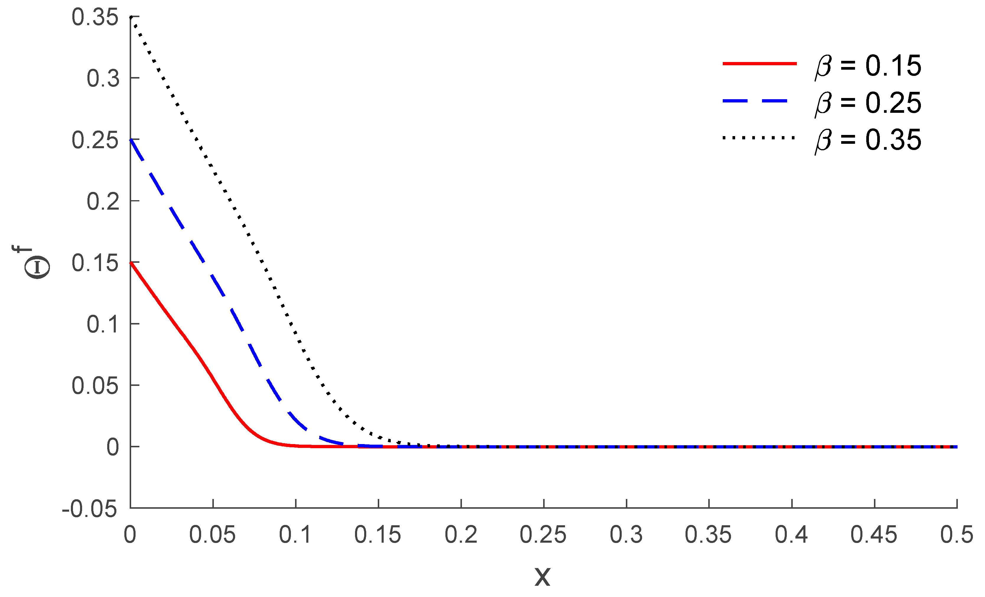
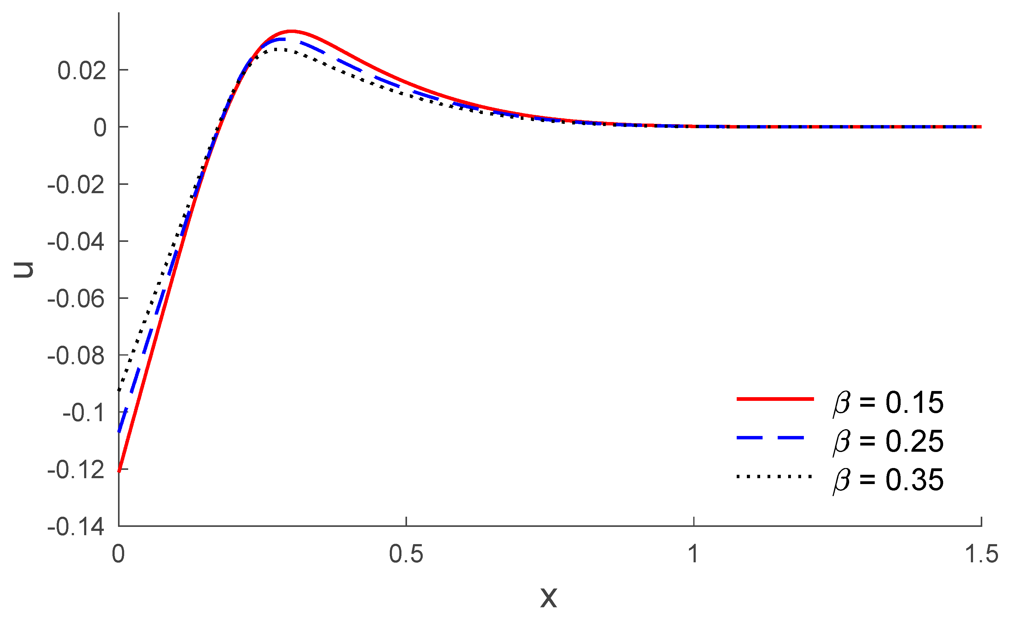
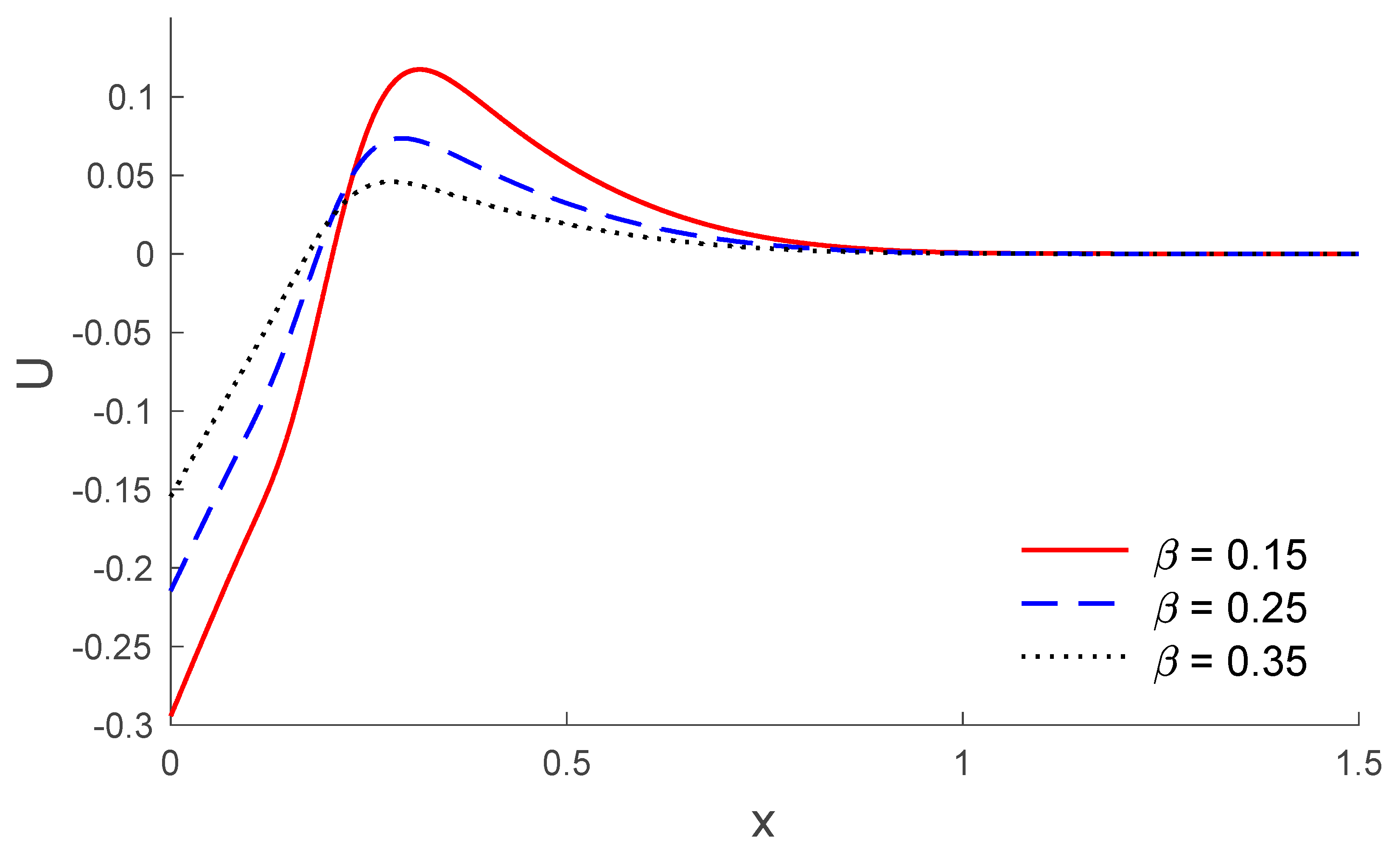
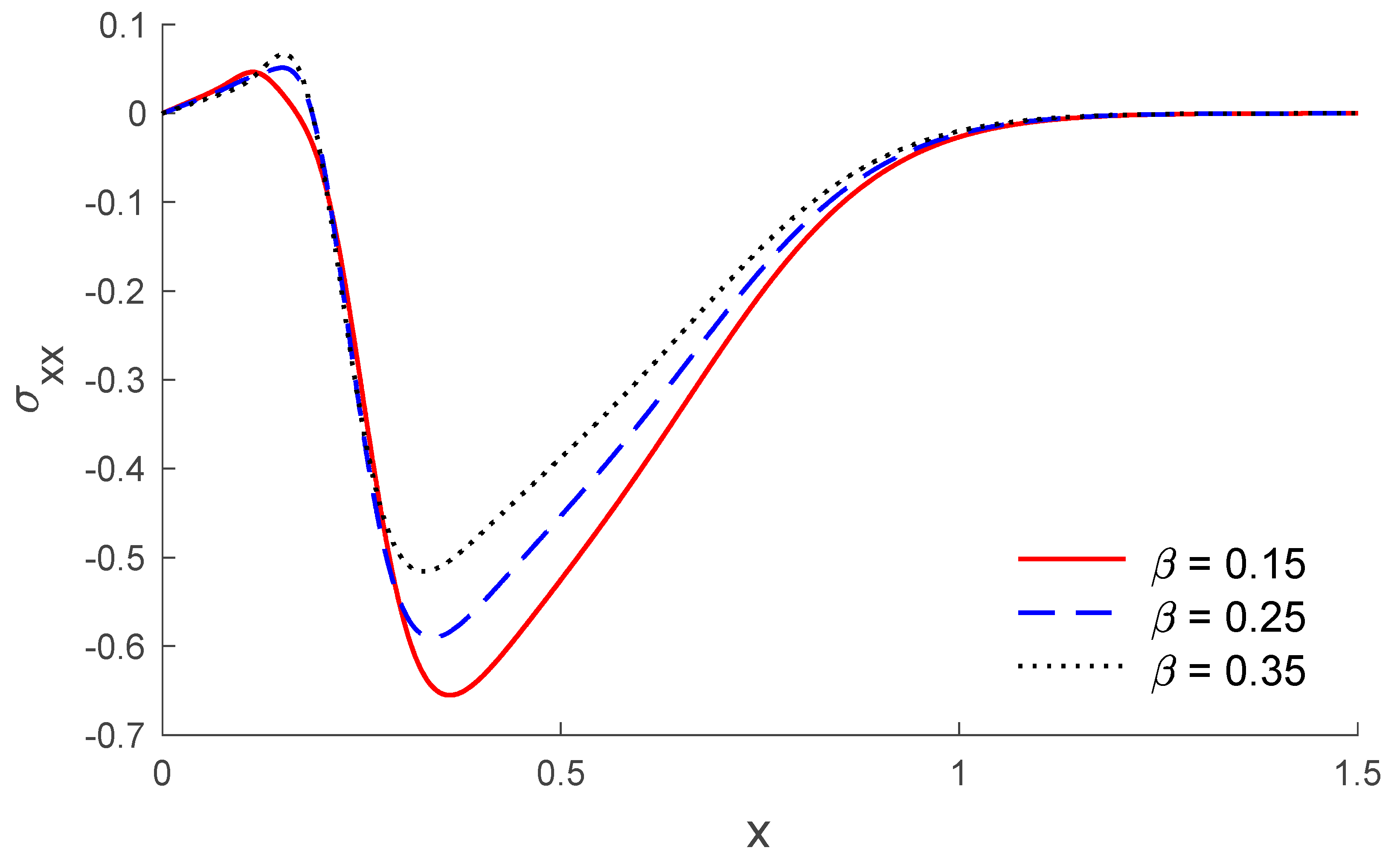
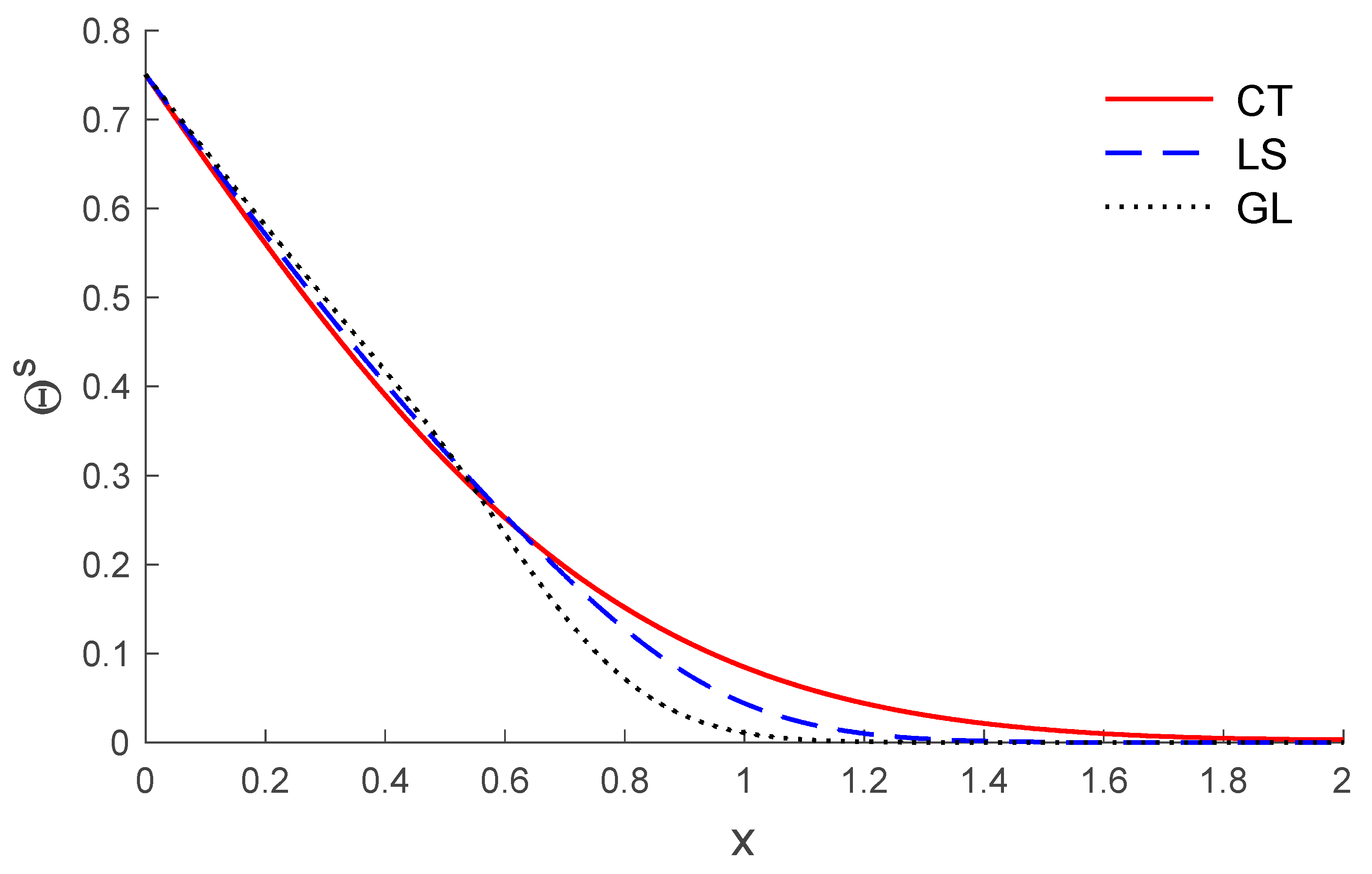
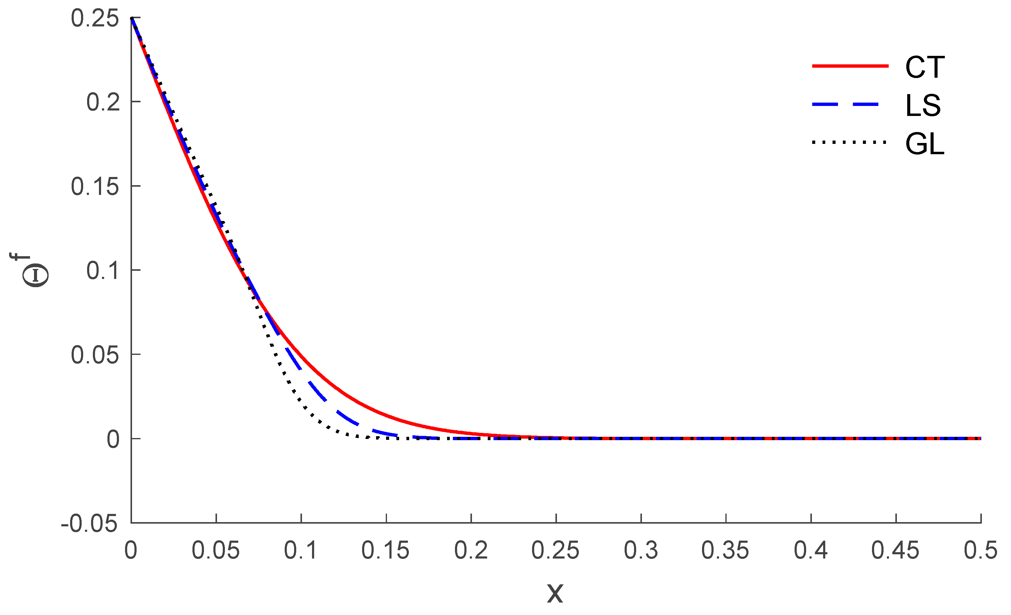
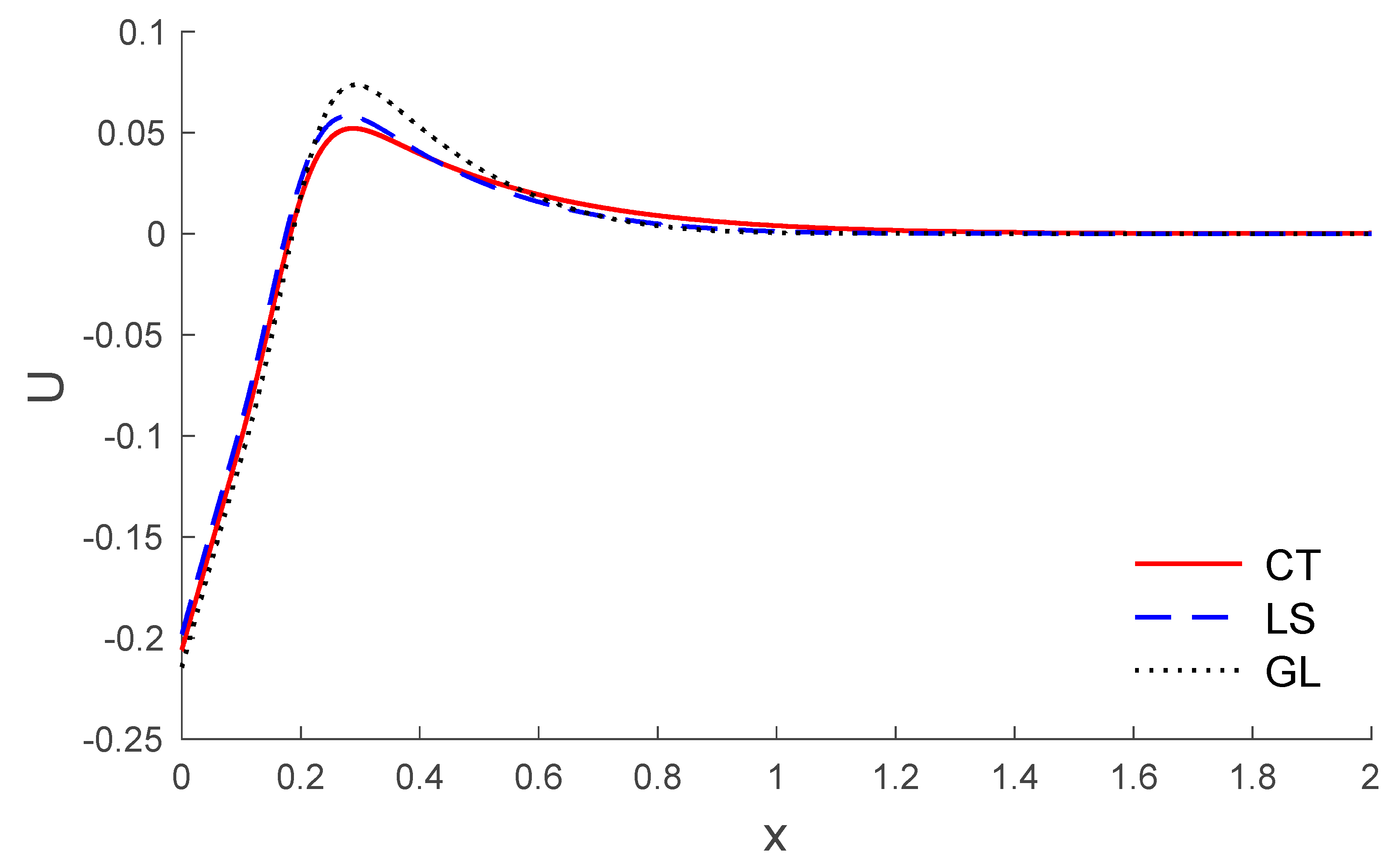
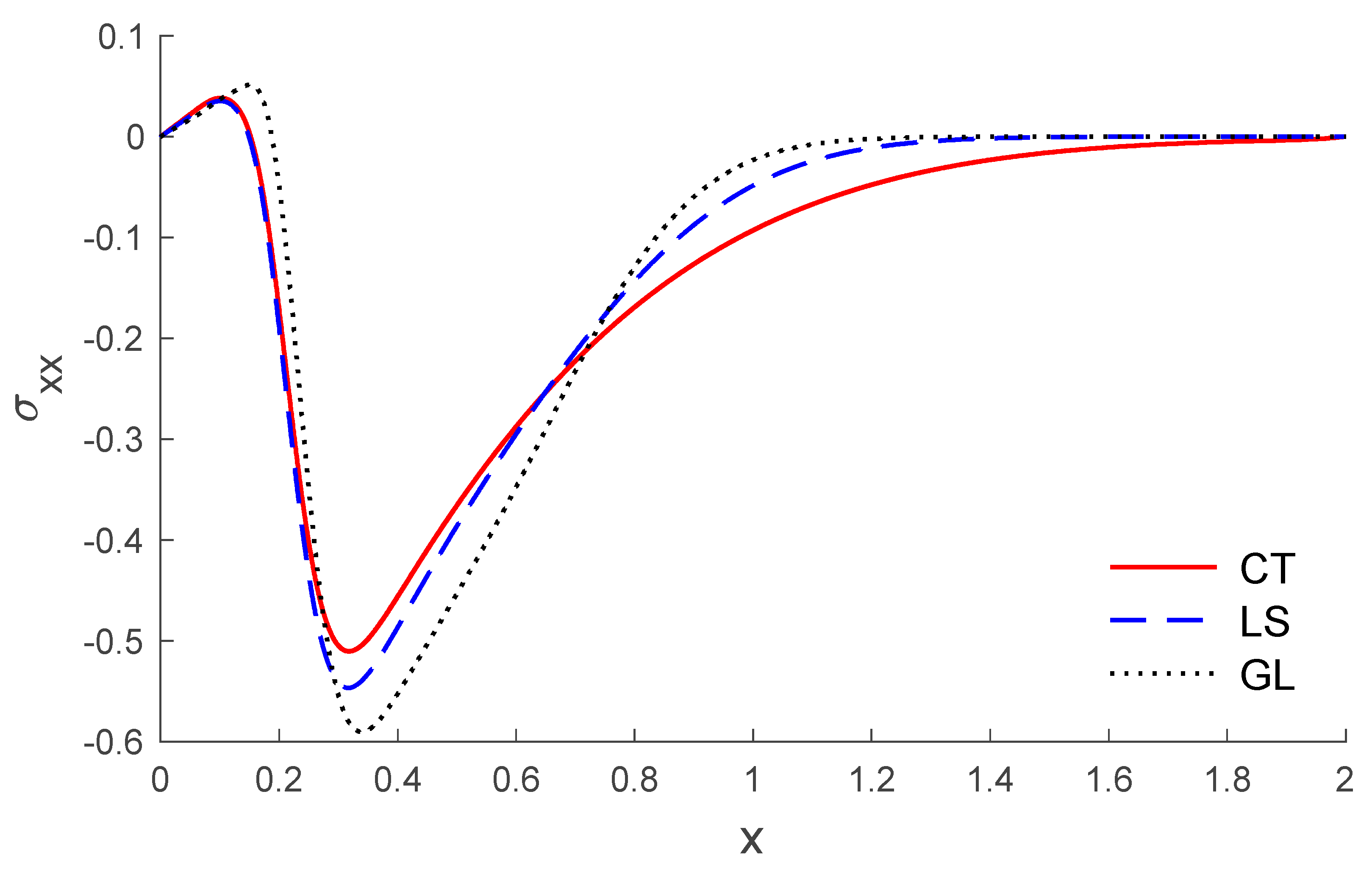
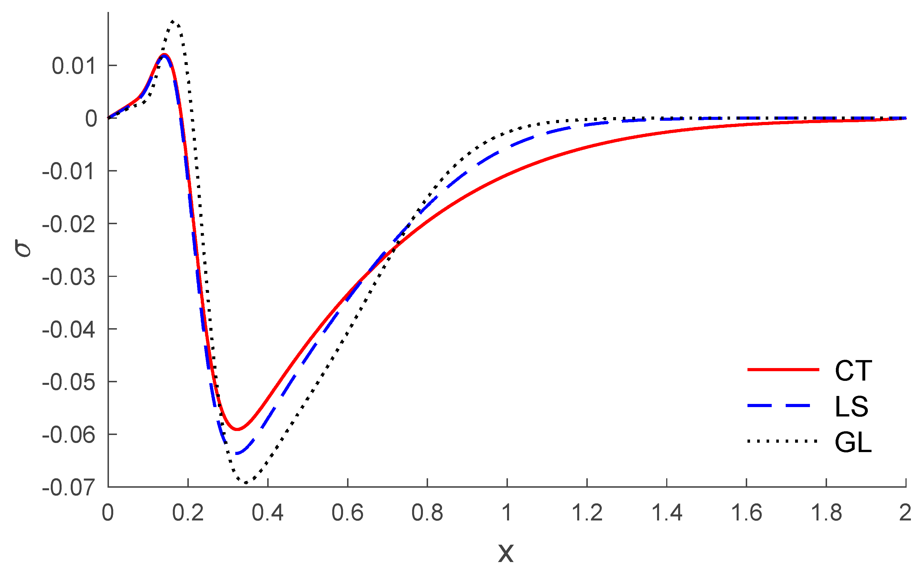
Based on the above dataset, Figure 1, Figure 2, Figure 3, Figure 4, Figure 5, Figure 6, Figure 7, Figure 8, Figure 9, Figure 10, Figure 11 and Figure 12 explain the physical quantities computed numerically at different values of the distance x. Numerical computations are carried out for the solid and liquid temperatures, the displacements and the stresses distributions of solid and liquid phases along the x-axis, in the context of porothermal theory, under four thermal relaxation times. Figure 1, Figure 2, Figure 3, Figure 4, Figure 5 and Figure 6 represent the three curves predicted by various values of porosity considering the time , under Green and Lindsay’s model. Meanwhile, Figure 7, Figure 8, Figure 9, Figure 10, Figure 11 and Figure 12 represent the three curves predicted by various models, considering the time and the porosity . From Figure 1 and Figure 7, it is observed that the temperature of the solid phase starts by its maximum values at and progressively decreases with increases of the distance up to zero, beyond a wave front for the porothermal theory, that satisfies the problem theoretical boundary conditions. Figure 2 and Figure 8 show the variations of the liquid temperature as a function of the distance . It was noted that the values are the highest value on and they decrease when the increasing distance is too close to zero on , which depends on the porosity and the type of model. The displacement changes of solid and liquid phases versus are shown in Figure 3, Figure 4, Figure 9 and Figure 10. It is clear that they attain maximum negative value and increase progressively until they reach maximum values at a particular location near , and then continuously decrease to zero values. Figure 5, Figure 6, Figure 11 and Figure 12 display the effects of the porosity and the thermal relaxation times in the solid and liquid stresses along the distance . As expected, it can be found that the porosity and the thermal relaxation times have major impacts on the values of all the studied fields.
6. Conclusions
Based on the generalized thermoelastic theory with four thermal relaxation times, the variations of temperature, the components of displacement and the components of stress in a poroelastic medium are studied. The non-dimensional resulting has been solved, employing the finite element method. The great effects of the thermal relaxation times and porosity are discussed for all physical quantities. We believe that the analysis of the present study will be useful to understand the basic features of this new model for heat conduction.
Author Contributions
All four authors conceived the framework and structured the whole manuscript, checked the results, and completed the revision of the paper. The authors have equally contributed to the elaboration of this manuscript. All authors have read and approved the final form of the manuscript.
Funding
This project was funded by the Deanship of Scientific Research (DSR) at King Abdulaziz University, Jeddah, Saudi Arabia, under grant no. (KEP-67-130-38). The authors, therefore, acknowledge with thanks DSR technical and financial support.
Conflicts of Interest
The authors declare no conflict of interest.
References
- Biot, M.A. General solutions of the equations of elasticity and consolidation for a porous material. J. Appl. Mech. 1956, 23, 91–96. [Google Scholar]
- Biot, M.A. Theory of propagation of elastic waves in a fluid-saturated porous solid. II. Higher frequency range. J. Acoust. Soc. Am. 1956, 28, 179–191. [Google Scholar] [CrossRef]
- Biot, M.A. Thermoelasticity and irreversible thermodynamics. J. Appl. Phys. 1956, 27, 240–253. [Google Scholar] [CrossRef]
- Lord, H.W.; Shulman, Y. A generalized dynamical theory of thermoelasticity. J. Mech. Phys. Solids 1967, 15, 299–309. [Google Scholar] [CrossRef]
- Green, A.; Lindsay, K. Thermoelasticity. J. Elast. 1972, 2, 1–7. [Google Scholar] [CrossRef]
- McTigue, D. Thermoelastic response of fluid-saturated porous rock. J. Geophys. Res. 1986, 91, 9533–9542. [Google Scholar] [CrossRef]
- Singh, B. On propagation of plane waves in generalized porothermoelasticity. Bull. Seismol. Soc. Am. 2011, 101, 756–762. [Google Scholar] [CrossRef]
- Youssef, H. Theory of generalized porothermoelasticity. Int. J. Rock Mech. Min. Sci. 2007, 44, 222–227. [Google Scholar] [CrossRef]
- Singh, B. Rayleigh surface wave in a porothermoelastic solid half-space. In Proceedings of the Sixth Biot Conference on Poromechanics, Paris, France, 9–13 July 2017; pp. 1706–1713. [Google Scholar]
- Abbas, I. Natural frequencies of a poroelastic hollow cylinder. Acta Mech. 2006, 186, 229–237. [Google Scholar] [CrossRef]
- Schanz, M.; Cheng, A.-D. Transient wave propagation in a one-dimensional poroelastic column. Acta Mech. 2000, 145, 1–18. [Google Scholar] [CrossRef]
- El-Naggar, A.; Kishka, Z.; Abd-Alla, A.; Abbas, I.A.; Abo-Dahab, S.; Elsagheer, M. On the initial stress, magnetic field, voids and rotation effects on plane waves in generalized thermoelasticity. J. Comput. Theor. Nanosci. 2013, 10, 1408–1417. [Google Scholar] [CrossRef]
- Abbas, I.A.; El-Amin, M.; Salama, A. Effect of thermal dispersion on free convection in a fluid saturated porous medium. Int. J. Heat Fluid Flow 2009, 30, 229–236. [Google Scholar] [CrossRef]
- Zenkour, A.M.; Abbas, I.A. A generalized thermoelasticity problem of an annular cylinder with temperature-dependent density and material properties. Int. J. Mech. Sci. 2014, 84, 54–60. [Google Scholar] [CrossRef]
- Abbas, I.A.; Zenkour, A.M. The effect of rotation and initial stress on thermal shock problem for a fiber-reinforced anisotropic half-space using Green-Naghdi theory. J. Comput. Theor. Nanosci. 2014, 11, 331–338. [Google Scholar] [CrossRef]
- Abbas, I.A. The effects of relaxation times and a moving heat source on a two-temperature generalized thermoelastic thin slim strip. Can. J. Phys. 2014, 93, 585–590. [Google Scholar] [CrossRef]
- Abbas, I.A. Nonlinear transient thermal stress analysis of thick-walled FGM cylinder with temperature-dependent material properties. Meccanica 2014, 49, 1697–1708. [Google Scholar] [CrossRef]
- Abbas, I.A. Generalized magneto-thermoelasticity in a nonhomogeneous isotropic hollow cylinder using the finite element method. Arch. Appl. Mech. 2009, 79, 41–50. [Google Scholar] [CrossRef]
- Marin, M.; Öchsner, A. The effect of a dipolar structure on the Hölder stability in Green–Naghdi thermoelasticity. Contin. Mech. Thermodyn. 2017, 29, 1365–1374. [Google Scholar] [CrossRef]
- Sur, A.; Kanoria, M. Memory response on thermal wave propagation in an elastic solid with voids. Mech. Based Des. Struct. Mach. 2019, 1–22. [Google Scholar] [CrossRef]
- Abbas, I.A. Three-phase lag model on thermoelastic interaction in an unbounded fiber-reinforced anisotropic medium with a cylindrical cavity. J. Comput. Theor. Nanosci. 2014, 11, 987–992. [Google Scholar] [CrossRef]
- Sarkar, N.; Mondal, S. Transient responses in a two-temperature thermoelastic infinite medium having cylindrical cavity due to moving heat source with memory-dependent derivative. ZAMM 2019, e201800343. [Google Scholar] [CrossRef]
- Othman, M.I.; Mondal, S. Memory-dependent derivative effect on wave propagation of micropolar thermoelastic medium under pulsed laser heating with three theories. Int. J. Numer. Methods Heat Fluid Flow 2019, 30, 1025–1046. [Google Scholar] [CrossRef]
- Abbas, I.A.; Youssef, H.M. Finite element analysis of two-temperature generalized magneto-thermoelasticity. Arch. Appl. Mech. 2009, 79, 917–925. [Google Scholar] [CrossRef]
- Othman, M.I.; Abbas, I.A. Effect of rotation on plane waves at the free surface of a fibre-reinforced thermoelastic half-space using the finite element method. Meccanica 2011, 46, 413–421. [Google Scholar] [CrossRef]
- Sharma, N.; Kumar, R.; Lata, P. Disturbance due to inclined load in transversely isotropic thermoelastic medium with two temperatures and without energy dissipation. Mater. Phys. Mech. 2015, 22, 107–117. [Google Scholar]
- Sur, A.; Kanoria, M. Thermoelastic interaction in a viscoelastic functionally graded half-space under three-phase-lag model. Eur. J. Comput. Mech. 2014, 23, 179–198. [Google Scholar] [CrossRef]
- Zeeshan, A.; Ellahi, R.; Mabood, F.; Hussain, F. Numerical study on bi-phase coupled stress fluid in the presence of Hafnium and metallic nanoparticles over an inclined plane. Int. J. Numer. Methods Heat Fluid Flow 2019, 29, 2854–2869. [Google Scholar] [CrossRef]
- Sheikholeslami, M.; Ellahi, R.; Shafee, A.; Li, Z. Numerical investigation for second law analysis of ferrofluid inside a porous semi annulus: An application of entropy generation and exergy loss. Int. J. Numer. Methods Heat Fluid Flow 2019, 29, 1079–1102. [Google Scholar] [CrossRef]
- Abbas, I.A.; Kumar, R. Response of thermal source in initially stressed generalized thermoelastic half-space with voids. J. Comput. Theor. Nanosci. 2014, 11, 1472–1479. [Google Scholar] [CrossRef]
- Ellahi, R.; Sait, S.M.; Shehzad, N.; Ayaz, Z. A hybrid investigation on numerical and analytical solutions of electro-magnetohydrodynamics flow of nanofluid through porous media with entropy generation. Int. J. Numer. Methods Heat Fluid Flow 2019, 30, 834–854. [Google Scholar] [CrossRef]
- Milani Shirvan, K.; Mamourian, M.; Mirzakhanlari, S.; Rahimi, A.; Ellahi, R. Numerical study of surface radiation and combined natural convection heat transfer in a solar cavity receiver. Int. J. Numer. Methods Heat Fluid Flow 2017, 27, 2385–2399. [Google Scholar] [CrossRef]
- Milani Shirvan, K.; Mamourian, M.; Ellahi, R. Numerical investigation and optimization of mixed convection in ventilated square cavity filled with nanofluid of different inlet and outlet port. Int. J. Numer. Methods Heat Fluid Flow 2017, 27, 2053–2069. [Google Scholar] [CrossRef]
- Ezzat, M.; Ezzat, S. Fractional thermoelasticity applications for porous asphaltic materials. Pet. Sci. 2016, 13, 550–560. [Google Scholar] [CrossRef] [Green Version]
- Abbas, I.A.; Kumar, R. Deformation due to thermal source in micropolar generalized thermoelastic half-space by finite element method. J. Comput. Theor. Nanosci. 2014, 11, 185–190. [Google Scholar] [CrossRef]
- Mohamed, R.; Abbas, I.A.; Abo-Dahab, S. Finite element analysis of hydromagnetic flow and heat transfer of a heat generation fluid over a surface embedded in a non-Darcian porous medium in the presence of chemical reaction. Commun. Nonlinear Sci. Numer. Simul. 2009, 14, 1385–1395. [Google Scholar] [CrossRef]
- Singh, B. Reflection of plane waves from a free surface of a porothermoelastic solid half-space. J. Porous Media 2013, 16, 945–957. [Google Scholar] [CrossRef]
Figure 1.
The temperature of solid distribution along the distance for different values of porosity.
Figure 1.
The temperature of solid distribution along the distance for different values of porosity.

Figure 2.
The temperature of liquid distribution along the distance for different values of porosity.
Figure 2.
The temperature of liquid distribution along the distance for different values of porosity.

Figure 3.
The displacement of solid distribution along the distance for different values of porosity.
Figure 3.
The displacement of solid distribution along the distance for different values of porosity.

Figure 4.
The displacement of liquid distribution along the distance for different values of porosity.
Figure 4.
The displacement of liquid distribution along the distance for different values of porosity.

Figure 5.
The stress of solid distribution along the distance for different values of porosity.

Figure 6.
The stress of liquid distribution along the distance for different values of porosity.

Figure 7.
The temperature of solid distribution versus the distance for different models.

Figure 8.
The temperature of liquid distribution versus the distance for different models.

Figure 9.
The displacement of solid distribution versus the distance for different models.

Figure 10.
The displacement of liquid distribution versus the distance for different models.

Figure 11.
The stress of solid distribution versus the distance for different models.

Figure 12.
The stress of liquid distribution versus the distance for different models.

© 2020 by the authors. Licensee MDPI, Basel, Switzerland. This article is an open access article distributed under the terms and conditions of the Creative Commons Attribution (CC BY) license (http://creativecommons.org/licenses/by/4.0/).
Share and Cite
MDPI and ACS Style
Saeed, T.; Abbas, I.; Marin, M. A GL Model on Thermo-Elastic Interaction in a Poroelastic Material Using Finite Element Method. Symmetry 2020, 12, 488. https://doi.org/10.3390/sym12030488
AMA Style
Saeed T, Abbas I, Marin M. A GL Model on Thermo-Elastic Interaction in a Poroelastic Material Using Finite Element Method. Symmetry. 2020; 12(3):488. https://doi.org/10.3390/sym12030488
Chicago/Turabian StyleSaeed, Tareq, Ibrahim Abbas, and Marin Marin. 2020. "A GL Model on Thermo-Elastic Interaction in a Poroelastic Material Using Finite Element Method" Symmetry 12, no. 3: 488. https://doi.org/10.3390/sym12030488
Note that from the first issue of 2016, this journal uses article numbers instead of page numbers. See further details here.