Likelihood-Based Inference for the Asymmetric Beta-Skew Alpha-Power Distribution


1
Departamento de Matemáticas y Estadística, Facultad de Ciencias Básicas, Universidad de Córdoba, Montería 230027, Colombia
2
Departamento de Ingeniería Industrial, Facultad de Ciencias e Ingenierías, Universidad del Sinú, Montería 230027, Colombia
*
Author to whom correspondence should be addressed.
Symmetry 2020, 12(4), 613; https://doi.org/10.3390/sym12040613
Submission received: 18 March 2020
/
Revised: 25 March 2020
/
Accepted: 26 March 2020
/
Published: 13 April 2020
(This article belongs to the Special Issue Symmetric and Asymmetric Bimodal Distributions with Applications)
Abstract
:This paper introduces a new family of asymmetric distributions that allows to fit unimodal as well as bimodal and trimodal data sets. The model extends the normal model by introducing two parameters that control the shape and the asymmetry of the distribution. Basic properties of this new distribution are studied in detail. The problem of estimating parameters is addressed by considering the maximum likelihood method and Fisher information matrix is derived. A small Monte Carlo simulation study is conducted to examine the performance of the obtained estimators. Finally, two data set are considered to illustrate the developed methodology.
1. Introduction
Probability distributions for modeling data with high asymmetry and bimodality have been proposed by several authors. They stand out those distributions that have been supported under the general structure of the skew-symmetric probability density function (pdf) given by
where is a symmetric pdf, is an absolutely continuous symmetric cumulative distribution function (cdf) and is a shape parameter. A particular unimodal case of density function given in (1) is the skew-normal (SN) distribution [1], which has pdf given by
where and are the pdf and cdf of the standard normal distribution, respectively. Among the densities of bimodal type supported under general structure (1), it can be stood out the proposals of Arnold et al. [2], Gómez et al. [3] and Kim [4]. Based on the alpha-power family of distributions by Durrans [5] with pdf given by
where is a cdf absolutely continuous, and is a shape parameter, Bolfarine et al. [6] studied a new bimodal distribution. Other proposals for fitting data with bimodal behavior have been considered by Elal-Olivero [7], Elal-Olivero et al. [8] and Ma and Genton [9]. For example, Ma and Genton [9] introduced the family of distributions with pdf
where and are the pdf and cdf of the standard normal distribution, respectively; and is a polynomial of odd order. Elal-Olivero et al. [8] defined the bimodal elliptical skew-normal (BESN) model by multiplying the pdf of the SN distribution by a polynomial of even order resulting the pdf given by
where , is an asymmetry parameter, and is a shape parameter. They showed that the model fits data of bimodal type for . The case is reduced to the SN distribution and for , the standard normal distribution is obtained. An asymmetric extension of the bimodal-normal model which has pdf given by
was proposed by Elal-Olivero [7]. This extension is called the alpha-skew-normal (ASN) distribution and its pdf is
for . This model fits data with bimodal shape for , and for the model is reduced to the normal distribution. Properties of the model and the statistical inference for the parameters can be seen in Elal-Olivero [7]. Recently Shafiei et al. [10] presented a generalization of the ASN model by adding a parameter resulting a more general and flexible model. This addition allows to modeling data sets with the possibility of until four modes and model is denominated alpha-beta skew-normal (ABSN). The pdf of the ABSN model is given by
where . Note that, for the ASN model of Elal-Olivero [7] is obtained, and for the normal distribution is followed.
One of the great disadvantages of the widely known SN model by Azzalini [1], is that the information matrix is singular when . This same characteristic is presented by the BESN model for the case . The bimodal models by Arnold et al. [2] and Gómez et al. [3] also present the problem of singularity of the information matrix. Elal-Olivero [7] shows that ASN distribution has singular information matrix when the shape parameter is equal to zero, and given that ABSN model of Shafiei et al. [10] contains the ASN model as a particular case, it can be shown that for , the ABSN model also has singular information matrix, a situation also presented by the proposal of Ma and Genton [9]. In this way, models of bimodal type that result from including polynomials of even order in the density of normal or skew-normal model; or polynomials of odd order in the argument of skew-normal model, acquire the same characteristic of the skew-normal model in its information matrix; situation that also happens with those models of bimodal type that contain this model as a special case, as it happens with the proposals of Arnold et al. [2] and Gómez et al. [3].
On the other hand, Pewsey et al. [11] studied the alpha-power (AP) model given in (3) for the special case , which is denominated the power-normal (PN) model and they found that values near to one (greater and smaller than one), the information matrix is non-singular, being this an advantage in the inferential process and the asymptotic properties of the maximum likelihood estimator (MLE). Further, Martínez-Flórez et al. [12] extended the SN distribution to the alpha-power family of distributions, and they obtained a more flexible model in terms of asymmetry and kurtosis than SN and PN models. The bimodal model based on the PN distribution of Bolfarine et al. [6] also presents the same property of information matrix non-singular. Hence, given the characteristics of the information matrix of the alpha-power family of distributions, in this paper we propose an extension alpha-power of a multimodal model by using a polynomial of even degree. The introduced model is a more flexible distribution in terms of asymmetry and kurtosis than those existing in the literature and with information matrix non-singular.
The rest of this paper is organized as follows—Section 2 presents the beta-skew alpha-power model and discusses its main properties. In particular, we show how bimodality and trimodality shape are obtained. We consider a location-scale family and the inference process is carried out by using maximum likelihood method. In addition, some properties of the special case of the beta-skew-normal model are studied in details. In Section 3 a small Monte Carlo simulation is presented. In Section 4 two real data application are reported and compares it with several rival models.
2. The Asymmetric Beta-Skew Alpha-Power Distribution
In this section, we introduce a new multimodal asymmetric distribution by considering the asymmetric beta-skew-normal (BSN) model and by incorporating an additional parameter. The new family of distributions extend the usual normal model and others distributions are also particular cases from this model.
Definition 1.
The random variable Z is said to have a beta-skew alpha-power distribution, which we will denote as , if Z has the following pdf
for and . The functions and are the pdf and cdf of the BSN distribution given by
and
respectively. Here, and are de pdf and cdf of the standard normal distribution, respectively.
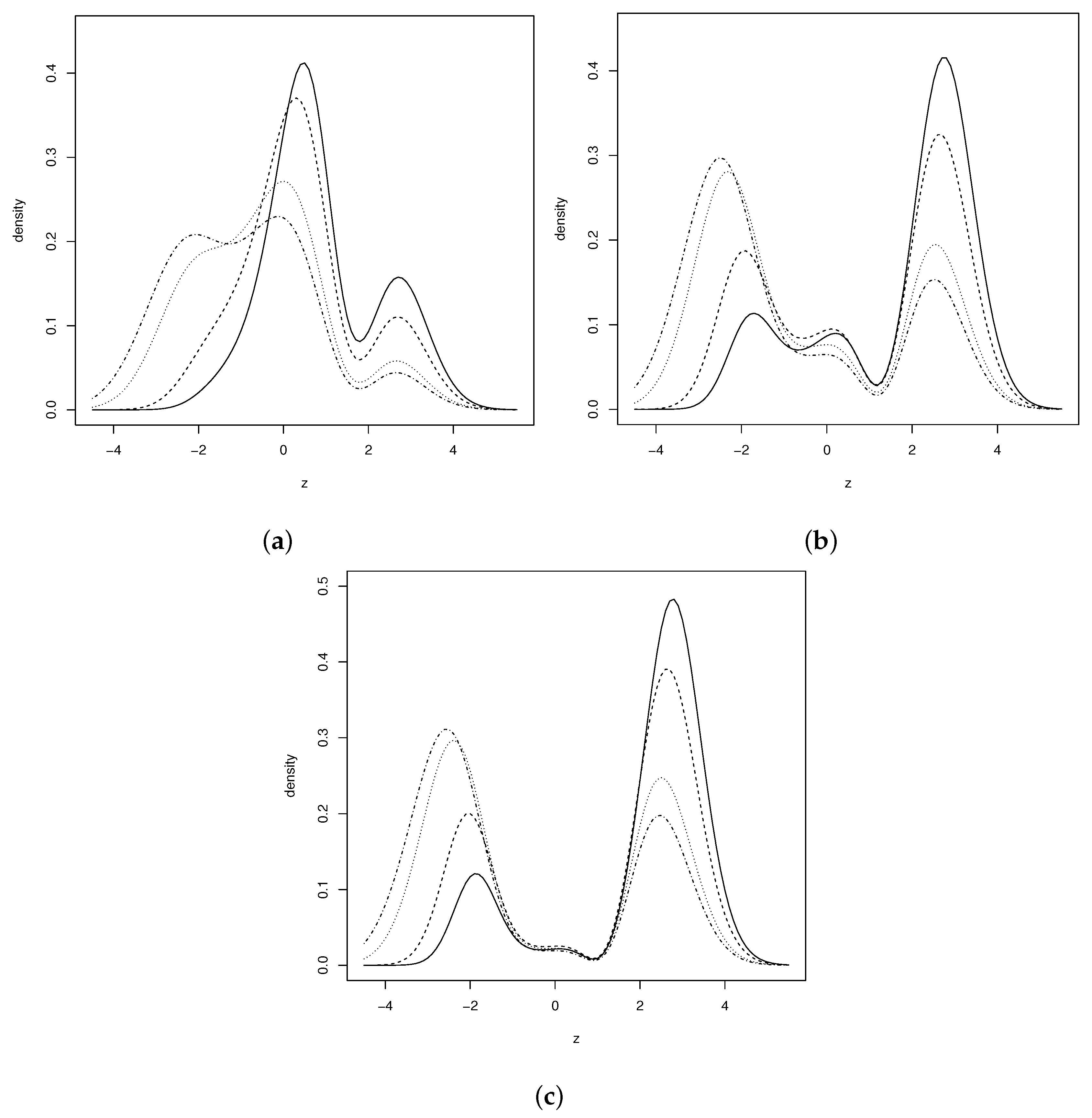
Figure 1 depicts the shape of the beta-skew alpha-power (BSAP) distribution for some selected values of and parameters. It can see from the graph that BSAP distribution has unimodal, bimodal and multimodal (three modes) behavior. Notice that, when increases, the density function takes a bimodal shape. The graphs in the figure also show a bimodal shape for great values of .
If , the following properties are deduced immediately from the definition
- (i)
- If , then .
- (ii)
- If , then .
- (iii)
- If and , then .
Proposition 1.
The density function (9) has at most three modes.
Proof.
Given that is an asymmetry parameter, without loss of generality we take (the case of the BSN distribution) and by differentiating Equation (10) we obtain
thus, has at most seven zeros. It can be seen that for , the value is a zero of the function and it can be shown that , therefore, at occurs a maximum when . By analyzing the polynomial of the BSN model, we making , hence . For the number of positive roots of the polynomial is two, while does not change of sign, hence, the polynomial does not have negative roots. It is concluded that the polynomial has at most four complex roots. For , the polynomial would have two or no negative roots and four complex roots. Using computational methods, it can be shown that for values of the resulting polynomial from the derivative has at least two non-real complex roots, therefore, it would have at most four real roots, and therefore it is concluded that at most they would have three maximums in the model. □
Proposition 2.
Let ,
- (i)
- The cdf of Z, which we denote by , is given by
- (ii)
- The survival function, denoted by , is
- (iii)
- The Hazard function , is
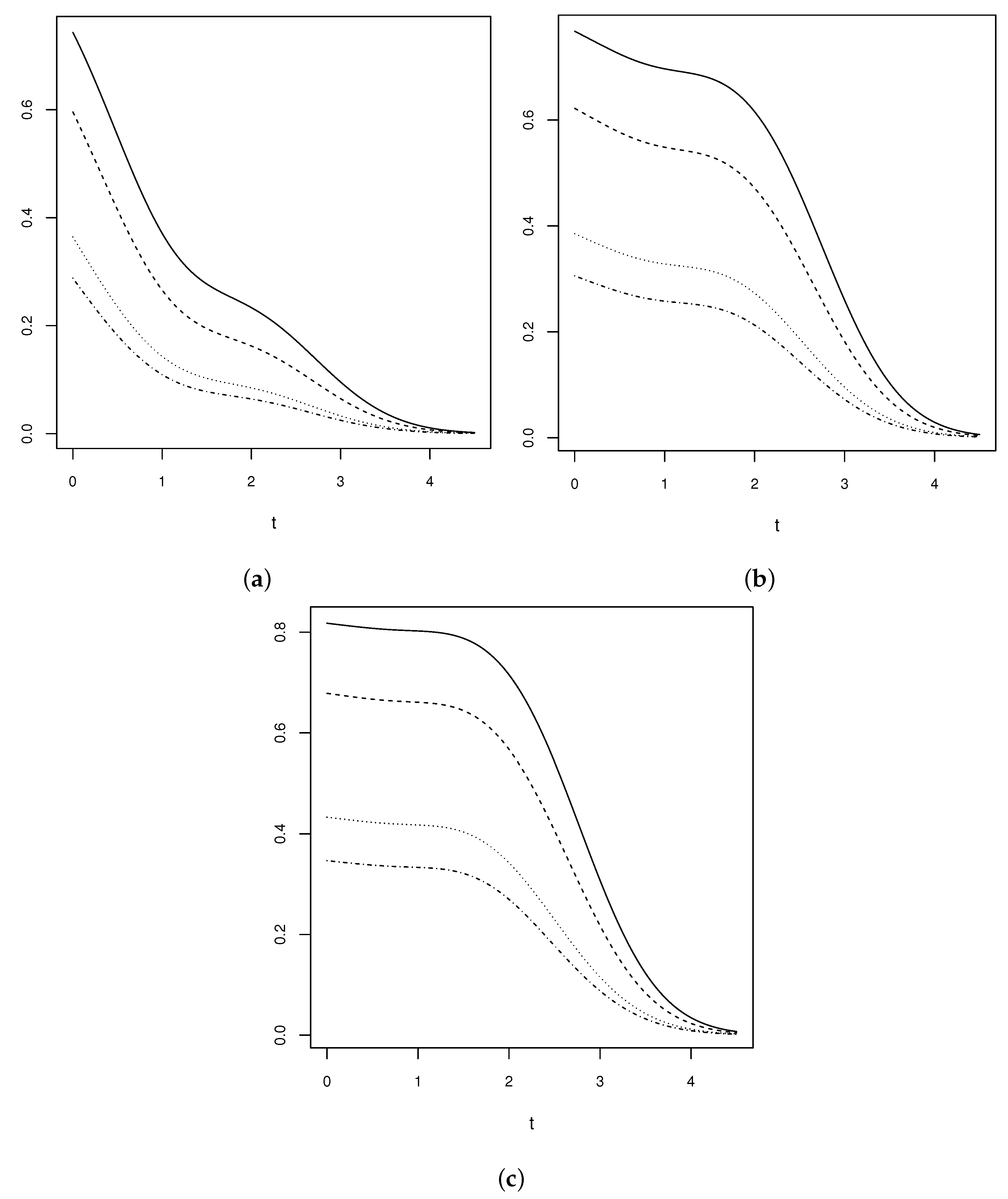
Figure 2 shows the shape of the survival function for some selected values of and . In these graphs, it can be seen that the curve becomes increasingly horizontal in the interval as increases, and the probability of survival is greater for larger values when is constant. It is also important to note that, regardless of the values of and , the survival approaches to zero when z tends to infinite.
Proposition 3.
Let , then the k-th moment of Z is given by
Proof.
The proof is direct from definition of expected value. □
The expected value, the variance and the indices of skewness and kurtosis of the BSAP model, which are denoted by , , and respectively, can be obtained from (16) by using the following expressions
- (i)
- .
- (ii)
- .
- (iii)
- .
- (iv)
- .
Here for .
Remark 1.
We calculated and by using (16) and numerical integration for the model for and . We obtain
Notice that, the length of the admissible intervals for the skewness and the kurtosis parameters of the BSAP distribution are larger than the corresponding intervals of the ASN, the SN, the PN and the skew-normal alpha-power (SNAP) distributions, which are , ; , ; , and , , respectively. See References [1,7,11,12] for more details.
Some additional properties for the special case when are presented to follow.
Lemma 1.
Let , then
Proof.
Knowing that and for when , we obtain
□
Lemma 2.
Let μ, , and the mean, variance and the indices of skewness and kurtosis, respectively of the model,
- (i)
- .
- (ii)
- .
- (iii)
- .
- (iv)
- .
2.1. Location and Scale Extension for BSAP Model
We can also consider a generalization of the distribution by adding location and scale parameters. Next definition gives the generalization of the BSAP model.
Definition 2.
Let . The beta-skew alpha-power density of location and scale is defined as the distribution of , for and . The corresponding density function is given by
where and . We denote this as .
The distribution function associated to the density (20) is given by
and the k-th moment of the random variable X is
where .
2.2. Maximum Likelihood Estimation for BSAP Model
We consider a random sample of size n, from the distribution, where . The log-likelihood function is given by
which is a continuos function in each parameter. Thus, by differentiating the log-likelihood function we obtain the following likelihood equations
where . The solutions of likelihood Equations (21)–(24) provide the maximum likelihood estimators (MLEs) of , , and , which can be obtained by numerical method such as Newton-Rapshon type procedure. Under certain regularity conditions, the elements of the Fisher information may be calculated as
The Cramér–Rao bound states that the inverse of the Fisher information is a lower bound on the variance of any unbiased estimator. Thus, we can find a lower bound for the standard errors (SE) of the MLEs as the square root of the diagonal elements of the observed Fisher information matrix. The observed information matrix can be obtained by taking the second partial derivatives of the log-likelihoiod function and multiplying by −1, that is,
where , , , and . The elements of the expected and observed Fisher information and , respectively, are given in the Appendix A. It can be shown that, for and (the normal distribution case), we have that , therefore, is non-singular. Hence, covariance matrix of the parameter vector is the inverse of the Fisher information matrix, that is, . Thus, the MLE converges to a normal distribution, that is
Remark 2.
The Fisher information matrix for the BSN model is given by
where , for , with , In particular, if then
whose determinant is hence, is non-singular and . Hence, it follows that the MLE converges to the normal distribution
3. Simulation Study
In order to study the performance of the MLEs of the parameters in BSAP model, we conducted a Monte Carlo simulation study with samples sizes , 80, 120, 160 and 320. The true values of the parameters were taken as , 0.5, 2.0 and 5.0; and 1.0, 1.75 and 3.0. For each combination of parameters and sample sizes, we generated 5000 samples from the BSAP model. To evaluate estimators performance were considered the absolute value of the bias (B), and the squared root of the mean squared error (RMSE). They are given by
respectively, where is the estimate of for the j-th sample, for . MLEs were computed by using optim function in R Development Core Team [13].
From Table 1 we can see that, as the sample sizes increase, the bias (in absolute value) and the squared root of the mean squared error decrease, indicating a good behavior of the MLEs of the parameters in BSAP model. Then, it follows that for large sample sizes, MLEs are asymptotically consistent.
4. Real Data Applications
In this section, we illustrate the proposed model by considering two real data sets. In the first application we consider the data on the otis IQ scores of 52 non-white males hired by a large insurance company in 1971. In the second application we use the geyser data set, available in R Development Core Team [13].
4.1. Application 1: The Otis IQ Scores Data
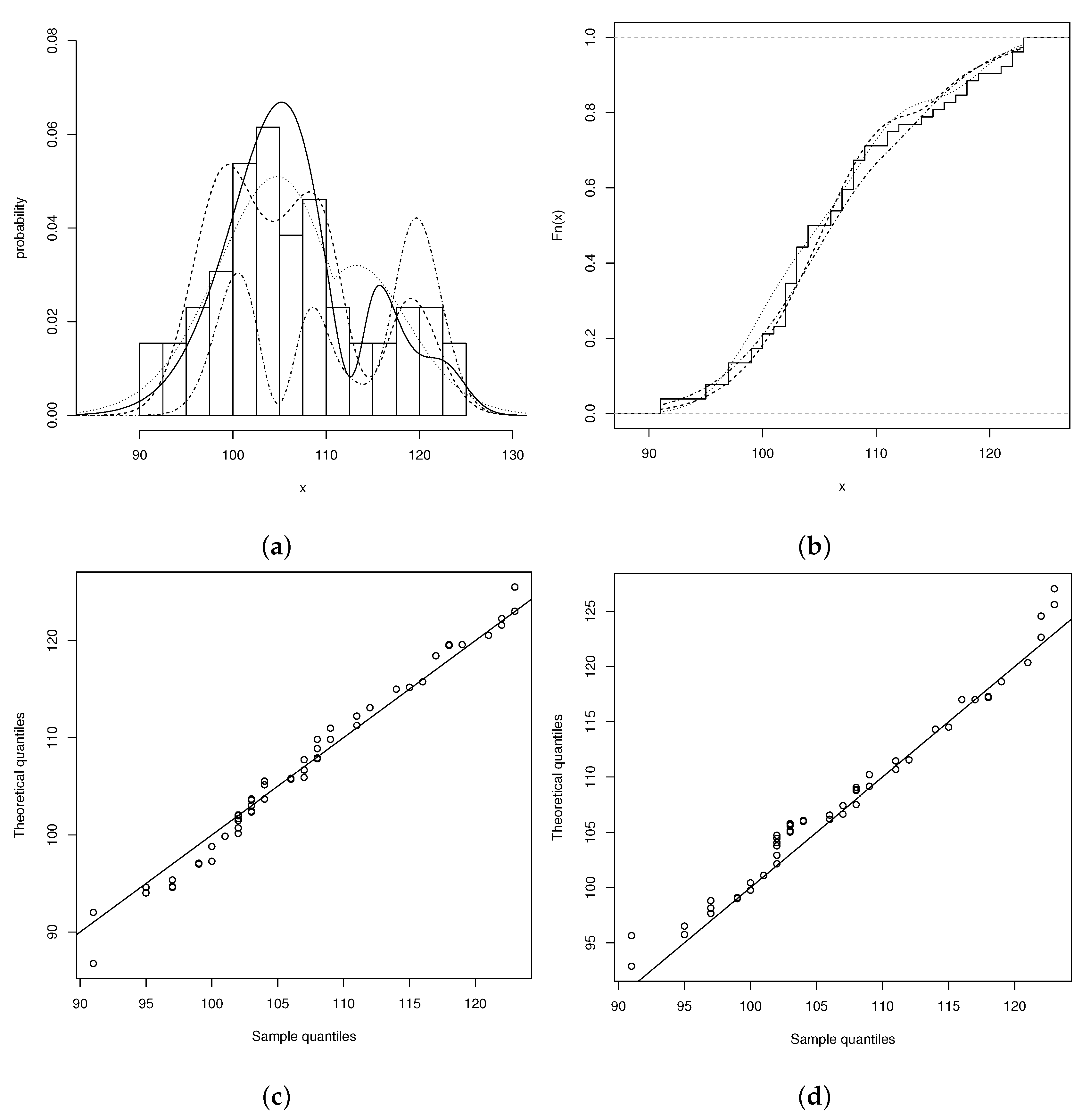
These data set have been analyzed previously by Gupta and Gupta [14] and Sharafi and Behboodian [15]. See, Roberts [16] for more details. Table 2 shows the statistic summary for the otis scores data. The results shows that the data present positives skewness and kurtosis lower than the normal model, likewise, the histogram in Figure 3 shows that the data have more than one mode.
We fit the BSN and BSAP models to analyze this data set. To compare the proposed model, we also fit the multimodal alpha-beta skew-normal (ABSN) model by Shafiei et al. [10], and the asymmetric bimodal model (ETN) of Arnold et al. [2]. The fit of these models is carried out by using the maximum likelihood method and optim function of [13]. Table 3 shows the parameter estimates, together with their corresponding standard errors (SE). To compare fitted models, we use the AIC Akaike [17], corrected CAIC, BIC by Hastie and Tibshirani [18] and the HQIC or information criterion of Hannan and Quinn [19], namely
and
where p is the number of parameters in the considered model. According to any of these criteria, the BSAP and BSN seem to provide better fit to the otis IQ scores data than the ABSN and ETN models.
We can use the likelihood ratio (LR) test statistic to confirm the use the BSAP model instead of the BSN model, so we consider the following hypotheses,
with LR test statistic,
where and denote the likelihood functions of the BSN and BSAP models, respectively. We obtain the value , and comparing this quantity with , the null hypotheses is rejected, that is, the BSAP model is more flexible than the asymmetric BSN model, taking into account the test results of Hartigan and Hartigann [20] and Hartigan [21].
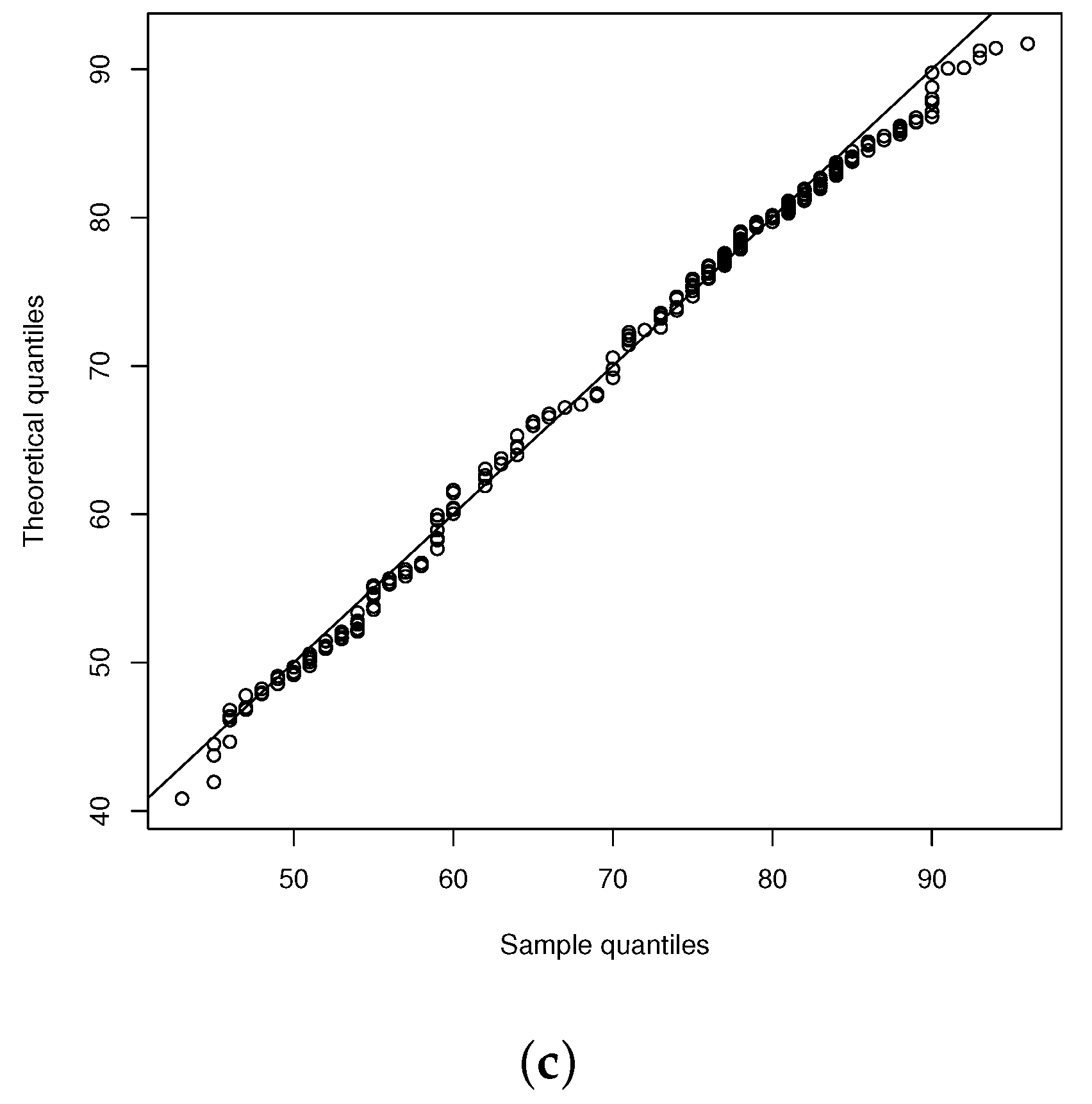
Figure 3a,b show the behavior of the fitted models and the empirical cdf for the ETN, BSN and BSAP models. It can be seen from the figure that the BSAP model has the best fit against the ABSN, BSN and ETN models, while the BSN model has a better fit than the model ETN. Also, the graphs in Figure 3c,d show the QQplots for the BSAP and BSN models.
4.2. Application 2: Old Faithful Geyser Data
For the second application, we consider a data set consisting of 272 observations about the wait times between the eruptions (in minutes) of the old faithful geyser in Yellowstone National Park, Wyoming, U.S. Data set are available in the libraries stats and MASS of R Development Core Team [13]. More information of these data can be seen in Azzalini and Bowman [22] who takes a look at this set of data. Table 4 shows the summary statistic for data set. The results shows that the data set present negative asymmetry and kurtosis below the normal model.
In addition to the BSAP and BSN models, we also fit the ETN and the alpha-skew-normal (ASN) models, see Elal-Olivero [7]. The results of the fit of these models can be seen in Table 5. The standard errors of the estimators were obtained by using the observed information matrix, and again, to compare the fited models, we use the AIC, CAIC, BIC and CAIC criteria. According to any of these criteria, BSAP model seems to provide better fit to the old faithful gayser data than BSN, ASN and ETN models.
We tested the hypotheses
with LR test statistic,
where and denote the likelihood functions of the BSN and BSAP models, respectively. We obtain the value , and comparing this quantity with , the null hypotheses is rejected, that is, the BSAP model is more flexible than the asymmetric BSN model.
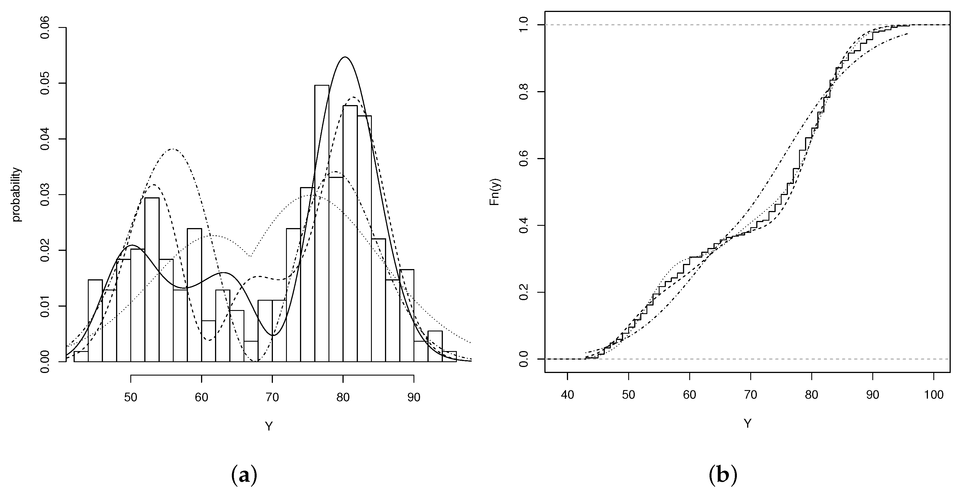
Figure 4 shows the behavior of the fitted models and the empirical cdf for the ETN, BSN and BSAP models. It can be seen that the BSAP model has the best fit against the BSN and ETN models, while the BSN model has a better fit than the ETN model. The graphs in Figure 4 also show the QQplot for the BSAP model.
5. Conclusions
In this paper, a new class of unimodal, as well as bimodal and trimodal, skew distribution was proposed. The main statistical properties of the model and the problem of the parameters estimation are studied in details by using maximum likelihood method. The model extends the usual normal distribution to trimodal asymmetric case and the BSN model is also a special case. Furthermore, we have shown that such distribution is more flexible than certain rival models and it fits better to some real data sets.
Author Contributions
All authors contributed equally to this work. All authors have read and agreed to the published version of the manuscript.
Funding
The research of G. Martínez-Flórez and R. Tovar-Falón was supported by Grant Proyecto Universidad de Córdoba: Familia bimodal de distribuciones de probabilidad skew-normal alpha-potencia, Code FCA-18-15 (Colombia).
Acknowledgments
The authors wish to acknowledge the Associate Editor and two anonymous referees for the constructive comments that helped to improve the quality of the paper.
Conflicts of Interest
The authors declare no conflict of interest.
Appendix A. Information Matrix for the BSAP Model
In this section, expressions for the elements of the observed and expected information matrix of the BSAP model are provided. The observed elements are denoted by , , , , , , , , and , and they can be calculated by using
After some algebraic manipulations we obtain
where
The elements of the expected Fisher information matrix can be obtained by using
and letting
where ; we have
References
- Azzalini, A. A class of distributions which includes the normal ones. Scand. J. Stat. 1985, 12, 171–178. [Google Scholar]
- Arnold, B.C.; Gómez, H.W.; Salinas, H.S. On multiple constraint skewed models. Statistics 2009, 43, 279–293. [Google Scholar] [CrossRef]
- Gómez, H.W.; Elal-Olivero, D.; Salinas, H.S.; Bolfarine, H. Bimodal extension based on the skew-normal distribution with application to pollen data. Environmetrics 2011, 22, 50–62. [Google Scholar] [CrossRef]
- Kim, H.J. On a class of two–piece skew-normal distributions. Statistics 1985, 39, 537–553. [Google Scholar] [CrossRef]
- Durrans, S.R. Distributions of fractional order statistics in hydrology. Water Resour. Res. 1992, 28, 1649–1655. [Google Scholar] [CrossRef]
- Bolfarine, H.; Martínez-Flórez, G.; Salinas, H.S. Bimodal symmetric–asymmetric power–normal families. Commun. Stat. Theory Methods 2018, 47, 259–276. [Google Scholar] [CrossRef]
- Elal-Olivero, D. Alpha-skew-normal distribution. Proyecc. J. Math. 2010, 29, 224–240. [Google Scholar] [CrossRef] [Green Version]
- Elal-Olivero, D.; Gómez, H.W.; Quintana, F.A. Bayesian modeling using a class of bimodal skew–elliptical distributions. J. Stat. Plan. Inference 2010, 139, 1484–1492. [Google Scholar] [CrossRef]
- Ma, Y.; Genton, M.G. Flexible Class of Skew–Symmetric Distributions. Scand. J. Stat. 2004, 31, 459–468. [Google Scholar] [CrossRef] [Green Version]
- Shafiei, S.; Doostparast, M.; Jamalizadeh, A. The alpha–beta skew normal distribution: Properties and applications. Statistics 2016, 50, 338–349. [Google Scholar] [CrossRef]
- Pewsey, A.; Gómez, H.W.; Bolfarine, H. Likelihood–based inference for power distributions. Test 2012, 21, 775–789. [Google Scholar] [CrossRef]
- Martínez-Flórez, G.; Bolfarine, H.; Gómez, H.W. Skew–normal alpha-power model. Statistics 2014, 48, 1414–1428. [Google Scholar] [CrossRef]
- R Development Core Team. R: A Language and Environment for Statistical Computing; R Foundation for Statistical Computing: Vienna, Austria, 2019; Available online: http://www.R-project.org (accessed on 10 December 2019).
- Gupta, R.C.; Gupta, R.D. Generalized skew normal model. Test 2004, 13, 501–524. [Google Scholar] [CrossRef]
- Sharafi, M.; Behboodian, J. The Balakrishnan skew–normal density. Stat. Papers 2008, 49, 769–778. [Google Scholar] [CrossRef]
- Roberts, H. Data Analysis for Managers with MINITAB, 1st ed.; Scientific Press: Redwood City, CA, USA, 1988. [Google Scholar]
- Akaike, H. A new look at statistical model identification. IEEE Trans. Autom. Contr. 1974, 19, 716–722. [Google Scholar] [CrossRef]
- Hastie, T.J.; Tibshirani, R.J. Generalized Additive Models, 1st ed.; Chapman and Hall/CRC: New York, NY, USA, 1990. [Google Scholar]
- Hannan, E.J.; Quinn, B.G. The determination of the order of an autoregression. J. R. Stat. Soc. Ser. B (Stat. Methodol.) 1979, 41, 190–195. [Google Scholar] [CrossRef]
- Hartigan, J.A.; Hartigan, P.M. The dip test of unimodality. Ann. Stat. 1985, 13, 70–84. [Google Scholar] [CrossRef]
- Hartigan, P.M. Algorithm AS 217: Computation of the dip statistic to test for unimodality. J. R. Stat. Soc. Ser. C (Appl. Stat.) 1985, 34, 320–325. [Google Scholar] [CrossRef]
- Azzalini, A.; Bowman, A.W. A look at some data on the old faithful geyser. J. R. Stat. Soc. Ser. C (Appl. Stat.) 1990, 39, 357–365. [Google Scholar] [CrossRef]
Figure 1.
Density function of distribution. (a) for (dotted-dashed line), (dotted line), (dashed line) and (solid line). (b) for (dotted-dashed line), (dotted line), (dashed line) and (solid line). (c) for (dotted-dashed line), (dotted line), (dashed line) and (solid line).
Figure 1.
Density function of distribution. (a) for (dotted-dashed line), (dotted line), (dashed line) and (solid line). (b) for (dotted-dashed line), (dotted line), (dashed line) and (solid line). (c) for (dotted-dashed line), (dotted line), (dashed line) and (solid line).

Figure 2.
Survival function of distribution. (a) for (dotted-dashed line), (dotted line), (dashed line) and (solid line). (b) for (dotted-dashed line), (dotted line), (dashed line) and (solid line). (c) for (dotted-dashed line), (dotted line), (dashed line) and (solid line).
Figure 2.
Survival function of distribution. (a) for (dotted-dashed line), (dotted line), (dashed line) and (solid line). (b) for (dotted-dashed line), (dotted line), (dashed line) and (solid line). (c) for (dotted-dashed line), (dotted line), (dashed line) and (solid line).

Figure 3.
(a) Histogram for the otis data set. BSAP model (solid line), BSN model (dashed line), ETN model (dotted line). (b) Empiric cdf for BSAP model (dashed line), BSN (dotted lines) and ETN model (dotted-dashed line). (c) QQplot for fitted BSAP model. (d) QQplot fitted BSN model.
Figure 3.
(a) Histogram for the otis data set. BSAP model (solid line), BSN model (dashed line), ETN model (dotted line). (b) Empiric cdf for BSAP model (dashed line), BSN (dotted lines) and ETN model (dotted-dashed line). (c) QQplot for fitted BSAP model. (d) QQplot fitted BSN model.

Figure 4.
(a) Histogram for the old faithful geyser data. BSAP model (solid line), BSN model (dotted line), ETN model dashed( line). (b) Empiric cdf for BSAP model (dashed line), BSN (dotted lines) and ETN model (dotted-dashed line). (c) QQplot for fitted BSAP model.
Figure 4.
(a) Histogram for the old faithful geyser data. BSAP model (solid line), BSN model (dotted line), ETN model dashed( line). (b) Empiric cdf for BSAP model (dashed line), BSN (dotted lines) and ETN model (dotted-dashed line). (c) QQplot for fitted BSAP model.


Table 1.
Asymptotic behavior of the MLEsfor the model.
| 0.5 | 1.0 | 40 | 0.0140 | 0.2647 | 0.0120 | 0.0808 | 2.2831 | 6.1943 | 0.0078 | 0.1752 |
| 80 | 0.0105 | 0.1791 | 0.0053 | 0.0580 | 0.6356 | 3.4120 | 0.0061 | 0.1259 | ||
| 120 | 0.0065 | 0.1433 | 0.0040 | 0.0461 | 0.2566 | 2.2942 | 0.0017 | 0.0940 | ||
| 160 | 0.0036 | 0.1212 | 0.0018 | 0.0398 | 0.0996 | 0.7387 | 0.0024 | 0.0803 | ||
| 320 | 0.0010 | 0.0835 | 0.0011 | 0.0270 | 0.0332 | 0.1650 | 0.0014 | 0.0557 | ||
| 1.75 | 40 | 0.0197 | 0.2170 | 0.0093 | 0.0728 | 6.4625 | 9.3573 | 0.0047 | 0.1543 | |
| 80 | 0.0165 | 0.1518 | 0.0064 | 0.0515 | 3.9608 | 8.2540 | 0.0023 | 0.1078 | ||
| 120 | 0.0113 | 0.1270 | 0.0046 | 0.0416 | 2.6714 | 7.6473 | 0.0018 | 0.0884 | ||
| 160 | 0.0097 | 0.1074 | 0.0026 | 0.0355 | 1.6530 | 6.1734 | 0.0001 | 0.0751 | ||
| 320 | 0.0044 | 0.0748 | 0.0014 | 0.0254 | 0.3783 | 2.3064 | 0.0001 | 0.0532 | ||
| 3.0 | 40 | 0.0152 | 0.1938 | 0.0085 | 0.0685 | 9.1202 | 11.7713 | 0.0063 | 0.1449 | |
| 80 | 0.0146 | 0.1371 | 0.0048 | 0.0479 | 8.2167 | 11.0228 | 0.0023 | 0.1007 | ||
| 120 | 0.0125 | 0.1127 | 0.0034 | 0.0389 | 7.6172 | 10.9091 | 0.0024 | 0.0819 | ||
| 160 | 0.0111 | 0.0986 | 0.0029 | 0.0334 | 6.4907 | 10.2152 | 0.0015 | 0.0718 | ||
| 320 | 0.0094 | 0.0709 | 0.0014 | 0.0240 | 3.4155 | 8.9261 | 0.0013 | 0.0504 | ||
| 2.0 | 2.0 | 40 | 0.0192 | 0.2110 | 0.0083 | 0.0615 | 1.1333 | 5.4692 | 0.0195 | 0.4858 |
| 80 | 0.0079 | 0.1414 | 0.0029 | 0.0428 | 0.1469 | 1.3480 | 0.0148 | 0.3384 | ||
| 120 | 0.0070 | 0.1127 | 0.0027 | 0.0340 | 0.0632 | 0.6112 | 0.0044 | 0.2674 | ||
| 160 | 0.0036 | 0.0933 | 0.0012 | 0.0286 | 0.0339 | 0.1686 | 0.0065 | 0.2219 | ||
| 320 | 0.0021 | 0.0667 | 0.0008 | 0.0205 | 0.0171 | 0.1122 | 0.0074 | 0.1594 | ||
| 1.75 | 40 | 0.0239 | 0.1801 | 0.0066 | 0.0523 | 6.4470 | 11.389 | 0.0102 | 0.4745 | |
| 80 | 0.0144 | 0.1276 | 0.0035 | 0.0368 | 2.4806 | 7.4704 | 0.0001 | 0.3290 | ||
| 120 | 0.0084 | 0.1012 | 0.0018 | 0.0288 | 1.3470 | 5.6921 | 0.0077 | 0.2633 | ||
| 160 | 0.0039 | 0.0875 | 0.0011 | 0.0256 | 0.7014 | 4.0847 | 0.0079 | 0.2326 | ||
| 320 | 0.0026 | 0.0589 | 0.0011 | 0.0180 | 0.1161 | 0.6428 | 0.0041 | 0.1546 | ||
| 3.0 | 40 | 0.0171 | 0.1697 | 0.0042 | 0.0506 | 11.8522 | 12.4302 | 0.0224 | 0.4768 | |
| 80 | 0.0151 | 0.1173 | 0.0028 | 0.0341 | 7.8559 | 12.6750 | 0.0085 | 0.3171 | ||
| 120 | 0.0123 | 0.0948 | 0.0031 | 0.0276 | 6.7534 | 11.9330 | 0.0155 | 0.2591 | ||
| 160 | 0.0092 | 0.0860 | 0.0015 | 0.0246 | 5.3014 | 11.2255 | 0.0052 | 0.2308 | ||
| 320 | 0.0053 | 0.0598 | 0.0012 | 0.0172 | 2.2874 | 7.9028 | 0.0073 | 0.1593 | ||
| 5.0 | 1.0 | 40 | 0.0135 | 0.4798 | 0.0023 | 0.1224 | 3.3512 | 8.2619 | 0.8576 | 4.6909 |
| 80 | 0.0070 | 0.2775 | 0.0029 | 0.0743 | 0.9887 | 4.8077 | 0.2170 | 1.7650 | ||
| 120 | 0.0035 | 0.2031 | 0.0036 | 0.0556 | 0.3442 | 2.8067 | 0.1157 | 0.9897 | ||
| 160 | 0.0027 | 0.1646 | 0.0029 | 0.0459 | 0.1134 | 1.1807 | 0.0759 | 0.7488 | ||
| 320 | 0.0027 | 0.1103 | 0.0014 | 0.0308 | 0.0270 | 0.1628 | 0.0398 | 0.4915 | ||
| 1.75 | 40 | 0.0740 | 0.6027 | 0.0108 | 0.1297 | 9.3726 | 10.9680 | 12.947 | 6.5324 | |
| 80 | 0.0118 | 0.3007 | 0.0003 | 0.0712 | 6.8694 | 10.6797 | 0.3210 | 2.4019 | ||
| 120 | 0.0061 | 0.2077 | 0.0018 | 0.0522 | 5.0132 | 10.3183 | 0.1211 | 1.3300 | ||
| 160 | 0.0051 | 0.1609 | 0.0021 | 0.0416 | 3.5124 | 8.9549 | 0.0546 | 0.8401 | ||
| 320 | 0.0024 | 0.1044 | 0.0021 | 0.0278 | 0.9693 | 4.8586 | 0.0151 | 0.5193 | ||
| 3.0 | 40 | 0.1627 | 0.6833 | 0.0280 | 0.1400 | 10.8613 | 12.6877 | 1.9876 | 8.3799 | |
| 80 | 0.0219 | 0.3255 | 0.0019 | 0.0720 | 10.8081 | 11.4270 | 0.4140 | 3.1350 | ||
| 120 | 0.0112 | 0.2030 | 0.0004 | 0.0495 | 9.0012 | 10.9669 | 0.1059 | 1.2182 | ||
| 160 | 0.0060 | 0.1618 | 0.0021 | 0.0403 | 8.5141 | 9.8583 | 0.0573 | 0.9396 | ||
| 320 | 0.0009 | 0.1039 | 0.0023 | 0.0266 | 6.1416 | 8.0937 | 0.0197 | 0.5351 | ||
Table 2.
Statistic summary for the otis IQ scores data.
| Mean | Variance | Skewness | Kurtosis |
|---|---|---|---|
| 106.653 | 8.309 | 0.364 | 2.337 |
Table 3.
Parameter estimates (SE) for the fitted models to the otis IQ scores data.
| Estimate | BSAP | BSN | ABSN | ETN |
|---|---|---|---|---|
| 116.98 (1.010) | 108.210 (0.946) | 110.442 (0.459) | 110.812 (1.336) | |
| 2.764 (0.338) | 4.160 (0.280) | 3.625 (0.187) | 8.48 (0.985) | |
| −0.326 (0.107) | 0.367 (0.076) | 1.225 (0.611) | 1.482 (1.025) | |
| 0.120 (0.040) | −0.828 (0.177) | −0.592 (0.280) | ||
| AIC | 366.97 | 368.99 | 400.74 | 370.92 |
| CAIC | 367.82 | 369.49 | 401.59 | 371.77 |
| BIC | 374.78 | 374.84 | 408.55 | 378.72 |
| HQIC | 369.96 | 371.23 | 403.73 | 373.91 |
Table 4.
Statistic summary for the the old faithful geyser data.
| Mean | Variance | Skewness | Kurtosis |
|---|---|---|---|
| 70.897 | 13.594 | −0.414 | 1.843 |
Table 5.
Parameters estimates(SE) for the fitted models to the old faithful gayser data.
| Estimate | BSAP | BSN | ASN | ETN |
|---|---|---|---|---|
| 61.969 (0.850) | 68.052 (0.376) | 67.228 (0.242) | 66.899 (0.916) | |
| 6.778 (0.231) | 5.836 (0.122) | 8.109 (0.204) | 13.036 (0.589) | |
| 0.672 (0.064) | −0.679 (0.066) | 1.547 (0.336) | ||
| 2.637 (0.267) | 25.111 (8.807) | 0.337 (0.107) | ||
| AIC | 2092.42 | 2099.31 | 2127.04 | 2156.88 |
| CAIC | 2092.56 | 2099.39 | 2127.12 | 2157.02 |
| BIC | 2106.85 | 2110.12 | 2137.86 | 2171.31 |
| HQIC | 2098.21 | 2103.65 | 2131.38 | 2162.67 |
© 2020 by the authors. Licensee MDPI, Basel, Switzerland. This article is an open access article distributed under the terms and conditions of the Creative Commons Attribution (CC BY) license (http://creativecommons.org/licenses/by/4.0/).
Share and Cite
MDPI and ACS Style
Martínez-Flórez, G.; Tovar-Falón, R.; Jimémez-Narváez, M. Likelihood-Based Inference for the Asymmetric Beta-Skew Alpha-Power Distribution. Symmetry 2020, 12, 613. https://doi.org/10.3390/sym12040613
AMA Style
Martínez-Flórez G, Tovar-Falón R, Jimémez-Narváez M. Likelihood-Based Inference for the Asymmetric Beta-Skew Alpha-Power Distribution. Symmetry. 2020; 12(4):613. https://doi.org/10.3390/sym12040613
Chicago/Turabian StyleMartínez-Flórez, Guillermo, Roger Tovar-Falón, and Marvin Jimémez-Narváez. 2020. "Likelihood-Based Inference for the Asymmetric Beta-Skew Alpha-Power Distribution" Symmetry 12, no. 4: 613. https://doi.org/10.3390/sym12040613
Note that from the first issue of 2016, this journal uses article numbers instead of page numbers. See further details here.