Robust Finite-Time Control of Linear System with Non-Differentiable Time-Varying Delay

Abstract

Practical systems such as hybrid power systems are currently implemented around the world. In order to get the system to work properly, the systems usually require their behavior to be maintained or state values to stay within a certain threshold. However, it is difficult to form a perfect mathematical model for describing behavior of the practical systems since there may be some information (uncertainties) that is not observed. Thus, in this article, we studied the stability of an uncertain linear system with a non-differentiable time-varying delay. We constructed Lyapunov-Krasovskii functionals (LKFs) containing several symmetric positive definite matrices to obtain robust finite-time stability (RFTS) and stabilization (RFTU) of the uncertain linear system. With the controller and uncertainties in the considered system, there exist nonlinear terms occurring in the formulation process. Past research handled these nonlinear terms as new variables but this led to some difficulty from a computation point of view. Instead, we applied a novel approach via Cauchy-like matrix inequalities to handle these difficulties. In the end, we present three numerical simulations to show the effectiveness of our proposed theory.

1. Introduction

Many practical systems, such as chemical processes [1], population models [2], atmospheric flow [3,4], spacecraft systems [5], and hydraulic and electric systems [6] are examples of real applications in sciences and engineering fields that commonly possess time delay. It is well known that perfect mathematical models for the practical systems are difficult to form. In practice, mathematical models are only valid under circumstance and may depend upon other unknown complexities or called uncertainties. In fact, these uncertainties are not only significant but also leads to some difficulty of the control design. To improve the models’ efficiency, the uncertainties and delay are crucial factors to be included into the studies of stability problems in control theory. Thus, many stability problems of delay dynamical systems with uncertainties have received more attention from researchers, for example, [5,7,8,9,10].

Past researches on stability are often concerned on systems’ behavior in the long run, for example, asymptotic stability [11] or exponential stability [12,13]. In practical cases, large values of the state variables may be not permissible within a finite time interval. For examples, the temperature or pressure in the industrial processes that should be kept within a specific bound or the reliability of hybrid power system that combines the integrated renewable energy system and the electric power system. The hybrid power system requires the current to be well bounded within the IEEE limits to guarantee efficient operation for real-world usage [6,14]. Thus, it is preferable to investigate the certain bound or behavior of dynamical systems defined over a finite time interval or known as finite-time stability (FTS). In recent decades, the studies of FTS and/or finite-time stabilization (FTU) problems of various systems have been extensively studied because of their practical applications that require norm of the state trajectory to be well bounded within a certain period of time. Some examples of FTS problems are following: FTS on linear systems [15,16,17]; FTU on various systems [18,19,20,21,22,23]; RFTS on various systems [7,9]; RFTU on various systems [5,10,24].

To deal with (R)FTU or RFTS of dynamical systems, the non-linearities usually come into play. Almost all conditions on (R)FTU and RFTS mentioned above except [23], researchers dealt with these nonlinear terms occurring in derivation of stability criteria by defining these nonlinear terms as new variables; e.g., setting $X,Y,Z$ as ${\displaystyle X=P^{-1},Y=P^{-1}Q{P}^{-1}}$ and $Z=P^{-1}R{P}^{-1}$ [17]. However, finding these new variables becomes tricky since these variables relate to one another. Unlike the other, ref. [23] proposed FTU on linear system by applying matrix inequality to deal with these nonlinear terms without defining new variables.

In this research, novel sufficient conditions of RFTU of linear system with time-varying delay and uncertainties are established. The conditions are formulated based on LKFs and written in the forms of inequalities and linear matrix inequalities (LMIs). Instead of defining new variables for nonlinear terms existing in the derivation, we used a new technique, via Cauchy-like matrix inequality, for handling these terms (see Lemma 3). The remainder of this paper is organized as follow. In Section 2, the considered system is introduced along with definitions and lemmas used in the derivation. Section 3, main theorem and corollary are proposed. Section 4, numerical results are given to show the practicable of the proposed conditions and followed by the conclusion.

Notation 1.

Throughout this paper, ${\mathbb{R}}^n$ denotes the n-dimensional space with the scalar product $\langle x,y\rangle =x^{T}y$ and the vector norm $\left|\right|·\left|\right|$. ${\mathbb{R}}^{n\times m}$ represents an $n\times m$ matrix with real entries. $A^T$ denotes the transpose of the matrix A. $\lambda \left(A\right)$ are eigenvalues of A; ${\lambda }_{max}\left(A\right)$ (or ${\lambda }_{min}\left(A\right)$) represents maximum (or minimum) real part of eigenvalue of A. $x_t:=\{x(t+s):s\in [-h_2,0]\}$; $\left|\right|x_t\left|\right|:={sup}_{s\in [-h_2,0]}\left\{\right|\left|x(t+s)\right||,||\dot{x}(t+s)\left|\right|\}$. $A\in {\mathbb{R}}^{n\times n}$ is called semi-positive definite $(A⩾0)$ if $\langle Ax,x\rangle ⩾0$, $\forall x\in {\mathbb{R}}^n$. A is positive definite $(A>0)$ if $\langle Ax,x\rangle >0$, $\forall x\ne 0$. $A>B$ means $A-B>0$. For the sake of simplification, ∗ is used to represent the elements below the main diagonal of a symmetric matrix.

2. Preliminaries

Consider the uncertain linear system with interval time-varying delay of the form:

$$\begin{array}{cc}\hfill \dot{x}\left(t\right)& =(A_0+\Delta A_0\left(t\right))x\left(t\right)+(A_1+\Delta A_1\left(t\right))x(t-h\left(t\right))+(B+\Delta B\left(t\right))u\left(t\right),t\ge 0,\hfill \\ \hfill x\left(t\right)& =\varphi \left(t\right),t\in [-h_2,0],\hfill \end{array}$$

(1)

where $x\left(t\right)\in {\mathbb{R}}^n$ is the state vector. $u\left(t\right)\in {\mathbb{R}}^m$ is the controller. $A_0,A_1\in {\mathbb{R}}^{n\times n}$ and $B\in {\mathbb{R}}^{n\times m}$ are known constant matrices and $h\left(t\right)$ is a continuous function but not necessary to be differentiable satisfying

$$0<h_1\le h\left(t\right)\le h_2,h_1\ne h_2.$$

(2)

$\Delta A_0\left(t\right),\Delta A_1\left(t\right)$ and $\Delta B\left(t\right)$ are parametric structured uncertainties. The uncertainties are assumed to be in the form of

$$[\Delta A_0\left(t\right)\Delta A_1\left(t\right)\Delta B\left(t\right)]=D\Delta \left(t\right)\left[E_0{E}_1{E}_2\right],$$

where $D,E_0,E_1$ and $E_2$ are known real constant matrices with appropriate dimensions; and $\Delta \left(t\right)$ is a norm bounded uncertainty matrix satisfying ${\displaystyle \parallel \Delta \left(t\right)\parallel \le 1}$. The initial condition $\varphi \left(t\right)$ is assumed to be continuous and differentiable vector-valued function for $t\in [-h_2,0]$. To stabilize the system (1), we choose a state-feedback control law of the form [12,21]

$$u\left(t\right)=-\frac{1}{2}{B}^T{P}^{-1}x\left(t\right),$$

(3)

where P is a designed parameter to be determined.

By introducing a new variable ${\displaystyle z\left(t\right)=\Delta \left(t\right)[(E_0-\frac{1}{2}{E}_2{B}^T{P}^{-1})x\left(t\right)+E_{1}x(t-h\left(t\right))]}$, the system (1) can be expressed as following:

$$\begin{array}{cc}\hfill \dot{x}\left(t\right)& =(A_0-\frac{1}{2}B{B}^T{P}^{-1})x\left(t\right)+A_{1}x(t-h\left(t\right))+Dz\left(t\right),t\ge 0,\hfill \\ \hfill x\left(t\right)& =\varphi \left(t\right),t\in [-h_2,0].\hfill \end{array}$$

(4)

To formulate RFTU criteria, the following well-known definition and lemmas are used in this research.

Definition 1

([19]). For given positive numbers $c_1,c_2,T_f$ with $c_1<c_2$ and a symmetric positive definite matrix W, the uncertain control system (1) is robust finite-time stabilizable (RFTU) w.r.t $(c_1,c_2,T_f,h_1,h_2,W)$ if there exists a state feedback controller $u\left(t\right)$ defined in (3) such that

$$\underset{-h_2\le s\le 0}{sup}\left\{x^T\left(s\right)Wx\left(s\right),{\dot{x}}^T\left(s\right)W\dot{x}\left(s\right)\right\}\le c_1\Rightarrow x^T\left(t\right)Wx\left(t\right)<c_2,\forall t\in [0,T_f].$$

(5)

Lemma 1

(Schur complement lemma [21]). Given constant matrices $X,Y,Z$ with appropriate dimensions satisfying $Y=Y^T>0,X=X^T$. Then $X+Z^T{Y}^{-1}Z<0$ if and only if

$$\begin{array}{c}\hfill \left[\begin{array}{cc}X& Z^T\\ Z& -Y\end{array}\right]<0\mathrm{or}\left[\begin{array}{cc}-Y& Z\\ Z^T& X\end{array}\right]<0.\end{array}$$

Lemma 2

([25]). For any symmetric matrix $M\in {\mathbb{R}}^{n\times n}$ and nonsingular $\Pi \in {\mathbb{R}}^{n\times n}$. The matrix M is positive definite if and only if ${\Pi }^{T}M\Pi$ is positive definite. Similarly, M is negative definite matrix if and only if ${\Pi }^{T}M\Pi$ is negative definite.

Lemma 3

(Cauchy-like matrix inequality [23]). For any real matrices Π, $\Sigma \in {\mathbb{R}}^{n\times n}$ with Σ is symmetric positive definite, the following inequality holds

$$-{\Pi }^T{\Sigma }^{-1}\Pi \le -2\Pi +\Sigma .$$

Lemma 4

([23]). For any matrix $R=R^T>0$, scalars $\alpha >0,h_1,h_2,d_1,d_2$ with $0\le h_1\le d_1\le d_2\le h_2$ and $h_{21}=h_2-h_1>0$, the following inequality holds.

$$-{\int }_{t-d_2}^{t-d_1}{e}^{\alpha (t-s)}{\dot{x}}^T\left(s\right)R\dot{x}\left(s\right)ds\le {\left[\begin{array}{c}x(t-d_1)\\ x(t-d_2)\end{array}\right]}^T\left[\begin{array}{cc}-{\mu }_{1}R& {\mu }_{2}R\\ {\mu }_{2}R& -{\mu }_{3}R\end{array}\right]\left[\begin{array}{c}x(t-d_1)\\ x(t-d_2)\end{array}\right]$$

where ${\displaystyle \epsilon =\frac{e^{-\alpha h_1}-e^{-\alpha h_2}}{\alpha },{\mu }_1=2\left(\frac{\alpha }{2}+\frac{1}{h_{21}}\right)e^{\alpha h_1}-\epsilon {\left(\frac{\alpha }{2}+\frac{1}{h_{21}}\right)}^2{e}^{2\alpha h_1},{\mu }_2=\left(\frac{\alpha }{2}+\frac{1}{h_{21}}\right)e^{\alpha h_1}-\left(\frac{\alpha }{2}-\frac{1}{h_{21}}\right)e^{\alpha h_2}+\epsilon \left(\frac{{\alpha }^2}{4}-\frac{1}{h_{21}^2}\right)e^{\alpha (h_1+h_2)},{\mu }_3=-2\left(\frac{\alpha }{2}-\frac{1}{h_{21}}\right)e^{\alpha h_2}-\epsilon {\left(\frac{\alpha }{2}-\frac{1}{h_{21}}\right)}^2{e}^{2\alpha h_2}}$.

Remark 1.

The integral inequality in Lemma 4 only requires one free matrix and used information of ${\left[x^T(t-h_1)x^T(t-h_2)\right]}^T$ in derivation, while the well-known Wirtinger inequality, presented in [11], requires one free matrix but depends on ${\left[x^T(t-h_1)x^T(t-h_2)(1/h_{21}){\int }_{t-h_2}^{t-h_1}{x}^T\left(s\right)ds\right]}^T$. Note that RFTU condition using the Wirtinger inequality is not applicable in our proposed numerical simulation. Thus, in this article, we will only show and discuss results of RFTU conditions of the linear system (1) using Lemma 4.

3. Main Results

In this section, we will derive the RFTU sufficient criteria of the linear system with uncertain and interval time-varying delay as in Equation (1). The derivations of the stability criteria are based on matrix and integral inequalities as stated in lemmas stated in previous section. To derive the main theorem, we first define the following variables for convenient use in the derivation:

$$\begin{array}{cc}\hfill & {\gamma }_1={\displaystyle \frac{e^{\alpha h_1}-1}{\alpha }},{\gamma }_2={\displaystyle \frac{e^{\alpha h_2}-1}{\alpha }},{\gamma }_3={\displaystyle \frac{e^{\alpha h_1}-\alpha h_1-1}{{\alpha }^2}},{\gamma }_4={\displaystyle \frac{e^{\alpha h_2}-e^{\alpha h_1}-\alpha h_{21}}{{\alpha }^2}},{\gamma }_5={\displaystyle \frac{e^{\alpha h_2}-\alpha h_2-1}{{\alpha }^2}},\hfill \\ \hfill & l_1=2\left(\frac{\alpha }{2}+\frac{1}{h_1}\right)-{\epsilon }_1{\left(\frac{\alpha }{2}+\frac{1}{h_1}\right)}^2,l_2=\left(\frac{\alpha }{2}+\frac{1}{h_1}\right)-\left(\frac{\alpha }{2}-\frac{1}{h_1}\right)e^{\alpha h_1}+{\epsilon }_1\left(\frac{{\alpha }^2}{4}-\frac{1}{h_1^2}\right)e^{\alpha h_1},\hfill \\ \hfill & l_3=-2\left(\frac{\alpha }{2}-\frac{1}{h_1}\right)e^{\alpha h_1}-{\epsilon }_1{\left(\frac{\alpha }{2}-\frac{1}{h_1}\right)}^2{e}^{2\alpha h_1},m_1=2\left(\frac{\alpha }{2}+\frac{1}{h_{21}}\right)e^{\alpha h_1}-{\epsilon }_2{\left(\frac{\alpha }{2}+\frac{1}{h_{21}}\right)}^2{e}^{2\alpha h_1},\hfill \\ \hfill & m_2=\left(\frac{\alpha }{2}+\frac{1}{h_{21}}\right)e^{\alpha h_1}-\left(\frac{\alpha }{2}-\frac{1}{h_{21}}\right)e^{\alpha h_2}+{\epsilon }_2\left(\frac{{\alpha }^2}{4}-\frac{1}{h_{21}^2}\right)e^{\alpha (h_1+h_2)},\hfill \\ \hfill & m_3=-2\left(\frac{\alpha }{2}-\frac{1}{h_{21}}\right)e^{\alpha h_2}-{\epsilon }_2{\left(\frac{\alpha }{2}-\frac{1}{h_{21}}\right)}^2{e}^{2\alpha h_2},n_1=2\left(\frac{\alpha }{2}+\frac{1}{h_2}\right)-{\epsilon }_3{\left(\frac{\alpha }{2}+\frac{1}{h_2}\right)}^2,\hfill \\ \hfill & n_2=\left(\frac{\alpha }{2}+\frac{1}{h_2}\right)-\left(\frac{\alpha }{2}-\frac{1}{h_2}\right)e^{\alpha h_2}+{\epsilon }_3\left(\frac{{\alpha }^2}{4}-\frac{1}{h_2^2}\right)e^{\alpha h_2},n_3=-2\left(\frac{\alpha }{2}-\frac{1}{h_2}\right)e^{\alpha h_2}-{\epsilon }_3{\left(\frac{\alpha }{2}-\frac{1}{h_2}\right)}^2{e}^{2\alpha h_2},\hfill \\ \hfill & {\epsilon }_1=\frac{1-e^{-\alpha h_1}}{\alpha }{\epsilon }_2=\frac{e^{-\alpha h_1}-e^{-\alpha h_2}}{\alpha }{\epsilon }_3=\frac{1-e^{-\alpha h_2}}{\alpha }.\hfill \end{array}$$

Now we are ready to formulate the RFTU of the linear system (1) as following.

Theorem 1.

Given $W=W^T>0$. The linear system (1) with time-varying delay $h\left(t\right)$ satisfying (2) is robust finite-time stabilizable with respect to $(c_1,c_2,T_f,h_1,h_2,W),0\le c_1<c_2$, if there exist non-negative scalars $\alpha ,{\beta }_1,{\beta }_2,{\beta }_3,{\beta }_4,{\beta }_5,{\beta }_6$ and ${\beta }_7$, symmetric positive-definite matrices $P,Q_1,Q_2,R_1,R_2,R_3$ and $R_4\in {\mathbb{R}}^{n\times n}$ satisfying

$$\begin{array}{cc}\hfill & {\beta }_{1}I<\tilde{P}<I,{\beta }_{2}I<\widetilde{Q_1},{\beta }_{3}I<\widetilde{Q_2},{\beta }_{4}I<\widetilde{R_1},{\beta }_{5}I<\widetilde{R_2},{\beta }_{6}I<\widetilde{R_3},{\beta }_{7}I<\widetilde{R_4},\hfill \end{array}$$

(6)

$$\chi =\left[\begin{array}{cc}-c_2{e}^{-\alpha T_f}& {\chi }_{12}\\ \ast & -{\chi }_{22},\end{array}\right]<0,$$

(7)

$$\Omega =\left[\begin{array}{cc}\Psi & {\rm Y}\\ \ast & -\Gamma \end{array}\right]<0,$$

(8)

where ${\displaystyle {\chi }_{12}=\left[\sqrt{c_1}\sqrt{c_1{\gamma }_1}\sqrt{c_1{\gamma }_2}\sqrt{c_1{\gamma }_3}\sqrt{c_1{\gamma }_4}\sqrt{c_1{\gamma }_4}\sqrt{c_1{\gamma }_5}\right],{\chi }_{22}=diag({\beta }_1,{\beta }_2,{\beta }_3,{\beta }_4,{\beta }_5,{\beta }_6,{\beta }_7),}$

$$\Psi =\left[\begin{array}{ccccc}{\Psi }_{11}& 0& {\Psi }_{13}& 0& {\Psi }_{15}\\ \ast & {\Psi }_{22}& {\Psi }_{23}& 0& 0\\ \ast & \ast & {\Psi }_{33}& {\Psi }_{34}& 0\\ \ast & \ast & \ast & {\Psi }_{44}& 0\\ \ast & \ast & \ast & \ast & {\Psi }_{55}\end{array}\right],$$

(9)

$$\begin{array}{cc}\hfill & {\Psi }_{11}=A_{0}P+P{A}_0^T-B{B}^T-(\alpha +2l_1+2l_2+2n_1+2n_2)P+(l_1+l_2)R_1+(n_1+n_2)R_4,{\Psi }_{13}=A_1{R}_3,\hfill \\ \hfill & {\Psi }_{15}=D,{\Psi }_{22}=-e^{\alpha h_1}{Q}_1-2(l_2+l_3+2m_1+m_2)Q_1+(l_2+l_3)R_1+(m_1+m_2)R_2+m_1{R}_3,\hfill \\ \hfill & {\Psi }_{23}=m_2{Q}_1,{\Psi }_{33}=-(m_1+m_3)R_3,{\Psi }_{34}=m_2{Q}_2,\hfill \\ \hfill & {\Psi }_{44}=-e^{\alpha h_2}{Q}_2-2(m_2+2m_3+n_2+n_3)Q_2+(m_2+m_3)R_2+m_3{R}_3+(n_2+n_3)R_4,{\Psi }_{55}=-I,\hfill \end{array}$$

$${\rm Y}=\left[\begin{array}{cccccccccc}{{\rm Y}}_{11}& {{\rm Y}}_{12}& {{\rm Y}}_{13}& {{\rm Y}}_{14}& {{\rm Y}}_{15}& 0& {{\rm Y}}_{17}& {{\rm Y}}_{18}& {{\rm Y}}_{19}& {{\rm Y}}_{110}\\ 0& 0& 0& 0& {{\rm Y}}_{25}& {{\rm Y}}_{26}& 0& 0& 0& 0\\ {{\rm Y}}_{31}& {{\rm Y}}_{32}& {{\rm Y}}_{33}& {{\rm Y}}_{34}& 0& 0& 0& 0& 0& {{\rm Y}}_{310}\\ 0& 0& 0& 0& 0& {{\rm Y}}_{46}& {{\rm Y}}_{47}& 0& 0& 0\\ {{\rm Y}}_{51}& {{\rm Y}}_{52}& {{\rm Y}}_{53}& {{\rm Y}}_{54}& 0& 0& 0& 0& 0& 0\end{array}\right],$$

(10)

where

$$\begin{array}{cc}\hfill & {{\rm Y}}_{11}=h_{1}P{A}_0^T-\frac{h_1}{2}B{B}^T,{{\rm Y}}_{12}=h_{21}P{A}_0^T-\frac{h_{21}}{2}B{B}^T,{{\rm Y}}_{13}=h_{21}P{A}_0^T-\frac{h_{21}}{2}B{B}^T,{{\rm Y}}_{14}=h_{2}P{A}_0^T-\frac{h_2}{2}B{B}^T,\hfill \\ \hfill & {{\rm Y}}_{15}=l_{2}P,{{\rm Y}}_{17}=n_{2}P,{{\rm Y}}_{18}=P,{{\rm Y}}_{19}=P,{{\rm Y}}_{110}=P{E}_0^T-\frac{1}{2}B{E}_2^T,{{\rm Y}}_{25}=l_2{Q}_1,{{\rm Y}}_{26}=m_2{Q}_1,\hfill \\ \hfill & {{\rm Y}}_{31}=h_1{R}_3{A}_1^T,{{\rm Y}}_{32}=h_{21}{R}_3{A}_1^T,{{\rm Y}}_{33}=h_{21}{R}_3{A}_1^T,{{\rm Y}}_{34}=h_2{R}_3{A}_1^T,{{\rm Y}}_{310}=R_3{E}_1^T,{{\rm Y}}_{46}=m_2{Q}_2,\hfill \\ \hfill & {{\rm Y}}_{47}=n_2{Q}_2,{{\rm Y}}_{51}=h_1{D}^T,{{\rm Y}}_{52}=h_{21}{D}^T,{{\rm Y}}_{53}=h_{21}{D}^T,{{\rm Y}}_{54}=h_2{D}^T,\hfill \end{array}$$

$$\Gamma =diag(h_1{R}_1,h_{21}{R}_2,h_{21}{R}_3,h_2{R}_4,l_2{R}_1,m_2{R}_2,n_2{R}_4,Q_1,Q_2,I),$$

(11)

and${\displaystyle \tilde{P}=W^{1/2}P{W}^{1/2},\widetilde{Q_i}=W^{1/2}{Q}_i{W}^{1/2},i=1,2,\widetilde{R_j}=W^{1/2}{R}_j{W}^{1/2},j=1,2,3,4.}$

Proof. 

Consider the Lyapunov-Krasovskii functional of the form ${\displaystyle V\left(x\left(t\right)\right)=\sum _{i=1}^7{V}_i\left(x\left(t\right)\right)}$ where

$$\begin{array}{cc}\hfill & V_1\left(x\left(t\right)\right)=x^T\left(t\right)P^{-1}x\left(t\right),\hfill \\ \hfill & V_2\left(x\left(t\right)\right)={\int }_{t-h_1}^t{e}^{\alpha (t-s)}{x}^T\left(s\right)Q_1^{-1}x\left(s\right)ds,\hfill \\ \hfill & V_3\left(x\left(t\right)\right)={\int }_{t-h_2}^t{e}^{\alpha (t-s)}{x}^T\left(s\right)Q_2^{-1}x\left(s\right)ds,\hfill \\ \hfill & V_4\left(x\left(t\right)\right)={\int }_{-h_1}^0{\int }_{t+s}^t{e}^{\alpha (t-\theta )}{\dot{x}}^T\left(\theta \right)R_1^{-1}\dot{x}\left(\theta \right)d\theta ds,\hfill \\ \hfill & V_5\left(x\left(t\right)\right)={\int }_{-h_2}^{-h_1}{\int }_{t+s}^t{e}^{\alpha (t-\theta )}{\dot{x}}^T\left(\theta \right)R_2^{-1}\dot{x}\left(\theta \right)d\theta ds,\hfill \\ \hfill & V_6\left(x\left(t\right)\right)={\int }_{-h_2}^{-h_1}{\int }_{t+s}^t{e}^{\alpha (t-\theta )}{\dot{x}}^T\left(\theta \right)R_3^{-1}\dot{x}\left(\theta \right)d\theta ds,\hfill \\ \hfill & V_7\left(x\left(t\right)\right)={\int }_{-h_2}^0{\int }_{t+s}^t{e}^{\alpha (t-\theta )}{\dot{x}}^T\left(\theta \right)R_4^{-1}\dot{x}\left(\theta \right)d\theta ds.\hfill \end{array}$$

Taking the derivatives of $V\left(x\right(t\left)\right)$ along the Equation (4), we have

$$\begin{array}{cc}\hfill & {\dot{V}}_1\left(x\left(t\right)\right)=x^T\left(t\right)P^{-1}\dot{x}\left(t\right)+{\dot{x}}^T\left(t\right)P^{-1}x\left(t\right),\hfill \\ \hfill & =x^T\left(t\right)P^{-1}{A}_{0}x\left(t\right)+x^T\left(t\right)A_0^T{P}^{-1}x\left(t\right)-x^T\left(t\right)P^{-1}B{B}^T{P}^{-1}x\left(t\right)\hfill \\ \hfill & +2x^T\left(t\right)P^{-1}{A}_{1}x(t-h\left(t\right))+2x^T\left(t\right)P^{-1}Dz\left(t\right)-\alpha x^T\left(t\right)P^{-1}x\left(t\right)+\alpha V_1\left(x\left(t\right)\right),\hfill \\ \hfill & {\dot{V}}_2\left(x\left(t\right)\right)=x^T\left(t\right)Q_1^{-1}x\left(t\right)-e^{\alpha h_1}{x}^T(t-h_1)Q_1^{-1}x(t-h_1)+\alpha V_2\left(x\left(t\right)\right),\hfill \\ \hfill & {\dot{V}}_3\left(x\left(t\right)\right)=x^T\left(t\right)Q_2^{-1}x\left(t\right)-e^{\alpha h_2}{x}^T(t-h_2)Q_2^{-1}x(t-h_2)+\alpha V_3\left(x\left(t\right)\right),\hfill \\ \hfill & {\dot{V}}_4\left(x\left(t\right)\right)=h_1{\dot{x}}^T\left(t\right)R_1^{-1}\dot{x}\left(t\right)-{\int }_{t-h_1}^t{e}^{\alpha (t-s)}{\dot{x}}^T\left(s\right)R_1^{-1}\dot{x}\left(s\right)ds+\alpha V_4\left(x\left(t\right)\right),\hfill \\ \hfill & {\dot{V}}_5\left(x\left(t\right)\right)=h_{21}{\dot{x}}^T\left(t\right)R_2^{-1}\dot{x}\left(t\right)-{\int }_{t-h_2}^{t-h_1}{e}^{\alpha (t-s)}{\dot{x}}^T\left(s\right)R_2^{-1}\dot{x}\left(s\right)ds+\alpha V_5\left(x\left(t\right)\right),\hfill \\ \hfill & {\dot{V}}_6\left(x\left(t\right)\right)=h_{21}{\dot{x}}^T\left(t\right)R_3^{-1}\dot{x}\left(t\right)-{\int }_{t-h_2}^{t-h_1}{e}^{\alpha (t-s)}{\dot{x}}^T\left(s\right)R_3^{-1}\dot{x}\left(s\right)ds+\alpha V_6\left(x\left(t\right)\right),\hfill \\ \hfill & {\dot{V}}_7\left(x\left(t\right)\right)=h_2{\dot{x}}^T\left(t\right)R_4^{-1}\dot{x}\left(t\right)-{\int }_{t-h_2}^t{e}^{\alpha (t-s)}{\dot{x}}^T\left(s\right)R_4^{-1}\dot{x}\left(s\right)ds+\alpha V_7\left(x\left(t\right)\right).\hfill \end{array}$$

Define $\eta \left(t\right)={\left[x^T\left(t\right)x^T(t-h_1)x^T(t-h\left(t\right))x^T(t-h_2)z^T\left(t\right)\right]}^T$. We have

$${[(E_0-\frac{1}{2}{E}_2{B}^T{P}^{-1})x\left(t\right)+E_{1}x(t-h\left(t\right))]}^T[(E_0-\frac{1}{2}{E}_2{B}^T{P}^{-1})x\left(t\right)+E_{1}x(t-h\left(t\right))]-z^T\left(t\right)z\left(t\right)\ge 0.$$

This leads to

$$\begin{array}{cc}\hfill & {\eta }^T\left(t\right)\left[\begin{array}{c}{(E_0-\frac{1}{2}{E}_2{B}^T{P}^{-1})}^T\\ 0\\ E_1^T\\ 0\\ 0\end{array}\right]I{\left[\begin{array}{c}{(E_0-\frac{1}{2}{E}_2{B}^T{P}^{-1})}^T\\ 0\\ E_1^T\\ 0\\ 0\end{array}\right]}^T\eta \left(t\right)+{\eta }^T\left(t\right)\left[\begin{array}{ccccc}0& 0& 0& 0& 0\\ 0& 0& 0& 0& 0\\ 0& 0& 0& 0& 0\\ 0& 0& 0& 0& 0\\ 0& 0& 0& 0& -I\end{array}\right]\eta \left(t\right)\ge 0.\hfill \end{array}$$

(12)

Combining the derivatives of ${\displaystyle V_i\left(x\left(t\right)\right)}$ and applying relations (4) and (12), we obtain

$$\begin{array}{cc}\hfill & \dot{V}\left(x\left(t\right)\right)-\alpha V\left(x\left(t\right)\right)\le {\eta }^T\left(t\right)\left[\begin{array}{ccccc}{\Theta }_{11}& 0& P^{-1}{A}_1& 0& P^{-1}D\\ 0& -e^{\alpha h_1}{Q}_1^{-1}& 0& 0& 0\\ A_1^T{P}^{-1}& 0& 0& 0& 0\\ 0& 0& 0& -e^{\alpha h_2}{Q}_2^{-1}& 0\\ D^T{P}^{-1}& 0& 0& 0& -I\end{array}\right]\eta \left(t\right)\hfill \\ \hfill & +h_1{\eta }^T\left(t\right){\left[\begin{array}{c}(A_0-\frac{1}{2}B{B}^T{P}^{-1})0A_{1}0D\end{array}\right]}^T{R}_1^{-1}\left[\begin{array}{c}(A_0-\frac{1}{2}B{B}^T{P}^{-1})0A_{1}0D\end{array}\right]\eta \left(t\right)\hfill \\ \hfill & +h_{21}{\eta }^T\left(t\right){\left[\begin{array}{c}(A_0-\frac{1}{2}B{B}^T{P}^{-1})0A_{1}0D\end{array}\right]}^T{R}_2^{-1}\left[\begin{array}{c}(A_0-\frac{1}{2}B{B}^T{P}^{-1})0A_{1}0D\end{array}\right]\eta \left(t\right)\hfill \\ \hfill & +h_{21}{\eta }^T\left(t\right){\left[\begin{array}{c}(A_0-\frac{1}{2}B{B}^T{P}^{-1})0A_{1}0D\end{array}\right]}^T{R}_3^{-1}\left[\begin{array}{c}(A_0-\frac{1}{2}B{B}^T{P}^{-1})0A_{1}0D\end{array}\right]\eta \left(t\right)\hfill \\ \hfill & +h_2{\eta }^T\left(t\right){\left[\begin{array}{c}(A_0-\frac{1}{2}B{B}^T{P}^{-1})0A_{1}0D\end{array}\right]}^T{R}_4^{-1}\left[\begin{array}{c}(A_0-\frac{1}{2}B{B}^T{P}^{-1})0A_{1}0D\end{array}\right]\eta \left(t\right)\hfill \\ \hfill & +{\eta }^T\left(t\right){\left[\begin{array}{c}(E_0-\frac{1}{2}{E}_2{B}^T{P}^{-1})0E_{1}00\end{array}\right]}^{T}I\left[\begin{array}{c}(E_0-\frac{1}{2}{E}_2{B}^T{P}^{-1})0E_{1}00\end{array}\right]\eta \left(t\right)\hfill \\ \hfill & -{\int }_{t-h_1}^t{e}^{\alpha (t-s)}{\dot{x}}^T\left(s\right)R_1^{-1}\dot{x}\left(s\right)ds-{\int }_{t-h_2}^{t-h_1}{e}^{\alpha (t-s)}{\dot{x}}^T\left(s\right)R_2^{-1}\dot{x}\left(s\right)ds\hfill \end{array}$$

$$-{\int }_{t-h_2}^{t-h_1}{e}^{\alpha (t-s)}{\dot{x}}^T\left(s\right)R_3^{-1}\dot{x}\left(s\right)ds-{\int }_{t-h_2}^t{e}^{\alpha (t-s)}{\dot{x}}^T\left(s\right)R_4^{-1}\dot{x}\left(s\right)ds,$$

(13)

where ${\Theta }_{11}=P^{-1}{A}_0+A_0^T{P}^{-1}+Q_1^{-1}+Q_2^{-1}-P^{-1}B{B}^T{P}^{-1}-\alpha P^{-1}$.

Applying Lemma 4 for the integral terms in the inequality (13), we have

$$\begin{array}{cc}\hfill & -{\int }_{t-h_1}^t{e}^{\alpha (t-s)}{\dot{x}}^T\left(s\right)R_1^{-1}\dot{x}\left(s\right)ds\le {\eta }^T\left(t\right){\Theta }_1\eta \left(t\right),\hfill \end{array}$$

(14)

$$\begin{array}{c}-{\int }_{t-h_2}^{t-h_1}{e}^{\alpha (t-s)}{\dot{x}}^T\left(s\right)R_2^{-1}\dot{x}\left(s\right)ds\le {\eta }^T\left(t\right){\Theta }_2\eta \left(t\right),\hfill \end{array}$$

(15)

$$\begin{array}{cc}\hfill -{\int }_{t-h_2}^{t-h_1}{e}^{\alpha (t-s)}{\dot{x}}^T\left(s\right)R_3^{-1}\dot{x}\left(s\right)ds& =-{\int }_{t-h\left(t\right)}^{t-h_1}{e}^{\alpha (t-s)}{\dot{x}}^T\left(s\right)R_3^{-1}\dot{x}\left(s\right)ds-{\int }_{t-h_2}^{t-h\left(t\right)}{e}^{\alpha (t-s)}{\dot{x}}^T\left(s\right)R_3^{-1}\dot{x}\left(s\right)ds,\hfill \\ & \le {\eta }^T\left(t\right)\left({\Theta }_3+{\Theta }_4\right)\eta \left(t\right),\hfill \end{array}$$

(16)

$$\begin{array}{cc}\hfill & -{\int }_{t-h_2}^t{e}^{\alpha (t-s)}{\dot{x}}^T\left(s\right)R_4^{-1}\dot{x}\left(s\right)ds\le {\eta }^T\left(t\right){\Theta }_5\eta \left(t\right),\hfill \end{array}$$

(17)

where

$$\begin{array}{cc}\hfill & {\Theta }_1=\left[\begin{array}{ccccc}-l_1{R}_1^{-1}& l_2{R}_1^{-1}& 0& 0& 0\\ l_2{R}_1^{-1}& -l_3{R}_1^{-1}& 0& 0& 0\\ 0& 0& 0& 0& 0\\ 0& 0& 0& 0& 0\\ 0& 0& 0& 0& 0\end{array}\right],{\Theta }_2=\left[\begin{array}{ccccc}0& 0& 0& 0& 0\\ 0& -m_1{R}_2^{-1}& 0& m_2{R}_2^{-1}& 0\\ 0& 0& 0& 0& 0\\ 0& m_2{R}_2^{-1}& 0& -m_3{R}_2^{-1}& 0\\ 0& 0& 0& 0& 0\end{array}\right],\hfill \\ \hfill & {\Theta }_3=\left[\begin{array}{ccccc}0& 0& 0& 0& 0\\ 0& -m_1{R}_3^{-1}& m_2{R}_3^{-1}& 0& 0\\ 0& m_2{R}_3^{-1}& -m_3{R}_3^{-1}0& & 0\\ 0& 0& 0& 0& 0\\ 0& 0& 0& 0& 0\end{array}\right],{\Theta }_4=\left[\begin{array}{ccccc}0& 0& 0& 0& 0\\ 0& 0& 0& 0& 0\\ 0& 0& -m_1{R}_3^{-1}& m_2{R}_3^{-1}& 0\\ 0& 0& m_2{R}_3^{-1}& -m_3{R}_3^{-1}& 0\\ 0& 0& 0& 0& 0\end{array}\right],\hfill \\ \hfill & {\Theta }_5=\left[\begin{array}{ccccc}-n_1{R}_4^{-1}& 0& 0& n_2{R}_4^{-1}& 0\\ 0& 0& 0& 0& 0\\ 0& 0& 0& 0& 0\\ n_2{R}_4^{-1}& 0& 0& -n_3{R}_4^{-1}& 0\\ 0& 0& 0& 0& 0\end{array}\right].\hfill \end{array}$$

Substituting inequalities (14)–(17) into (13) and rearranging these terms, we obtain

$$\dot{V}\left(x\left(t\right)\right)-\alpha V\left(x\left(t\right)\right)\le {\eta }^T\left(t\right)M\eta \left(t\right),$$

(18)

where

$$\begin{array}{c}M=\Sigma +{\left[\begin{array}{c}(A_0-\frac{1}{2}B{B}^T{P}^{-1})0A_{1}0D\end{array}\right]}^T\left(h_1{R}_1^{-1}+h_{21}{R}_2^{-1}+h_{21}{R}_3^{-1}+h_2{R}_4^{-1}\right)\left[\begin{array}{c}(A_0-\frac{1}{2}B{B}^T{P}^{-1})0A_{1}0D\end{array}\right]\hfill \\ +{\left[\begin{array}{c}(E_0-\frac{1}{2}{E}_2{B}^T{P}^{-1})0E_{1}00\end{array}\right]}^{T}I\left[\begin{array}{c}(E_0-\frac{1}{2}{E}_2{B}^T{P}^{-1})0E_{1}00\end{array}\right],\hfill \end{array}$$

(19)

$$\Sigma =\left[\begin{array}{ccccc}{\Sigma }_{11}& {\Sigma }_{12}& {\Sigma }_{13}& {\Sigma }_{14}& {\Sigma }_{15}\\ \ast & {\Sigma }_{22}& {\Sigma }_{23}& {\Sigma }_{24}& 0\\ \ast & \ast & {\Sigma }_{33}& {\Sigma }_{34}& 0\\ \ast & \ast & \ast & {\Sigma }_{44}& 0\\ \ast & \ast & \ast & \ast & {\Sigma }_{55}\end{array}\right],$$

(20)

$$\begin{array}{cc}\hfill & {\Sigma }_{11}=P^{-1}{A}_0+A_0^T{P}^{-1}+Q_1^{-1}+Q_2^{-1}-P^{-1}B{B}^T{P}^{-1}-\alpha P^{-1}-l_1{R}_1^{-1}-n_1{R}_4^{-1},{\Sigma }_{12}=l_2{R}_1^{-1},\hfill \\ \hfill & {\Sigma }_{13}=P^{-1}{A}_1,{\Sigma }_{14}=n_2{R}_4^{-1},{\Sigma }_{15}=P^{-1}D,{\Sigma }_{22}=-e^{\alpha h_1}{Q}_1^{-1}-l_3{R}_1^{-1}-m_1{R}_2^{-1}-m_1{R}_3^{-1},\hfill \\ \hfill & {\Sigma }_{23}=m_2{R}_3^{-1},{\Sigma }_{24}=m_2{R}_2^{-1},{\Sigma }_{33}=-(m_1+m_3)R_3^{-1},{\Sigma }_{34}=m_2{R}_3^{-1},\hfill \\ \hfill & {\Sigma }_{44}=-e^{\alpha h_2}{Q}_2^{-1}-m_3{R}_2^{-1}-m_3{R}_3^{-1}-n_3{R}_4^{-1},{\Sigma }_{55}=-I.\hfill \end{array}$$

Next, we want to show that $M<0$ by pre and post multiplying the matrix M with an appropriate diagonal matrix. Then we rearrange terms into linear and nonlinear terms. Details are following.

Pre- and post-multiplying the matrix M by $F=diag(P,Q_1,R_3,Q_2,I)$, we obtain

$$\begin{array}{c}{F}^{T}MF=F^T\Sigma F+{\left[\begin{array}{c}(P{E}_0^T-\frac{1}{2}B{E}_2^T)0R_3{E}_1^{T}00\end{array}\right]}^{T}I\left[\begin{array}{c}(P{E}_0^T-\frac{1}{2}B{E}_2^T)0R_3{E}_1^{T}00\end{array}\right]\hfill \\ +{\left[\begin{array}{c}(A_{0}P-\frac{1}{2}B{B}^T)0A_1{R}_{3}0D\end{array}\right]}^T\left(h_1{R}_1^{-1}+h_{21}{R}_2^{-1}+h_{21}{R}_3^{-1}+h_2{R}_4^{-1}\right)\left[\begin{array}{c}(A_{0}P-\frac{1}{2}B{B}^T)0A_1{R}_{3}0D\end{array}\right],\hfill \end{array}$$

(21)

where

$$\begin{array}{cc}\hfill F^T\Sigma F=& \left[\begin{array}{ccccc}\widetilde{N_{11}}& 0& N_{13}& 0& N_{15}\\ \ast & \widetilde{N_{22}}& N_{23}& 0& 0\\ \ast & \ast & N_{33}& N_{34}& 0\\ \ast & \ast & \ast & \widetilde{N_{44}}& 0\\ \ast & \ast & \ast & \ast & N_{55}\end{array}\right]+{\left[\begin{array}{c}P{Q}_{1}000\end{array}\right]}^T\left(l_2{R}_1^{-1}\right)\left[\begin{array}{c}P{Q}_{1}000\end{array}\right]\hfill \\ \hfill & +{\left[\begin{array}{c}0Q_{1}0Q_{2}0\end{array}\right]}^T\left(m_2{R}_2^{-1}\right)\left[\begin{array}{c}0Q_{1}0Q_{2}0\end{array}\right]+{\left[\begin{array}{c}P00Q_{2}0\end{array}\right]}^T\left(n_2{R}_4^{-1}\right)\left[\begin{array}{c}P00Q_{2}0\end{array}\right]\hfill \\ \hfill & +{\left[\begin{array}{c}P0000\end{array}\right]}^T{Q}_1^{-1}\left[\begin{array}{c}P0000\end{array}\right]+{\left[\begin{array}{c}P0000\end{array}\right]}^T{Q}_2^{-1}\left[\begin{array}{c}P0000\end{array}\right],\hfill \end{array}$$

with

$$\begin{array}{cc}\hfill & \widetilde{N_{11}}=A_{0}P+P{A}_0^T-B{B}^T-\alpha P-(l_1+l_2)P{R}_1^{-1}P-(n_1+n_2)P{R}_4^{-1}P,\hfill \\ \hfill & \widetilde{N_{22}}=-e^{\alpha h_1}{Q}_1-(l_2+l_3)Q_1{R}_1^{-1}{Q}_1-(m_1+m_2)Q_1{R}_2^{-1}{Q}_1-m_1{Q}_1{R}_3^{-1}{Q}_1,\hfill \\ \hfill & \widetilde{N_{44}}=-e^{\alpha h_2}{Q}_2-(m_2+m_3)Q_2{R}_2^{-1}{Q}_2-m_3{Q}_2{R}_3^{-1}{Q}_2-(n_2+n_3)Q_2{R}_4^{-1}{Q}_2.\hfill \end{array}$$

Applying Lemma 3 (Cauchy-like matrix inequality) for the nonlinear terms in ${\displaystyle F^T\Sigma F}$; for example, ${\displaystyle -(l_1+l_2)P{R}_1^{-1}P\le -2(l_1+l_2)P+(l_1+l_2)R_1}$, then substituting these inequalities into (21), we obtain

$$F^{T}MF\le \Psi +{\rm Y}{\Gamma }^{-1}{{\rm Y}}^T,$$

where ${\displaystyle \Psi ,{\rm Y}}$ and ${\displaystyle \Gamma }$ are defined in (9)–(11).

From LMI (8), we have ${\displaystyle \Omega <0}$. Applying Lemma 1 (Schur compliment lemma), this implies that $F^{T}MF<0$. By Lemma 2, it implies that $M<0$. This leads to $\dot{V}\left(x\left(t\right)\right)-\alpha V\left(x\left(t\right)\right)<0$. Multiplying this inequality by $e^{-\alpha t}$ and integrating from 0 to t with $t\in [0,T_f]$, we obtain

$$\begin{array}{c}\hfill e^{-\alpha t}V\left(x\left(t\right)\right)<V\left(x\left(0\right)\right).\end{array}$$

(22)

Since ${\displaystyle \tilde{P}=W^{1/2}P{W}^{1/2}}$ and ${\displaystyle {\beta }_{1}I<\tilde{P}<I}$, thus ${\displaystyle {\beta }_1{\tilde{P}}^{-1}<I}$ and

$$\begin{array}{cc}\hfill x^T\left(0\right)P^{-1}x\left(0\right)& =x^T\left(0\right)W^{1/2}{\tilde{P}}^{-1}{W}^{1/2}x\left(0\right)<{\displaystyle \frac{1}{{\lambda }_{min}\left(\tilde{P}\right)}}{x}^T\left(0\right)Wx\left(0\right).\hfill \end{array}$$

Similarly, from other relations in (6), we easily obtain

$$\begin{array}{cc}\hfill & x^T\left(s\right)Q_1^{-1}x\left(s\right)<{\displaystyle \frac{1}{{\lambda }_{min}\left(\widetilde{Q_1}\right)}}{x}^T\left(s\right)Wx\left(s\right),x^T\left(s\right)Q_2^{-1}x\left(s\right)<{\displaystyle \frac{1}{{\lambda }_{min}\left(\widetilde{Q_2}\right)}}{x}^T\left(s\right)Wx\left(s\right),\hfill \\ \hfill & {\dot{x}}^T\left(\theta \right)R_1^{-1}\dot{x}\left(\theta \right)<{\displaystyle \frac{1}{{\lambda }_{min}\left(\widetilde{R_1}\right)}}{\dot{x}}^T\left(\theta \right)W\dot{x}\left(\theta \right),{\dot{x}}^T\left(\theta \right)R_2^{-1}\dot{x}\left(\theta \right)<{\displaystyle \frac{1}{{\lambda }_{min}\left(\widetilde{R_2}\right)}}{\dot{x}}^T\left(\theta \right)W\dot{x}\left(\theta \right),\hfill \\ \hfill & {\dot{x}}^T\left(\theta \right)R_3^{-1}\dot{x}\left(\theta \right)<{\displaystyle \frac{1}{{\lambda }_{min}\left(\widetilde{R_3}\right)}}{\dot{x}}^T\left(\theta \right)W\dot{x}\left(\theta \right),{\dot{x}}^T\left(\theta \right)R_4^{-1}\dot{x}\left(\theta \right)<{\displaystyle \frac{1}{{\lambda }_{min}\left(\widetilde{R_4}\right)}}{\dot{x}}^T\left(\theta \right)W\dot{x}\left(\theta \right).\hfill \end{array}$$

Therefore, we have

$$\begin{array}{cc}\hfill V\left(x\right(0\left)\right)& =x^T\left(0\right)P^{-1}x\left(0\right)+{\int }_{-h_1}^0{x}^T\left(s\right)e^{-\alpha s}{Q}_1^{-1}x\left(s\right)ds+{\int }_{-h_2}^0{x}^T\left(s\right)e^{-\alpha s}{Q}_2^{-1}x\left(s\right)ds\hfill \\ \hfill & +{\int }_{-h_1}^0{\int }_s^0{e}^{-\alpha \theta }{\dot{x}}^T\left(\theta \right)R_1^{-1}\dot{x}\left(\theta \right)d\theta ds+{\int }_{-h_2}^{-h_1}{\int }_s^0{e}^{-\alpha \theta }{\dot{x}}^T\left(\theta \right)R_2^{-1}\dot{x}\left(\theta \right)d\theta ds\hfill \\ \hfill & +{\int }_{-h_2}^{-h_1}{\int }_s^0{e}^{-\alpha \theta }{\dot{x}}^T\left(\theta \right)R_3^{-1}\dot{x}\left(\theta \right)d\theta ds+{\int }_{-h_2}^0{\int }_s^0{e}^{-\alpha \theta }{\dot{x}}^T\left(\theta \right)R_4^{-1}\dot{x}\left(\theta \right)d\theta ds\hfill \\ \hfill & \le c_1\left[{\displaystyle \frac{1}{{\lambda }_{min}\left(\tilde{P}\right)}}+{\displaystyle \frac{{\gamma }_1}{{\lambda }_{min}\left(\widetilde{Q_1}\right)}}+{\displaystyle \frac{{\gamma }_2}{{\lambda }_{min}\left(\widetilde{Q_2}\right)}}+{\displaystyle \frac{{\gamma }_3}{{\lambda }_{min}\left(\widetilde{R_1}\right)}}+{\displaystyle \frac{{\gamma }_4}{{\lambda }_{min}\left(\widetilde{R_2}\right)}}+{\displaystyle \frac{{\gamma }_4}{{\lambda }_{min}\left(\widetilde{R_3}\right)}}+{\displaystyle \frac{{\gamma }_5}{{\lambda }_{min}\left(\widetilde{R_4}\right)}}\right].\hfill \end{array}$$

(23)

Defining

$$\Phi :\equiv c_1\left[{\displaystyle \frac{1}{{\lambda }_{min}\left(\tilde{P}\right)}}+{\displaystyle \frac{{\gamma }_1}{{\lambda }_{min}\left(\widetilde{Q_1}\right)}}+{\displaystyle \frac{{\gamma }_2}{{\lambda }_{min}\left(\widetilde{Q_2}\right)}}+{\displaystyle \frac{{\gamma }_3}{{\lambda }_{min}\left(\widetilde{R_1}\right)}}+{\displaystyle \frac{{\gamma }_4}{{\lambda }_{min}\left(\widetilde{R_2}\right)}}+{\displaystyle \frac{{\gamma }_4}{{\lambda }_{min}\left(\widetilde{R_3}\right)}}+{\displaystyle \frac{{\gamma }_5}{{\lambda }_{min}\left(\widetilde{R_4}\right)}}\right]-c_2{e}^{-\alpha T_f},$$

where ${\beta }_i,i=1,2,\dots ,7$ are positive and satisfy (6). Applying Schur compliment (Lemma 1), we can show that $\Phi <0$ is equivalent to $\chi <0$ as in (7). Since $V\left(x\left(t\right)\right)\ge V_1\left(x\left(t\right)\right)$, thus, we obtain

$$x^T\left(t\right)Wx\left(t\right)\le x^T\left(t\right)W^{1/2}{\tilde{P}}^{-1}{W}^{1/2}x\left(t\right)=V_1\left(x\left(t\right)\right)\le V\left(x\left(t\right)\right).$$

For any $t\in [0,T_f]$, we use the relation in (22) and obtain

$$\begin{array}{c}\hfill x^T\left(t\right)Wx\left(t\right)<c_1{e}^{\alpha T_f}\left[{\displaystyle \frac{1}{{\beta }_1}}+{\displaystyle \frac{1}{{\beta }_2}}{\gamma }_1+{\displaystyle \frac{1}{{\beta }_3}}{\gamma }_2+{\displaystyle \frac{1}{{\beta }_4}}{\gamma }_3+{\displaystyle \frac{1}{{\beta }_5}}{\gamma }_4+{\displaystyle \frac{1}{{\beta }_6}}{\gamma }_4+{\displaystyle \frac{1}{{\beta }_7}}{\gamma }_5\right]:\equiv c_2.\end{array}$$

Thus, the proof is complete. □

Remark 2.

Note that, for fixed $\alpha ,c_1,c_2,T_f,h_1,h_2,W$, the conditions satisfying relations (8)–(11) and

$$x^T\left(t\right)Wx\left(t\right)<c_1{e}^{\alpha T_f}\left[{\displaystyle \frac{1}{{\lambda }_{min}\left(\tilde{P}\right)}}+{\displaystyle \frac{{\gamma }_1}{{\lambda }_{min}\left(\widetilde{Q_1}\right)}}+{\displaystyle \frac{{\gamma }_2}{{\lambda }_{min}\left(\widetilde{Q_2}\right)}}+{\displaystyle \frac{{\gamma }_3}{{\lambda }_{min}\left(\widetilde{R_1}\right)}}+{\displaystyle \frac{{\gamma }_4}{{\lambda }_{min}\left(\widetilde{R_2}\right)}}+{\displaystyle \frac{{\gamma }_4}{{\lambda }_{min}\left(\widetilde{R_3}\right)}}+{\displaystyle \frac{{\gamma }_5}{{\lambda }_{min}\left(\widetilde{R_4}\right)}}\right]$$

guarantees RFTU of the linear system (1). However, from computation point of view, the RFTU conditions above can be turned into the LMI-based feasibility conditions as stated in relations. (6)–(11) of Theorem 1.

Remark 3.

Inspired by [23], we have applied their integral inequality for bounding the integral terms appearing in the derivative of LKFs. To obtain the RFTU, pre and post multiplications of an appropriated matrix have been applied and the nonlinear terms appear. We handle these nonlinear terms by using the Cauchy-like matrix inequality. Thus, our sufficient condition is less conservative, at least in the computation point of view, than the past sufficient conditions for FTU on various systems [18,19,20,21,22] or RFTS on various systems [7,9] or RFTU on linear systems [10]. Examples of the defined nonlinear terms in [19] are given by ${\displaystyle M=P^{-1},N_i=P^{-1}{Q}_i{P}^{-1},i=1,2,3,W=K{P}^{-1}}$ and $H_j=P^{-1}\left({\theta }_{i}I\right)P^{-1},j=1,\dots ,5$. One can see that $N_i,i=1,2,3$ and $H_j,j=1,\dots ,5$ are all related to M (or $P^{-1}$). Finding these new variables becomes tricky since these variables relate to one another. In [9], the nonlinear terms are in the forms of inequality relations as seen in Equation (44) of Theorem 1 for guaranteeing FTS or in Equation (77) of Theorem 3 for guaranteeing RFTS.

Remark 4.

Ones can obtain three different RFTU conditions for the uncertain linear system (1) by modifying the LKF used in Theorem 1. These criteria can be obtained by modifying LKFs used in this work as one of these choices, that are setting (i) $R_2=0$ or (ii) $R_4=0$ or (iii) $R_2=R_4=0$. In this work, we choose $R_2=R_4=0$ and state as the RFTU sufficient condition in the following corollary. Note that RFTU conditions obtained from the other two choices are not stated nor investigated here.

We next propose another RFTU criterion of the linear system (1) with time-varying delay using simpler form of LKFs. This condition can be stated as follow.

Corollary 1.

Given $W=W^T>0$. The uncertain linear system (1) with time-varying delay $h\left(t\right)$ satisfying (2) is robust finite-time stabilizable with respect to $(c_1,c_2,T_f,h_1,h_2,W),0\le c_1<c_2$, if there exist non-negative scalars $\alpha ,{\beta }_1,{\beta }_2,{\beta }_3,{\beta }_4$ and ${\beta }_5$, symmetric positive-definite matrices $P,Q_1,Q_2,R_1$ and $R_3\in {\mathbb{R}}^{n\times n}$ satisfying

$$\begin{array}{cc}\hfill & {\beta }_{1}I<\tilde{P}<I,{\beta }_{2}I<\widetilde{Q_1},{\beta }_{3}I<\widetilde{Q_2},{\beta }_{4}I<\widetilde{R_1},{\beta }_{5}I<\widetilde{R_3},\hfill \end{array}$$

(24)

$${\chi }^c=\left[\begin{array}{cc}-c_2{e}^{-\alpha T_f}& {\chi }_{12}^c\\ \ast & -{\chi }_{22}^c,\end{array}\right]<0,$$

(25)

$${\Omega }^c=\left[\begin{array}{cc}{\Psi }^c& {{\rm Y}}^c\\ \ast & -{\Gamma }^c\end{array}\right]<0,$$

(26)

where ${\displaystyle {\chi }_{12}^c=\left[\sqrt{c_1}\sqrt{c_1{\gamma }_1}\sqrt{c_1{\gamma }_2}\sqrt{c_1{\gamma }_3}\sqrt{c_1{\gamma }_4}\right],{\chi }_{22}^c=diag({\beta }_1,{\beta }_2,{\beta }_3,{\beta }_4,{\beta }_5),}$

$${\Psi }^c=\left[\begin{array}{ccccc}{\Psi }_{11}^c& 0& {\Psi }_{13}^c& 0& {\Psi }_{15}^c\\ \ast & {\Psi }_{22}^c& {\Psi }_{23}^c& 0& 0\\ \ast & \ast & {\Psi }_{33}^c& {\Psi }_{34}^c& 0\\ \ast & \ast & \ast & {\Psi }_{44}^c& 0\\ \ast & \ast & \ast & \ast & {\Psi }_{55}^c\end{array}\right],$$

(27)

$$\begin{array}{cc}\hfill & {\Psi }_{11}^c=A_{0}P+P{A}_0^T-B{B}^T-(\alpha +2l_1+2l_2)P+(l_1+l_2)R_1,{\Psi }_{13}^c=A_1{R}_3,{\Psi }_{15}^c=D,\hfill \\ \hfill & {\Psi }_{22}^c=-e^{\alpha h_1}{Q}_1-2(l_2+l_3+m_1)Q_1+(l_2+l_3)R_1+m_1{R}_3,{\Psi }_{23}^c=m_2{Q}_1,{\Psi }_{33}^c=-(m_1+m_3)R_3,\hfill \\ \hfill & {\Psi }_{34}^c=m_2{Q}_2,{\Psi }_{44}^c=-e^{\alpha h_2}{Q}_2-2m_3{Q}_2+m_3{R}_3,{\Psi }_{55}^c=-I,\hfill \end{array}$$

$${{\rm Y}}^c=\left[\begin{array}{cccccc}{{\rm Y}}_{11}^c& {{\rm Y}}_{12}^c& {{\rm Y}}_{13}^c& {{\rm Y}}_{14}^c& {{\rm Y}}_{15}^c& {{\rm Y}}_{16}^c\\ 0& 0& {{\rm Y}}_{23}^c& 0& 0& 0\\ {{\rm Y}}_{31}^c& {{\rm Y}}_{32}^c& 0& 0& 0& {{\rm Y}}_{36}^c\\ 0& 0& 0& 0& 0& 0\\ {{\rm Y}}_{51}^c& {{\rm Y}}_{52}^c& 0& 0& 0& 0\end{array}\right],$$

(28)

$$\begin{array}{cc}\hfill & {{\rm Y}}_{11}^c=h_{1}P{A}_0^T-\frac{h_1}{2}B{B}^T,{{\rm Y}}_{12}^c=h_{21}P{A}_0^T-\frac{h_{21}}{2}B{B}^T,{{\rm Y}}_{13}^c=l_{2}P,{{\rm Y}}_{14}^c=P,{{\rm Y}}_{15}^c=P,{{\rm Y}}_{16}^c=P{E}_0^T-\frac{1}{2}B{E}_2^T,\hfill \\ \hfill & {{\rm Y}}_{23}^c=l_2{Q}_1,{{\rm Y}}_{31}^c=h_1{R}_3{A}_1^T,{{\rm Y}}_{32}^c=h_{21}{R}_3{A}_1^T,{{\rm Y}}_{36}^c=R_3{E}_1^T,{{\rm Y}}_{51}^c=h_1{D}^T,{{\rm Y}}_{52}^c=h_{21}{D}^T,\hfill \end{array}$$

and

$${\Gamma }^c=diag(h_1{R}_1,h_{21}{R}_3,l_2{R}_1,Q_1,Q_2,I),$$

(29)

with

$$\begin{array}{cc}\hfill & \tilde{P}=W^{1/2}P{W}^{1/2},\widetilde{Q_i}=W^{1/2}{Q}_i{W}^{1/2},i=1,2,\widetilde{R_j}=W^{1/2}{R}_j{W}^{1/2},j=1,3.\hfill \end{array}$$

Proof. 

The proof can be derived by follow same procedure as done in Theorem 1 with setting $R_2=R_4=0$. □

4. Numerical Results

In this section, three numerical examples are presented to demonstrate the applicability of our main theoretical results by comparing the smallest values of $c_2$ or the smallest upper bound of computed $x^T\left(t\right)Wx\left(t\right)$ or the largest time $T_f$ guaranteeing (R)FTS or (R)FTU obtained from our Theorem 1 and Corollary 1 with the past results. Rough details of each examples are as follows: The first example is comparing the RFTS and RFTU with some of the past results with two different time-varying delay functions. The second example investigates and compares the FTS of the linear system (1) without uncertainty and no controller with some of past research. The last example aims to investigate performance of our proposed criteria. This example is divided into 4 cases; i.e., with (and without) uncertainties and with (and without) controllers. Note that we choose $W=I$ to be the identity matrix with appropriate dimension in all examples. To perform numerical investigation, we use MATLAB control toolbox to find set of feasible solutions satisfying the required inequalities and LMIs stated in the proposed criteria.

Example 1

([9]). Consider the linear system (1) with coefficient matrices defined by

$$\begin{array}{cc}\hfill & A_0=\left[\begin{array}{ccc}0.01& 0.01& 0.01\\ 0.01& 0.01& 0.02\\ 0.02& 0.01& 0.02\end{array}\right],A_1=\left[\begin{array}{ccc}0.01& 0.01& 0.01\\ 0.01& 0.01& 0.01\\ 0.01& 0.01& 0.01\end{array}\right],B=\left[\begin{array}{c}1\\ 0\\ 0\end{array}\right],\hfill \end{array}$$

(30)

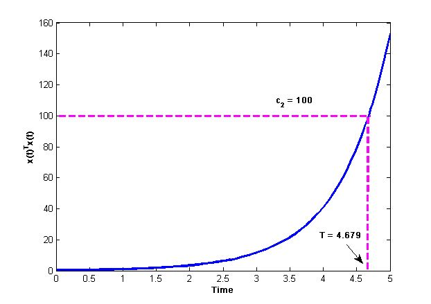
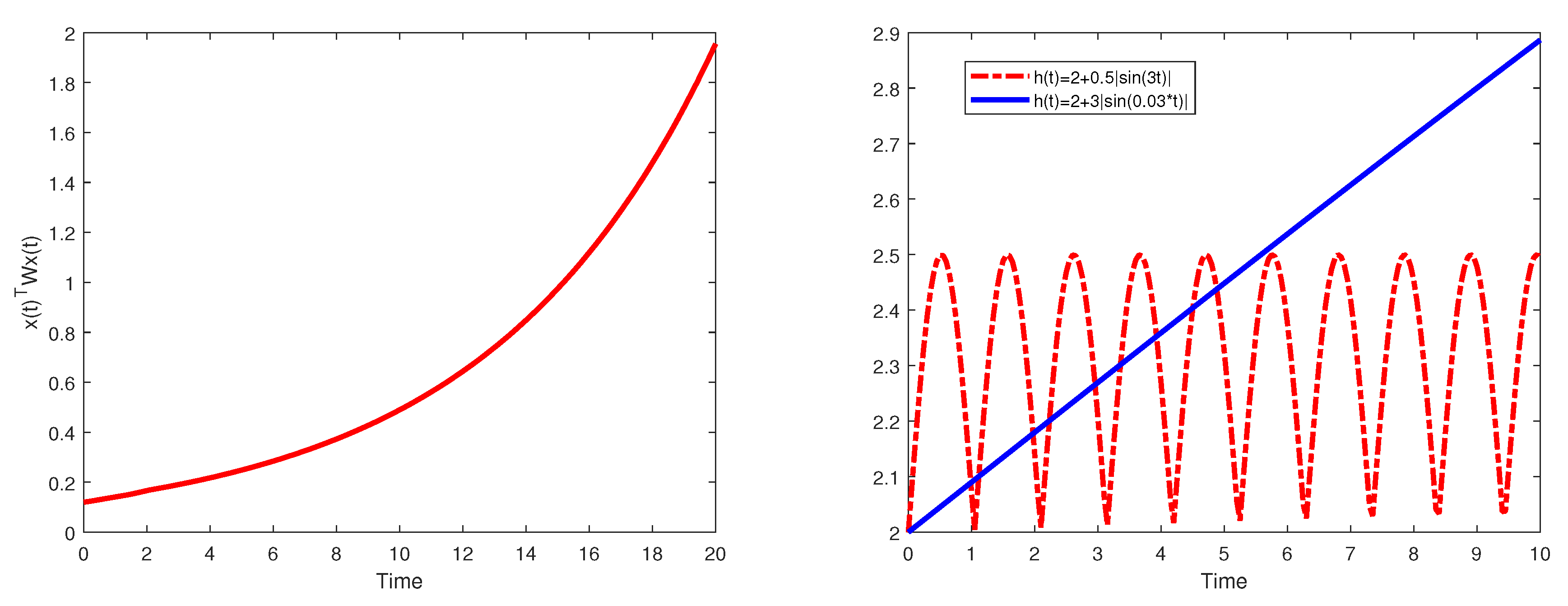
and the delay function satisfying ${\displaystyle h\left(t\right)=2+3\left|sin\right(0.03t\left)\right|}$; the uncertain parameters are given by ${\displaystyle \Delta A_0\left(t\right)=\Delta A_1\left(t\right)=0.0025sin\left(0.05t\right)I,\Delta B\left(t\right)={[0.005sin\left(0.05t\right)00]}^T}$; with an initial condition $\varphi \left(t\right)=(0.2+0.1t){\left[111\right]}^T$. The norm of solution of the uncertain linear system with $u\left(t\right)=0$ is shown in Figure 1(left). One can notice that the trajectory of $x^T\left(t\right)Wx\left(t\right)={\parallel x\left(t\right)\parallel }^2$ diverges as $t\to \infty$.

Case 1.Consider RFTS ($u\left(t\right)=0$) of this uncertain linear system with respect to parameters $c_1=0.5$, $h_1=2$, $h_2=5,W=I$ that satisfy the given initial condition and delay function above. We use MATLAB control toolbox to solve the required conditions in Theorem 1 and Corollary 1 and obtain the smallest upper bounds of $c_2$ guaranteeing RFTS with respect to $(0.5,c_2,T_f,2,5,I)$. We compare these values with ones presented in [9,10] for $T_f=10,20$. Results are listed in

Table 1. Smallest values of $c_2$ guarantee RFTS with respect to $(0.5,c_2,T_f,2,5,I)$ (Example 1: case 1).

${\mathit{T}}_{\mathit{f}}$	Theorem 1 ($\mathit{\alpha }$)	Corollary 1 ($\mathit{\alpha }$)	Therorem 7 [9]	Theorem 1 [10]
10	$502.95\left(0.317\right)$	$182.4\left(0.348\right)$	$2.7$	$1484.1$
20	$11790\left(0.314\right)$	$5745\left(0.343\right)$	$13.3$	44469

. It is clearly that values from [9] are smaller than the others for both $T_f=10,20$; while values from both of our conditions yield better results than values given in [10].

Case 2.We next investigate RFTS and RFTU of the same uncertain linear system with different delay function which is defined to be ${\displaystyle h\left(t\right)=2+0.5\left|sin\right(3t\left)\right|}$. This delay function is displayed in Figure 1(right). One can see that this delay function is non-differentiable for some $t\in [0,10]$.

Results of RFTS and RFTU with respect to $(0.5,c_2,T_f,2,2.5,I)$ of this system with ${\displaystyle h\left(t\right)=2+0.5\left|sin\right(3t\left)\right|}$ are listed in

Table 2. Smallest values of $c_2$ guarantee RFTS and RFTU with respect to $(0.5,c_2,T_f,2,2.5,I)$, $T_f=2,4,6,8,10$. (Example 1: case 2). NF means ’not FTS’.

	${\mathit{T}}_{\mathit{f}}$	2	4	6	8	10
RFTS	Theorem 1 $(\alpha =0.38)$	$12.1$	$26.49$	$56.72$	$121.29$	$259.31$
	Corollary 1 $(\alpha =0.41)$	$6.15$	$14.31$	$32.49$	$73.73$	$167.4$
	Theorem 3 [9]	NF	NF	NF	NF	NF
RFTU	Theorem 1 $(\alpha =0.37)$	$11.52$	$24.38$	$51.07$	$107.03$	$220.64$
	Corollary 1 $(\alpha =0.39)$	$5.81$	$13.01$	$28.46$	$62.09$	$135.44$

. Clearly, our Corollary 1 yields smaller values of $c_2$ for guaranteeing both RFTS and RFTU; while condition in [9] is not feasible for all cases since it requires slow changing in delay function ($\dot{h}\left(t\right)<1$).

In case of fixed $T_f=10$, solving the required conditions in Corollary 1, we obtain value of computed ${\parallel x\left(t\right)\parallel }^2\le 135.438$ and a set of feasible solutions guaranteeing RFTU of the linear system (1) with respect to $(0.5,135.44,10,2,2.5,I)$ as follow: $\alpha =0.39,{\beta }_1=0.9997,{\beta }_2=3.1873,{\beta }_3=5.4968,{\beta }_4=1.1682$, ${\beta }_5=3.5926,$

$$\begin{array}{cc}\hfill & P=\left[\begin{array}{ccc}0.999& -0.000& -0.000\\ -0.000& 0.999& 0.000\\ -0.000& 0.000& 0.999\end{array}\right],Q_1=\left[\begin{array}{ccc}4.809& -0.216& 0.026\\ -0.216& 3.748& -0.422\\ 0.026& -0.422& 3.517\end{array}\right],Q_2=\left[\begin{array}{ccc}9.482& -0.319& -0.207\\ -0.319& 6.668& -0.895\\ -0.207& -0.895& 6.233\end{array}\right],\hfill \\ \hfill & R_1=\left[\begin{array}{ccc}1.950& -0.048& -0.011\\ -0.048& 1.271& -0.076\\ -0.011& -0.076& 1.228\end{array}\right],R_3=\left[\begin{array}{ccc}4.009& -0.242& 0.140\\ -0.242& 4.350& -0.572\\ 0.140& -0.572& 4.031\end{array}\right].\hfill \end{array}$$

Here, the state-feedback control guaranteeing RFTU for $T_f=10$ is designed to be $u\left(t\right)=-0.5B^T{P}^{-1}x\left(t\right)={\left[-0.500500\right]}^{T}x\left(t\right)$.

Example 2

([17]). Consider the linear system (1) with time-varying delay but no uncertainty, no controller with matrix coefficients defined by

$$\begin{array}{cc}\hfill & A_0=\left[\begin{array}{cc}-0.2& 2\\ -1& -0.2\end{array}\right],A_1=\left[\begin{array}{cc}-0.1& -0.1\\ -0.1& 0.1\end{array}\right],D=\left[\begin{array}{cc}0& 0\\ 0& 0\end{array}\right],\hfill \end{array}$$

${\displaystyle D=E_0=E_1,B=E_2={\left[00\right]}^T,W=I=diag(1,1)}$.

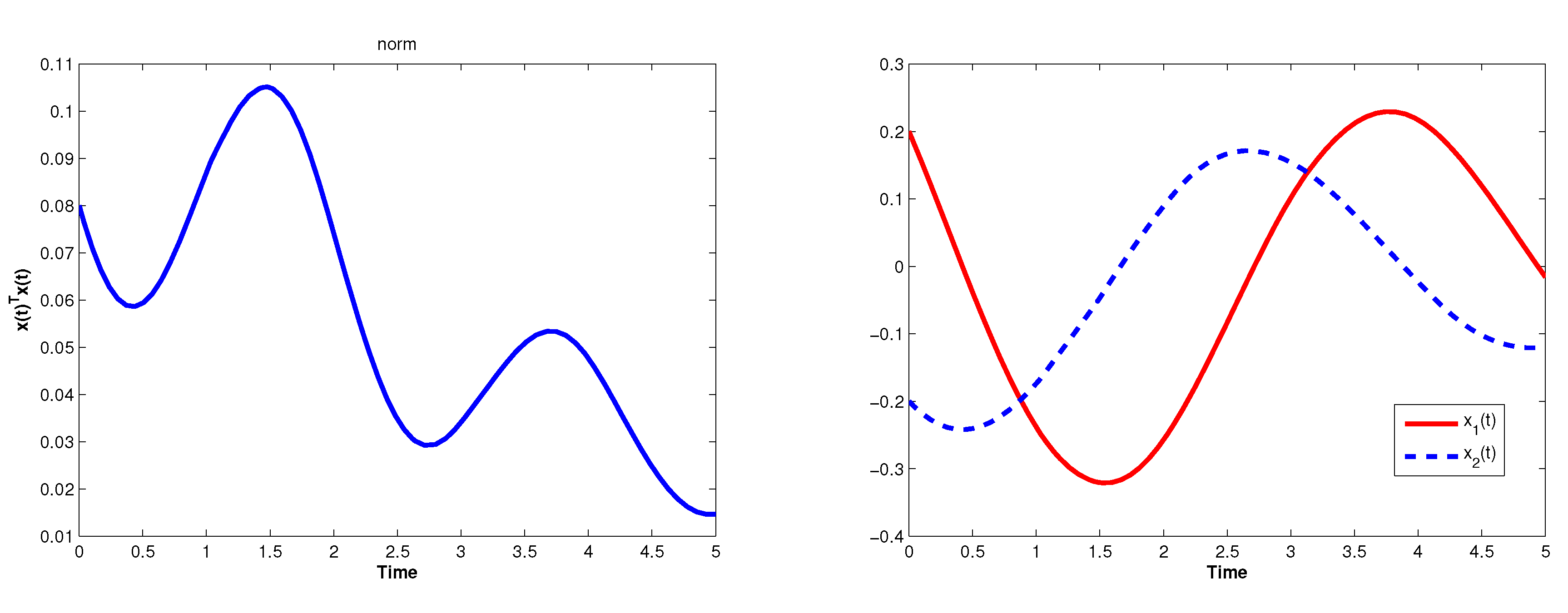
We investigate the FTS of the system with the delay function given by $h\left(t\right)=1+0.5\left|sin\right(0.03t\left)\right|$ and the initial conditions satisfying $\varphi \left(t\right)=(0.2+0.1t){[1-1]}^T$. With the given initial condition and delay function, we choose $c_1=0.18,h_1=1,h_2=1.5$. The solution of this system is shown in Figure 2. We observe that the linear system is asymptotic stable with oscillation at the early state. Thus, it is worth to investigate and compare results of FTS of the system for a short period of time; e.g., $T_f\le 5$.

By solving our proposed FTS criteria (with $u=0$), results are shown in

Table 3. Values of smallest $c_2$ guaranteeing FTS of the linear system (1) with respect to $(0.18,c_2,T_f,1,1.5,I)$ for $T_f=1,2,3,4,5$ (Example 2).

${\mathit{T}}_{\mathit{f}}$	1	2	3	4	5
Stojanovic [9]	$0.33$	$0.33$	$0.33$	$0.33$	$0.33$
Puangmalai et al. [17]	$0.41$	$0.43$	$0.45$	$0.47$	$0.49$
Zhang et al. [10]	$759.5$	${10}^6$	${10}^9$	${10}^{12}$	${10}^{15}$
Corollary 1	$5.9$	$30.7$	154	753	3727
$\left(\alpha \right)$	$\left(1.7\right)$	$\left(1.6\right)$	$\left(1.6\right)$	$\left(1.6\right)$	$\left(1.6\right)$

. For given $c_2$ and $T_f$, only conditions in Corollary 1 guarantee FTS of the considered system; while conditions in Theorem 1 does not guarantee FTS (results are not shown). By comparing with the past results, one can see that values of $c_2$ given by [9] are the best among these results; while values provided by our Corollary 1 are better than some results.

In addition, we further investigate FTS of this linear system with non-differential delay function, $h\left(t\right)=1+0.5\left|sin\right(3t\left)\right|$, on $t\in [0,5]$. Our Corollary 1 provides the same values of $c_2$ as shown in Table 3 with only results from [17] that gives better results than ours; while FTS condition from [9] does not satisfy, since it requires delay function to be differentiable.

Example 3.

Consider the linear system (1) with coefficient matrices defined by

$$\begin{array}{cc}\hfill & A_0=\left[\begin{array}{ccc}-1.7& 1.7& 0\\ 1.3& -1& 0.7\\ 0.7& 1& -0.6\end{array}\right],A_1=\left[\begin{array}{ccc}1.5& -1.7& 0.1\\ -1.3& 1& -0.5\\ -0.7& 1& 0.6\end{array}\right],\hfill \end{array}$$

(31)

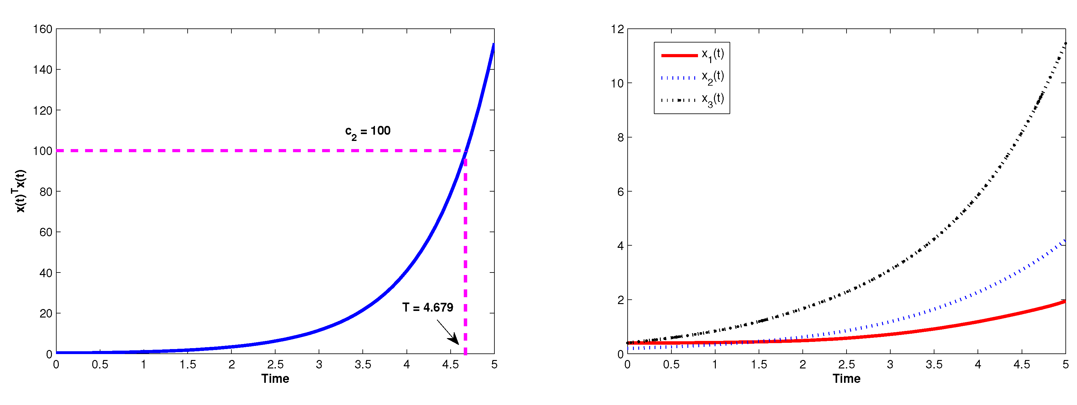
and the delay function satisfying ${\displaystyle h\left(t\right)=0.1+0.2|cos\left(t\right)|}$; the uncertain parameters are given by ${\displaystyle \Delta A_0\left(t\right)=\Delta A_1\left(t\right)=cos\left(0.03t\right)diag(0.000025,0.000001,0.0001),\Delta B\left(t\right)={[0.001cos\left(0.03t\right)00]}^T}$. With an initial condition $\varphi \left(t\right)={\left[0.40.20.4\right]}^T$, the solution of the system are shown in Figure 3. One can notice that the trajectory of $x^T\left(t\right)Wx\left(t\right)={\parallel x\left(t\right)\parallel }^2$ diverges as $t\to \infty$. To further investigate the (R)FTS and (R)FTU, we can choose values of $c_1=0.36,h_1=0.1,h_2=0.3$ that satisfy the given initial condition and delay function above.

Case 1.Consider the linear system (1) with coefficient matrices defined in (31) and uncertainties satisfying ${\displaystyle D=E_0=E_1=diag(0.005,0.001,-0.01)}$ but no controller; i.e., $B={\left[000\right]}^T$.

Now, we investigate the RFTS of this system with respect to $(c_1,c_2,T_f,h_1,h_2,W)=(0.36,c_2,T_f,0.1,0.3,I)$ for various values of given $c_2$ and $T_f$. By solving the inequalities and LMIs in Theorem 1 and Corollary 1, values of the smallest upper bounds (up to 3 decimal digits) of computed $x^T\left(t\right)Wx\left(t\right)={\parallel x\left(t\right)\parallel }^2$ are listed in

Table 4. Smallest upper bounds of computed $x^T\left(t\right)Wx\left(t\right)={\parallel x\left(t\right)\parallel }^2,t\in [0,T_f]$ for given $c_2$ guaranteeing RFTS with respect to $(0.36,c_2,T_f,0.1,0.3,I)$ of linear system with uncertainties (example 3: case 1). NF means ’not FTS’.

		Computed ${\parallel \mathit{x}\left(\mathit{t}\right)\parallel }^2$ and Value of ($\mathit{\alpha }$)
${\mathbf{T}}_{\mathit{f}}$	Fixed ${\mathit{c}}_{\mathbf{2}}$	Theorem 1	Corollary 1	Fixed ${\mathit{c}}_{\mathbf{2}}$	Theorem 1	Corollary 1
1	$11.6$	$11.598\left(2.1\right)$	$10.354\left(2.3\right)$	7	NF	$6.992\left(2.4\right)$
2	75	$74.968\left(1.7\right)$	$70.362\left(1.8\right)$	54	NF	$53.856\left(1.9\right)$
3	400	$399.276\left(1.6\right)$	$385.776\left(1.7\right)$	320	NF	$319.727\left(1.7\right)$
4	2000	$1995.7\left(1.6\right)$	$1961.7\left(1.7\right)$	1750	NF	$1748.7\left(1.7\right)$
5	9500	$9490\left(1.5\right)$	$9499\left(1.7\right)$	9330	$9329\left(1.5\right)$	NF

. For instance, fixed $T_f=1$, conditions in Theorem 1 and Corollary 1 guarantee RFTS with given smallest values of $c_2$ (with smallest upper bounds of computed ${\parallel x\left(t\right)\parallel }^2$) of $11.6$ ($11.598$) and 7 ($6.992$), respectively. From Table 4, one can see that values of $c_2$ guaranteeing RFTS obtained from Corollary 1 are smaller than those provided by Theorem 1 in most cases, except the case of $T_f=5$ that Theorem 1 allows smaller value of $c_2$. Note that this is also true for $T_f\ge 5$. However, these smallest upper bounds of $c_2$ are still large comparing to the actual values of ${\parallel x\left(t\right)\parallel }^2$ for fixed $t=T_f$ as seen in Figure 3(left).

We continue investigate the maximum values of $T_f$ that guarantee RFTS of the linear system (1) with respect to $(0.36,c_2,T_f,0.1,0.3,I)$, for fixed $c_2$. Results are shown in

Table 5. Maximum $T_f$ guarantees RFTS of the delay linear system (1) with respect to $(0.36,c_2,T_f,0.1,0.3,I)$ for fixed $c_2$ (Example 3: case 1).

${\mathit{c}}_2$	10	50	100	500	1000	5000	10,000	50,000
Theorem 1	$0.933$	$1.768$	$2.172$	$3.154$	$3.588$	$4.593$	$5.046$	$6.1198$
$\left(\alpha \right)$	$\left(2.2\right)$	$\left(1.8\right)$	$\left(1.7\right)$	$\left(1.6\right)$	$\left(1.6\right)$	$\left(1.6\right)$	$\left(1.5\right)$	$\left(1.5\right)$
Corollary 1	$1.165$	$1.972$	$2.353$	$3.268$	$3.676$	$4.623$	$5.030$	$5.977$
$\left(\alpha \right)$	$\left(2.2\right)$	$\left(1.9\right)$	$\left(1.8\right)$	$\left(1.7\right)$	$\left(1.7\right)$	$\left(1.7\right)$	$\left(1.7\right)$	$\left(1.7\right)$

. For fixed $c_2=100$, both of our proposed conditions guarantee ${\parallel x\left(t\right)\parallel }^2\le 100$ for $t\in [0,2.353]$ (from Corollary 1). Note that the true values of ${\parallel x\left(t\right)\parallel }^2\le 100$ for all $t\le 4.679$ (see Figure 3(left)). It is clearly that the larger values of $c_2$ allows larger values of $T_f$ guaranteeing RFTS. One can observe that, for $c_2\le 5000$, Corollary 1 allows larger values of $T_f$ than those provided by Theorem 1.

Case 2.Consider the RFTU of the linear system (1) with coefficient matrices giving in (31) and uncertainties satisfying ${\displaystyle D=diag(0.005,0.001,-0.01),E_0=E_1=D,E_2={\left[0.200\right]}^T}$, and $B={\left[-112\right]}^T$.

The smallest upper bounds of computed ${\parallel x\left(t\right)\parallel }^2$ provided by Theorem 1 and Corollary 1 are listed in

Table 6. Smallest upper bounds of computed $x^T\left(t\right)Wx\left(t\right)={\parallel x\left(t\right)\parallel }^2,t\in [0,T_f]$ for given $c_2$ guaranteeing FTS with respect to $(0.36,c_2,T_f,0.1,0.3,I)$ of linear system with uncertainties and controller (Example 3: case 2). NF means ’not FTS’.

		Computed ${\parallel \mathit{x}\left(\mathit{t}\right)\parallel }^2$ and Value of ($\mathit{\alpha }$)
${\mathbf{T}}_{\mathit{f}}$	Fixed ${\mathit{c}}_{\mathbf{2}}$	Theorem 1	Corollary 1	Fixed ${\mathit{c}}_{\mathbf{2}}$	Theorem 1	Corollary 1
1	$3.5$	$3.499\left(1.7\right)$	$2.199\left(0.5\right)$	$1.25$	NF	$1.249\left(0.8\right)$
2	16	$15.997\left(1.4\right)$	$3.956\left(0.2\right)$	$2.09$	NF	$2.090\left(0.2\right)$
3	64	$63.974\left(1.3\right)$	$4.600\left(0.2\right)$	$2.35$	NF	$2.349\left(0.1\right)$
4	245	$244.248\left(1.3\right)$	$5.348\left(0.1\right)$	$2.59$	NF	$2.589\left(0.1\right)$
5	900	$897.203\left(1.3\right)$	$5.769\left(0.1\right)$	$2.86$	NF	$2.859\left(0.1\right)$

. We observe that the computed upper bounds of ${\parallel x\left(t\right)\parallel }^2$ are smaller, when controllers are given, comparing to those obtained in Case 1 (no controllers). In other words, with designed controller, the linear system (1) can maintain its normed trajectory to be within certain values of $c_2$ with longer time $T_f$.

In case of fixed $T_f=5$, solving the required conditions in Corollary 1, we obtain value of computed ${\parallel x\left(t\right)\parallel }^2\le 2.859$ and a set of feasible solutions guaranteeing RFTU of the linear system (1) with respect to $(0.36,2.86,5,0.1,0.3,I)$ as follow: $\alpha =0.1,{\beta }_1=0.266,{\beta }_2=0.328,{\beta }_3=0.502,{\beta }_4=0.275,{\beta }_5=0.317,$

$$\begin{array}{cc}\hfill & P=\left[\begin{array}{ccc}0.928& -0.189& -0.093\\ -0.189& 0.424& -0.221\\ -0.093& -0.221& 0.869\end{array}\right],Q_1=\left[\begin{array}{ccc}0.994& -0.207& -0.276\\ -0.207& 0.437& -0.099\\ -0.276& -0.099& 1.253\end{array}\right],Q_2=\left[\begin{array}{ccc}1.104& -0.235& -0.471\\ -0.235& 0.604& 0.078\\ -0.471& 0.078& 1.981\end{array}\right],\hfill \\ \hfill & R_1=\left[\begin{array}{ccc}0.945& -0.185& -0.171\\ -0.185& 0.414& -0.168\\ -0.171& -0.168& 1.004\end{array}\right],R_3=\left[\begin{array}{ccc}0.956& -0.141& -0.239\\ -0.141& 0.395& -0.133\\ -0.239& -0.133& 1.186\end{array}\right].\hfill \end{array}$$

Here, the state-feedback control guaranteeing robust FTS for $T_f=5$ is designed to be $u\left(t\right)=-0.5B^T{P}^{-1}x\left(t\right)=\left[-0.0543-2.00823-1.6861\right]x\left(t\right)$.

Case 3.Consider the FTS of the delay linear system (1) with coefficient matrices given in (31) but all uncertainty matrices are zero matrices and no controller.

In this case, we solve the required conditions in Theorem 1 and Corollary 1 and obtain smallest values of $c_2$ guaranteeing FTS for fixed $T_f$ as listed in

Table 7. Smallest values of $c_2$ guaranteeing FTS of linear system with respect to $(0.36,c_2,T_f,0.1,0.3,I)$ (Example 3: case 3) for fixed $T_f$.

${\mathit{T}}_{\mathit{f}}$	1	2	3	4	5
Theorem 1	$11.56$	$74.8$	391	1935	9313
$\left(\alpha \right)$	$\left(2.1\right)$	$\left(1.7\right)$	$\left(1.6\right)$	$\left(1.6\right)$	$\left(1.5\right)$
Corollary 1	$6.92$	$52.7$	317	1735	9490
$\left(\alpha \right)$	$\left(2.3\right)$	$\left(1.9\right)$	$\left(1.7\right)$	$\left(1.7\right)$	$\left(1.7\right)$

. One can notice that condition from Corollary 1 allows smaller values of $c_2$ guaranteeing FTS than those obtained from Theorem 1 for each $T_f=1,2,3,4$; while condition from Theorem 1 allows the smaller value of $c_2$ guaranteeing FTS for $T_f\ge 5$ (results for $T_f>5$ are omitted). In addition, we also investigate the maximum of $T_f$ allowing FTS of the linear system (1) with respect to $(0.36,c_2,T_f,0.1,0.3,I)$. The maximum values of $T_f$ guaranteeing FTS from both criteria (results of this case are not shown here) are very close to those shown in Table 5 with slightly larger values of $T_f$ in this case for each given $c_2$. This result implies that the uncertainties may be the cause of shortening the maximum $T_f$ guaranteeing RFTS in case 1.

Case 4.Consider the FTU of the delay linear system (1) with coefficient matrices given in (31) with a designed controller but no uncertainties; i.e., setting $D=0$.

The smallest upper bounds of computed ${\parallel x\left(t\right)\parallel }^2$ obtained from the proposed criteria are listed in

Table 8. Smallest upper bounds of computed ${\parallel x\left(t\right)\parallel }^2,t\in [0,T_f]$ for given $c_2$ guaranteeing FTU with respect to $(0.36,c_2,T_f,0.1,0.3,I)$ of linear system with controller but no uncertainty (Example 3: case 4).

		Computed ${\parallel \mathit{x}\left(\mathit{t}\right)\parallel }^2$ and Value of ($\mathit{\alpha }$)
${\mathbf{T}}_{\mathit{f}}$	Fixed ${\mathit{c}}_{\mathbf{2}}$	Theorem 1	Corollary 1	Fixed ${\mathit{c}}_{\mathbf{2}}$	Theorem 1	Corollary 1
1	$3.39$	$3.389\left(1.6\right)$	$2.221\left(0.7\right)$	$1.24$	NF	$1.239\left(0.9\right)$
2	$14.9$	$14.899\left(1.4\right)$	$3.638\left(0.2\right)$	$2.08$	NF	$2.079\left(0.2\right)$
3	$56.4$	$56.394\left(1.3\right)$	$4.432\left(0.1\right)$	$2.33$	NF	$2.329\left(0.1\right)$
4	207	$206.975\left(1.3\right)$	$5.293\left(0.1\right)$	$2.58$	NF	$2.579\left(0.1\right)$
5	759	$758.920\left(1.3\right)$	$5.815\left(0.1\right)$	$2.85$	NF	$2.848\left(0.1\right)$

. Smaller values of $c_2$ are allowed by Corollary 1 than those are provided by in Theorem 1 to guarantee FTU of the delay linear system (1) for each fixed $T_f=1,2,3,4,5$. For $T_f=5$, we design a state-feedback controller in the form: $u\left(t\right)=-0.5B^T{P}^{-1}x\left(t\right)=\left[-0.0520-2.0639-1.6788\right]x\left(t\right)$ in Corollary 1. A set of feasible solutions guaranteeing FTU of the system with respect to $(0.36,2.86,5,0.1,0.3,I)$ is: $\alpha =0.1,{\beta }_1=0.267,{\beta }_2=0.329,{\beta }_3=0.501,{\beta }_4=0.282,{\beta }_5=0.318,$

$$\begin{array}{cc}\hfill & P=\left[\begin{array}{ccc}0.928& -0.190& -0.093\\ -0.190& 0.426& -0.220\\ -0.093& -0.220& 0.869\end{array}\right],Q_1=\left[\begin{array}{ccc}0.994& -0.207& -0.276\\ -0.207& 0.437& -0.099\\ -0.276& -0.099& 1.253\end{array}\right],Q_2=\left[\begin{array}{ccc}1.098& -0.230& -0.466\\ -0.230& 0.600& 0.077\\ -0.466& 0.077& 1.982\end{array}\right],\hfill \\ \hfill & R_1=\left[\begin{array}{ccc}0.942& -0.183& -0.167\\ -0.183& 0.414& -0.169\\ -0.167& -0.169& 0.999\end{array}\right],R_3=\left[\begin{array}{ccc}0.952& -0.139& -0.234\\ -0.139& 0.394& -0.134\\ -0.234& -0.134& 1.174\end{array}\right].\hfill \end{array}$$

Remark 5.

With the given uncertain parameters ${\displaystyle \Delta A_0\left(t\right)=\Delta A_1\left(t\right)=0.0025sin\left(0.05t\right)I,\Delta B\left(t\right)={[0.005sin\left(0.05t\right)00]}^T}$, in Example 1. These parameters are equivalent to assume ${\displaystyle D=E_0=E_1=diag(0.05,0.05,0.05),E_2={\left[0.100\right]}^T}$ and ${\displaystyle \Delta \left(t\right)=sin\left(0.05t\right)I}$ where $I=diag(1,1,1)$. In Example 3, the given uncertain parameters ${\displaystyle \Delta A_0\left(t\right)=\Delta A_1\left(t\right)=cos\left(0.03t\right)diag(0.000025,0.000001,0.0001),\Delta B\left(t\right)={[0.001cos\left(0.03t\right)00]}^T}$ are equivalent to choose ${\displaystyle D=E_0=E_1=diag(0.005,0.001,-0.01),E_2={\left[0.200\right]}^T}$ and ${\displaystyle \Delta \left(t\right)=cos\left(0.03t\right)I}$.

Remark 6.

From simulations in Examples 1 and 2, our proposed sufficient can guarantee (R)FTS and (R)FTU with non-differentiable delay function. Note that the conditions given in [9] yield the best results among the existing researches for differentiable delay function but these conditions cannot be applied to guarantee (R)FTS in case of non-differentiable or rapid delay functions, since they require $\dot{h}\left(t\right)<1$.

Remark 7.

From Example 3, we observe that the Corollary 1 guarantees (R)FTS or (R)FTU with smaller values of $c_2$ for each $T_f=1,2,3,4$, except $T_f\ge 5$. For $T_f\ge 5$, Theorem 1 allows smaller value of $c_2$ to guarantee (R)FTS of the linear system without controller (cases 1 and 3); however, when controller is designed, Corollary 1 allows lower values of $c_2$ for each $T_f$.

Remark 8.

Sufficient stability condition of the dynamical system that guarantees (R)FTS or (R)FTU with smaller value of $c_2$ would help us know the limits or bounds of norm of state variables. In practical system, these smallest values of $c_2$ give information for designing a safety system; while the maximum $T_f$ tells us how long the norm of state variable can stay within the certain limits. We also notice, from cases 1 and 3 in Example 3, that the uncertainties may be the cause for shortening the maximum time $T_f$ guaranteeing FTS.

5. Discussion and Conclusions

In this article, the robust finite-time stability and stabilization criteria of linear system (1) with time-varying delay and uncertainties have been formulated based on LKFs. These sufficient conditions are given in the forms of inequalities and LMIs. We apply the Cauchy-like matrix inequality to handle the nonlinear terms appearing in the derivation procedure; unlike some of the past researches that define them as new variables. In addition, our proposed conditions can be applied to linear system with non-differentiable time-varying delay. Thus, our sufficient RFTS and RFTU conditions are less conservative than some of the past researches. Three numerical examples have been presented to show the effect of using slightly different forms of LKFs in the main results. Numerical results show that having less terms in LKFs (as in Corollary 1) may allow better result (lower $c_2$) for guaranteeing (R)FTS or (R)FTU of the linear system (1). The impacts of using more (complicated) terms in LKFs are required further investigation. We also investigate the RFTU condition by applying the same derivation procedure of our main theorems but using the Wirtinger inequality for bounding the integral terms appearing in the derivative of LKFs. We observe that the sufficient RFTU conditions using the Wirtinger inequality do not guarantee RFTU in our numerical simulations. Note that RFTU criteria using the Wirtinger inequality are not presented here.

References

- Wang, H.; Yuan, Z.; Chen, B.; He, X.; Zhao, J.; Qiu, T. Analysis of the stability and controllability of chemical processes. Comput. Chem. Eng. 2011, 35, 1101–1109. [Google Scholar] [CrossRef]
- Kot, M. Elements of Mathematical Ecology; Cambridge University Press: Cambridge, UK, 2001. [Google Scholar]
- Cole, J.D.; Greifinger, C. Acoustic gravity waves from an energy source at the ground in an isothermal atmosphere. J. Geophys. Res. 1969, 74, 3693–3703. [Google Scholar] [CrossRef]
- Hariharan, S.I. A model problem for acoustic wave propagation in the atmosphere. In Proceedings of the First IMACS Symposium on Computer Acoustics; Lee, D., Sternberg, R.L., Schultz, M.H., Eds.; NorthHolland Publishing Company: Amsterdam, The Netherlands, 1988; pp. 65–82. [Google Scholar]
- Vimal Kumar, S.; Raja, R.; Marshal Anthoni, S.; Cao, J.; Tu, Z. Robust finite-time non-fragile sampled-data control for T-S fuzzy flexible spacecraft model with stochastic actuator faults. Appl. Math. Comput. 2018, 321, 483–497. [Google Scholar] [CrossRef]
- Rajakumar, V.; Anbukumar, K.; Arunodayaraj, I.S. Power quality enhancement using linear quadratic regulator based current-controlled voltage source inverter for the grid integrated renewable energy system. Electr. Power Compon. Syst. 2017, 45, 1783–1794. [Google Scholar] [CrossRef]
- Amato, F.; Ariola, M.; Cosentino, C. Robust finite-time stabilisation of uncertain linear systems. Int. J. Control 2011, 84, 2117–2127. [Google Scholar] [CrossRef]
- Niamsup, P.; Phat, V.N. Robust finite-time control for linear time-varying delay systems with bounded control. Asian J. Control 2016, 18, 2317–2324. [Google Scholar] [CrossRef]
- Stojanovic, S.B. Further improvement in delay-dependent finite-time stability criteria for uncertain continuous-time systems with time varying delays. IET Control Theory Appl. 2016, 10, 926–938. [Google Scholar] [CrossRef]
- Zhang, Z.; Zhang, Z.; Zhang, H. Finite-time stability analysis and stabilization for uncertain continuous-time system with time-varying delay. J. Franklin Inst. 2015, 352, 1296–1317. [Google Scholar] [CrossRef]
- Seuret, A.; Gouaisbaut, F. Wirtinger-based integral inequality: Application to time-delay systems. Automatica 2013, 49, 2860–2866. [Google Scholar] [CrossRef] [Green Version]
- Botmart, T.; Niamsup, P.; Phat, V.N. Delay-dependent exponential stabilization for uncertain linear systems with interval non-differentiable time-varying delays. Appl. Math. Comput. 2011, 217, 8236–8247. [Google Scholar] [CrossRef]
- Keadnarmol, P.; Rojsiraphisal, T. Globally exponential stability of a certain neutral differential equation with time-varying delays. Adv. Differ. Equ. 2014, 32. [Google Scholar] [CrossRef] [Green Version]
- Garica-Gonzalez, P.; Garcia-Cerrada, A. Control system for a PWM-based STATCOM. IEEE Trans. Power Deliv. 2000, 15, 1252–1257. [Google Scholar] [CrossRef]
- Debeljkovic, D.L.; Stojanovic, S.B.; Jovanovic, A.M. Finite-time stability of continuous time delay systems: Lyapunov-like approach with Jensen’s and Coppel’s inequality. Acta Polytech. Hung. 2013, 10, 135–150. [Google Scholar]
- Lazarevic, M.P.; Debeljkovic, D.L.; Nenadic, Z.L.; Milinkovic, S.A. Finite-time stability of delayed systems. IMA J. Math. Control Inf. 2000, 17, 101–109. [Google Scholar] [CrossRef]
- Puangmalai, J.; Tongkum, J.; Rojsiraphisal, T. Finite-time stability criteria of linear system with non-differentiable time-varying delay via new integral inequality. Math. Comput. Simul. 2020, 171, 170–186. [Google Scholar] [CrossRef]
- Amato, F.; Ariola, M.; Cosentino, C. Finite-time stabilization via dynamic output feedback. Automatica 2006, 42, 337–342. [Google Scholar] [CrossRef]
- Lin, X.; Liang, K.; Li, H.; Jiao, Y.; Nie, J. Finite-time stability and stabilization for continuous systems with additive time-varying delays. Circ. Syst. Signal Process. 2017, 36, 2971–2990. [Google Scholar] [CrossRef]
- Liu, H.; Shi, P.; Karimi, H.R.; Chadli, M. Finite-time stability and stabilisation for a class of nonlinear systems with time-varying delay. Int. J. Syst. Sci. 2016, 47, 1433–1444. [Google Scholar] [CrossRef]
- Rojsiraphisal, T.; Puangmalai, J. An improved finite-time stability and stabilization of linear system with constant delay. Math. Probl. Eng. 2014, 154769. [Google Scholar] [CrossRef]
- Stojanovic, S.B.; Debeljkovic, D.L.; Antic, D.S. Finite-time stability and stabilization of linear time-delay systems. Facta Univ. Automat. Control Robot. 2012, 11, 25–36. [Google Scholar]
- Zamart, C.; Rojsiraphisal, T. Finite-time stabilization of Linear Systems with time-varying delays using new integral inequalities. Thai J. Math. 2019, 17, 173–191. [Google Scholar]
- Ruan, Y.; Huang, T. Finite-Time Control for Nonlinear Systems with Time-Varying Delay and Exogenous Disturbance. Symmetry 2020, 12, 447. [Google Scholar] [CrossRef] [Green Version]
- Bos, A. Parameter Estimation for Scientists and Engineers; Wiley: Hoboken, NJ, USA, 2007. [Google Scholar]
Figure 1.
Time history of (left) and 2 delay functions (right) used in Example 1.
Figure 2.
Time history of (left) and state variables (right) with for (Example 2).
Figure 3.
Time history of (left) and state variables (right) with IC of Example 3.