Nonlocal Mechanical Behavior of Layered Nanobeams


1
Department of Structures for Engineering and Architecture, University of Naples Federico II, Via Claudio 21, 80121 Naples, Italy
2
Faculty of Engineering, Department of Engineering Mechanics, University of Rijeka, Vukovarska 58, 51000 Rijeka, Croatia
*
Author to whom correspondence should be addressed.
Symmetry 2020, 12(5), 717; https://doi.org/10.3390/sym12050717
Submission received: 28 February 2020
/
Revised: 23 April 2020
/
Accepted: 28 April 2020
/
Published: 2 May 2020
(This article belongs to the Special Issue Time and Space Nonlocal Operators in Structural Mechanics)
Abstract
:The research at hand deals with the mechanical behavior of beam-like nanostructures. Nanobeams are assembled of multiple layers of different materials and geometry giving a layered nanobeam. To properly address experimentally noticed size effects in structures of this type, an adequate nonlocal elasticity formulation must be applied. The present model relies on the stress-driven integral methodology that effectively circumvents known deficiencies of other approaches. As a main contribution, a set of differential equations and boundary conditions governing the underlaying mechanics is proposed and applied to two benchmark examples. The obtained results show the expected stiffening nonlocal behavior exhibiting most of smaller and smaller structures and modern devices.
1. Introduction
The mechanical behavior at the micro- and nanoscale is governed by different forces and potentials than the macroscale structures [1]. It is well-established that relations between forces and displacements are influenced by small dimensions of such structures, nowadays widely employed to model nanocomposites [2,3] and new-generation devices, such as micro-bridges [4], nano-switches [5], nano-generators [6], and energy harvesters [7,8,9]. In other words, the whole neighborhood of a point contributes to these relations and the term nonlocal is appropriately used in these circumstances. For instance, early experimental observations [10] find that silicon is strongly influenced by size-effects. Measurements show that Young’s modulus varies from approximately 80 GPa for lower nanocantilever thicknesses, converging to 170 GPa for higher thicknesses. The upper limit value corresponds to bulk silicon. For the investigation at hand, beams assembled of several layers of different materials are of particular interest. Thin metal films are typically used in such applications. Bending load is often introduced by means of contactless electrostatic attraction. In [11], an experimental analysis of a nanocantilever made of copper and silicon layers is presented. It is found that the rather high Young’s modulus of copper (approximately 750 GPa) for low thicknesses decreases dramatically with the increase in thickness, converging to about 120 GPa. Hence, to analyze structures of such small dimensions, one needs a different mechanical apparatus than the macroscale engineer.
The aforesaid experimental observations triggered the high interest of researchers of different specialties. A detailed insight into the size-effects of nanostructures can be achieved by the molecular dynamics (MD) [12] or molecular structural mechanics [13,14,15]. Such simulations can be computationally intensive and, at least for applications involving sensors, analytical nonlocal beam models are preferred. To complicate the issue even further, most of the results dealing with the laminated beams fall within the scope of dynamics and cover a variety of boundary conditions, geometry, and loadings. As an illustration, several examples are mentioned. In [16], a nonlinear finite element analysis of the bending of a rotating laminated nanocantilever is analyzed. The vibrational framework for electro-magneto-elastic bending analysis of three-layer nanobeams is presented in [17]. The differential formulation involving the stress gradient is used. The formulation is extended to curved nanobeams in [18]. Attempts to include temperature effects can also be found (see [19,20]). Feng et al. [20] clearly demonstrated that both the cantilever dimensions and even small temperature changes contribute to the statics and dynamics of layered nanocantilevers.
The influence of the interface and surface effects in layered nanobeams is analyzed in [21] by means of analytical models. Although the approach relies on a different size effect methodology than this paper, some results have to be pointed out. In particular, the interface and surface effects can have in some configurations (especially in beams with a large length/thickness ratio) a profound influence on the elastic deformation; thus, a nonlinear analysis incorporating these effects could be more suitable. An interested reader is referred to the work of Müller and Saúl [22] for a comprehensive analysis on the subject and that of Miller and Shenoy [23] for another approach to size-dependent behavior of nanosized structural elements, nanoplates and nanobeams in particular. When dynamics of coated layered beams of microscopic thickness is to be addressed, then a surface model including damping can also have an important role. For instance, Rongong et al. [24] presented an experimental work about a novel damping layered coating, reporting important properties of the damping layer. Other sources [25,26] report that experimental verification in some cases confirms the importance of the interface effects, while in other cases the interface effects can be disregarded. Thus, one should carefully study the layered beam in question to decide if the surface and interface effects are important or not.
Most of the previous efforts are related to the gradient-based nonlocal formulation. The original theory, as proposed by Eringen [27], is based on the strain-driven integral convolution leading to an equivalent gradient formulation. These results became a popular starting point for many nonlocal applications in mechanics. However, the theory involves some assumptions that are frequently overlooked. In particular, the original contribution was developed to describe surface waves in unbounded continua, thus applications to bounded continua such as beams or plates can be affected by a non-physical behavior. To assure equivalence of the integral and gradient formulation, a suitable set of boundary conditions must be provided. Unfortunately, these boundary conditions contradict equilibrium constraints, as shown in [28,29]. The paradoxical behavior has been known to occur [30,31] for quite some time. This is particularly true for the nanocantilever with a tip loading, a frequently used nanostructure. An efficient answer to this problem is the stress-driven integral formulation [29,32] in which the strain state at a point is influenced by the stress distribution in the neighborhood. It also introduces the constitutive boundary conditions necessary for the correct solution of the equivalent differential formulation. In strong contrast to existing formulations, the present research takes the stress-drive integral formulation as the starting point.
This paper aims to contribute to the current body of literature on the mechanics of small-scale structures in nonlocal integral elasticity. To this end, the stress-driven integral formulation [32] is extended in the present paper to effectively capture scale phenomena in composite beams made of an arbitrary number of layers of different constitutive materials, with an arbitrary width of each layer. The presented model can accommodate beams simultaneously loaded by axial and bending loads.
2. Fundamental Concepts
2.1. Geometry of the Beam
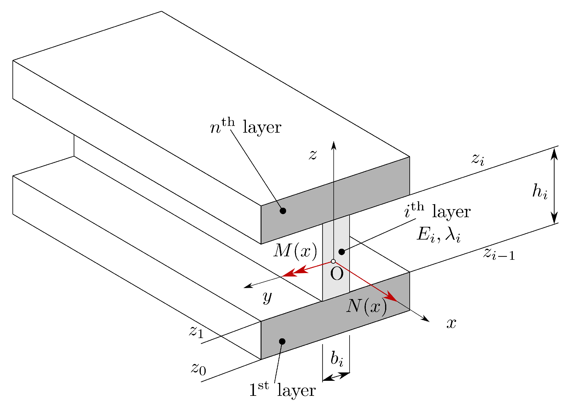
The present section defines assumptions regarding the geometry for beams assembled of n layers of different materials (Figure 1). Bending in the plane is analyzed by means of the Bernoulli–Euler formulation. We select the x-axis as the longitudinal axis, while the vertical position of the origin of the coordinate system is situated at the geometric centroid of the cross-section. Therefore, some layer is represented by the rectangular cross-section of height . It is assumed that coordinates and define the upper and lower side of layer i. The width is defined in the y direction, i.e., orthogonal to the bending plane. Indices throughout the paper denote the layer number and are not used in the sense of the Einstein summation convention. The beam’s length is denoted by L.
Thus, the cross-section of the beam is assumed to be composed of n rectangles. If the cross-section is symmetric with respect to the plane and if the origin of the coordinate system O is situated at the centroid, then the first moment of area must vanish:
However, due to differences in the Young’s modulus of each layer, the physical neutral surface in which the normal stresses vanish does not correspond in general to the geometrical middle surface [33]. A similar situation occurs in functionally graded beams along the vertical coordinate z (see [34,35,36]). The distance between these two surfaces is denoted by .
2.2. Notation
To simplify elaborations, new notation for vectors describing geometry and material of layers can be introduced in a more compact manner as:
where the last vector consists of n ones and the symbol ⊙ represents the Hadamard product, i.e., the component-wise multiplication of two vectors. Elements of the vector are widths and heights of each layer; and , , and contain cross-section areas and first and second moments of cross-section area for each layer, respectively. Young’s moduli of layers are given as elements of . The nonlocal parameters that are described below are given in . Although using boldface uppercase Latin letters violates standard vector notation, its meaning is hopefully more easily interpreted by readers due to familiarity to the equivalent scalar notation.
The following scalar quantities describing local stiffnesses are also introduced
while the nonlocal contributions are denoted by
The symbol · denotes the scalar product of two vectors as usual.
2.3. Kinematics of the Beam
The presence of the shift of neutral surface requires the modification of the standard equation representing the longitudinal displacement of each point in the plane:
The first term is an average longitudinal displacement due to axial loading. Differences in the stiffness of each layer are causing the variation of the longitudinal displacement in the transverse direction even in the simplest case of axial loading. In that way, it is more convenient to work with an average longitudinal displacement. The average longitudinal displacement in a particular cross-section x can be evaluated as:
where is the total cross-section area. The second term in Equation (5) accounts for the rotation of the cross-section due to bending loads.
The Bernoulli–Euler hypothesis imposes the absence of the shear stresses and thus relates the transversal displacement in the direction of the z-axis and angle of rotation in a usual manner:
where the apex denotes the nth derivative with respect to x. Differentiation of the longitudinal displacement with respect to x now gives the normal strain:
3. Nonlocal Material Model
Application of the stress-driven nonlocality within the beam framework was initially introduced in a series of papers [29,32] to overcome applicative difficulties of the strain-driven purely nonlocal approach [28]. The same concept can be adopted for layered beams as well. The normal strain in some layer i depends on the axial stress in the neighborhood, and the closest points have more influence than the more distant ones:
The kernel function can be selected in several ways. In this particular instance, the exponential form is conveniently chosen. The kernel is a function of a single variable—the longitudinal coordinate x—thus only normal stresses in points with the same coordinate z contribute to the nonlocality:
The parameter governing nonlocal behavior is the characteristic length , where is the small-size parameter of a particular material layer. The reader should be warned that the value of this parameter for a particular material is still unknown in most cases. The parameter should be ideally determined experimentally, but this is rarely done so (see [37,38,39] for some attempts). Alternatively, molecular dynamics or molecular structural mechanics can be employed [15,40,41,42,43,44] for the purpose, but the reported results also indicate that the precise value of the small-size parameter is far from being accurately determined.
The equivalent differential problem can be stated in each layer as [45,46]:
with the following boundary conditions:
In the context of beams, the nonlocal framework involving stresses and strains is not that useful. The usual practice is to work with displacements and stress resultants. The normal force in the cross-section follows from the balance of the linear momentum:
Likewise, the bending moment follows from the balance of the angular momentum:
Above, the vectors and represent the contribution of each layer to total stress resultants.
The problem in Equations (11) and (12) can now be expressed in the setting involving the displacements and stress resultants. In the first step, the kinematics of the beam in Equation (8) is exploited to obtain:
and constraints
The latter non-standard constraints are constitutive boundary conditions. Introducing the stress in Equation (15) into the stress resultant , Equation (13) yields the contribution of each layer to the total :
For the complete cross-section, this can be represented by means of the vectorial representation:
Scalar multiplication by gives:
or more compactly:
A similar procedure can be applied to the constitutive boundary conditions in Equation (16) which become:
As for the bending moment, the same steps are followed. Starting from the normal stresses in Equation (15) that are multiplied by , it is obtained:
The constitutive boundary conditions are:
This completes the nonlocal stress-driven beam relations between the displacements and stress resultants.
4. A Nonlocal Variational Setting for Beams
The governing differential equations for the beam should follow from a suitable potential. Denoting the internal potential as and the external potential as , the potential is then:
where
Above, and represent distributed loadings in the transverse and longitudinal directions. , , and are the external axial forces, transversal forces, and bending moments at , respectively.
Longitudinal and transverse displacement fields follow from the principle of minimum potential energy:
upon the enforcement of the stationarity conditions. This is pursued in the following section.
4.1. Stationarity with Respect to Axial Displacement
To obtain the axial displacements, the stationary conditions is applied. With the total energy potential in Equations (24) and (13) and the strain in Equation (8), it follows that
Application of integration by parts gives:
Assembling terms with virtual displacements and and accounting for the arbitrariness of the virtual displacements yields boundary conditions:
Likewise, the terms with in Equation (28) can now be assembled. Due to the arbitrariness of the virtual displacement, it is:
which serves as a governing equation of the problem. The first derivative of the normal force follows from Equation (20):
which now gives the final form of the equation governing the axial equilibrium from Equation (30):
In addition, the boundary conditions in Equation (29) can be rearranged by the application of Equation (20):
These boundary conditions must be accompanied by the constitutive boundary conditions in Equation (21). In this manner, the stress resultants are eliminated from the formulation and only displacements are involved. Nevertheless, the normal force can be recovered in the post-processing phase from Equation (20) if required. For the solution procedure involving both displacements and stress resultants, see the works in [47,48,49].
4.2. Stationarity with Respect to Transverse Displacement
However, it remains to invoke the stationary condition with respect to the transverse displacement to describe bending of the nonlocal beam. Following the same steps as for the longitudinal displacement, but with application of the equilibrium equation (Equation (14)), it is obtained:
Integrating by parts twice provides:
The arbitrariness of at provides the first set of boundary conditions:
while the corresponding part for at gives:
The constitutive boundary conditions in Equation (23) must be respected as well.
The second derivative of the bending moment is obtained from Equation (22). This provides:
With the above result at hand, the differential equation (Equation (39)) that governs the transverse displacement now becomes:
along with the constitutive boundary conditions in Equation (23). Following the same reasoning as in the longitudinal displacements, the boundary conditions in Equations (38) and (39) are rearranged by Equation (22):
while the corresponding part for at gives:
The bending moment can be conveniently obtained in the post-processing step from Equation (22).
4.3. Neutral Surface Position
The exact position of the neutral surface can be determined from the condition that the bending stress must disappear. To simplify further presentation, beams symmetric with respect to plane are considered. Such an assumption is consistent with the vast majority of practical applications. Now, suppose that the neutral surface is positioned in the layer i. Using Equation (9) as a starting point along with Equation (8) yields:
Setting in the latter equation and then integrating over the cross-section, with focus on the transverse displacement part, gives:
or
Simple transformation now provides the required neutral surface shift :
Note that equality arising from symmetry of the cross-section reduces coupling effects in the differential formulations in Equations (32) and (41) and the constitutive boundary conditions in Equations (21) and (23). The important case of complete decoupling of axial and transverse displacements can be achieved only if the term vanishes (see Equation (4)). This can happen if one of the following conditions is met:
- all small-size parameters are equal, , ; or
- symmetry about the plane in all material properties (Young’s modulus and small-size parameter) and geometry (width and height) of each layer exists.
In the latter case, the neutral surface shift . Depending on the particular beam configuration, a decoupled system of differential equations can be significantly easier to solve compared to the coupled problem. For readers’ convenience, frameworks for both coupled and decoupled formulation are summarized in Table 1 and Table 2.
5. Examples
5.1. Cantilever Beam
Consider a cantilever beam with length nm, loaded at the free end () with the longitudinal force nN and transverse force nN. The beam is composed of two layers with the following geometrical and material properties:
Consequently, z coordinates defining the beginning and the end of each layer are:
Geometry of the beam cross-section is symmetric about and plane, but is not symmetric with respect to material properties. Therefore, and
and the framework in Table 1 applies. Remaining local and nonlocal stiffnesses in Equations (3) and (4) are:
and
The shift of the neutral surface is then:
With these data, the differential formulation of the problem can be defined. According to Table 1, the governing set of differential equation to be solved is:
The boundary conditions are:
while the constitutive boundary conditions are:
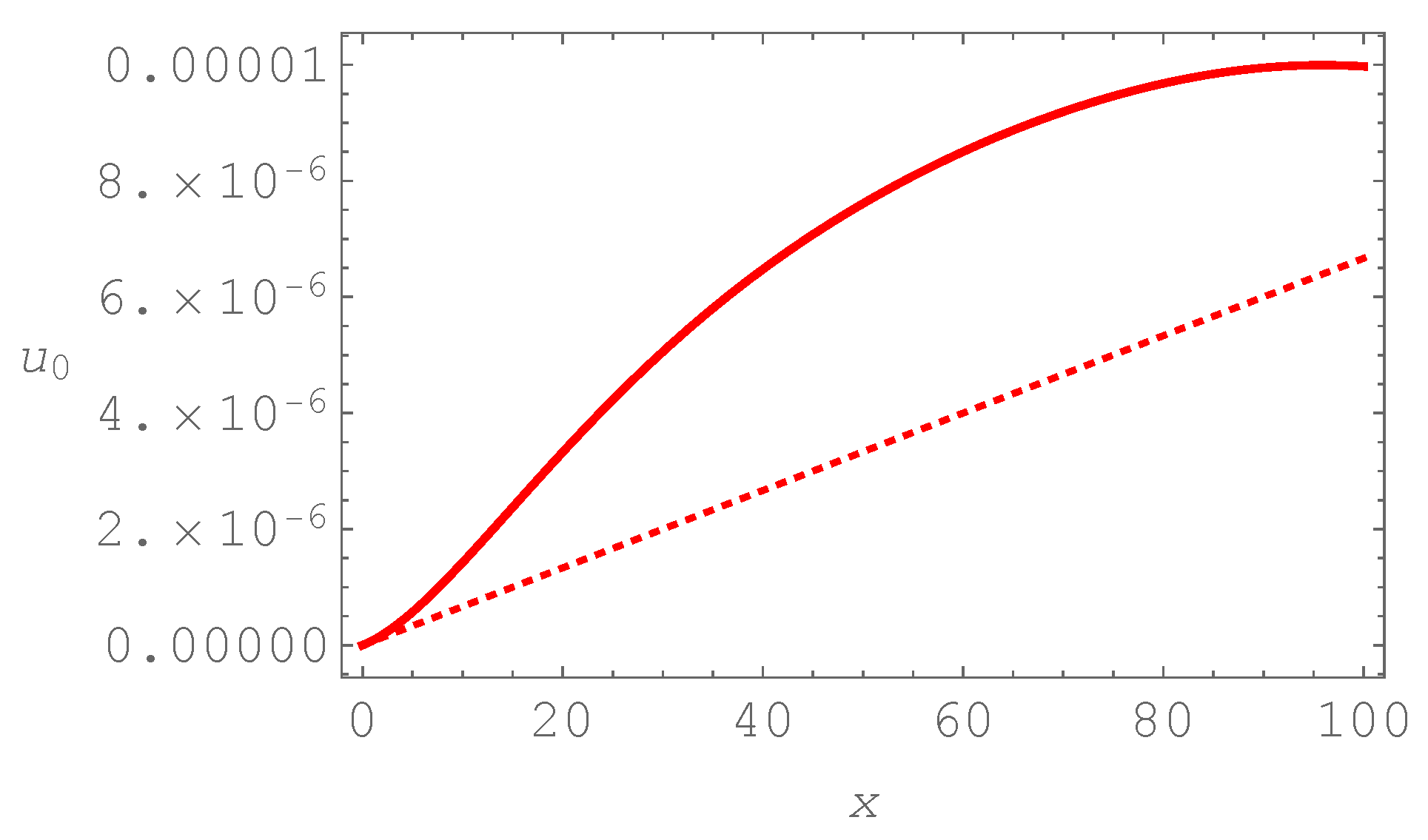
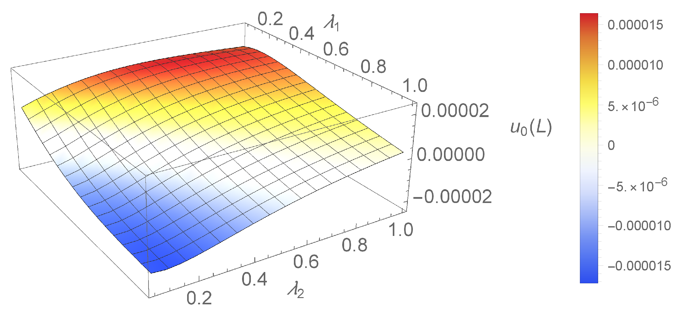
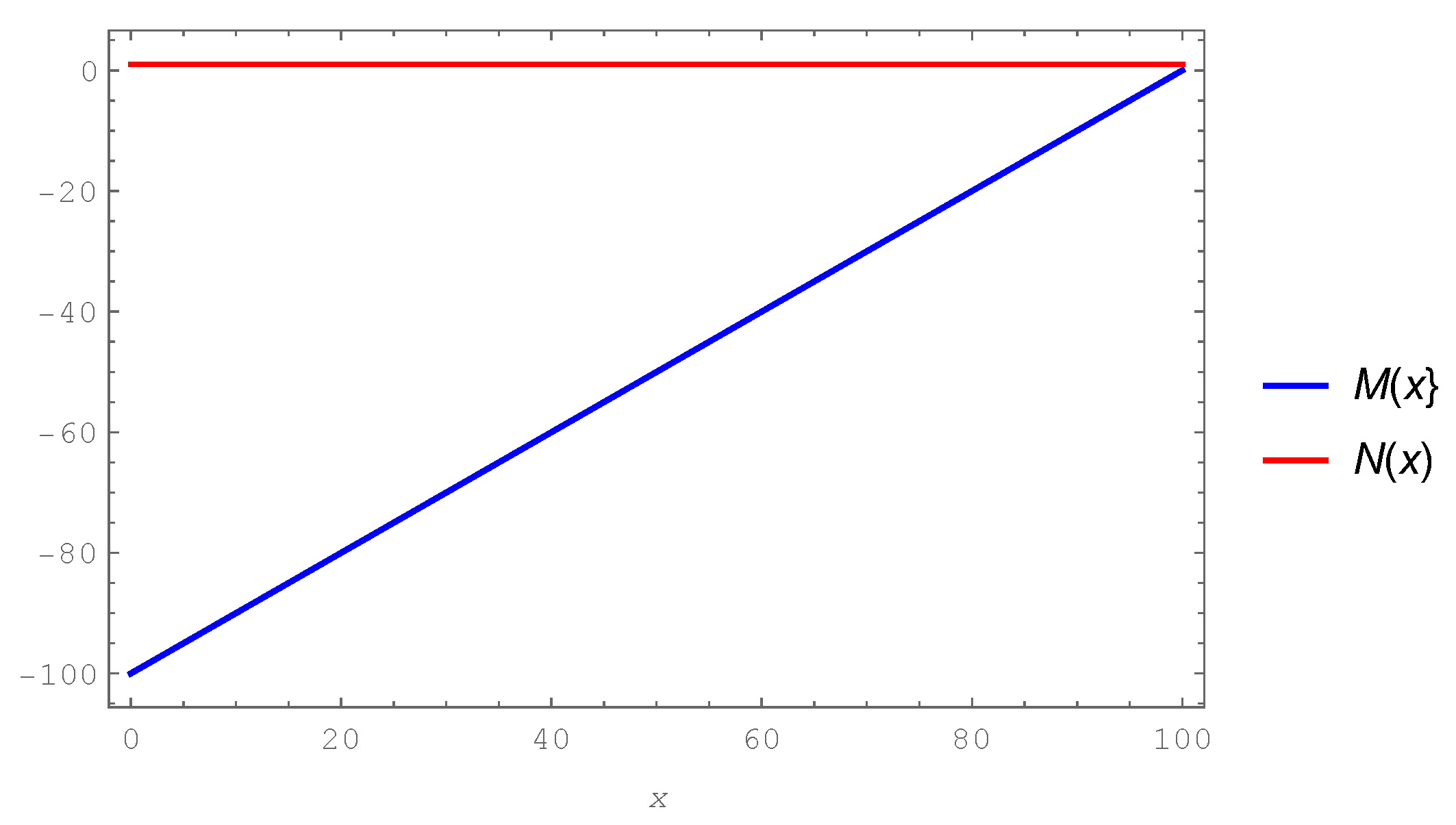
The problem was solved by the aid of Wolfram Mathematica software. The specific form of the function describing the axial displacement is too long to be presented here in detail. Instead, the graphical representation is provided in Figure 2. It is well known that the local formulation exhibits linear behavior. In the nonlocal formulation marked curvature is observed providing a nonlinear distribution. Similar effects are noted elsewhere [50,51] in the presence of thermal effects. If the nonlocal parameters are allowed to vary, the obtained surface describing the maximal elongation of the beam can be graphically presented (Figure 3). Smaller values of nonlocal parameters lead toward steep surface’s gradients, but as the nonlocal parameters are increased the effect diminishes. Interestingly, for a certain choice of nonlocal parameters average axial displacements, take negative values, although the nanobeam is loaded by the tensile axial force. This is a direct consequence of coupling terms associated to and the neutral surface shift. Finally, the distribution of the normal force along the beam nN is constant as expected (Figure 4).
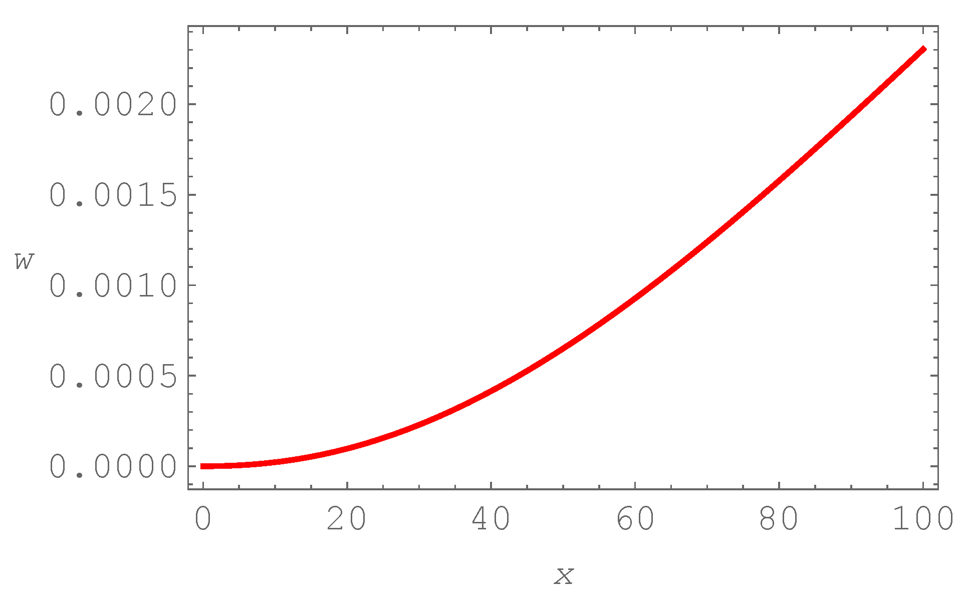
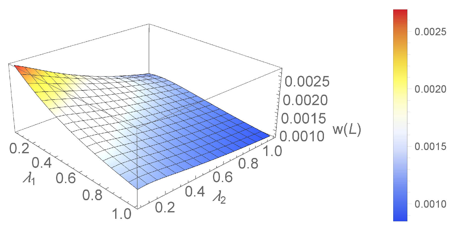
The curve representing the deformed shape of the beam for given nonlocal parameters is provided in Figure 5. The expected shape is obtained. The maximal transverse displacement at the beam’s tip for different values of the nonlocal parameters is given in Figure 6. Similar conclusions about gradients as in the case of longitudinal displacement can be drawn. The bending moment is distributed linearly along the beam (Figure 4). The moment is recovered in the post-processing from Equation (22) as nN nm.
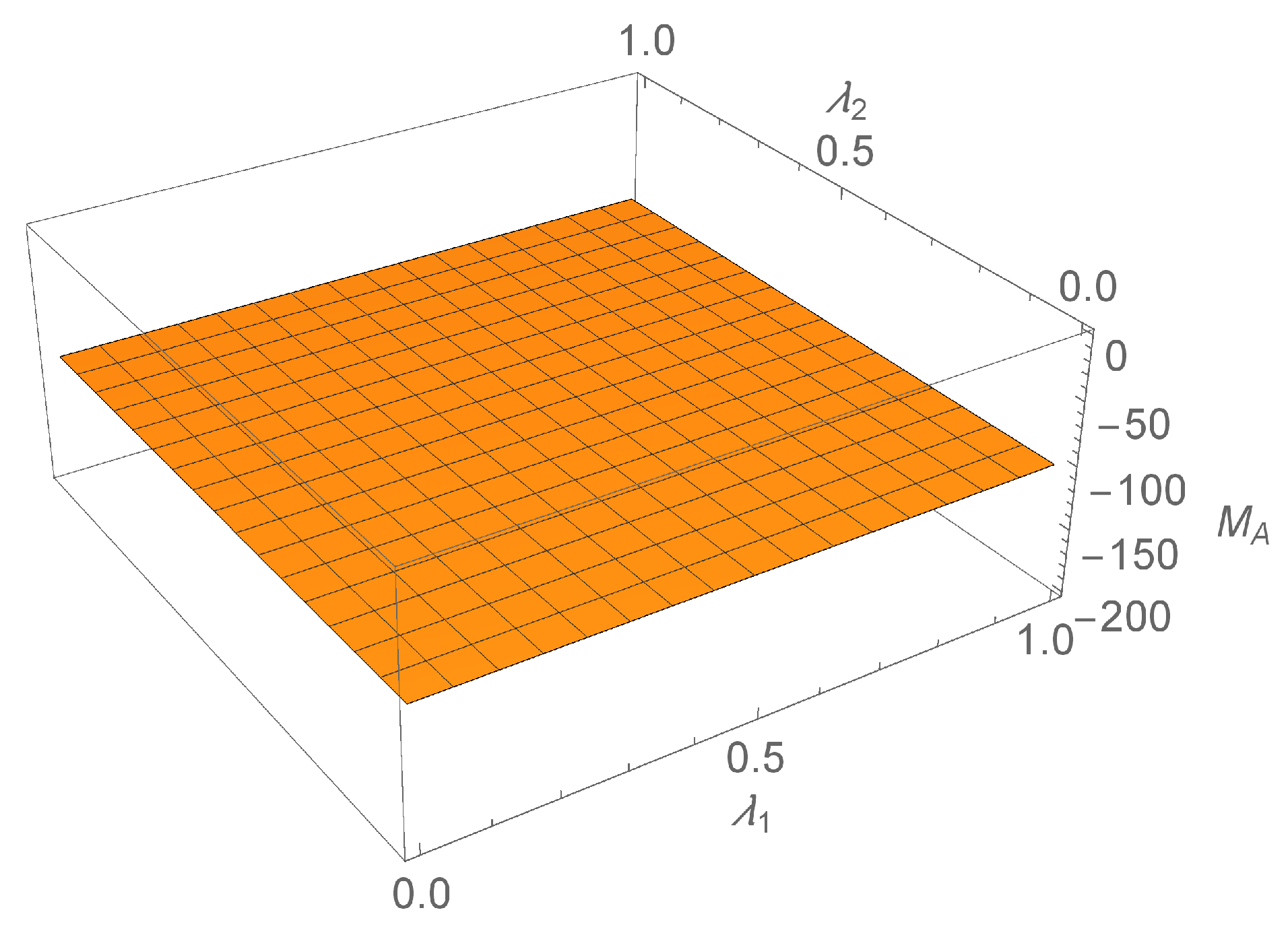
Statically determined problems, such as this one, show no dependence of support reactions on the nonlocal parameters (Figure 7).
5.2. Doubly Clamped Beam
The second example presents a statically indeterminate problem. A doubly clamped beam nm long is subjected to longitudinal constant distributed loading nN/nm and distributed transversal loading nN/nm. The beam is assembled of three layers. The first and third layers have identical geometrical and material properties. These data are provided below:
Consequently, z coordinates defining the beginning and the end of each layer are:
The beam’s cross-section is geometrically symmetric with respect to both and plane as well as with respect to material properties, thus and . With these data, the decoupled differential formulation of the problem can be set. Again, according to Table 2, the governing differential equation to be solved for the axial displacements is:
The boundary conditions are:
The constitutive boundary conditions are:
As for the bending problem, the corresponding differential framework is:
augmented with the following boundary conditions:
and constitutive boundary conditions:
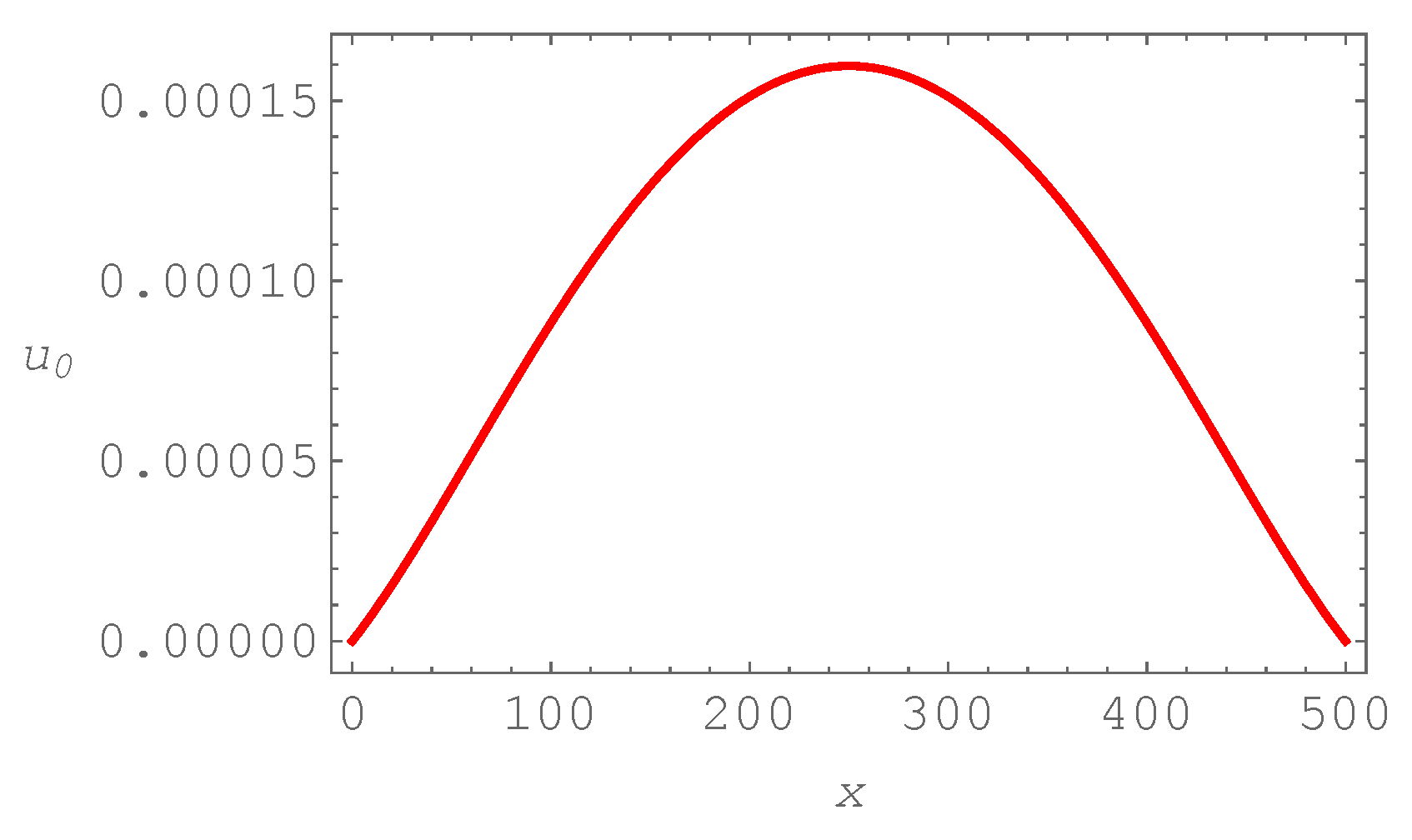
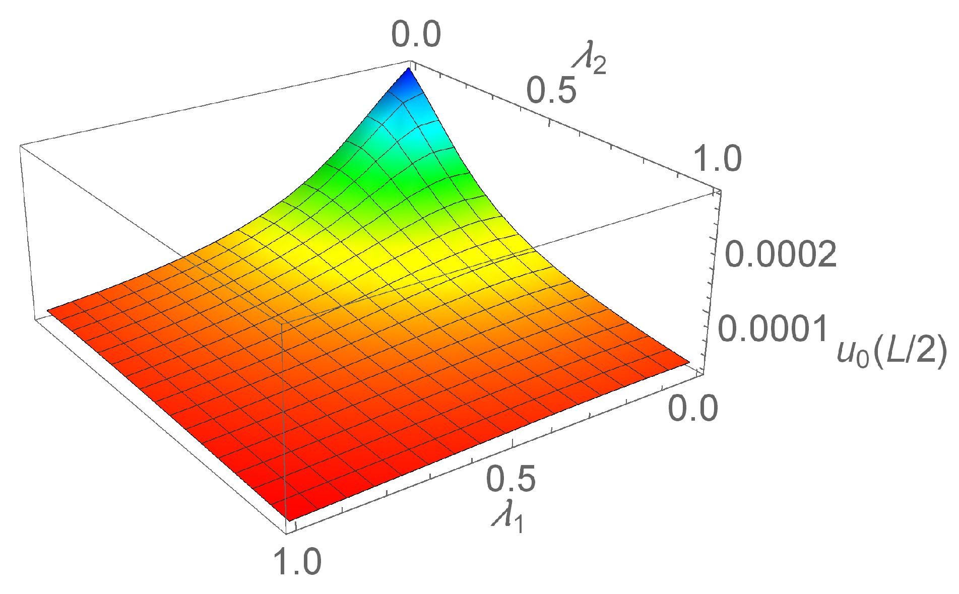
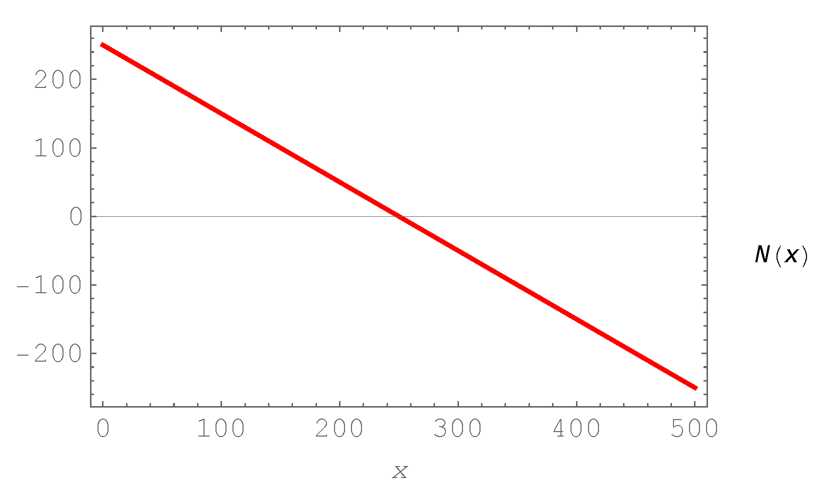
The distribution of the axial displacement along the beam is given in Figure 8. The middle point of the beam () experiences the largest displacement, while the ends fulfill prescribed boundary conditions. Next, the movement of the middle point is analyzed for dependence on the nonlocal parameters (Figure 9). The increase in either nonlocal parameter does lead toward maximal axial displacement converging toward a limit value. The linear distribution of the normal force along the beam is defined as nN (Figure 10). Support reactions are obtained as nN and nN.
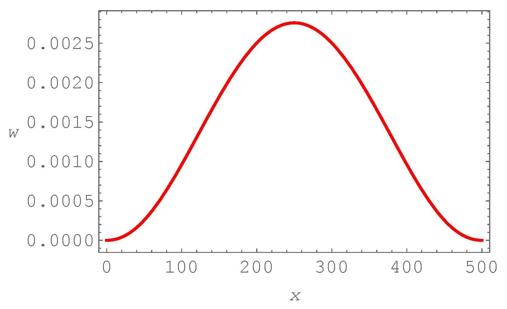
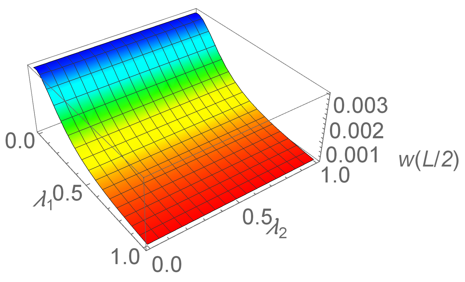
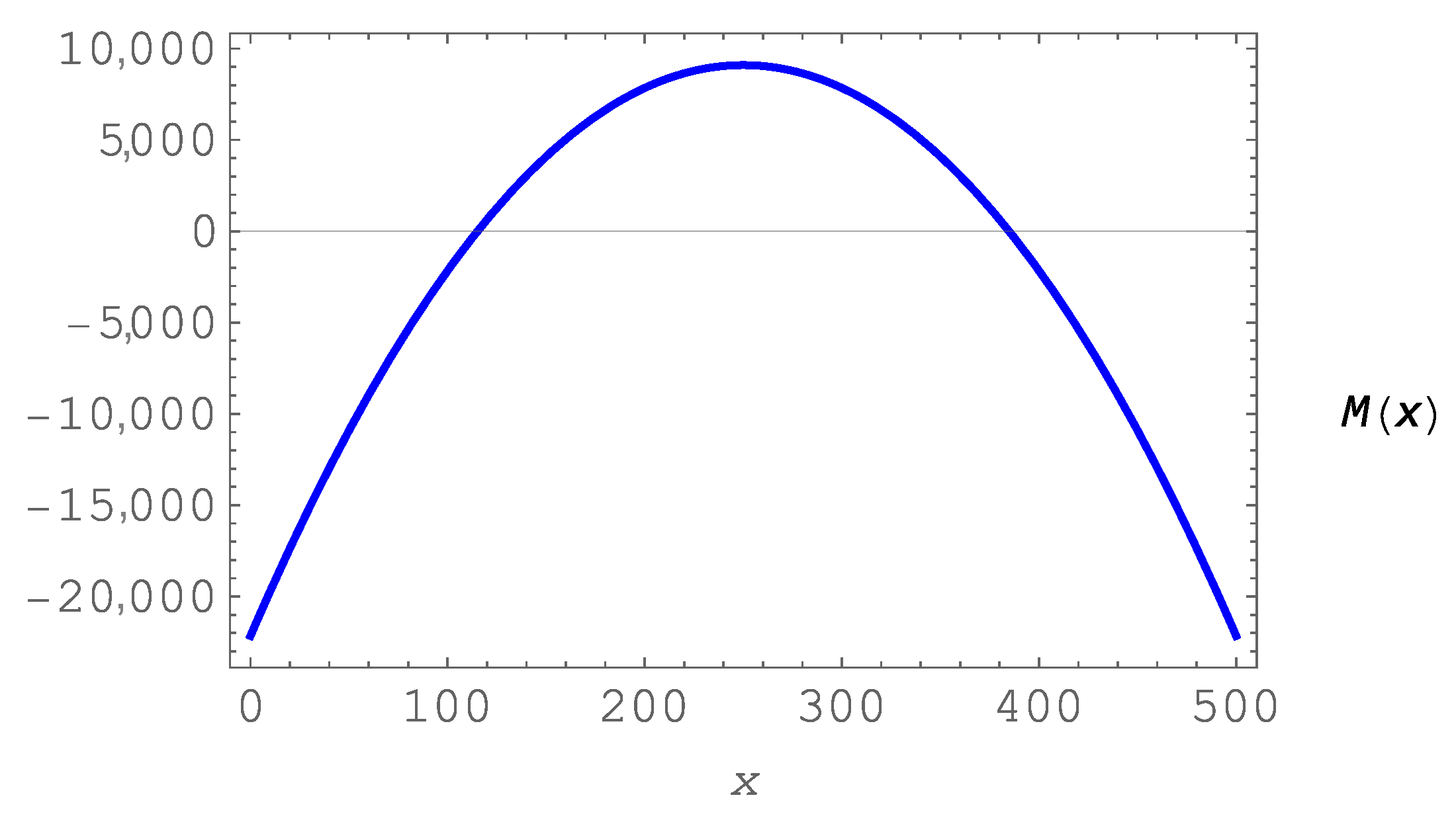
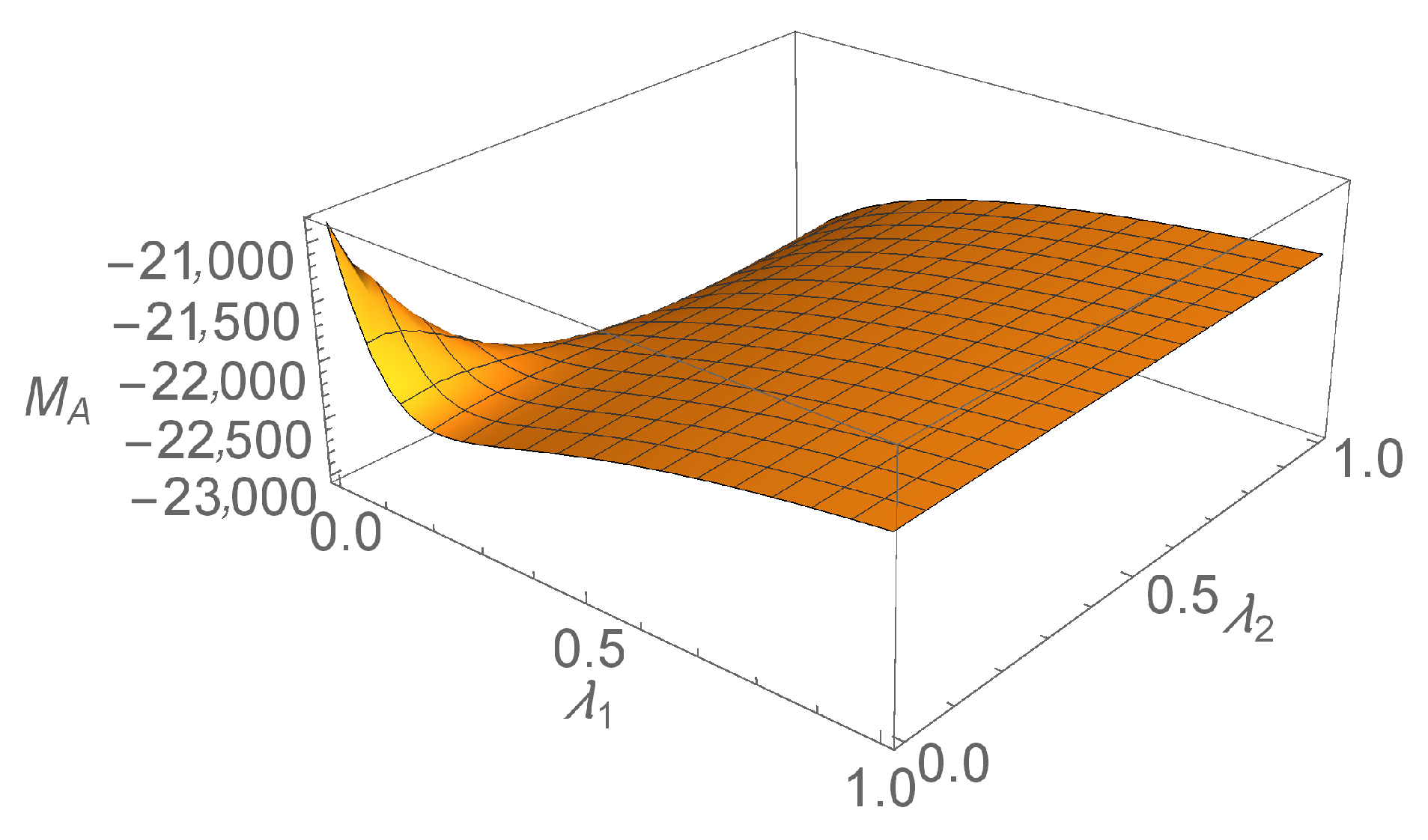
The bell-shaped curve represents the deformed shape of the beam due to bending (Figure 11). The maximal transverse displacement takes place at the middle of the beam as expected. Influence of the nonlocal parameters is given in Figure 12. Higher gradients are obtained for lower values of the nonlocal parameter compared to . The bending moment distribution in Equation (22) is defined by the parabolic polynomial (Figure 13), giving nN nm with the maximum nN nm at nm. In addition, contrary to the previous example, in the statically indeterminate problems, support reactions do depend on the nonlocal parameters (Figure 14).
6. Conclusions
The following main results of the presented research are summarized below.
- The stress-driven integral approach based on Bernoulli–Euler kinematical hypotheses is extended to composite beams assembled of multiple layers, not necessarily of equal width. As demonstrated in the examples, the approach does not suffer from paradoxes present in some other formulations.
- The more standard approach that includes mixed boundary conditions, i.e., both stress resultants and prescribed displacements, is replaced by the purely kinematical framework. In this way, it is not necessary to explicitly determine support reactions in order to calculate displacements. Support reactions and stress resultant distributions are conveniently calculated in the post-processing phase.
- The example section demonstrates that in statically undetermined structural problems, reaction systems exhibit technically significant size effects which therefore have to be taken in due account in design and optimization of a wide variety of new-generation sensors and actuators.
- In the general case of layered beams, the resulting formulation exhibits coupling between axial and transverse displacements. This gives rise to unusual nonlocal phenomena, such as shortening of the nanobeam in the presence of tensile axial force. Coupling of axial and bending terms in the governing differential equations, as well as the neutral surface shift, give rise to such effects.
- Finally, as discussed in the Introduction, if the beams with larger length/thickness ratios are to be considered, one must be wary about the surface and interface effects. An extension with a specialized size-dependent model is recommended in such cases.
Author Contributions
Conceptualization, Methodology, Software, Validation, Investigation, and Writing—Review and Editing, R.B., M.Č., and F.M.d.S. All authors contributed equally to this work. All authors have read and agreed to the published version of the manuscript.
Funding
This research received no external funding.
Acknowledgments
This work was supported in part by Croatian Science Foundation under the project IP-2019-04-4703 and by the the Italian Ministry for University and Research (P.R.I.N. National Grant 2017, Project code 2017J4EAYB; University of Naples Federico II Research Unit). This support is gratefully acknowledged.
Conflicts of Interest
The authors declare no conflict of interest.
References
- Farajpour, A.; Ghayesh, M.H.; Farokhi, H. A review on the mechanics of nanostructures. Int. J. Eng. Sci. 2018, 133, 231–263. [Google Scholar] [CrossRef]
- Pourasghar, A.; Chen, Z. Effect of hyperbolic heat conduction on the linear and nonlinear vibration of CNT reinforced size-dependent functionally graded microbeams. Int. J. Eng. Sci. 2019, 137, 57–72. [Google Scholar] [CrossRef]
- Xia, X.; Weng, G.J.; Hou, D.; Wen, W. Tailoring the frequency-dependent electrical conductivity and dielectric permittivity of CNT-polymer nanocomposites with nanosized particles. Int. J. Eng. Sci. 2019, 142, 1–19. [Google Scholar] [CrossRef]
- Mojahedi, M. Size dependent dynamic behavior of electrostatically actuated microbridges. Int. J. Eng. Sci. 2017, 111, 74–85. [Google Scholar] [CrossRef]
- Moradweysi, P.; Ansari, R.; Hosseini, K.; Sadeghi, F. Application of modified Adomian decomposition method to pull-in instability of nano-switches using nonlocal Timoshenko beam theory. Appl. Math. Model. 2018, 54, 594–604. [Google Scholar] [CrossRef]
- Hosseini, S.M. Analytical solution for nonlocal coupled thermoelasticity analysis in a heat-affected MEMS/NEMS beam resonator based on Green–Naghdi theory. Appl. Math. Model. 2018, 57, 21–36. [Google Scholar] [CrossRef]
- Tran, N.; Ghayesh, M.H.; Arjomandi, M. Ambient vibration energy harvesters: A review on nonlinear techniques for performance enhancement. Int. J. Eng. Sci. 2018, 127, 162–185. [Google Scholar] [CrossRef]
- Basutkar, R. Analytical modelling of a nanoscale series-connected bimorph piezoelectric energy harvester incorporating the flexoelectric effect. Int. J. Eng. Sci. 2019, 139, 42–61. [Google Scholar] [CrossRef]
- Ghayesh, M.H.; Farokhi, H. Nonlinear broadband performance of energy harvesters. Int. J. Eng. Sci. 2020, 147, 103202. [Google Scholar] [CrossRef]
- Sadeghian, H.; Yang, C.K.; Goosen, J.F.L.; van der Drift, E.; Bossche, A.; French, P.J.; van Keulen, F. Characterizing size-dependent effective elastic modulus of silicon nanocantilevers using electrostatic pull-in instability. Appl. Phys. Lett. 2009, 94, 221903. [Google Scholar] [CrossRef]
- Poelma, R.; Sadeghian, H.; Noijen, S.; Zaal, J.; Zhang, G. Multi-scale numerical-experimental method to determine the size dependent elastic properties of bilayer silicon copper nanocantilevers using an electrostatic pull in experiment. In Proceedings of the 2010 11th International Thermal, Mechanical & Multi-Physics Simulation, and Experiments in Microelectronics and Microsystems (EuroSimE), Bordeaux, France, 26–28 April 2010. [Google Scholar] [CrossRef]
- Sadeghian, H.; Goosen, H.; Bossche, A.; Thijsse, B.; Van Keulen, F. On the size-dependent elasticity of silicon nanocantilevers: Impact of defects. J. Phys. Appl. Phys. 2011, 44. [Google Scholar] [CrossRef] [Green Version]
- Li, C.; Chou, T.W. A structural mechanics approach for the analysis of carbon nanotubes. Int. J. Solids Struct. 2003, 40, 2487–2499. [Google Scholar] [CrossRef]
- Li, C.; Chou, T. Elastic moduli of multi-walled Carbon nanotubes and the effect of van der Waals forces. Compos. Sci. Technol. 2003, 63, 1517–1524. [Google Scholar] [CrossRef]
- Barretta, R.; Brcic, M.; Canadija, M.; Luciano, R.; de Sciarra, F.M. Application of gradient elasticity to armchair carbon nanotubes: Size effects and constitutive parameters assessment. Eur. J. Mech. A Solids 2017, 65, 1–13. [Google Scholar] [CrossRef]
- Preethi, K.; Raghu, P.; Rajagopal, A.; Reddy, J. Nonlocal nonlinear bending and free vibration analysis of a rotating laminated nano cantilever beam. Mech. Adv. Mater. Struct. 2018, 25, 439–450. [Google Scholar] [CrossRef]
- Arefi, M.; Zenkour, A. Size-dependent vibration and bending analyses of the piezomagnetic three-layer nanobeams. Appl. Phys. Mater. Sci. Process. 2017, 123. [Google Scholar] [CrossRef]
- Arefi, M.; Zenkour, A. Influence of magneto-electric environments on size-dependent bending results of three-layer piezomagnetic curved nanobeam based on sinusoidal shear deformation theory. J. Sandw. Struct. Mater. 2019, 21, 2751–2778. [Google Scholar] [CrossRef]
- Wang, Q.; Mao, D.; Zhu, J.; Dong, L. NEMS-based asymmetric split ring resonators for thermomechanically tunable infrared metamaterials. In Proceedings of the 2017 IEEE 17th International Conference on Nanotechnology (IEEE-NANO), Pittsburgh, PA, USA, 25–28 July 2017; pp. 834–837. [Google Scholar] [CrossRef]
- Feng, L.; Gao, F.; Liu, M.; Wang, S.; Li, L.; Shen, M.; Wang, Z. Investigation of the mechanical bending and frequency shift induced by adsorption and temperature using micro- and nanocantilever sensors. J. Appl. Phys. 2012, 112, 013501. [Google Scholar] [CrossRef]
- Xu, M.; Wang, B.; Yu, A. Effects of surface energy on the nonlinear behaviors of laminated nanobeams. Int. J. Precis. Eng. Manuf. Green Technol. 2017, 4, 105–111. [Google Scholar] [CrossRef]
- Müller, P.; Saúl, A. Elastic effects on surface physics. Surf. Sci. Rep. 2004, 54, 157–258. [Google Scholar] [CrossRef]
- Miller, R.E.; Shenoy, V.B. Size-dependent elastic properties of nanosized structural elements. Nanotechnology 2000, 11, 139. [Google Scholar] [CrossRef]
- Rongong, J.; Goruppa, A.; Buravalla, V.; Tomlinson, G.; Jones, F. Plasma deposition of constrained layer damping coatings. Proc. Inst. Mech. Eng. Part J. Mech. Eng. Sci. 2004, 218, 669–680. [Google Scholar] [CrossRef] [Green Version]
- Catania, G.; Strozzi, M. Damping oriented design of thin-walled mechanical components by means of multi-layer coating technology. Coatings 2018, 8, 73. [Google Scholar] [CrossRef] [Green Version]
- Yu, L.; Ma, Y.; Zhou, C.; Xu, H. Damping efficiency of the coating structure. Int. J. Solids Struct. 2005, 42, 3045–3058. [Google Scholar] [CrossRef]
- Eringen, A. On differential equations of nonlocal elasticity and solutions of screw dislocation and surface waves. J. Appl. Phys. 1983, 54, 4703–4710. [Google Scholar] [CrossRef]
- Romano, G.; Barretta, R.; Diaco, M.; Marotti de Sciarra, F. Constitutive boundary conditions and paradoxes in nonlocal elastic nanobeams. Int. J. Mech. Sci. 2017, 121, 151–156. [Google Scholar] [CrossRef]
- Romano, G.; Barretta, R. Stress-driven versus strain-driven nonlocal integral model for elastic nano-beams. Compos. Part Eng. 2017, 114, 184–188. [Google Scholar] [CrossRef]
- Challamel, N.; Wang, C. The small length scale effect for a non-local cantilever beam: A paradox solved. Nanotechnology 2008, 19, 345703. [Google Scholar] [CrossRef]
- Peddieson, J.; Buchanan, G.R.; McNitt, R.P. Application of nonlocal continuum models to nanotechnology. Int. J. Eng. Sci. 2003, 41, 305–312. [Google Scholar] [CrossRef]
- Romano, G.; Barretta, R. Nonlocal elasticity in nanobeams: The stress-driven integral model. Int. J. Eng. Sci. 2017, 115, 14–27. [Google Scholar] [CrossRef]
- Uvarov, I.; Naumov, V.; Amirov, I. Resonance properties of multilayer metallic nanocantilevers. In Proceedings of the International Conference Micro-and Nano-Electronics 2012, Zvenigorod, Russia, 1–5 October 2012; Volume 8700. [Google Scholar] [CrossRef]
- Barretta, R.; Čanađija, M.; de Sciarra, F.M. Nonlocal integral thermoelasticity: A thermodynamic framework for functionally graded beams. Compos. Struct. 2019, 225, 111104. [Google Scholar] [CrossRef] [Green Version]
- Dehrouyeh-Semnani, A.M. On boundary conditions for thermally loaded FG beams. Int. J. Eng. Sci. 2017, 119, 109–127. [Google Scholar] [CrossRef]
- Larbi, L.O.; Kaci, A.; Houari, M.S.A.; Tounsi, A. An efficient shear deformation beam theory based on neutral surface position for bending and free vibration of functionally graded beams. Mech. Based Des. Struct. Mach. 2013, 41, 421–433. [Google Scholar] [CrossRef]
- Abu Al-Rub, R.; Voyiadjis, G. Analytical and experimental determination of the material intrinsic length scale of strain gradient plasticity theory from micro- and nano-indentation experiments. Int. J. Plast. 2004, 20, 1139–1182. [Google Scholar] [CrossRef]
- Perkins, R.W., Jr.; Thompson, D. Experimental evidence of a couple-stress effect. AIAA J. 1973, 11, 1053–1055. [Google Scholar] [CrossRef]
- Kakunai, S.; Masaki, J.; Kuroda, R.; Iwata, K.; Nagata, R. Measurement of apparent Young’s modulus in the bending of cantilever beam by heterodyne holographic interferometry. Exp. Mech. 1985, 25, 408–412. [Google Scholar] [CrossRef]
- Zhang, Y.; Wang, C.; Tan, V. Assessment of Timoshenko beam models for vibrational behavior of single-walled carbon nanotubes using molecular dynamics. Adv. Appl. Math. Mech. 2009, 1, 89–106. [Google Scholar]
- Arash, B.; Ansari, R. Evaluation of nonlocal parameter in the vibrations of single-walled carbon nanotubes with initial strain. Physica E 2010, 42, 2058–2064. [Google Scholar] [CrossRef]
- Narendar, S.; Gopalakrishnan, S. Critical buckling temperature of single-walled carbon nanotubes embedded in a one-parameter elastic medium based on nonlocal continuum mechanics. Physica E 2011, 43, 1185–1191. [Google Scholar] [CrossRef]
- Duan, W.; Wang, C.; Zhang, Y. Calibration of nonlocal scaling effect parameter for free vibration of carbon nanotubes by molecular dynamics. J. Appl. Phys. 2007, 101, 024305. [Google Scholar] [CrossRef]
- Xiao, S.; Hou, W. Studies of size effects on carbon nanotubes’ mechanical properties by using different potential functions. Fuller. Nanotub. Carbon Nanostruct. 2006, 14, 9–16. [Google Scholar] [CrossRef]
- Polyanin, A.D.; Manzhirov, A.V. Handbook of Integral Equations; CRC: Boca Raton, FL, USA, 1998. [Google Scholar]
- Barretta, R.; Čanađija, M.; Luciano, R.; de Sciarra, F.M. Stress-driven modeling of nonlocal thermoelastic behavior of nanobeams. Int. J. Eng. Sci. 2018, 126, 53–67. [Google Scholar] [CrossRef] [Green Version]
- Barretta, R.; Luciano, R.; de Sciarra, F.M.; Ruta, G. Stress-driven nonlocal integral model for Timoshenko elastic nano-beams. Eur. J. Mech. A Solids 2018, 72, 275–286. [Google Scholar] [CrossRef]
- Barretta, R.; Fabbrocino, F.; Luciano, R.; de Sciarra, F.M. Closed-form solutions in stress-driven two-phase integral elasticity for bending of functionally graded nano-beams. Physica E 2018, 97, 13–30. [Google Scholar] [CrossRef]
- Barretta, R.; Canadija, M.; Marotti de Sciarra, F. Modified Nonlocal Strain Gradient Elasticity for Nano-Rods and Application to Carbon Nanotubes. Appl. Sci. 2019, 9, 514. [Google Scholar] [CrossRef] [Green Version]
- Canadija, M.; Barretta, R.; Marotti de Sciarra, F. A gradient elasticity model of Bernoulli-Euler nanobeams in non-isothermal environments. Eur. J. Mech. A Solids 2016, 55, 243–255. [Google Scholar] [CrossRef]
- Canadija, M.; Barretta, R.; Marotti de Sciarra, F. On functionally graded Timoshenko nonisothermal nanobeams. Compos. Struct. 2016, 135, 286–296. [Google Scholar] [CrossRef]
Figure 1.
Cross-section and stress resultants of a layered nonlocal beam.

Figure 2.
Axial displacement (nm) of the beam loaded with the longitudinal force at the free end, (continuous line) and local solution (dotted line), x (nm).
Figure 2.
Axial displacement (nm) of the beam loaded with the longitudinal force at the free end, (continuous line) and local solution (dotted line), x (nm).

Figure 3.
Three-dimensional representation of the free end’s longitudinal displacement (nm) for different values of nonlocal parameters.
Figure 3.
Three-dimensional representation of the free end’s longitudinal displacement (nm) for different values of nonlocal parameters.

Figure 4.
Distribution of the normal force (nN) and bending moment (nN nm) along the cantilever beam, x (nm).
Figure 4.
Distribution of the normal force (nN) and bending moment (nN nm) along the cantilever beam, x (nm).

Figure 5.
Transverse displacement (nm) of the beam loaded with the transverse force at the free end, , x (nm).
Figure 5.
Transverse displacement (nm) of the beam loaded with the transverse force at the free end, , x (nm).

Figure 6.
Three-dimensional representation of the free end’s transverse displacement (nm) for different values of nonlocal parameters.
Figure 6.
Three-dimensional representation of the free end’s transverse displacement (nm) for different values of nonlocal parameters.

Figure 7.
Support reaction (nN nm) is independent of nonlocal parameters.

Figure 8.
The longitudinal displacement (nm) of a doubly clamped beam, x (nm).

Figure 9.
Three-dimensional representation of the beam’s middle axial displacement (nm) for different values of nonlocal parameters, .
Figure 9.
Three-dimensional representation of the beam’s middle axial displacement (nm) for different values of nonlocal parameters, .

Figure 10.
Distribution of the normal force (nN) along the doubly clamped beam, x (nm).

Figure 11.
The transverse displacement (nm) and x (nm).

Figure 12.
Three-dimensional representation of the beam’s middle transverse displacement (nm) for different values of nonlocal parameters, .
Figure 12.
Three-dimensional representation of the beam’s middle transverse displacement (nm) for different values of nonlocal parameters, .

Figure 13.
Bending moment (nN nm) in the doubly clamped beam, x (nm).

Figure 14.
Support reaction (nN nm) in the doubly clamped beam in terms of nonlocal parameters.


Table 1.
Coupled nonlocal layered beams framework for beams with symmetry of the cross-section, .
| Calculate stiffnesses: | , | |
| , | ||
| Coupled formulation: | , | |
| . | ||
| Boundary conditions: | ||
| Constitutive boundary | ||
| conditions: | ||
Table 2.
Decoupled nonlocal layered beams framework for beams with material and geometric symmetry of the cross-section, and .
Table 2.
Decoupled nonlocal layered beams framework for beams with material and geometric symmetry of the cross-section, and .
| Calculate stiffnesses: | , | |
| , | ||
| Axial displacements: | ||
| Constitutive boundary | ||
| conditions: | ||
| Boundary conditions: | ||
| Transverse displacements: | ||
| Constitutive boundary | ||
| conditions: | ||
| Boundary conditions: | ||
© 2020 by the authors. Licensee MDPI, Basel, Switzerland. This article is an open access article distributed under the terms and conditions of the Creative Commons Attribution (CC BY) license (http://creativecommons.org/licenses/by/4.0/).
Share and Cite
MDPI and ACS Style
Barretta, R.; Čanađija, M.; Marotti de Sciarra, F. Nonlocal Mechanical Behavior of Layered Nanobeams. Symmetry 2020, 12, 717. https://doi.org/10.3390/sym12050717
AMA Style
Barretta R, Čanađija M, Marotti de Sciarra F. Nonlocal Mechanical Behavior of Layered Nanobeams. Symmetry. 2020; 12(5):717. https://doi.org/10.3390/sym12050717
Chicago/Turabian StyleBarretta, Raffaele, Marko Čanađija, and Francesco Marotti de Sciarra. 2020. "Nonlocal Mechanical Behavior of Layered Nanobeams" Symmetry 12, no. 5: 717. https://doi.org/10.3390/sym12050717
Note that from the first issue of 2016, this journal uses article numbers instead of page numbers. See further details here.