An Eigenvalues Approach for a Two-Dimensional Porous Medium Based Upon Weak, Normal and Strong Thermal Conductivities

Abstract

This work is devoted to the investigation of a two-dimensional porous material under weak, strong and normal conductivity, using the eigenvalues method. By using Laplace–Fourier transformations with the eigenvalues technique, the variables are analytically obtained. The derived technique is assessed with numerical results that are obtained from the porous mediums using simplified symmetric geometry. The results, including the displacements, temperature, stresses and the change in the volume fraction field, are offered graphically. Comparisons are made among the outcomes obtained under weak, normal and strong conductivity.

1. Introduction

Porous mediums appear in a wide variety of forms in the environment, and can be natural or synthetically produced, with several implementations in technology. To overcome the first shortage of the uncoupled thermo-elasticity theory, in 1956, Biot [1] presented the model of coupled thermo-elasticity to overcome the first shortage using the theory of decoupled thermo-elasticity, where it prognosticates two phenomena not appropriate for physical observation. First, the thermal equation is parabolic, predicting infinite propagation velocities for heatwaves. Second, the thermal conduction equation of this model contains no elastic term. In Biot’s theory, the governing equations are coupled, eliminating the second paradox of uncoupled theory. But the thermal equation is also parabolic for the coupled theory. By postulating a new thermal conduction law replacing the classical Fourier law, the generalized thermo-elastic model at thermal delay times was confirmed by [2].

The generalizations of the concepts of derivatives and integrals regarding a nonintegral order have been the subject of various methods, and numerous alternative definitions of the fractional derivative have emerged. By using fractional calculation, several real models of physical proceedings have been successfully amended. It can be said with certainty that all integration models and fractional derivatives were formed in the second half of the 20th century. Furthermore, various methods and definitions of fractional derivatives have become the main object of several investigates. In the context of generalized thermo-elastic theories, Youssef, Youssef and Al-Lehaibi [3,4] have presented the generalized fractional-order thermo-elastic model under weak, normal and strong thermal conductivities. Based on Taylor’s expansions of time-fractional orders, Ezzat and El Karamany [5] have given other models for fractional orders and generalized thermoelastic theories. A new theory is presented by the heat conduction law, as in Sherief et al. [6].

The models of elastic materials containing voids are one of the ultimate considerable generalizations of the classical elastic models. This theorem points to elastic materials that contain small holes, in which the empty volume is inclusive between the kinematic variables. In practice, these models are beneficial for studying many types of geological and biological media for which the elastic models are ineligible. Karageorghis et al. [7] have studied the movable pseudo-boundary for voids detection in a two-dimension thermoelastic medium. Singh [8] investigated the propagation of wave in porous media in the context of the generalized thermo-elasticity theory. Marin et al. [9] have presented the solutions to several problems for dipolar elastic bodies. Sarkar [10] has applied the time-fractional order, two-temperatures model to investigate the wave propagation in initially stressed elastic plane solids under a magneto–thermo-elasticity model. Ezatt et al. [11] presented modeling regarding generalized thermo-elasticity, based on the memory-dependent derivative. Several authors [12,13,14,15,16,17,18] have solved several problems under generalized theories of thermo-elasticity. Ellahi et al. [19,20] have presented the solutions to some problems under various boundary conditions in porous mediums. Many researchers [21,22,23,24,25,26,27,28,29] studied thermal conductivities by using the fractional thermo-elastic model. In the domain of Laplace, the eigenvalues method gave exact solutions without any presupposed restrictions on actual physical quantities.

This article aims to study the effects of weak, normal and strong thermal conductivity in two-dimension porous media using the eigenvalue technique. By using the eigenvalues method and Laplace and Fourier transformations, based on numerical and analytical approaches, the governing relations are treated. For all variables, the numerical outcomes are obtained and offered graphically. Comparisons are made among the outcomes obtained under weak, normal and strong thermal conductivity.

2. Mathematical Model

For a homogeneous and isotropic two-dimensional elastic media with voids, the governing relations in the context of the generalized thermoelastic theory [3], based on [8], in the absence of body force and the thermal sources can be introduced by

$$\left(\lambda +\mu \right)u_{j,ij}+\mu u_{i,jj}+b{\phi }_{,i}-{\gamma }_t{\mathsf{\Theta }}_{,i}=\rho \frac{{\partial }^2{u}_i}{\partial t^2}$$

(1)

$$\alpha {\phi }_{,jj}-b{u}_{j,j}-{\zeta }_1\phi -{\omega }_o\frac{\partial \phi }{\partial t}+m\mathsf{\Theta }=\rho \psi \frac{{\partial }^2\phi }{\partial t^2}$$

(2)

$${\left(K{I}^{ϵ-1}{\mathsf{\Theta }}_{,j}\right)}_{,j}=\left(1+{\tau }_o\frac{\partial }{\partial t}\right)\left(\rho c_e\frac{\partial \mathsf{\Theta }}{\partial t}+m{T}_o\frac{\partial \phi }{\partial t}+{\gamma }_t{T}_o\frac{\partial u_{j,j}}{\partial t}\right), 0<ϵ\le 2.$$

(3)

where the fractional integral operator can be defined by

$$I^{ϵ-1}g\left(\mathit{r},t\right)=\frac{1}{\mathsf{\Gamma }(\in )}\underset{0}{\overset{t}{\int }}{\left(t-\tau \right)}^{ϵ-1}g\left(\mathit{r},\tau \right)d\tau , \{\begin{array}{cc}0<ϵ<1,& weak conductivity\\ ϵ=1,& normal conductivity\\ 1<ϵ\le 2,& strong conductivity\end{array}$$

(4)

with the Gamma function $\mathsf{\Gamma }(\in )$.

The stress-displacement symmetric relations can be given as

$${\sigma }_{ij}=\mu \left(u_{i,j}+u_{j,i}\right)+\left(\lambda u_{k,k}+b\phi -{\gamma }_t\mathsf{\Theta }\right){\delta }_{ij}$$

(5)

where ${\omega }_o, \alpha , m, b, \psi ,{\zeta }_1$ are the medium constants caused by the presence of voids; $i,j,k=1,2,3$, ${\tau }_o$ is the thermal delay time; $\rho$ is the density of the material; ${\sigma }_{ij}$ are the symmetry components of stress; $\phi$ is the change in the volume fraction of the voids;$K$ is the coefficient of thermal conductivity; $\mathsf{\Theta }=T-T_o$; $T_o$ is the reference temperature; ${\gamma }_t=\left(3\lambda +2\mu \right){\alpha }_t$ is the thermal modulus; ${\alpha }_t$ is the linear thermal expansion coefficient;$u_i$ are the displacement components; $c_e$ is the specific heat at a constant strain; $\lambda ,\mu$ are the Lame constants; and $t$ is the time.

3. Formulation of the Problem

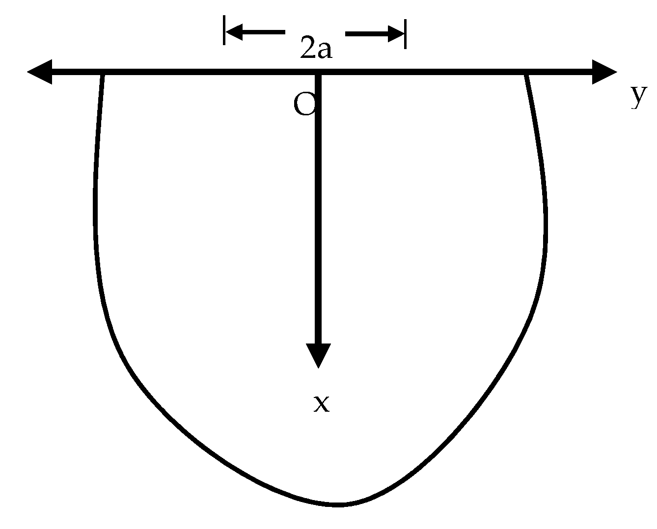
We consider that an elastic, homogenous and isotropic medium containing voids in two-dimensions fills the regions $0\le x\le \infty ,-\infty \le y\le \infty$, as in Figure 1. Based on the model of Lord and Shulman, the basic equations will be written by using the Cartesian coordinates $\left(x,y,z\right)$and the displacement components $\left(u,v,0\right)$, so

$$\left(\lambda +2\mu \right)\frac{{\partial }^{2}u}{\partial x^2}+\left(\lambda +\mu \right)\frac{{\partial }^{2}v}{\partial x\partial y}+\mu \frac{{\partial }^{2}u}{\partial y^2}+b\frac{\partial \phi }{\partial x}-{\gamma }_t\frac{\partial \mathsf{\Theta }}{\partial x}=\rho \frac{{\partial }^{2}u}{\partial t^2}$$

(6)

$$\left(\lambda +2\mu \right)\frac{{\partial }^{2}v}{\partial y^2}+\left(\lambda +\mu \right)\frac{{\partial }^{2}u}{\partial x\partial y}+\mu \frac{{\partial }^{2}v}{\partial x^2}+b\frac{\partial \phi }{\partial y}-{\gamma }_t\frac{\partial \mathsf{\Theta }}{\partial y}=\rho \frac{{\partial }^{2}v}{\partial t^2}$$

(7)

$$\alpha \left(\frac{{\partial }^2\phi }{\partial x^2}+\frac{{\partial }^2\phi }{\partial y^2}\right)-{\omega }_o\frac{\partial \phi }{\partial t}-{\zeta }_1\phi -b\left(\frac{\partial u}{\partial x}+\frac{\partial v}{\partial y}\right)+m\mathsf{\Theta }=\rho \psi \frac{{\partial }^2\phi }{\partial t^2}$$

(8)

$$K{I}^{ϵ-1}\left(\frac{{\partial }^2\mathsf{\Theta }}{\partial x^2}+\frac{{\partial }^2\mathsf{\Theta }}{\partial y^2}\right)=\left(1+{\tau }_o\frac{\partial }{\partial t}\right)\left(\rho c_e\frac{\partial \mathsf{\Theta }}{\partial t}+m{T}_o\frac{\partial \phi }{\partial t}+{\gamma }_t{T}_o\frac{\partial }{\partial t}\left(\frac{\partial u}{\partial x}+\frac{\partial v}{\partial y}\right)\right)$$

(9)

$${\sigma }_{xx}=\lambda \frac{\partial v}{\partial y}+\left(\lambda +2\mu \right)\frac{\partial u}{\partial x}+b\phi -{\gamma }_t\mathsf{\Theta }, {\sigma }_{xy}=\mu \left(\frac{\partial v}{\partial x}+\frac{\partial u}{\partial y}\right)$$

(10)

The problem initial conditions can be defined as

$$\begin{array}{c}\mathsf{\Theta }\left(x,y,0\right)=\frac{\partial \mathsf{\Theta }\left(x,y,0\right)}{\partial t}=0, \phi \left(x,y,0\right)=\frac{\partial \phi \left(x,y,0\right)}{\partial t}=0,\\ u\left(x,y,0\right)=\frac{\partial u\left(x,y,0\right)}{\partial t}=0, v\left(x,y,0\right)=\frac{\partial v\left(x,y,0\right)}{\partial t}=0\end{array}$$

(11)

While the appropriate boundary conditions can be defined by

$${\sigma }_{xx}={\sigma }_{xy}=0.0,-K\frac{\partial \mathsf{\Theta }\left(x,y,t\right)}{\partial x}=q_o\frac{t^2{e}^{-\frac{t}{t_p}}}{16t_p^2}H\left(a-\left|y\right|\right), \frac{\partial \phi }{\partial x}=0$$

(12)

where H is the Heaviside function; $q_o$ is a constant; and $t_p$ is the characteristic time of the pulse heat flux. For appropriateness, the dimensionless parameters can be defined by

$$\begin{array}{c}{\mathsf{\Theta }}^{\prime }=\frac{\mathsf{\Theta }}{T_o}, {\phi }^{\prime }=\psi {\eta }^2{c}^2\phi , \left({\sigma }_{xx}^{\prime },{\sigma }_{xy}^{\prime }\right)=\frac{\left( {\sigma }_{xx}, {\sigma }_{xy}\right)}{\left(\lambda +2\mu \right)},\\ \left(x^{\prime },y^{\prime },u^{\prime },v^{\prime }\right)=\eta c\left(x,y,u,v\right),\left(t^{\prime },{\tau }_o^{\prime }\right)=\eta c^2\left(t,{\tau }_o\right)\end{array}$$

(13)

where $\eta =\frac{\rho c_e}{k}$ and $c=\sqrt{\frac{\lambda +2\mu }{\mathsf{\rho }}}$.

In these dimensionless terms of the parameters in Equation (13), the basic equations will be reduced (the dash has been neglected for appropriateness).

$$\frac{{\partial }^{2}u}{\partial t^2}=\frac{{\partial }^{2}u}{\partial x^2}+\left(1-r_1\right)\frac{{\partial }^{2}v}{\partial x\partial y}+r_1\frac{{\partial }^{2}u}{\partial y^2}+r_2\frac{\partial \phi }{\partial x}-r_3\frac{\partial \mathsf{\Theta }}{\partial x}$$

(14)

$$\frac{{\partial }^{2}v}{\partial t^2}=\frac{{\partial }^{2}v}{\partial y^2}+\left(1-r_1\right)\frac{{\partial }^{2}u}{\partial x\partial y}+r_1\frac{{\partial }^{2}v}{\partial x^2}+r_2\frac{\partial \phi }{\partial y}-r_3\frac{\partial \mathsf{\Theta }}{\partial y}$$

(15)

$$r_4\frac{{\partial }^2\phi }{\partial t^2}=\frac{{\partial }^2\phi }{\partial x^2}+\frac{{\partial }^2\phi }{\partial y^2}-r_5\frac{\partial \phi }{\partial t}-r_6\phi -r_7\left(\frac{\partial u}{\partial x}+\frac{\partial v}{\partial y}\right)+r_8\mathsf{\Theta }$$

(16)

$$\frac{{\partial }^2\mathsf{\Theta }}{\partial x^2}+\frac{{\partial }^2\mathsf{\Theta }}{\partial y^2}=\frac{{\partial }^{ϵ}}{\partial t^{ϵ}}\left(1+{\tau }_o\frac{\partial }{\partial t}\right)\left(\mathsf{\Theta }+r_9\phi +r_{10}\left(\frac{\partial u}{\partial x}+\frac{\partial v}{\partial y}\right)\right)$$

(17)

$${\sigma }_{xx}=\left(1-2r_1\right)\frac{\partial v}{\partial y}+\frac{\partial u}{\partial x}+r_2\phi -r_3\mathsf{\Theta }, {\sigma }_{xy}=r_1\left(\frac{\partial v}{\partial x}+\frac{\partial u}{\partial y}\right)$$

(18)

$${\sigma }_{xx}={\sigma }_{xy}=0.0, \frac{\partial \mathsf{\Theta }\left(x,y,t\right)}{\partial x}=-q_o\frac{t^2{e}^{-\frac{t}{t_p}}}{16t_p^2}H\left(a-\left|y\right|\right), \frac{\partial \phi }{\partial x}=0$$

(19)

where $r_1=\frac{\mu }{\rho c^2}$, $r_2=\frac{b}{\rho \psi {\eta }^2{c}^4}$, $r_3=\frac{{\gamma }_t{T}_o}{\rho c^2}$, $r_4=\frac{\rho c^2\psi }{\alpha }, r_5=\frac{{\omega }_o}{\alpha \eta }$, $r_6=\frac{{\zeta }_1}{\alpha {\eta }^2{c}^2}, r_7=\frac{b\psi }{\alpha }$, $r_8=\frac{m\psi T_o}{\alpha }$, $r_9=\frac{m}{\psi {\eta }^3{c}^{2}k}$, $r_{10}=\frac{{\gamma }_t}{\rho c_e}$,

Now, the Laplace transformations for any function $M\left(x,y,t\right)$ are expressed as

$$\overline{M}\left(x,y,s\right)={\int }_0^{\infty }M\left(x,y,t\right)e^{-st}dt, s>0$$

(20)

While, the Fourier transformations for any function$\overline{M}\left(x,y,s\right)$ are given as

$${\overline{M}}^{\ast }\left(x,q,s\right)={\int }_{-\infty }^{\infty }\overline{M}\left(x,y,s\right)e^{-iqy}dx$$

(21)

Consequently, the basic equations under the initial and boundary conditions are expressed to obtain the following system of equations

$$\frac{d^2{\overline{u}}^{\ast }}{d{x}^2}=\left(s^2+r_1{q}^2\right){\overline{u}}^{\ast }-iq\left(1-r_1\right)\frac{d{\overline{v}}^{\ast }}{dx}-r_2\frac{d{\overline{\phi }}^{\ast }}{dx}+r_3\frac{d{\overline{\mathsf{\Theta }}}^{\ast }}{dx}$$

(22)

$$\frac{d^2{\overline{v}}^{\ast }}{d{x}^2}=\frac{\left(s^2+q^2\right)}{r_1}{\overline{v}}^{\ast }-\frac{r_{2}iq}{r_1}{\overline{\phi }}^{\ast }+\frac{r_{3}iq}{r_1}{\overline{\mathsf{\Theta }}}^{\ast }-\frac{iq\left(1-r_1\right)}{r_1}\frac{d{\overline{u}}^{\ast }}{dx}$$

(23)

$$\frac{d^2{\overline{\phi }}^{\ast }}{d{x}^2}=r_{7}iq{\overline{v}}^{\ast }+\left(s^2{r}_4+q^2+r_6+r_{5}s\right){\overline{\phi }}^{\ast }-r_8{\overline{\mathsf{\Theta }}}^{\ast }+r_7\frac{d{\overline{u}}^{\ast }}{dx}$$

(24)

$$\begin{array}{c}\frac{d^2{\overline{\mathsf{\Theta }}}^{\ast }}{d{x}^2}=r_{10}iq{s}^{\in }\left(1+s{\tau }_o\right){\overline{v}}^{\ast }+r_9{s}^{\in }\left(1+s{\tau }_o\right){\overline{\phi }}^{\ast }+\left(q^2+s^{\in }\left(1+s{\tau }_o\right)\right){\overline{\mathsf{\Theta }}}^{\ast }\\ +s^{\in }\left(1+s{\tau }_o\right).r_{10}\frac{d{\overline{u}}^{\ast }}{dx}\end{array}$$

(25)

$${\overline{\sigma }}_{xx}^{\ast }=iq\left(1-2r_1\right){\overline{v}}^{\ast }+\frac{d{\overline{u}}^{\ast }}{dx}+r_2{\overline{\phi }}^{\ast }-r_3{\overline{\mathsf{\Theta }}}^{\ast }$$

(26)

$${\overline{\sigma }}_{xy}^{\ast }=r_1\left(\frac{d{\overline{v}}^{\ast }}{dx}+iq{\overline{u}}^{\ast }\right)$$

(27)

$${\overline{\sigma }}_{xx}^{\ast }={\overline{\sigma }}_{xy}^{\ast }=0,\frac{d{\overline{\phi }}^{\ast }}{dx}=0,\frac{d {\overline{\mathsf{\Theta }}}^{\ast }}{dx}=-\frac{q_o{t}_p}{8{\left(s{t}_p+1\right)}^3}\sqrt{\frac{2}{\pi }}\frac{sin\left(qa\right)}{q}$$

(28)

Now, the vector-matrix differential equations (Equations (22)–(25)) are written by

$$\frac{d\mathrm{N}}{dx}=A\mathrm{N},$$

(29)

where $N$ and $A$ are defined as in as in Appendix A. By using the eigenvalue approach, which was proposed by [30,31,32,33,34], the analytical solutions for Equation (29) are obtained. Thus, matrix $\mathrm{A}$ has the characteristic equation as follows:

$${\xi }^8-f_4{\xi }^6+f_3{\xi }^4+f_2{\xi }^2+f_1=0$$

(30)

where $f_1,$ $f_2$, $f_3$ and $f_4$ can be defined as in Appendix B.

To get the solutions of Equation (30), the eigenvalues of matrix $A$ and their eigenvector should be calculated. In the cases where ${\xi }_1,-{\xi }_1,{\xi }_2,-{\xi }_2,$ ${\xi }_3,-{\xi }_3,{\xi }_4$ and $-{\xi }_4$ are the eigenvalues, the conforming eigenvector of eigenvalues $\xi$ are presented as in Appendix C. Therefore, the analytical solutions of Equation (29) can be expressed as

$$N\left(x,q,s\right)={\sum }_{i=1}^4{B}_i{Y}_i{e}^{-{\xi }_{i}x}$$

(31)

where terms containing exponentials of increasing nature in the spatial variable $x$ have been discarded, caused by the conditions of the regularity of the solutions in the infinite, $B_1, B_2, B_3$ and $B_4$ are constants, which can be defined by applying the boundary conditions of the problem. Now, for any function ${\overline{M}}^{\ast }\left(x,q,s\right)$, the transformation of the Fourier inversions are defined as

$$\overline{M}\left(x,y,s\right)=\frac{1}{\sqrt{2\pi }}{\int }_{-\infty }^{\infty }{\overline{M}}^{\ast }\left(x,q,s\right)e^{iqy}dq$$

(32)

Finally, to obtain the general solutions of the change in the volume fraction field of the voids distribution, as well as the variations in the temperature, displacement components and stress components versus the distances $x$, $y$ for any time $t$, the Stehfest [35] numerical inverse scheme was used. In this scheme, the Laplace transformation inverse for $\overline{\mathrm{M}}\left(x,y,s\right)$ can be given by

$$M\left(x,y,t\right)=\frac{ln\left(2\right)}{t}{\sum }_{n=1}^N{V}_n\overline{M}\left(x,y,n\frac{ln\left(2\right)}{t}\right)$$

(33)

where

$$V_n={\left(-1\right)}^{\left(\frac{N}{2}+1\right)}{\sum }_{p=\frac{n+1}{2}}^{min\left(n,\frac{N}{2}\right)}\frac{\left(2p\right)!p^{\left(\frac{N}{2}+1\right)}}{p!\left(n-p\right)!\left(\frac{N}{2}-p\right)!\left(2n-1\right)!}$$

(34)

where $N$ is the number of terms.

4. Results and Discussions

For the numerical example, the magnesium material was chosen as the objective for the numerical estimates. The parameter values for magnesium (Mg) as a porous media were selected as in [36]:

$$\begin{array}{c}\alpha =3.688\times {10}^{-5}\left(N\right), {\zeta }_1=1.475\times {10}^{10}\left(N\right)\left(m^{-2}\right),\\ {\omega }_o=0.0787\times {10}^{-3}\left(N\right)\left(m^{-2}\right)\left(s^{-1}\right), q_o=200, t_p=0.5,\end{array}$$

$$\begin{array}{c}{\alpha }_t=1.98\times {10}^{-6}\left(k^{-1}\right),K=1.7\left(W\right)\left(m^{-1}\right)\left(k^{-1}\right),\rho =1740\left(kg\right)\left(m^{-3}\right),\\ \beta =2.68\times {10}^6\left(N\right)\left(m^{-2}\right)\left(k^{-1}\right), \psi =1.753\times {10}^{-15}\left(m^2\right),\end{array}$$

$$T_o=298\left(k\right), c_e=1040 \left(J\right)\left(k{g}^{-1}\right)\left(k^{-1}\right), a=0.25,$$

$$\mu =3.278\times {10}^{10}\left(N\right)\left(m^{-2}\right), \lambda =2.17\times {10}^{10}\left(N\right)\left(m^{-2}\right),$$

$$m=2\times {10}^6\left(N\right)\left(m^{-2}\right)\left(k^{-1}\right), b=1.13840\times {10}^{10}\left(N\right)\left(m^{-2}\right), t=0.6.$$

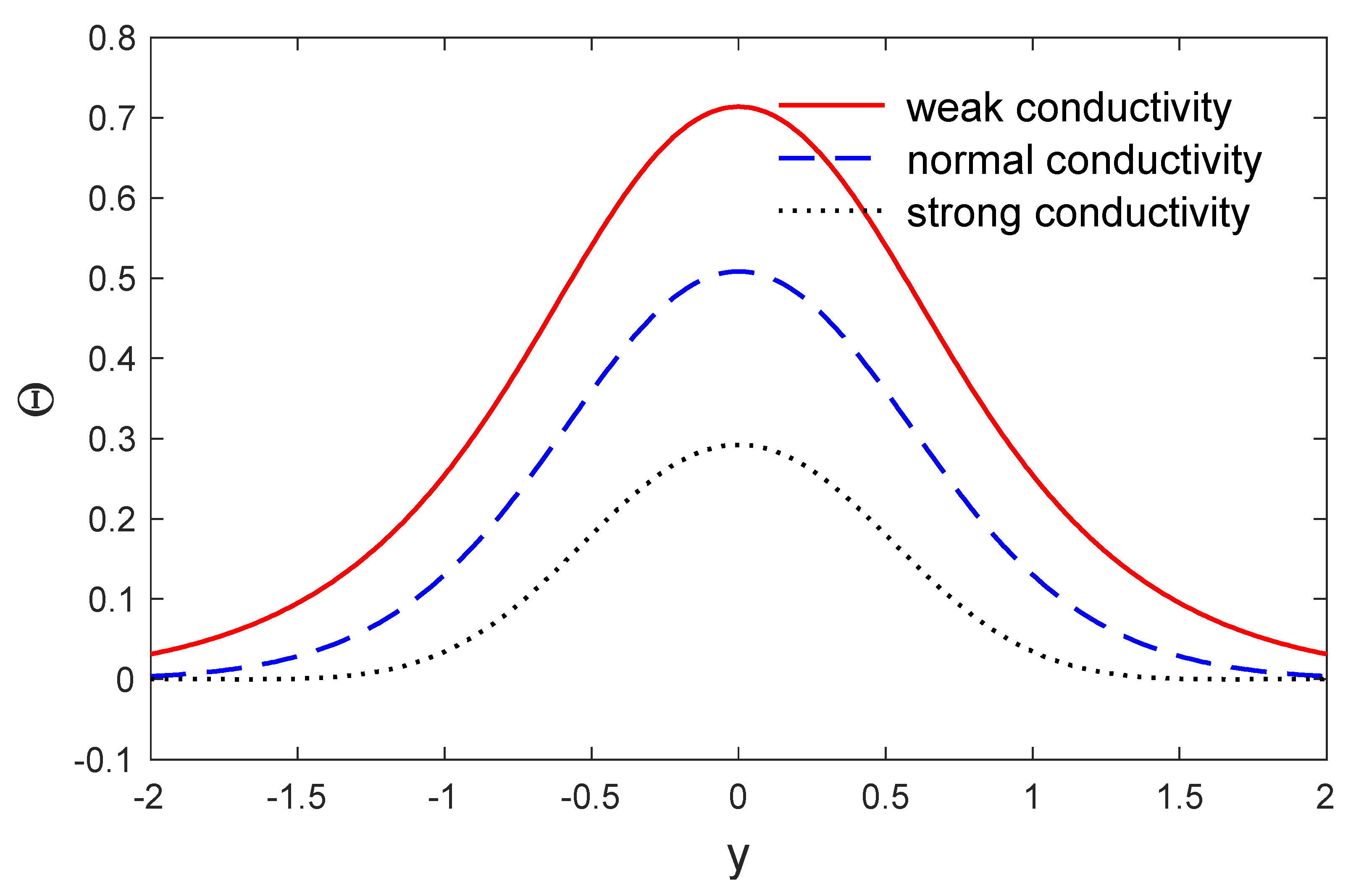
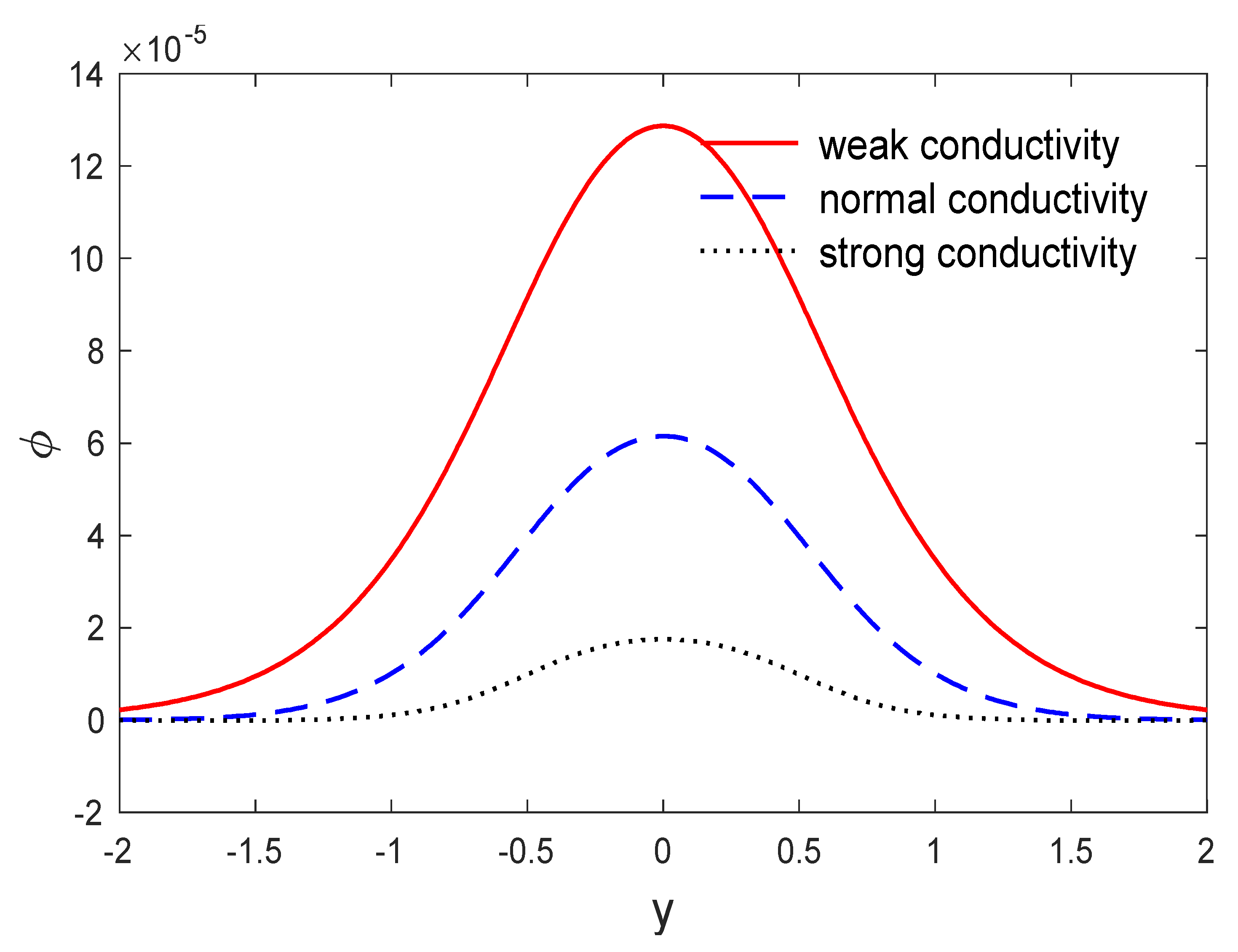
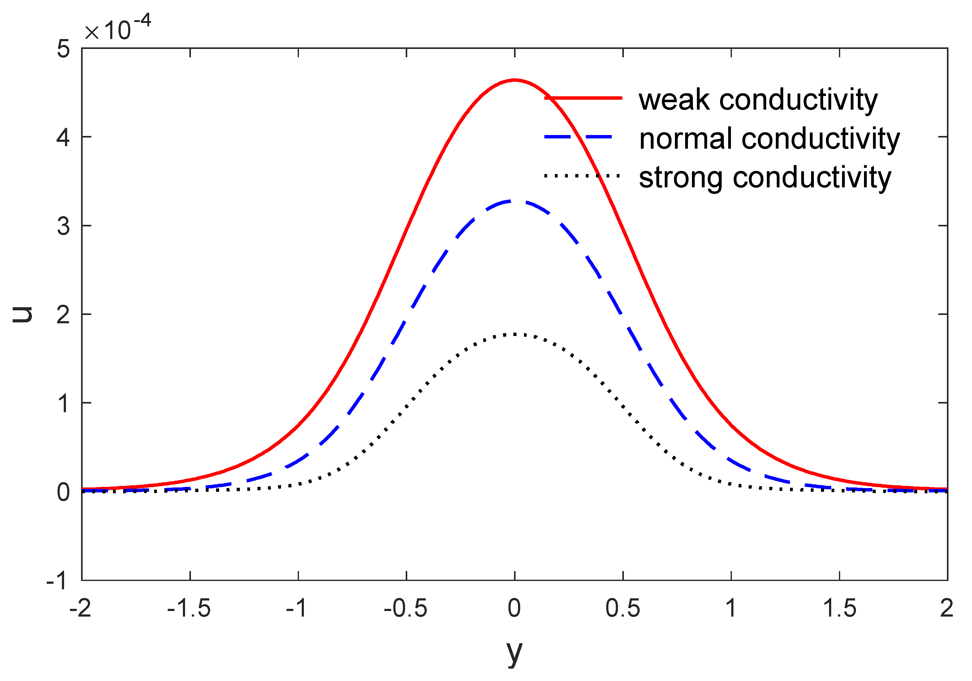
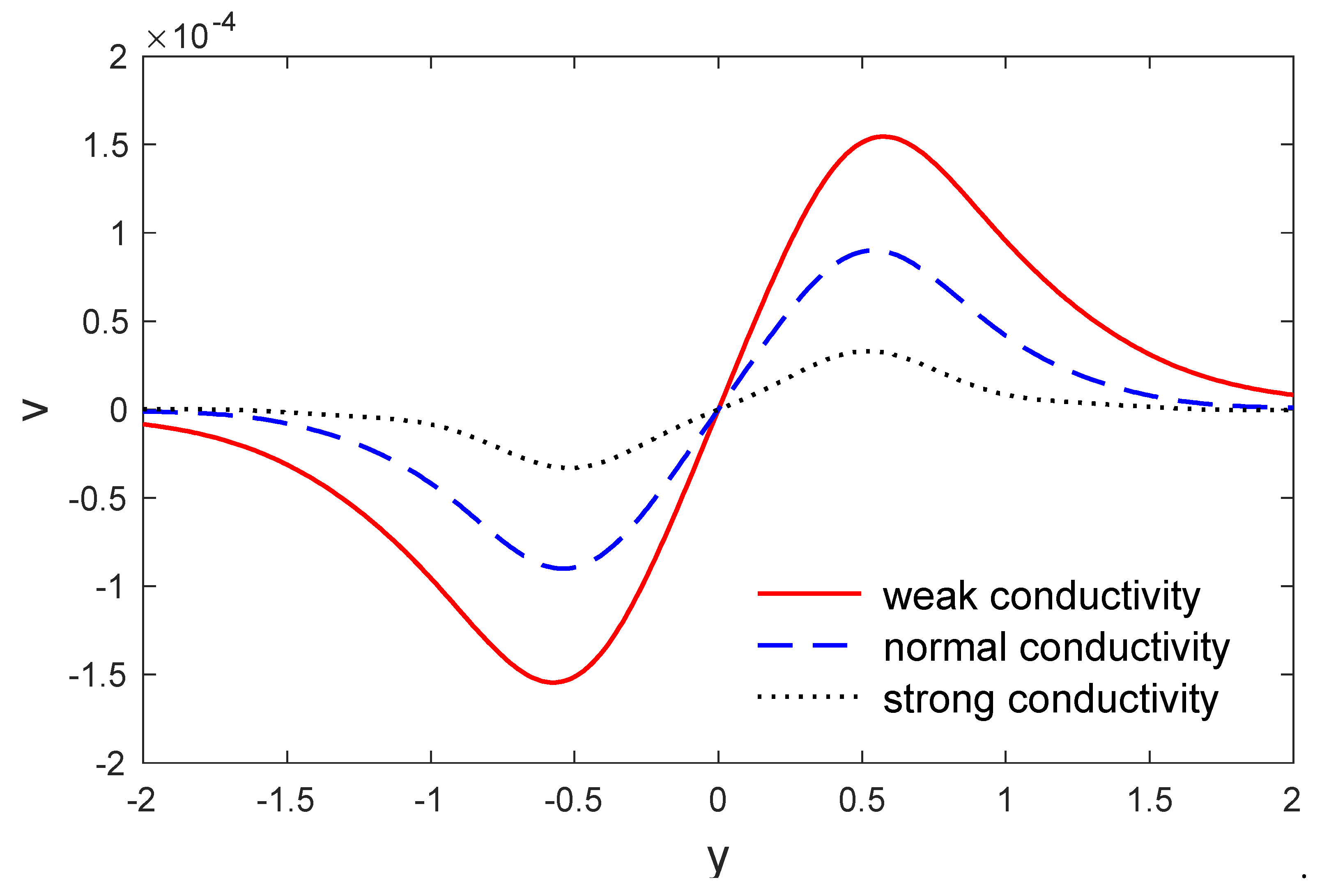
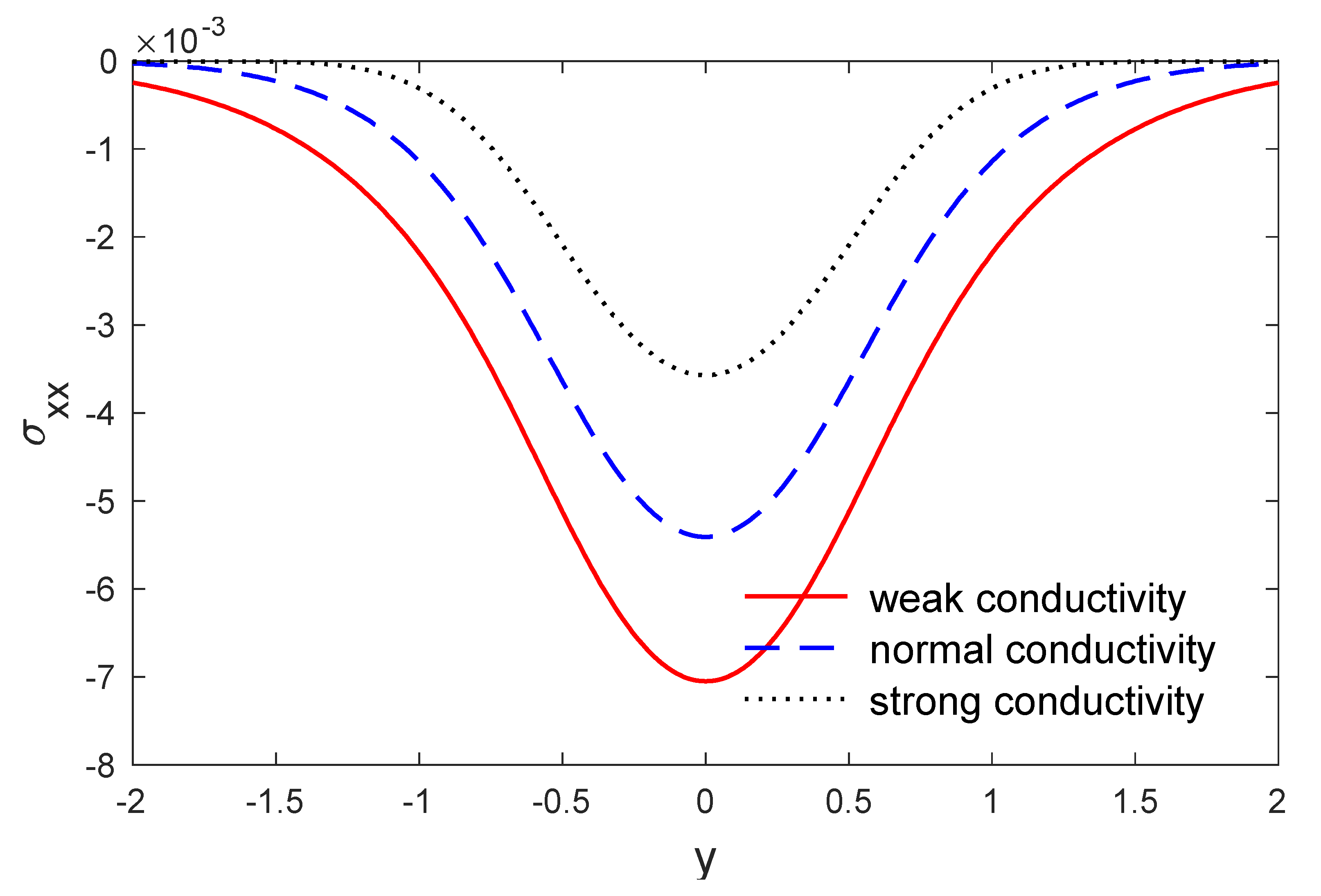
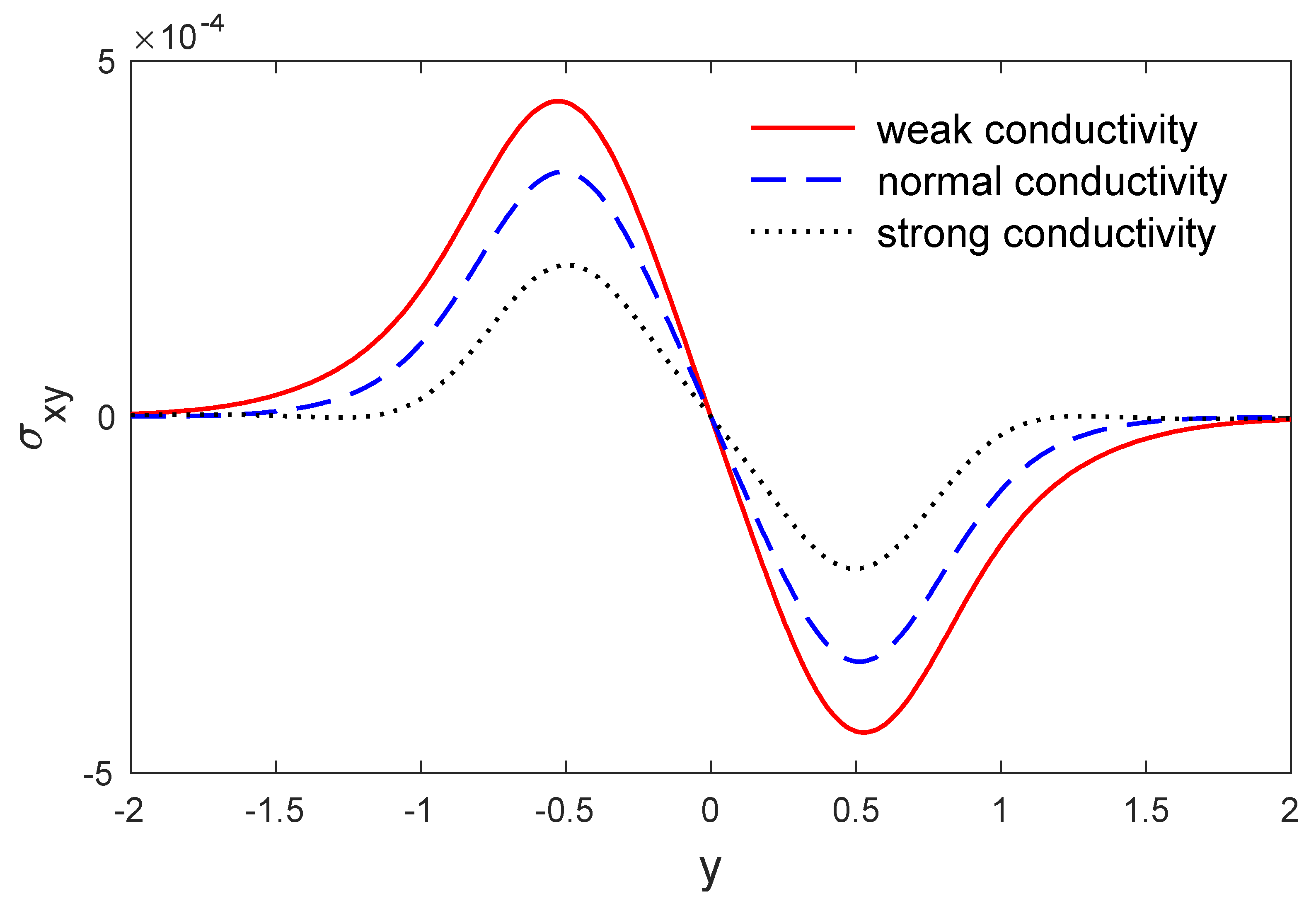
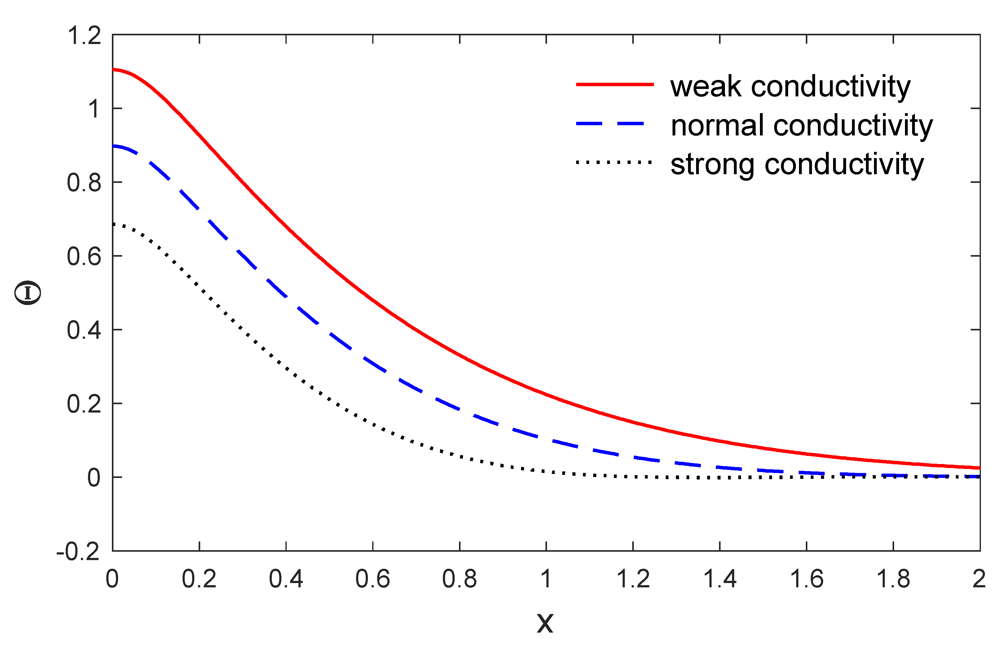
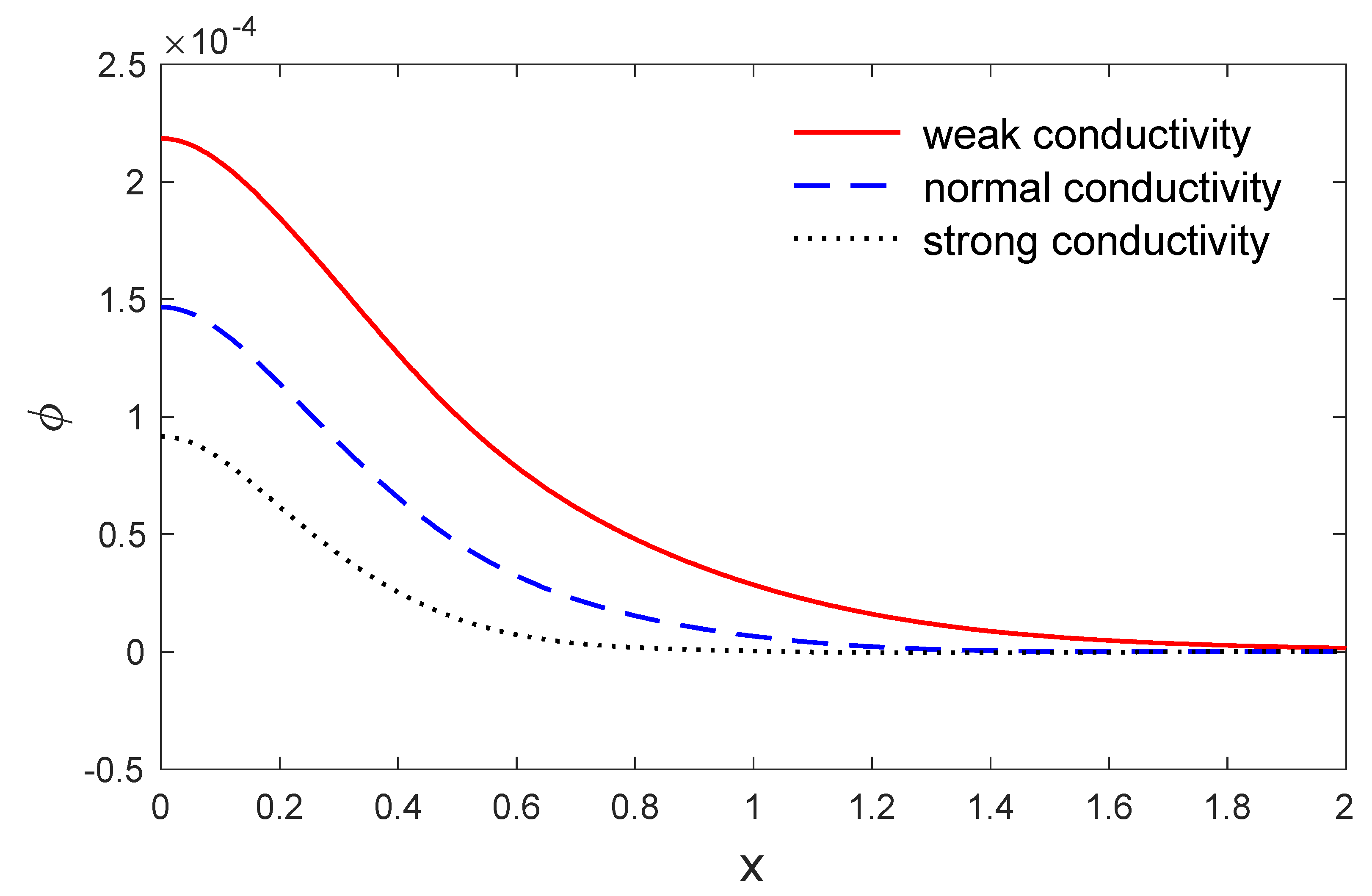
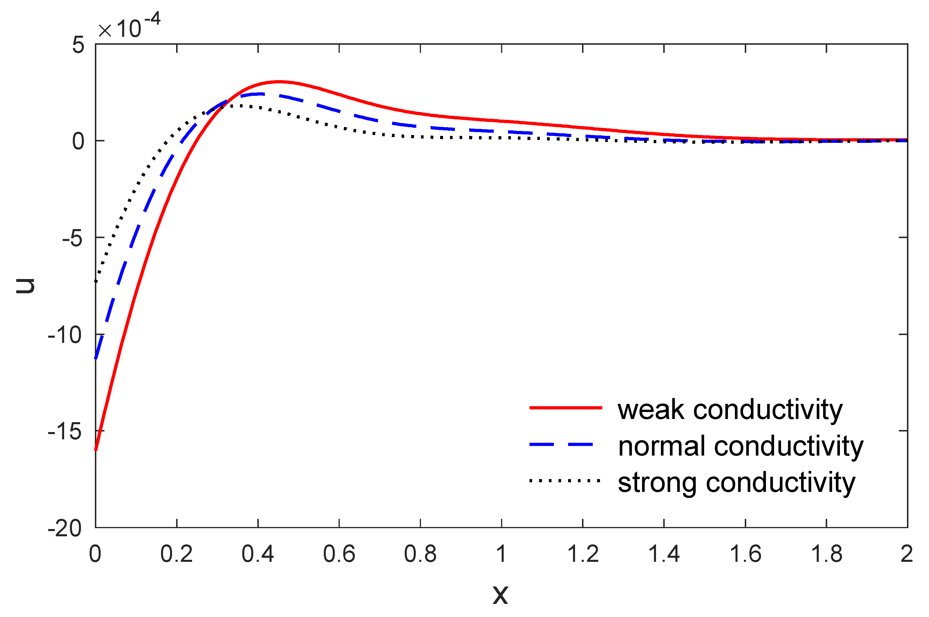
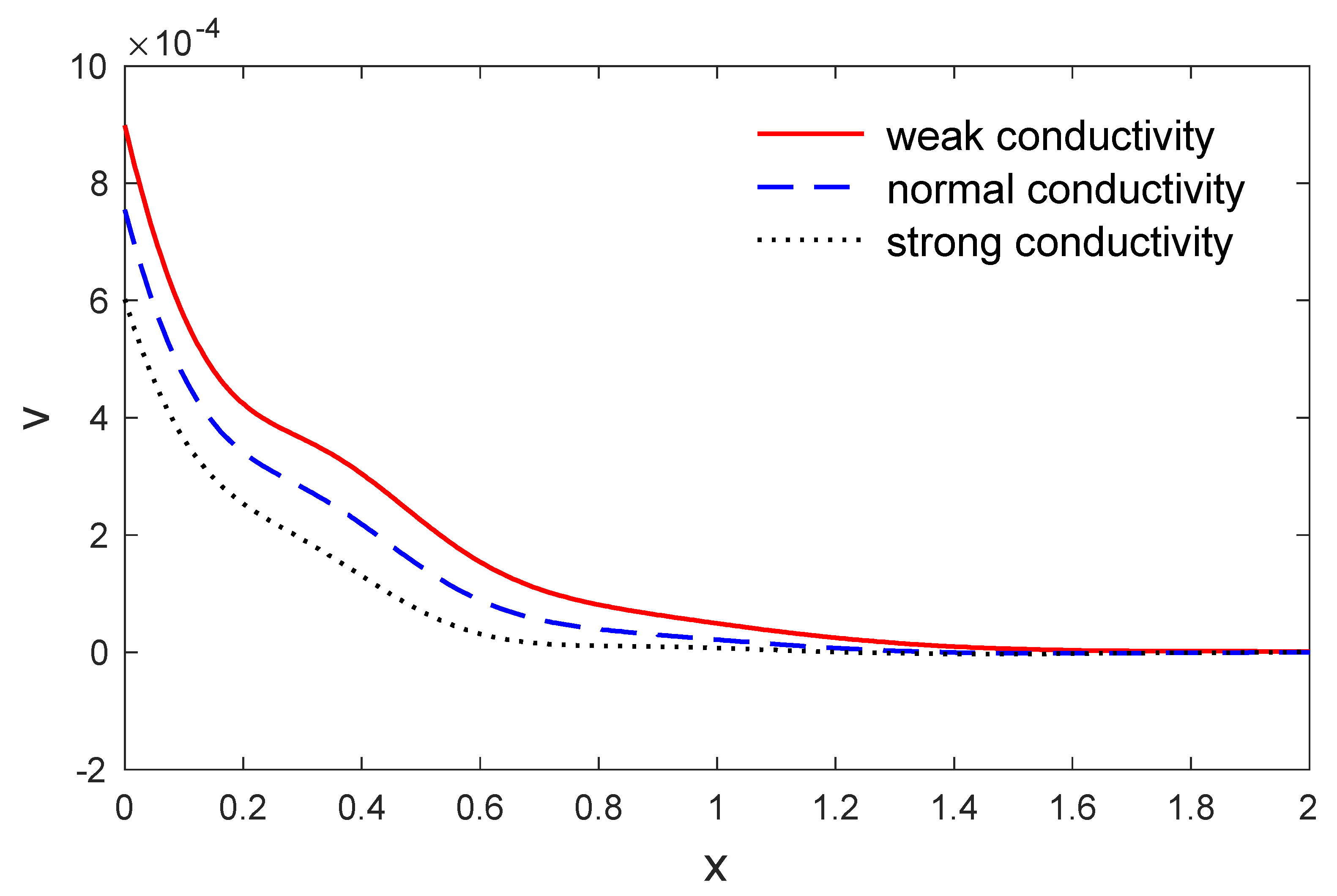
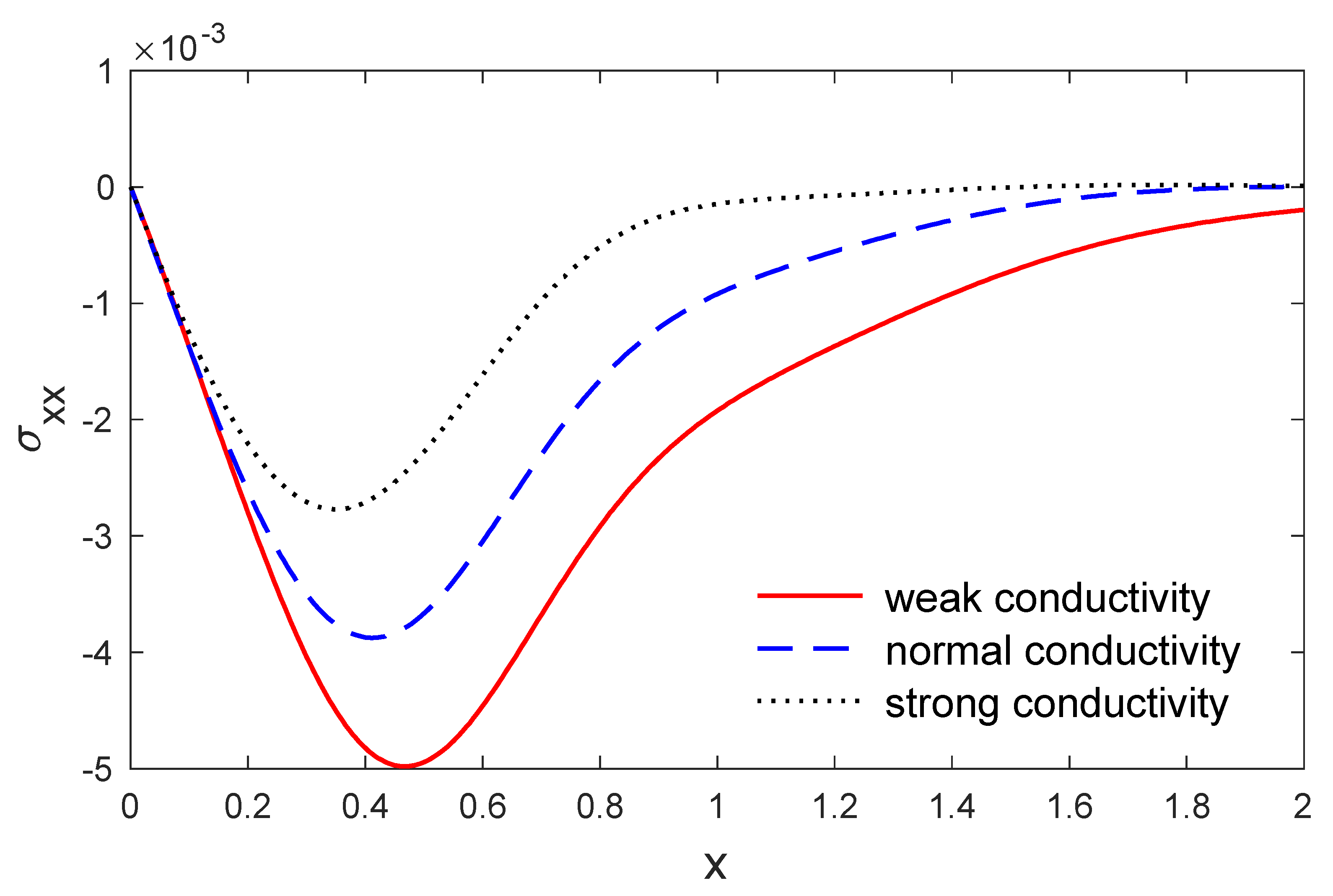
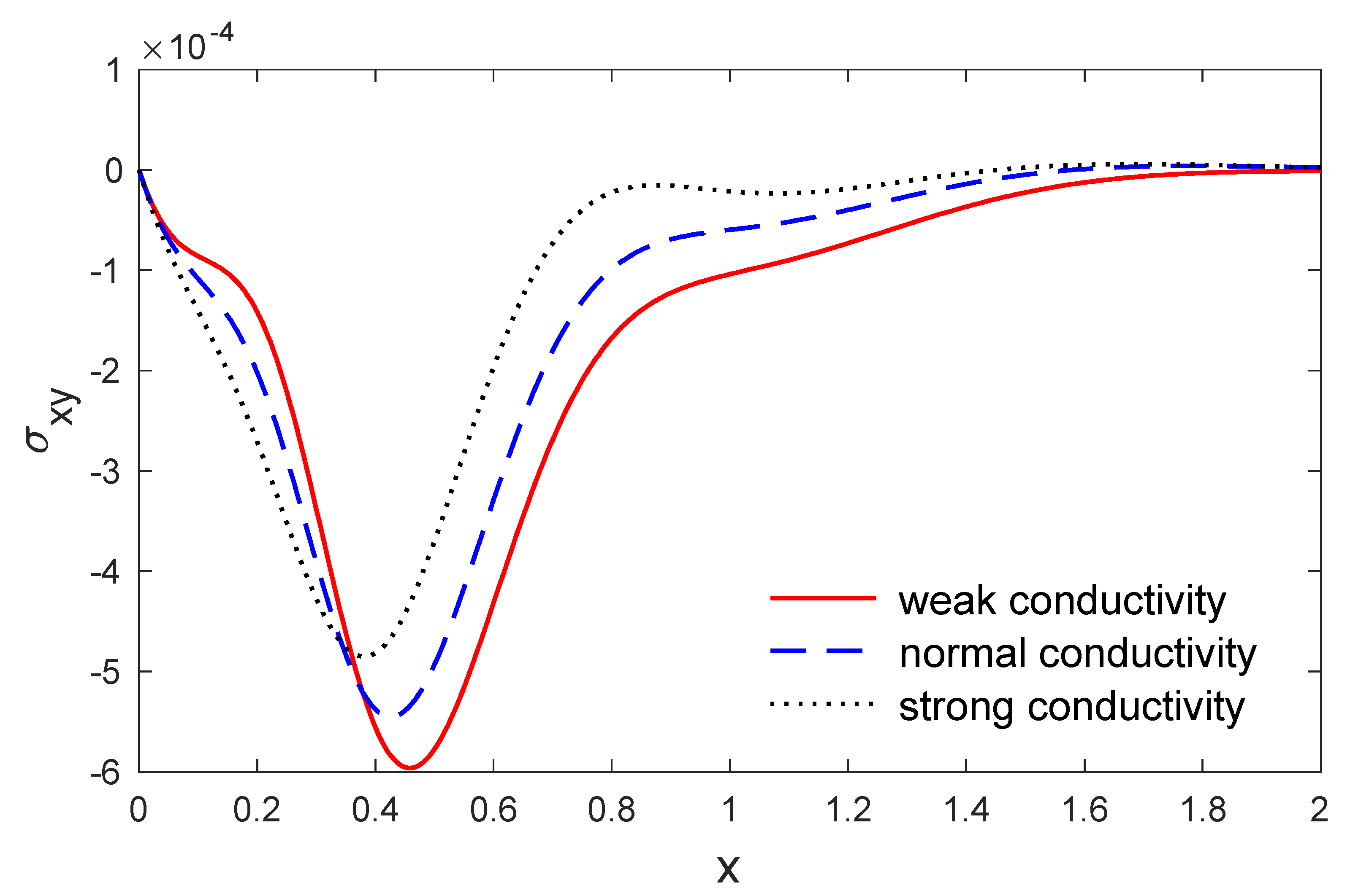
The above list has been applied to investigate the weak, normal and strong thermal conductivities in a two-dimensional porous material by the eigenvalues approach. The voids change in volume fraction field distribution $\phi$, the variation of temperature$\mathsf{\Theta }$, the components of stresses ${\sigma }_{xx}, {\sigma }_{xy}$ and the components of displacement $u, v$ were investigated. The material was considered to be an isotropic and homogeneous two-dimension medium and all the physical quantities were used here as the dimensionless quantities. Figure 2 and Figure 3 depict the variation in temperature $\mathsf{\Theta }$ and the change in the volume fraction field of voids variation $\phi$ versus the distances $y$ when $x=0.5$. It is clear that the variation in the change of the volume fraction field of voids and the variation in temperature have maximum values at the length of the thermal surface $\left(\left(\left|y\right|\le 0.50\right)\right)$, and then begins to decreases completely near the edge $\left(\left(\left|y\right|\le 0.50\right)\right)$, where they decrease and finally reach a zero value. Figure 4 displays the variation in horizontal displacement $u$with respect to the distance $x$. It is clear that it has the ultimate values at the length of the thermal surface $\left(\left|y\right|\le 0.50\right),$and it begins to decrease completely near the edges $\left(y=\pm 0.50\right)$, and after that reduces to zero. Figure 5 displays the variations in vertical displacement $v$ with respect to the distance $y$. It is indicated that it starts the increasing at the beginning and ending of the heating surface $\left(\left|y\right|\le 0.50\right)$, and has a small value at the middle of the heating surface; then it starts the rising and gets close to the ultimate values totally near the edge $\left(y=\pm 0.5\right)$, after that it decreases to close to zero. The components of stress ${\sigma }_{xx}$ and ${\sigma }_{xy}$ along $y$are displayed in Figure 6, Figure 7 and Figure 8. Figure 9 displays the increments of temperature along the distance $x$. It is noticed that it begins from the utmost value according to the applications of boundary conditions and decreases with the increasing $\mathrm{x}$to close to zero. Figure 9 shows the change in the volume fraction field of the voids distribution $\phi$ with respect to the distances $x$. It is observed that the change in the volume fraction field of voids decreases with increases in $x$, until attaining zero. Figure 10 predicts the variation of horizontal displacement $u$ versus $x$. It is clear that it attains the maximum negative values and progressively increases till it attains peak values at a particular location in close proximity to $x=0.0$, and then decreases to close to zero. Figure 11 shows the variation in vertical displacement along x, which has its maximum value on $x=0$ and decreases with an increasing $x$. Figure 12 and Figure 13 predict the stress components variation ${\sigma }_{xx}$ and ${\sigma }_{xy}$ along $x$. It is observed that the magnitudes of stress constantly began from zero, which satisfied the problem boundary conditions.

Finally, Figure 2, Figure 3, Figure 4, Figure 5, Figure 6, Figure 7, Figure 8, Figure 9, Figure 10, Figure 11, Figure 12 and Figure 13 show the variation of all the physical quantities with respect to the distance $y$ and the distance $x$ at $t=0.6$. These figures show the predicted curves through the weak, normal and strong thermal conductivities. As expected, it can be found that the weak, normal and strong thermal conductivity stages have the major impact on the values of all the physical quantities.

5. Conclusions

The results of this work present the fractional-order generalized thermo-elasticity theory as a new improvement and progress in the field of thermo-elasticity. According to this theory, we have to construct a new classification for all the materials according to its fractional parameter, where this parameter becomes a new indicator of its ability to conduct the thermal energy. We discovered that the parameter of fractional-order has significant impacts in all the fields studied, as well as in the outcomes that support the definitions of the classifications of the thermal conductivity of the three types of mediums: weak, normal and strong thermal conductivities. Accordingly, we can consider the generalized thermo-elastic model of fractional-orders as an advancement in the study of elastic porous media. We have to make new classifications of the materials according to the values of the parameter that points to the conductivity of the materials.

References

- Biot, M.A. Thermoelasticity and irreversible thermodynamics. J. Appl. Phys. 1956, 27, 240–253. [Google Scholar] [CrossRef]
- Lord, H.W.; Shulman, Y. A generalized dynamical theory of thermoelasticity. J. Mech. Phys. Solids 1967, 15, 299–309. [Google Scholar] [CrossRef]
- Youssef, H.M. Theory of fractional order generalized thermoelasticity. J. Heat Transf. 2010, 132, 1–7. [Google Scholar] [CrossRef]
- Youssef, H.M.; Al-Lehaibi, E.A. Variational principle of fractional order generalized thermoelasticity. Appl. Math. Lett. 2010, 23, 1183–1187. [Google Scholar] [CrossRef] [Green Version]
- Ezzat, M.A.; El Karamany, A.S. Theory of fractional order in electro-thermoelasticity. Eur. J. Mech. A/Solids 2011, 30, 491–500. [Google Scholar] [CrossRef]
- Sherief, H.H.; El-Sayed, A.M.A.; Abd El-Latief, A.M. Fractional order theory of thermoelasticity. Int. J. Solids Struct. 2010, 47, 269–275. [Google Scholar] [CrossRef]
- Karageorghis, A.; Lesnic, D.; Marin, L. A moving pseudo-boundary MFS for void detection in two-dimensional thermoelasticity. Int. J. Mech. Sci. 2014, 88, 276–288. [Google Scholar] [CrossRef]
- Singh, B. Wave propagation in a generalized thermoelastic material with voids. Appl. Math. Comput. 2007, 189, 698–709. [Google Scholar] [CrossRef]
- Marin, M.; Ellahi, R.; Chirilă, A. On solutions of Saint-Venant’s problem for elastic dipolar bodies with voids. Carpathian J. Math. 2017, 33, 219–232. [Google Scholar]
- Sarkar, N. Wave propagation in an initially stressed elastic half-space solids under time-fractional order two-temperature magneto-thermoelasticity. Eur. Phys. J. Plus 2017, 132, 154. [Google Scholar] [CrossRef]
- Ezzat, M.; El-Karamany, A.; El-Bary, A. Modeling of memory-dependent derivative in generalized thermoelasticity. Eur. Phys. J. Plus 2016, 131, 372. [Google Scholar] [CrossRef]
- Abbas, I.A. Nonlinear transient thermal stress analysis of thick-walled FGM cylinder with temperature-dependent material properties. Meccanica 2014, 49, 1697–1708. [Google Scholar] [CrossRef]
- Abbas, I.A.; Zenkour, A.M. The effect of rotation and initial stress on thermal shock problem for a fiber-reinforced anisotropic half-space using Green-Naghdi theory. J. Comput. Theor. Nanosci. 2014, 11, 331–338. [Google Scholar] [CrossRef]
- Abbas, I.A.; Marin, M. Analytical solution of thermoelastic interaction in a half-space by pulsed laser heating. Phys. E Low-Dimens. Syst. Nanostructures 2017, 87, 254–260. [Google Scholar] [CrossRef]
- Mohamed, R.; Abbas, I.A.; Abo-Dahab, S. Finite element analysis of hydromagnetic flow and heat transfer of a heat generation fluid over a surface embedded in a non-Darcian porous medium in the presence of chemical reaction. Commun. Nonlinear Sci. Numer. Simul. 2009, 14, 1385–1395. [Google Scholar] [CrossRef]
- Abbas, I.A.; El-Amin, M.; Salama, A. Effect of thermal dispersion on free convection in a fluid saturated porous medium. Int. J. Heat Fluid Flow 2009, 30, 229–236. [Google Scholar] [CrossRef]
- Abbas, I.A. Generalized magneto-thermoelasticity in a nonhomogeneous isotropic hollow cylinder using the finite element method. Arch. Appl. Mech. 2009, 79, 41–50. [Google Scholar] [CrossRef]
- Abbas, I.A. Finite element analysis of the thermoelastic interactions in an unbounded body with a cavity. Forsch. Im Ing. 2007, 71, 215–222. [Google Scholar] [CrossRef]
- Hobiny, A.D.; Abbas, I.A. Fractional order photo-thermo-elastic waves in a two-dimensional semiconductor plate. Eur. Phys. J. Plus 2018, 133, 232. [Google Scholar] [CrossRef]
- Sheikholeslami, M.; Ellahi, R.; Shafee, A.; Li, Z. Numerical investigation for second law analysis of ferrofluid inside a porous semi annulus: An application of entropy generation and exergy loss. Int. J. Numer. Methods Heat Fluid Flow 2019, 29, 1079–1102. [Google Scholar] [CrossRef]
- Ellahi, R.; Sait, S.M.; Shehzad, N.; Ayaz, Z. A hybrid investigation on numerical and analytical solutions of electro-magnetohydrodynamics flow of nanofluid through porous media with entropy generation. Int. J. Numer. Methods Heat Fluid Flow 2019, 30, 834–854. [Google Scholar] [CrossRef]
- Sur, A.; Kanoria, M. Fractional order generalized thermoelastic functionally graded solid with variable material properties. J. Solid Mech. 2014, 6, 54–69. [Google Scholar]
- Qi, H.; Guo, X. Transient fractional heat conduction with generalized Cattaneo model. Int. J. Heat Mass Transf. 2014, 76, 535–539. [Google Scholar] [CrossRef]
- Deswal, S.; Kalkal, K.K. Plane waves in a fractional order micropolar magneto-thermoelastic half-space. Wave Motion 2014, 51, 100–113. [Google Scholar] [CrossRef]
- Youssef, H.M. State-space approach to fractional order two-temperature generalized thermoelastic medium subjected to moving heat source. Mech. Adv. Mater. Struct. 2013, 20, 47–60. [Google Scholar] [CrossRef]
- Othman, M.; Sarkar, N.; Atwa, S.Y. Effect of fractional parameter on plane waves of generalized magneto–thermoelastic diffusion with reference temperature-dependent elastic medium. Comput. Math. Appl. 2013, 65, 1103–1118. [Google Scholar] [CrossRef]
- Youssef, H.M. Two-dimensional thermal shock problem of fractional order generalized thermoelasticity. Acta Mech. 2012, 223, 1219–1231. [Google Scholar] [CrossRef]
- Sur, A.; Kanoria, M. Fractional order two-temperature thermoelasticity with finite wave speed. Acta Mech. 2012, 223, 2685–2701. [Google Scholar] [CrossRef]
- Kothari, S.; Mukhopadhyay, S. A problem on elastic half space under fractional order theory of thermoelasticity. J. Therm. Stresses 2011, 34, 724–739. [Google Scholar] [CrossRef]
- Youssef, H.M.; Al-Lehaibi, E.A. Fractional order generalized thermoelastic half-space subjected to ramp-type heating. Mech. Res. Commun. 2010, 37, 448–452. [Google Scholar] [CrossRef]
- Alzahrani, F.S.; Abbas, I.A. Photo-thermal interactions in a semiconducting media with a spherical cavity under hyperbolic two-temperature model. Mathematics 2020, 8, 585. [Google Scholar] [CrossRef] [Green Version]
- Das, N.C.; Lahiri, A.; Giri, R.R. Eigenvalue approach to generalized thermoelasticity. Indian J. Pure Appl. Math. 1997, 28, 1573–1594. [Google Scholar]
- Abbas, I.A. The effects of relaxation times and a moving heat source on a two-temperature generalized thermoelastic thin slim strip. Can. J. Phys. 2015, 93, 585–590. [Google Scholar] [CrossRef]
- Abbas, I.A.; Alzahrani, F.S.; Elaiw, A. A DPL model of photothermal interaction in a semiconductor material. Waves Random Complex Media 2019, 29, 328–343. [Google Scholar] [CrossRef]
- Stehfest, H. Algorithm 368: Numerical inversion of Laplace transforms [D5]. Commun. ACM 1970, 13, 47–49. [Google Scholar] [CrossRef]
- Othman, M.I.; Marin, M. Effect of thermal loading due to laser pulse on thermoelastic porous medium under GN theory. Results Phys. 2017, 7, 3863–3872. [Google Scholar] [CrossRef]
Figure 1.
Geometry of the problem.
Figure 2.
The variations in temperature along when x , for weak, normal and strong conductivities.
Figure 3.
The changes in the volume fraction field of the voids distribution φ along y when x = 0.5, for weak, normal and strong conductivities.
Figure 4.
The variation in horizontal displacement u along y when x = 0.5, for weak, normal and strong conductivities.
Figure 5.
The variation in vertical displacement along when x , for weak, normal and strong conductivities.
Figure 6.
The variation in stress along when x , for weak, normal and strong conductivities.
Figure 7.
Figure 8.
The variation in temperature along when y , for weak, normal and strong conductivities.
Figure 9.
The changes in the volume fraction field of the voids distribution along when y , for weak, normal and strong conductivities.
Figure 10.
The variation in horizontal displacement along when y , for weak, normal and strong conductivities.
Figure 11.
The variation in vertical displacement along when y , for weak, normal and strong conductivities.
Figure 12.
The variation in stress along when y , for weak, normal and strong conductivities.
Figure 13.
© 2020 by the authors. Licensee MDPI, Basel, Switzerland. This article is an open access article distributed under the terms and conditions of the Creative Commons Attribution (CC BY) license (http://creativecommons.org/licenses/by/4.0/).
Share and Cite
MDPI and ACS Style
Alzahrani, F.; Hobiny, A.; Abbas, I.; Marin, M. An Eigenvalues Approach for a Two-Dimensional Porous Medium Based Upon Weak, Normal and Strong Thermal Conductivities. Symmetry 2020, 12, 848. https://doi.org/10.3390/sym12050848
AMA Style
Alzahrani F, Hobiny A, Abbas I, Marin M. An Eigenvalues Approach for a Two-Dimensional Porous Medium Based Upon Weak, Normal and Strong Thermal Conductivities. Symmetry. 2020; 12(5):848. https://doi.org/10.3390/sym12050848
Chicago/Turabian StyleAlzahrani, Faris, Aatef Hobiny, Ibrahim Abbas, and Marin Marin. 2020. "An Eigenvalues Approach for a Two-Dimensional Porous Medium Based Upon Weak, Normal and Strong Thermal Conductivities" Symmetry 12, no. 5: 848. https://doi.org/10.3390/sym12050848
Note that from the first issue of 2016, this journal uses article numbers instead of page numbers. See further details here.