A Study on Domination in Vague Incidence Graph and Its Application in Medical Sciences


Institute of Computing Science and Technology, Guangzhou University, Guangzhou 510006, China
*
Author to whom correspondence should be addressed.
Symmetry 2020, 12(11), 1885; https://doi.org/10.3390/sym12111885
Submission received: 26 October 2020
/
Revised: 10 November 2020
/
Accepted: 11 November 2020
/
Published: 16 November 2020
(This article belongs to the Section Mathematics)
Abstract
:Fuzzy graphs (FGs), broadly known as fuzzy incidence graphs (FIGs), have been acknowledged as being an applicable and well-organized tool to epitomize and solve many multifarious real-world problems in which vague data and information are essential. Owing to unpredictable and unspecified information being an integral component in real-life problems that are often uncertain, it is highly challenging for an expert to illustrate those problems through a fuzzy graph. Therefore, resolving the uncertainty accompanying the unpredictable and unspecified information of any real-world problem can be done by applying a vague incidence graph (VIG), based on which the FGs may not engender satisfactory results. Similarly, VIGs are outstandingly practical tools for analyzing different computer science domains such as networking, clustering, and also other issues such as medical sciences, and traffic planning. Dominating sets (DSs) enjoy practical interest in several areas. In wireless networking, DSs are being used to find efficient routes with ad-hoc mobile networks. They have also been employed in document summarization, and in secure systems designs for electrical grids; consequently, in this paper, we extend the concept of the FIG to the VIG, and show some of its important properties. In particular, we discuss the well-known problems of vague incidence dominating set, valid degree, isolated vertex, vague incidence irredundant set and their cardinalities related to the dominating, etc. Finally, a DS application for VIG to properly manage the COVID-19 testing facility is introduced.
1. Introduction
The graph concept stands as one of the most dominant and widely employed tools for the multiple real-world problem representation, modeling, and analyses. To represent the objects and the relations between them, the graph vertices and edges are applied, respectively. FG-models are beneficial mathematical tools for addressing the combinatorial problems in various fields involving research, optimization, algebra, computing, environmental science, and topology. Thanks to the natural existence of vagueness and ambiguity, fuzzy graphical models are strikingly better than graphical models. Originally, fuzzy set theory was required to contend with many multidimensional issues, which are replete with incomplete information. In 1965 [1], fuzzy set theory was first proposed by Zadeh. Fuzzy set theory is a highly influential mathematical tool for solving approximate reasoning related problems. By presenting the VS notion through changing the value of an element in a set with a sub-interval of , Gau and Buehrer [2] introduced and structured the vague set theory. The VSs describe more possibilities than fuzzy sets. A VS is more effective for the existence of the false membership degree. An immediate result of a rise of popularity of fuzzy sets theory has been the fuzzification of graph theory which has been initiated by Rosenfeld [3] who has introduced the concept of a fuzzy graph. The incidence graphs can generally be represented as a triple , where V is a finite set of vertices and E is a finite set of edges, and is an incidence function which indicates for each edge its end vertices and whether the edge is directed (1) or not (0). If an edge e is directed, then the first element and the second element of denote the origin vertex and the destination vertex, respectively.
The origins of the concept of an incidence graph is often attributed to Brualdi and Massey [4] who have been dealing with the incidence and incidence chromatic number. The fuzzification of the incidence graphs has been proposed by Dinesh [5,6], and among later contributions a special place belongs to the works by Mordeson and his collaborators, notably Mathew, Mordeson and Malik [7] or Mordeson and Mathew [8,9,10,11]. Ramakrishna [12] recommended the VG notion and evaluated some of its features. Akram et al. [13,14,15] presented new definitions of FGs. Borzooei and Rashmanlou [16,17,18,19] investigated different concepts on VG. Shao et al. [20,21,22,23] presented some results in VGs and intuitionistic fuzzy graphs. Samanta et al. [24,25,26,27] defined fuzzy competition graphs and some properties of bipolar fuzzy graphs. Rashmanlou et al. [28,29,30,31] introduced new concepts in VGs.
Domination in graphs has many applications to several fields. Domination arises in facility location problems, where the number of facilities (e.g., hospital, fire stations) is fixed and one attempts to minimize the distance that a person needs to travel to the closest facility. Concepts from DS also appear in problems involving finding sets of representative in monitoring communication or electrical networks. The concept of a domination in an FG was introduced by Somasundaram [32]. Parvathi and Thamizhendhi [33] described the concept of a domination number in an intuitionistic fuzzy graph. Gani et al. [34] gave some properties of a fuzzy-DS, and a fuzzy irredundant set. Many researchers, notably Talebi and Rashmanlou [35], studied new applications of the concept of domination in VGs. The vague incidence model is more compliant and functioning than fuzzy and intuitionistic incidence fuzzy models. In several applications, such as urban traffic planning, telecommunication message routing, very large-scale integration chip optimal pipelining, etc., VIGs serve as the observed real-world systems mathematical models. Therefore, in this research, we extend the concept of the FIG to the VIG and discuss the well-known problems of vague incidence dominating set (VIDS), valid degree, vague incidence irredundant set (VIIS), and their cardinalities related to the domination, etc.
Many people today suffer from COVID-19 virus and in some cases die. Unfortunately, the lack of necessary facilities in hospitals and clinics has multiplied the possibility of the virus outbreak. Hence, an application of DS for VIG to properly manage the COVID-19 testing facility is introduced.
2. Preliminaries
In this section, to set the stage for our analysis, and to facilitate the following of our discussion, we show a brief overview of some of the basic definitions. A graph is a pair of that holds . The elements of and are the nodes and edges of the graph G, respectively. An FG is of the form which is a pair of mapping and as is defined as , , and is a symmetric fuzzy relation on and ∧ denotes the minimum.
Definition 1.
[4] Let be a graph. Then, is called an incidence graph, so that . If , and , then is an incidence graph even though . The pair is called an incidence pair or simply a pair. If , then or are called adjacent edges.
Definition 2.
[6] Let be an incidence graph and σ be a fuzzy subset of V and μ, a fuzzy subset of E. Let ψ be a fuzzy subset of I. If , for all and , then, ψ is called a fuzzy incidence of graph and is called a FIG of .
Definition 3.
[2] A VS A is a pair on set V where and are taken as real valued functions which can be defined on , so that , for all m belongs V. The interval is known as the vague value of m in A.
Definition 4.
[12] A pair is said to be a VG on a crisp graph , where is a VS on V and is a VS on such that and , for each edge .
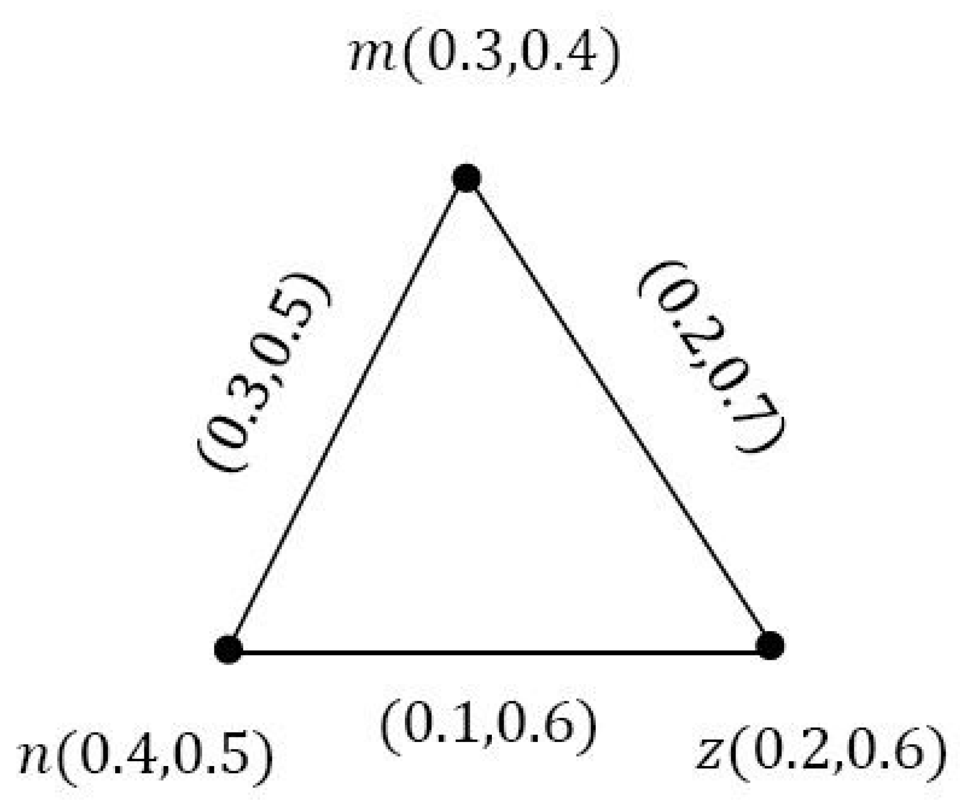
Example 1.
Consider a VG G such that and , as shown in Figure 1.
By routine computations, it is easy to show that G is a VG.
Definition 5.
[21] The strength of a vague edge of a VG is given as:
Definition 6.
[21] A vague edge of a VG is said to be vague strong edge whenever or , otherwise is vague weak edge.
All the basic notations are shown in Table 1.
3. Vague Incidence Graph
A natural follow-up to the concept of a VG, outlined in the previous section, is the concept of a VIG which will now be presented with its main properties. Also, we will discuss a very important concept of domination on VIG.
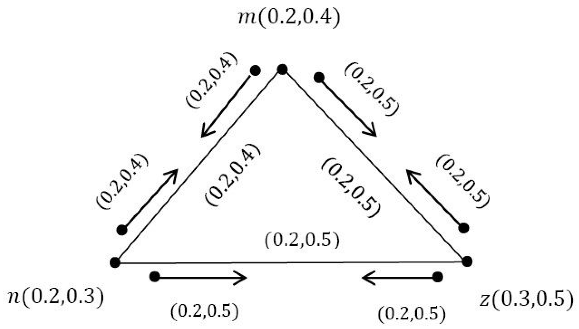
Definition 7.
is called a VIG of underlying crisp incidence graph , if
such that
and , , .
Example 2.
Definition 8.
The support of a VIG is so that:
Definition 9.
If is a VIG, then, is a VI-subgraph of ζ whenever , , and .
Definition 10.
If is a VIG, then, a vague incidence edge of ζ is called a vague incidence valid edge if
and
and otherwise it is called a vague incidence invalid edge.
Definition 11.
If ζ is a VIG, then, its cardinality is defined as:
and also, we have:
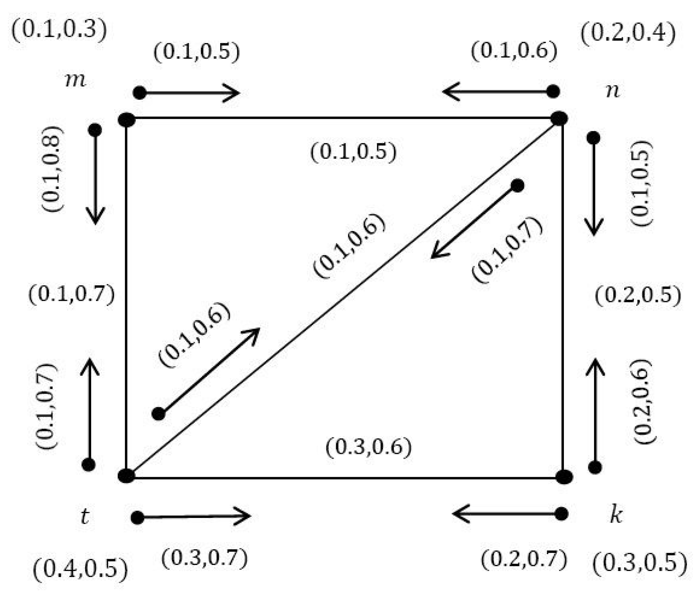
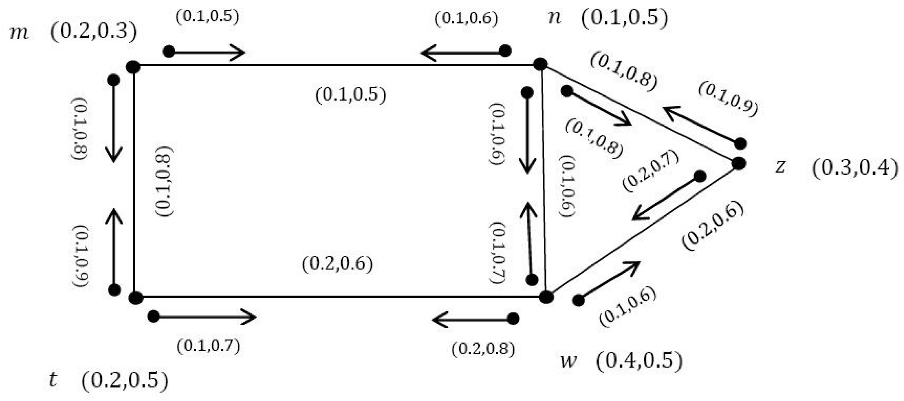
Example 3.
Consider a VIG, ζ as shown in Figure 4.
Here, the edges of , , and are the vague incidence valid edges.
Example 4.
In Figure 4, it is obvious that and are vague incidence valid edges and we have:
Definition 12.
The VIG is said to be complete if:
and .
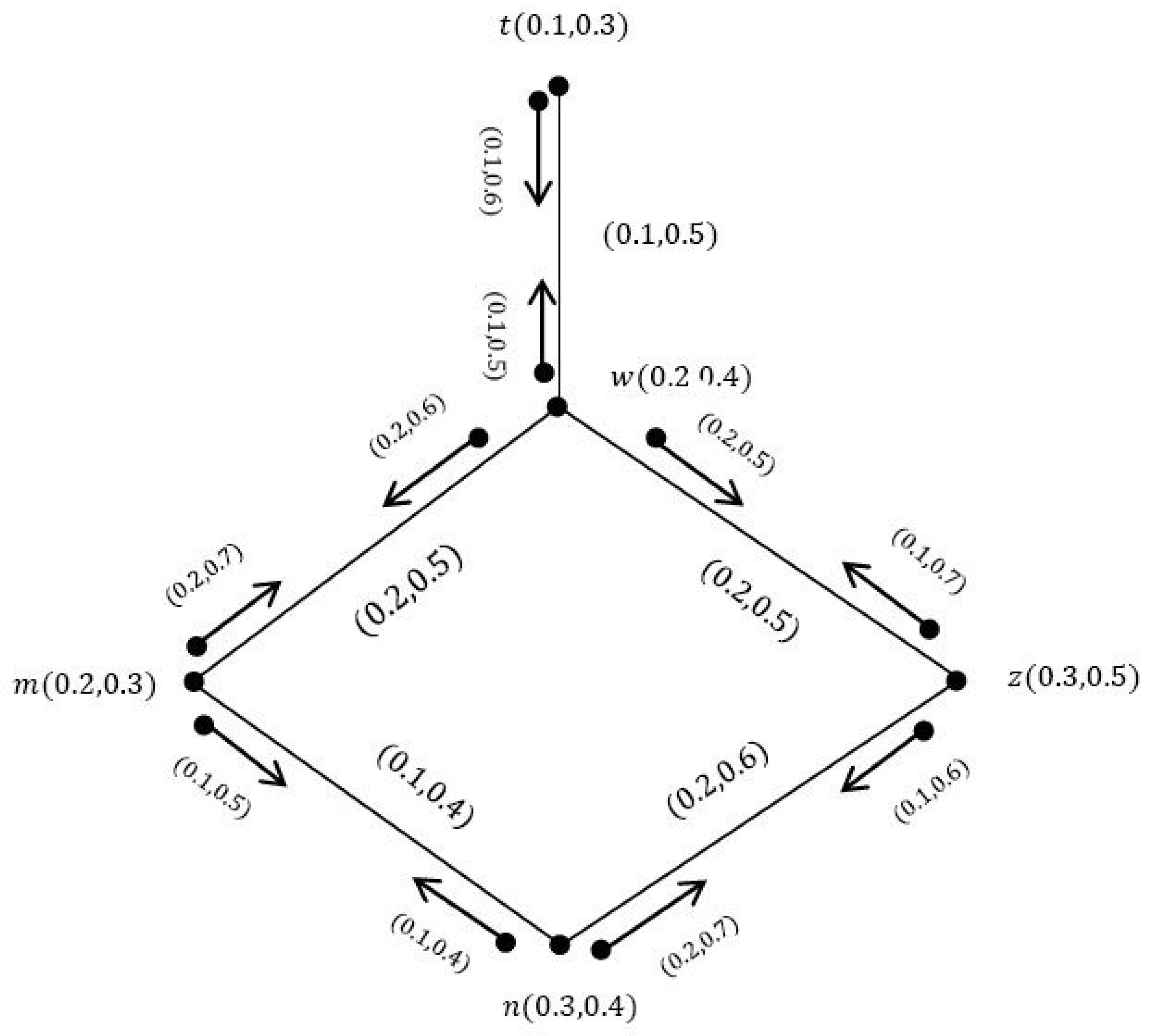
Example 5.
Consider a VIG, ζ as shown in Figure 5.
It is easy to see that ζ is a complete VIG.
Definition 13.
If is a VIG, then, a vague incidence valid neighbor of m, is defined as:
Moreover, is called a closed vague incidence valid neighborhood of m.
For non-empty set of D, we have
Definition 14.
The vague incidence valid neighborhood degree of vertex m is defined as:
and the minimum and maximum cardinality vague incidence valid neighborhood degrees of ζ are denoted by and , respectively.
Example 6.
In Figure 5, we have:
Definition 15.
If is a VIG, then, the vertex cardinality of is defined as
Definition 16.
If is a VIG of , then, we say that incidentally dominates in ζ whenever .
Definition 17.
A non-empty set of vertices is called a VIDS in a VIG ζ whenever there exists so that m incidentally dominates n, i.e., , for all .
Definition 18.
The minimum cardinality of VIDSs in a VIG ζ is called a vague incidence domination number of ζ and it is denoted by ; clearly .
A set with the minimum vague cardinality equal , is called an -set or a minimal VIDS.
Example 8.
Let be a VIG as shown in Figure 6. The edges , , , and are vague incidence valid edges. In Figure 6, the sets , , , and are VIDSs. By calculating the cardinalities, we have:
Hence, and is a -set.
Theorem 1.
In any VIG, , there holds
Proof.
Let x be a vertex in a VIG, . Assume that . Then, is a VIDS of , so that
☐
Definition 19.
A VIDS D of a VIG ζ is called a minimal VIDS whenever any proper subset of D is not a VIDS of ζ.
The upper vague incidence domination number equals to the maximum vague cardinality of the minimal VIDSs in . Clearly, is minimum vague cardinality of the minimal VIDS in .
Example 9.
In Example 3, the sets , , , and are the minimal VIDSs. Therefore, and .
Definition 20.
The valid degree of a vertex m in a VIG is defined to be the sum of the true membership and false membership degree of the vague incidence valid edges incident at vertex m, and it is denoted by . The minimum valid degree cardinality and the maximum valid degree cardinality of ζ are denoted by and , respectively.
Example 10.
In Figure 4, we have:
Theorem 2.
If is a VIG of order p, then
Proof.
If D is a minimal VIDS of a VIG , then
Hence, . ☐
Definition 21.
In a VIG , a vertex is called an isolated vertex if , i.e., for any where , is not a vague incidence valid edge.
Example 11.
In Figure 4 we see that n is an isolated vertex because .
Theorem 3.
If be a VIG without isolated vertices and D is the minimal VIDS in ζ, then is a VIDS.
Proof.
Assume D is any minimal VIDS of and vertex incidentally is not dominated by any vertex in . Since has no isolated vertex, m must incidentally be dominated by at least one vertex in , then is a VIDS, which is a contradiction with the minimality of D. Therefore, any vertex in D incidentally is dominated by at least one vertex in and so is a VIDS. ☐
Corollary 1.
For a VIG without isolated vertex, we have .
Proof.
If D is a minimal VIDS of , then, is too. Therefore, . Thus, at least one of the sets D or , has the cardinality equal or less. ☐
Definition 22.
Let be a VIG, and . A vertex n is said a vague incidence valid private neighborhood of m into S, if ; we also denote the vague incidence valid private neighborhood of m into S by . Obviously,
Clearly, if , then, m is isolated in .
Example 12.
Consider the VIG as shown in Figure 7. All edges are clearly vague incidence valid. Let . Then, we have:
Definition 23.
Let be a VIG and . Then, S is said to be a vague incidence irredundant set (VIIS) if, for any , there holds .
Definition 24.
The VIIS S is called a maximal VIIS if, for any , the set is not a VIIS.
Definition 25.
The minimum cardinality among all maximal-VIISs, is called a vague incidence irredundance number ant it is denoted by .
The maximum cardinality among all maximal-VIISs, is called an upper vague incidence irredundance number ant it is denoted by . It is clear that .
Example 13.
In Figure 7, it is easy to see that is the only maximal VIIS and we have .
Theorem 4.
For the VIG , there holds
Proof.
Let S be VIIS in and . Assume that m is a valid neighborhood to k vertices in S. Since the degree of m is at least , m must be valid neighborhood to at least vertices in where is the cardinality of k valid neighborhood vertices m in S. If , then, , i.e., , as required. If , then, each valid neighbor of m in S must have a valid private neighborhood in and these k vertices must be distinct. Hence,
that is, or . ☐
Theorem 5.
A VIDS in a VIG is a minimum VIDS if and only if it is VIIS.
Proof.
Let S be a minimal VIDS in . Then, for any vertex , there exists a vertex which is not dominated by . Therefore, for any , there holds . Thus, any vertex , has at least one incidence valid private neighborhood. Hence, S is both a VDS and a VIDS. Suppose that set S is not a minimal VIDS. Then, there exists an such that is a VDS. Since S is a VIIS, then we obtain that . Let . Then, w is not a valid neighborhood for any vertex in , i.e., is not a VDS which is a contradiction. ☐
Theorem 6.
Each minimal VIDS in a VIG is a maximal VIIS.
Proof.
Due to Theorem 5, any minimal VIDS is a VIIS. Therefore, we just need to show that S is a minimal VIIS. If S is not a minimal VIDS, then, there exists a vertex such that is a VIIS. This means, , so there exists at least one vertex n that is a valid private neighborhood of m into . Hence, no vertex in S is a neighborhood to n. This is a contradiction to S being a DS. ☐
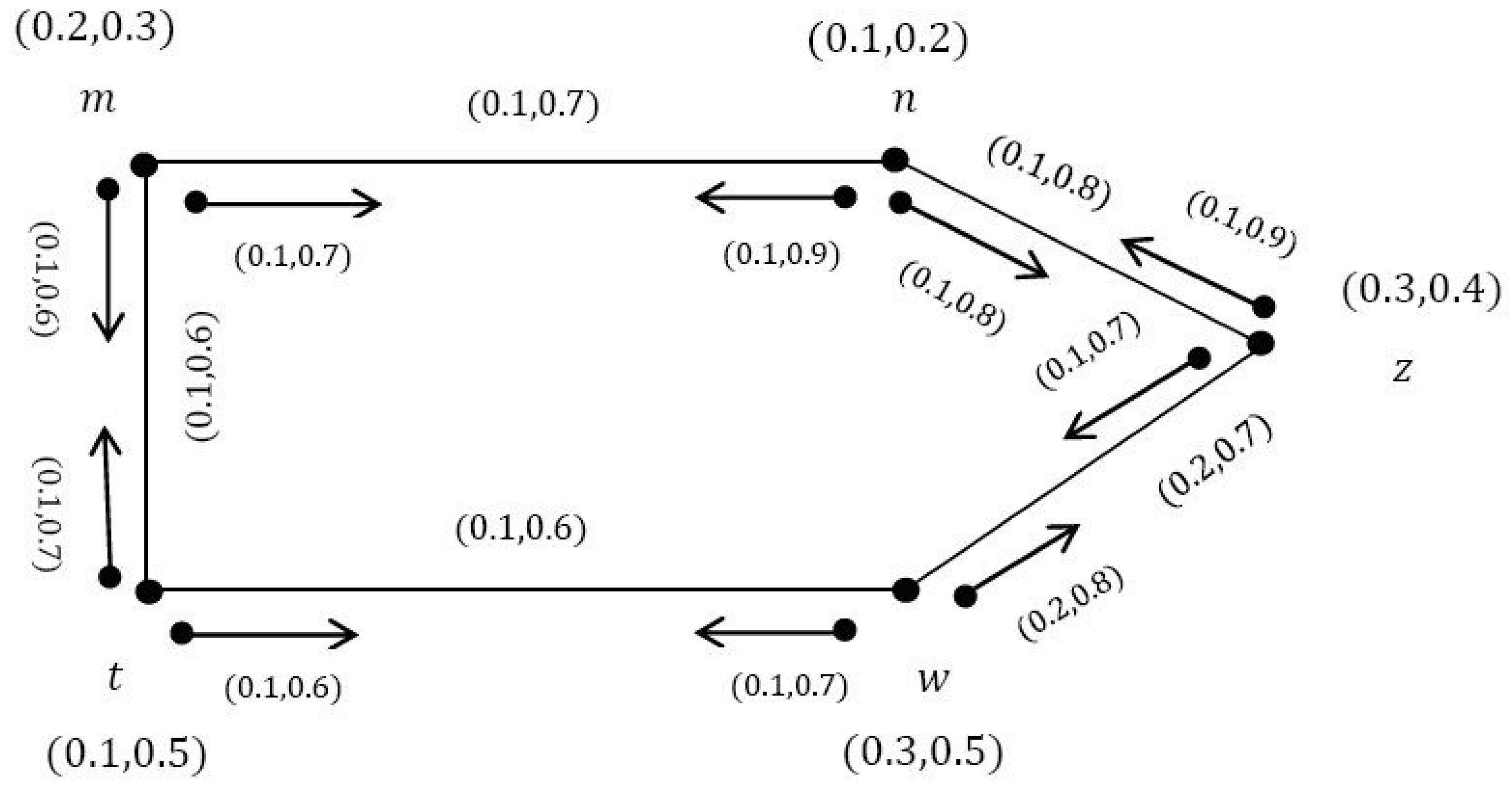
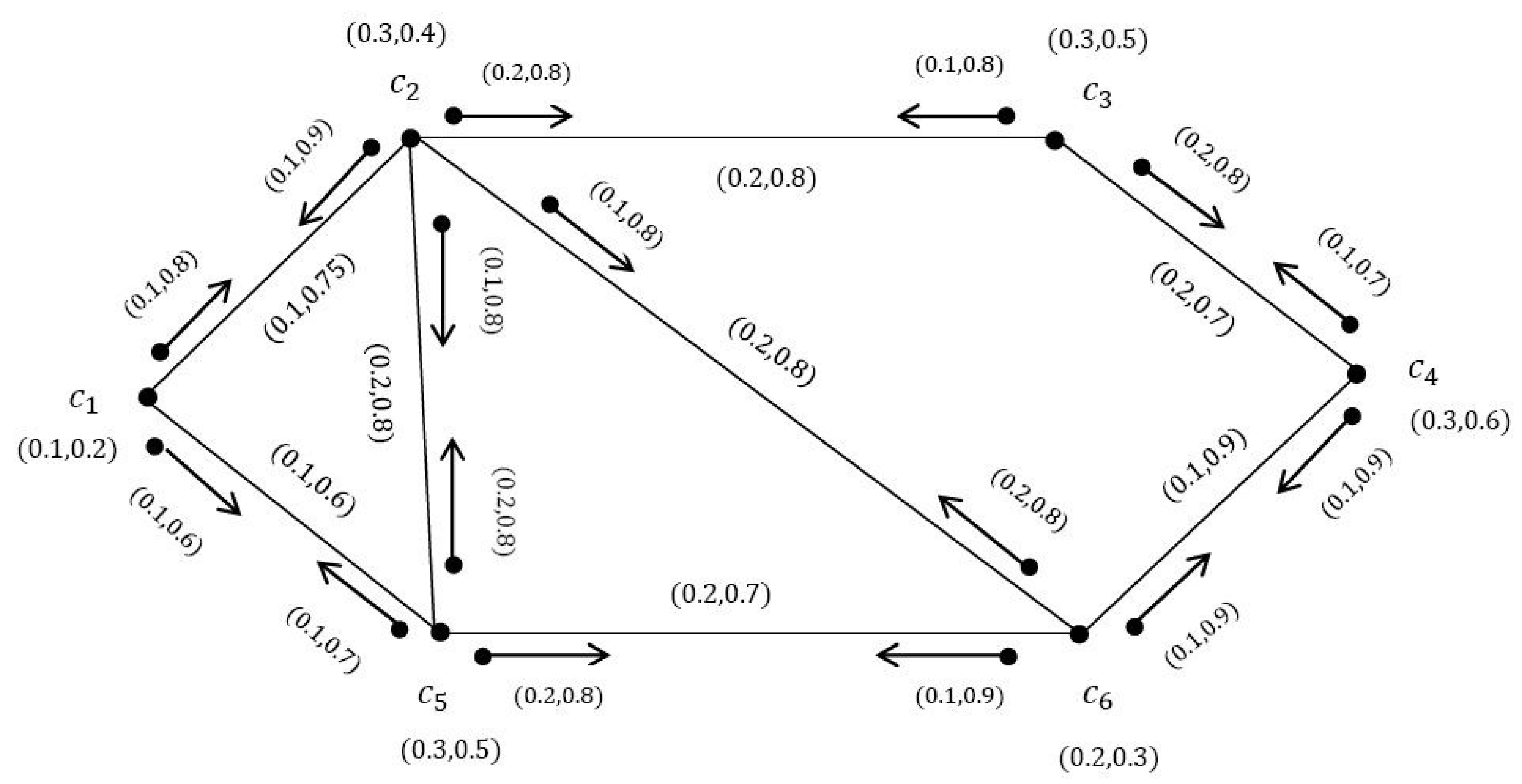
4. Application of VIDS for COVID-19 Testing Facility
Many people today have been infected with Covid-19 virus and in some cases died. Unfortunately, the necessary facilities deficiency in hospitals and clinics has increased the possibility of spreading the virus. Therefore, in this section, we have tried to identify the most effective medical centers with the help of the VIDS to save both cost and time. For this purpose, suppose that there are six different medical diagnostic clinics which are working in a city for conducting COVID-19 tests. Consider the clinics , , , , , and . In VIGs, the vertices show the clinics and edges show the contract conditions between the clinics to share the facilities or test kits. The incidence pairs show the transferring of patients from one clinic to another because of the lack of resources such as kits and doctors. The graph VIDS is the set of clinics which perform the tests independently.
The vertex means that it has of the necessary facilities for diagnosis and treatment of the disease and unfortunately lacks of the necessary equipment. The edge shows that there is only of the interaction and relationship between the two clinics, and due to financial issues and competition, there is on the conflict between them. The dominating sets for the Figure 8 are as follows:
After calculating the cardinality (size) of , we obtain:
It is clear that has the smallest size among other dominating sets, so we conclude that it can be the best choice because, first, there are fewer patients who have the opportunity to transmit the disease to others, and secondly, it will save time and money. Therefore, the government should provide more facilities in the case of COVID-19 disease diagnosis as well as its treatment to clinics so that patients can be identified as soon as possible and do not have to go to different clinics to transmit the disease and spend a lot of money.
5. Conclusions
VIGs are highly practical tools for the study of different computational intelligence and computer science domains. VIGs have many applications in different sciences such as topology, natural networks, and operation research. DSs are a practical interest in several areas. In wireless networking, DSs are used to find efficient routes within ad-hoc mobile networks. They have also been used in document summarization, and in designing secure systems for electrical grids. Therefore, in this paper, we introduced new concepts on VIGs, namely VIDS, isolated vertex, vague incidence irredundant set, and their cardinality related to the domination, etc. At the end, an application of DS for VIG to properly manage the COVID-19 testing facility was presented. In our future work we will investigate the concepts of Energy, spectrum, density, adjacency matrix, degree matrix, Laplacian matrix, and new operations on VIGs and give some applications of spectrum and Energy in VIGs and other sciences.
Author Contributions
“Y.R. and S.K. conceived and designed the experiments; Z.S. performed the experiments; Y.R. and R.C. analyzed the data; Z.S. and L.X. contributed reagents/materials/analysis tools; S.K. wrote the paper.” All authors have read and agreed to the possible publication of the manuscript.
Funding
This work was supported by the National Key R & D Program of China (grant number 2018YFB1005104).
Conflicts of Interest
The authors declare no conflict of interest.
References
- Zadeh, L.A. Fuzzy sets. Inf. Control 1965, 8, 338–353. [Google Scholar] [CrossRef] [Green Version]
- Gau, W.L.; Buehrer, D.J. Vague sets. IEEE Trans. Syst. Man Cybern. 1993, 23, 610–614. [Google Scholar] [CrossRef]
- Rosenfeld, A. Fuzzy Graphs, Fuzzy Sets and their Applications; Zadeh, L.A., Fu, K.S., Shimura, M., Eds.; Academic Press: New York, NY, USA, 1975; pp. 77–95. [Google Scholar]
- Brualdi, R.A.; Massey, J.L.Q. Incidence and strong edge colorings of graphs. Discret. Math. 1993, 122, 51–58. [Google Scholar] [CrossRef] [Green Version]
- Dinesh, T. A Study on Graph Structures. Incidence Algebras and Their Fuzzy Analogous. Ph.D. Thesis, Kannur University, Kerala, India, 2012. [Google Scholar]
- Dinesh, T. Fuzzy incidence graph-an introduction. Adv. Fuzzy Sets Syst. 2016, 21, 33–48. [Google Scholar] [CrossRef]
- Mathew, S.; Mordeson, J.N.; Malik, D.S. Fuzzy Graph Theory; Springer: Cham, Switzerland, 2018. [Google Scholar]
- Mordeson, J.N.; Mathew, S. Fuzzy end nodes in fuzzy incidence graphs. New Math. Nat. Comput. 2017, 13, 13–20. [Google Scholar] [CrossRef]
- Mordeson, J.N.; Mathew, S. Human trafficking: Source, transit, destination, designations. New Math. Nat. Comput. 2017, 13, 209–218. [Google Scholar] [CrossRef]
- Mordeson, J.N.; Mathew, S. Local look at human trafficking. New Math. Nat. Comput. 2017, 13, 327–340. [Google Scholar] [CrossRef]
- Mordeson, J.N.; Mathew, S.; Borzooei, R.A. Vulnerability and government response to human trafficking: Vague fuzzy incidence graphs. New Math. Nat. Comput. 2018, 14, 203–219. [Google Scholar] [CrossRef]
- Ramakrishna, N. Vague graphs. Int. J. Comput. Cogn. 2009, 7, 51–58. [Google Scholar]
- Akram, M.; Naz, S. Energy of pythagorean fuzzy graphs with Applications. Mathematics 2018, 6, 136. [Google Scholar] [CrossRef] [Green Version]
- Akram, M.; Sitara, M. Certain concepts in Intuitionistic Neutrosophic Graph Structures. Information 2017, 8, 154. [Google Scholar] [CrossRef] [Green Version]
- Akram, M.; Naz, S.; Smarandache, F. Generalization of Maximizing Deviation and TOPSIS Method for MADM in Simplified Neutrosophic Hesitant Fuzzy Environment. Symmetry 2019, 11, 1058. [Google Scholar] [CrossRef] [Green Version]
- Borzooei, R.A.; Rashmanlou, H. Ring sum in product intuitionistic fuzzy graphs. J. Adv. Res. Pure Math. 2015, 7, 16–31. [Google Scholar] [CrossRef]
- Borzooei, R.A.; Rashmanlou, H. Domination in vague graphs and its applications. J. Intel-Ligent Fuzzy Syst. 2015, 29, 1933–1940. [Google Scholar] [CrossRef]
- Borzooei, R.A.; Rashmanlou, H. Degree of vertices in vague graphs. J. Appl. Math. Inform. 2015, 33, 545–557. [Google Scholar] [CrossRef]
- Borzooei, R.A.; Rashmanlou, H.; Samanta, S.; Pal, M. Regularity of vague graphs. J. Intell. Fuzzy Syst. 2016, 30, 3681–3689. [Google Scholar] [CrossRef]
- Kosari, S.; Rao, Y.; Jiang, H.; Liu, X.; Wu, P.; Shao, Z. Vague Graph Structure with Application in Medical Diagnosis. Symmetry 2020, 12, 1582. [Google Scholar] [CrossRef]
- Rao, Y.; Kosari, S.; Shao, Z. Certain Properties of Vague Graphs with a Novel Application. Mathematics 2020, 8, 1647. [Google Scholar] [CrossRef]
- Shao, Z.; Kosari, S.; Rashmanlou, H.; Shoaib, M. New Concepts in Intuitionistic Fuzzy Graph with Application in Water Supplier Systems. Mathematics 2020, 8, 1241. [Google Scholar] [CrossRef]
- Shao, Z.; Kosari, S.; Shoaib, M.; Rashmanlou, H. Certain Concepts of Vague Graphs With Applications to Medical diagnosis. Front. Phys. 2020, 8, 3–57. [Google Scholar] [CrossRef]
- Samanta, S.; Pal, M. Fuzzy k-competition graphs and pcompetition fuzzy graphs. Fuzzy Inf. Eng. 2013, 5, 191–204. [Google Scholar] [CrossRef]
- Samanta, S.; Akram, M.; Pal, M. m-step fuzzy competition graphs. J. Appl. Math. Comput. 2014. [Google Scholar] [CrossRef]
- Samanta, S.; Pal, M. Irregular bipolar fuzzy graphs. Int. J. Appl. Fuzzy Sets 2012, 2, 91–102. [Google Scholar]
- Samanta, S.; Pal, M. Some more results on bipolar fuzzy sets and bipolar fuzzy intersection graphs. J. Fuzzy Math. 2014, 22, 253–262. [Google Scholar]
- Rashmanlou, H.; Borzooei, R.A. Vague graphs with application. J. Intell. Fuzzy Syst. 2016, 30, 3291–3299. [Google Scholar] [CrossRef]
- Rashmanlou, H.; Samanta, S.; Pal, M.; Borzooei, R.A. A study on bipolar fuzzy graphs. J. Intell. Fuzzy Syst. 2015, 28, 571–580. [Google Scholar] [CrossRef]
- Rashmanlou, H.; Borzooei, R.A. Product vague graphs and its applications. J. Intell. Fuzzy Syst. 2016, 30, 371–382. [Google Scholar] [CrossRef]
- Rashmanlou, H.; Jun, Y.B.; Borzooei, R.A. More results on highly irregular bipolar fuzzy graphs. Ann. Fuzzy Math. Inform. 2014, 8, 149–168. [Google Scholar]
- Somasundaram, A.; Somasundaram, S. Domination in fuzzy graph—I. Patter Recognit. Lett. 1998, 19, 787–791. [Google Scholar] [CrossRef]
- Parvathi, R.; Thamizhendhi, G. Domination in intuitionistic fuzzy graph, Proceedings of the14th International Conference on Intuiyionistic Fuzzy Graphs. Notes Intuit. Fuzzy Sets 2010, 16, 39–49. [Google Scholar]
- Nagoorgani, A.; Mohamed, S.Y.; Hussain, R.J. Point set domination of intuitionistic fuzzy graphs. Int. J. Fuzzy Math. Arch. 2018, 7, 43–49. [Google Scholar]
- Talebi, Y.; Rashmanlou, H. New concepts of domination sets in vague graphs with applications. Int. J. Comput. Sci. Math. 2019, 10, 375–389. [Google Scholar] [CrossRef]
Figure 1.
Vague graph G.

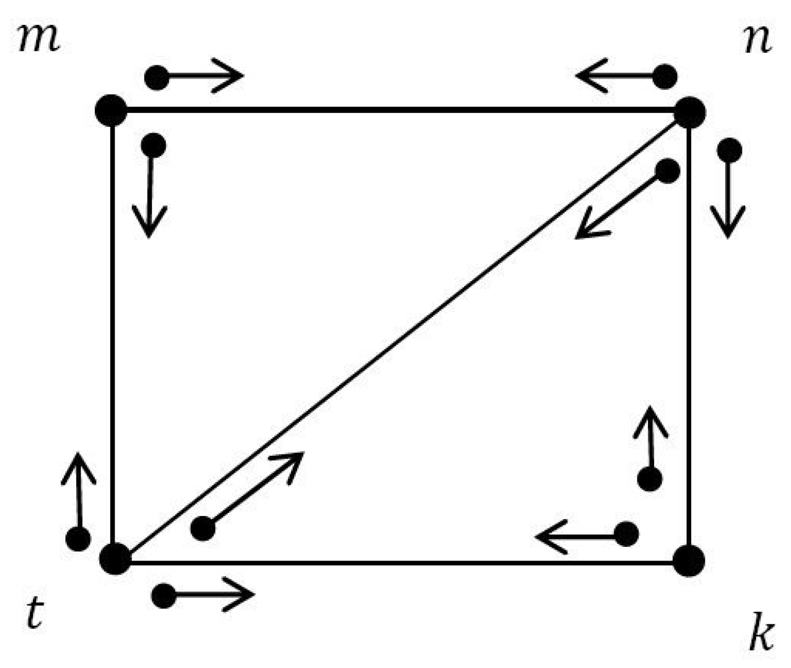
Figure 2.
Incidence graph .

Figure 3.
VIG ζ.

Figure 4.
VIG ζ.

Figure 5.
Complete VIG ζ.

Figure 6.
VIG ζ.

Figure 7.
A VIG with all valid edges.

Figure 8.
VIG G.


Table 1.
Some basic notations.
| Notation | Meaning |
|---|---|
| Vague Incidence Graph | |
| FG | Fuzzy Graph |
| VG | Vague Graph |
| FIG | Fuzzy incidence Graph |
| VIG | Vague Incidence Graph |
| DS | Dominating Set |
| VS | Vague Set |
| VIDS | Vague Incidence Dominating Set |
| VIIS | Vague Incidence Irredundant Set |
| VDS | Vague Dominating Set |
Publisher’s Note: MDPI stays neutral with regard to jurisdictional claims in published maps and institutional affiliations. |
© 2020 by the authors. Licensee MDPI, Basel, Switzerland. This article is an open access article distributed under the terms and conditions of the Creative Commons Attribution (CC BY) license (http://creativecommons.org/licenses/by/4.0/).
Share and Cite
MDPI and ACS Style
Rao, Y.; Kosari, S.; Shao, Z.; Cai, R.; Xinyue, L. A Study on Domination in Vague Incidence Graph and Its Application in Medical Sciences. Symmetry 2020, 12, 1885. https://doi.org/10.3390/sym12111885
AMA Style
Rao Y, Kosari S, Shao Z, Cai R, Xinyue L. A Study on Domination in Vague Incidence Graph and Its Application in Medical Sciences. Symmetry. 2020; 12(11):1885. https://doi.org/10.3390/sym12111885
Chicago/Turabian StyleRao, Yongsheng, Saeed Kosari, Zehui Shao, Ruiqi Cai, and Liu Xinyue. 2020. "A Study on Domination in Vague Incidence Graph and Its Application in Medical Sciences" Symmetry 12, no. 11: 1885. https://doi.org/10.3390/sym12111885
Note that from the first issue of 2016, this journal uses article numbers instead of page numbers. See further details here.