
Ensemble Prediction Approach Based on Learning to Statistical Model for Efficient Building Energy Consumption Management


1
Department of Computer Engineering, Jeju National University, Jejusi 63243, Korea
2
Department of Computer Science, COMSATS University Islamabad, Attock Campus 43600, Pakistan
*
Author to whom correspondence should be addressed.
Symmetry 2021, 13(3), 405; https://doi.org/10.3390/sym13030405
Submission received: 21 January 2021
/
Revised: 22 February 2021
/
Accepted: 25 February 2021
/
Published: 2 March 2021
Abstract
:With the development of modern power systems (smart grid), energy consumption prediction becomes an essential aspect of resource planning and operations. In the last few decades, industrial and commercial buildings have thoroughly been investigated for consumption patterns. However, due to the unavailability of data, the residential buildings could not get much attention. During the last few years, many solutions have been devised for predicting electric consumption; however, it remains a challenging task due to the dynamic nature of residential consumption patterns. Therefore, a more robust solution is required to improve the model performance and achieve a better prediction accuracy. This paper presents an ensemble approach based on learning to a statistical model to predict the short-term energy consumption of a multifamily residential building. Our proposed approach utilizes Long Short-Term Memory (LSTM) and Kalman Filter (KF) to build an ensemble prediction model to predict short term energy demands of multifamily residential buildings. The proposed approach uses real energy data acquired from the multifamily residential building, South Korea. Different statistical measures are used, such as mean absolute error (MAE), root mean square error (RMSE), mean absolute percentage error (MAPE), and score, to evaluate the performance of the proposed approach and compare it with existing models. The experimental results reveal that the proposed approach predicts accurately and outperforms the existing models. Furthermore, a comparative analysis is performed to evaluate and compare the proposed model with conventional machine learning models. The experimental results show the effectiveness and significance of the proposed approach compared to existing energy prediction models. The proposed approach will support energy management to effectively plan and manage the energy supply and demands of multifamily residential buildings.
1. Introduction
In recent times, a considerable amount of energy consumption is attributed to residential buildings. owing to a high consumption share of the building sector worldwide has turned into an undefined energy sink. The residential building sector worldwide consumes about 40% of energy consumption [1] comparative to industrial and commercial sectors. Increased electric consumption leads to increased wastage and the least energy savings. Wasting a scarce resource such as electricity is a substantial threat to economy and sustainability of a country. Moreover, electricity generated through fossil fuels such as coal and natural gas produce emissions, which become the leading causes of greenhouse gas emissions and global warming [2]. Achieving building energy efficiency can assist authorities in minimizing and controlling the carbonization of the energy sector. Therefore, energy modeling for the buildings sector is a dire need of the current hour to analyze the building electric consumption with respect to improving building design, achieving control system optimization, reducing energy wastage, facilitating stable grid operations, and improving decision power through development of efficient electricity consumption prediction models. The critical aspect of electricity is that its production, transmission, and distribution happens in real-time, and there is no mechanism to store it; furthermore, instantaneous production of electric energy is impossible as the production process requires time and effort; therefore, accurate energy consumption forecasts are needed to avoid over and underproduction of electricity.
Electricity consumption prediction is a substantial part of power system planning and operation of electric utility companies. Planning facilitates an electric utility to make informed decisions about future requirements. Prediction assists building owners and electric utility companies by provisioning future electric consumption likelihood to the planning department, which further implements specific planning strategies for effective management. Electric consumption prediction estimates future electric consumption based on the already recorded consumption data and some influencing variables such as weather and occupant comfort indexes, etc. Electric utility companies need different types of consumption forecasts to satisfy their vast business needs. Electric consumption forecasts are a major concern of power authorities to avoid blackouts and power-outages; moreover, for efficient financial planning and smooth electricity transmission, distribution, and generation. However, electric consumption forecasting is a challenging task due to various influencing factors such as outdoor weather conditions, size of the building, number of occupants, the economic state and comfort index of the occupant, the use of heating, ventilation, and air conditioning components (HVAC), operating schedules, and energy usage pattern of the occupant [3,4]. Electric energy consumption prediction is comprised of various temporal scales to analyze consumer electricity demands, such as hourly, sub-hourly, daily, weekly, monthly, yearly, and seasonally (Summer, Winter, and Fall) [5]. Therefore, it is beneficial to utilize data analytics to process and analyze the hidden characteristics of electrical energy consumption data that is essential for understanding the energy demands of multifamily residential buildings.
Time series data are widely used to forecast the future consumption of electricity. It can be defined as a chronological sequence of samples on a pattern of interest [6]. As we discussed earlier, the consumption demands of electricity depend on different time series patterns, such as hourly, daily, weekly, etc. Therefore, it is required to unearth the time-series patterns to analyze consumer demands. Nowadays, Data Mining (DM) techniques are widely used to discover essential characteristics from a large data scale [7]. It is an effective process of discovering useful patterns and hidden trends from electricity consumption data, which is important for energy management to plan electricity demands and supply [8]. The DM techniques can examine and analyze a massive amount of time series data through analytical reasoning models for extracting useful characteristics and insights from complex consumption data that is an indispensable part of efficient energy management and for devising strategies to plan, control, and coordinate energy supply and consumption demands.
Recently, machine learning (ML) algorithms are widely used by the researchers to build intelligent inference models based on discovered characteristics using DM techniques to forecast time series data. ML algorithms are employed by many researchers to develop intelligent models in various domains, such as computer vision [9], business intelligence, pattern recognition [10], navigation systems [11], decision-making systems [12], etc. ML-based techniques are robust to build intelligent inference models based on historical electric consumption data and discover underlying characteristics to derive a conclusion. Deep learning models have gained enormous attention in recent times and have successfully produced state-of-the-art results. It is an active technology employed in various research areas like computer vision, bioinformatics, energy forecasting, health care systems, speech recognition, etc. [13]. Deep learning models can learn representations from structured and unlabeled data using multilayered neural networks. Comparative to traditional models, deep learning models offer better prediction performance because of varying layers and abstraction levels [14]. Deep neural networks are based on stochastic optimization, like Long Short Term Memory Recurrent Neural networks (LSTM-RNN). Recurrent Neural Networks (RNN) possess an internal memory block that aids learning from past experiences; moreover, it comprise of looping structures from output to input nodes. Recurrent nets are sequence-based models that are capable of tackling dependencies between consecutive time steps. RNN can be considered a replicating structure of the same network, with each copy passing a message to the next node [15]. However, practically, RNN faces difficulties in learning long-range dependencies. LSTM neural networks offer a solution to such problems by providing feedback connections. LSTM is highly productive and provides a solution to various domains like prediction, data processing, and classification, etc. LSTM is a special variant of RNN that has self-connecting hidden layers and gating structure and is efficient at handling long term dependencies with better controllability [16]. The LSTM based prediction model learns from past data and predicts future outcomes. However, adapting to dynamic conditions associated with intricate electric consumption patterns is a challenging task. To cope with this issue, researchers have realized the potential of employing KF to improve the performance of prediction models [17]. Kalman filter is a statistical algorithm that only requires previous state information (predicted state) and noise measurements to predict optimal, unbiased actual system state.
The major contributions of the proposed work are listed as follows:
- Provide different time-series analysis of energy consumption data of multifamily residential buildings, South Korea, to highlight hidden insights and characteristics for stakeholders to devise effective policies.
- Integration of deep learning and statistical models to forecast short-term energy consumption using time-series data collected from multifamily residential buildings, South Korea.
- Experimental results demonstrate that the proposed ensemble prediction approach produces better generalization and outperforms standalone models, such as LSTM and KF.
- Comparative analysis is also given to highlight the significance of the proposed model compared to standalone models.
The rest of the paper is summarized as follows: Section 2 presents the related works; Section 3 presents methodology of the proposed ensemble prediction model based on LSTM and KF using time-series electricity consumption data of multi-family buildings. Section 4 presents detailed time-series analysis to investigate hidden characteristics of electricity consumption data. In Section 5, prediction approaches are discussed. In Section 6, we present the implementation environment, experimental, and performance analysis results. Section 7 concludes the paper with possible future directions.
2. Related Work
This section presents existing work related to energy prediction models and provides an overview of state-of-the-art methods applied to the domain of electric consumption forecasting. Previously, a variety of electric consumption prediction models have been developed using various software packages like Ecotect [18], Energy-plus [19], DOE2 [20], IES [21], etc. This type of modeling requires detailed knowledge of the building’s structural, thermal, and material properties. Additionally, such methods utilize engineering models to calculate the future electric consumption of a building. However, such detailed information about a building is unavailable at the time of prediction, and, if obtained, it is difficult to validate it, creating a hindrance in prediction performance and accuracy. Due to the complexities associated with electric consumption prediction, particularly low accuracy and deteriorated prediction performance, employing simulation tools is therefore not the right choice for energy prediction. To overcome the limitations in existing solutions, there is a growing interest in data-driven approaches [22]. Data-driven models learn from past electric consumption data and predict future consumption based on past consumption patterns [23]. With the advent of Smart Metering Infrastructure (SMI) in recent years, data-driven approaches are successfully applied to this domain due to fast computational power and improved prediction performance.
Data-driven methods applied to energy consumption prediction are generally developed using statistical and artificial intelligence (AI) methods. Statistical methods build probabilistic models based on historical data as their internals are known, making it easy to understand the internal processes. These statistical models include Exponential Smoothing [24], Auto-regressive Moving Average [25], Regression Analysis [26], Stochastic Time Series Modeling [27], etc. Statistical methods are uncomplicated and simpler in implementation yet they cannot handle intricate nonlinear electric consumption patterns. In contrast, ML-methods are robust and effective in handling shortcomings, as mentioned above. Commonly used AI methods include artificial neural networks (ANN), deep neural networks (DNN), support vector machine (SVM), fuzzy inference systems (FIS), expert systems (ES), etc. ANN based studies include work from Chae et al. [28]. The authors forecasted electric consumption of an office building using ANN and Bayesian Regularization; comparing ANN and nine other methods and experimental results proved that ANN along Bayesian regularization outperformed all other methods. Quilumba et al. [29] applied neural networks and clustered data from smart meters to forecast intraday load at a system level. In [30], the authors proposed a hybrid model to integrate physical and SVM models to predict short-term electric consumption. Paudel et al. [31] employed SVM to forecast the overall (heating and cooling) energy consumption of a residential building. Refs. [32,33] successfully applied fuzzy inference systems by mapping the relationship between electric consumption and variables affecting it. Although ANN is one of the popular techniques, it is unable to achieve lower error due to over fitting, issues in training, inappropriate generalization, and weakness of back propagation.
Recently, deep learning has become the most popular approach due to its application in several areas due to its successful application in various research areas: natural language translation, picture captioning, pattern recognition, and, most importantly, sequence learning. Deep learning consists of several architectures like long short term memory (LSTM), recurrent neural network (RNN), convolution neural network (CNN), and deep belief network (DBN) [34,35,36]. Among the ML methods employed in energy consumption prediction, DNN methods have proven effective and robust to handle nonlinear time series problems [4]. Deep networks are successfully applied to energy forecasting and achieved the best results compared to previous methods. Deep learning uses the concept of stochastic optimization for performing ML tasks. Multiple layers of a neural network are stacked over each other to improve results and learning ability; they are provided with different abstraction levels [14]. DL methods are a suitable choice to overcome the problems that existed in previous methods because these methods can model complex functions.
Deep networks are successfully applied to energy forecasting and achieved the best results compared to previous methods. Debinec et al. [37] employed a deep belief network to forecast daily electric consumption in Macedonia by stacking multiple Restricted Boltzmann Machine (RBM) layers. Mocanu et al. [38] introduced another deep learning method called a conditional restricted Boltzmann machine for predicting the load of a residential building for a single meter and achieved better performance compared to ANN and SVM. El-shark [39] employed radial basis recurrent neural networks with multilayer perceptron and parallel artificial neural networks. In [40], the authors used an ensemble deep belief networks to predict electric consumption using three different time-series data sets. In [41], the authors introduced a novel approach known as hybrid quantized elman neural network (HQENN) to predict future hourly load consumption. Ertugrul et al. [42] presented a novel prediction approach based on an RNN and extreme learning machine (ELM). The proposed work aims to predict electricity consumption to facilitate policy makers formulate policies according to electric consumption prediction statistics. Mandal et al. [43] applied basic ANN to forecast electric consumption by clustering similar days consumption profile using hourly electric consumption and temperature as an input. Similarly, in [44], the authors employed a novel sequence-based LSTM (S-LSTM) to predict electric consumption and achieved promising results compared to simple LSTM. In [45], the authors proposed a novel deep learning-based framework for improving the prediction accuracy of short term electric load forecasting. Another study employed CNN and deep CNN along with LSTM.The authors [46] formulated a novel approach based on a hybrid of ANN with an evolutionary algorithm called as Follow The Leader (FTL) to predict short-term load. The proposed hybrid scheme provides optimal parameter tuning for neural networks, thus improving learnability and predictive performance. In [47], the authors presented a sister forecasters-based short-term load forecasting approach. The proposed framework presented a family of prediction models called sisters having the same model structures but a different variable selection process. The authors proposed a bi-directional LSTM model to predict short term load of electricity in smart grid to support peer-to-peer energy trading [48].
Several studies proposed statistical-based prediction models to predict short-term electricity consumption of residential buildings. In [49], the authors proposed a Kalman filter (KF) based method for short term electric load forecasting. The proposed method employs state-space combined with fuzzy rule-based logic. Experiments conducted with a real dataset comprised of load and weather data demonstrating MAPE of 0.7 percent. Similarly, in [50], the authors proposed an hourly load forecasting approach employing Kalman filter and the adaptive neural-fuzzy inference system (ANFIS). In [51], the authors also presented a Kalman Filter -based method to forecast short term electric load forecasting for power systems. Experimental results suggested that KF is an excellent choice for six hours ahead of forecasting. The authors proposed a novel electric load forecasting and analysis framework based on ensemble KF and multiple regression method [52]. This approach was based on state-space load modeling and ensemble Kalman filtering for state estimation. In [53], the authors developed a framework for monthly load forecasting using a hybrid empirical mode decomposition and state-space model. The proposed work optimizes the parameters of state-space models using Kalman Filter.
Table 1 summarizes the existing prediction models proposed by different researchers to predict short-term energy load to facilitate policymakers.
To the best of the authors’ knowledge, all of the mentioned prediction models attempted to forecast short-term energy consumption using DL or statistical models. None of the aforementioned studies attempted to combine DL and statistical techniques to predict short-term energy consumption to facilitate energy strategists. Therefore, it is the first-ever attempt to combine LSTM and KF to predict short-term electricity consumption using real data of multi-family residential buildings, South Korea. The combination of LSTM and KF can achieve superior performance, fast convergence, and the least error consumption prediction. The proposed ensemble prediction model will facilitate energy policymakers to control and plan electricity demands and supply.
3. Proposed Ensemble Prediction Approach Based on Learning to Statistical Model
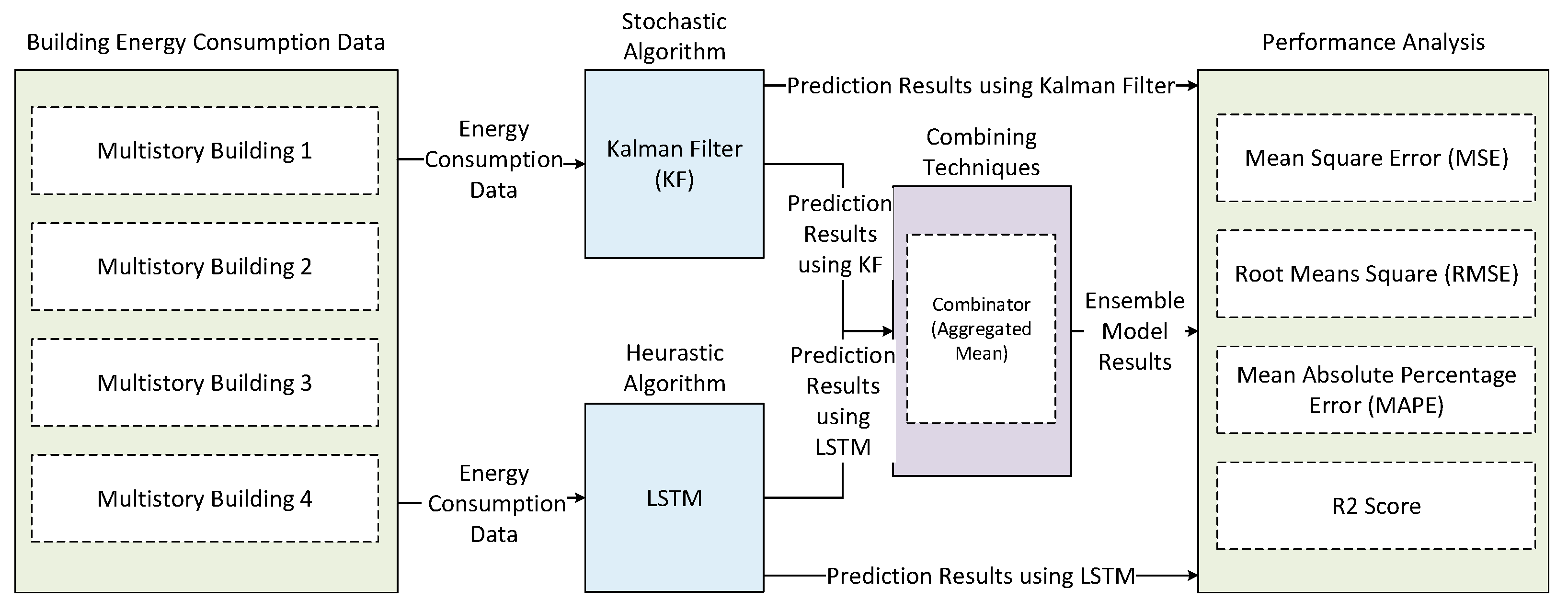
This section presents a proposed ensemble prediction approach based on learning to statistical model in order to accurately predict electric consumption requirements. Efficient building energy management requires accurate electric consumption prediction. Noisy sensor readings, weather changes, and variability in occupant energy use behavior makes electric consumption prediction a challenging task and sometimes results in poor prediction accuracy. Traditional methods are not able to get the desired level of accuracy and suffer from over fitting; these methods learn the data patterns from scratch, thus creating a complexity in correlation among the variables. All of these issues can be solved by an ensemble sequential learning to statistical model. Therefore, we proposed an ensemble learning to statistical (LSTM-Kalman Filter) prediction model. The architecture of the proposed ensemble model is depicted in Figure 1. Figure 1 shows building electric consumption data along with temperature and humidity being fed to both stochastic (LSTM) and heuristic (Kalman filter) algorithms. The input features are electric consumption for past k sequences, time stamp, temperature, and humidity. Each day consists of 24 hourly readings along with the other parameters, making a 27-dimensional sample space. Before training the models, the data are preprocessed and normalized to get better prediction accuracy. After data preprocessing, the data are fed to the training algorithms to get prediction results. After getting prediction results, we applied the aggregated mean as a combining mechanism to produce final ensemble model results. In this study, we employed LSTM as the base level model for training; afterwards, KF acts as a meta-model and uses the output of base model as an input for training. Hence, the electric consumption prediction produced by LSTM is used as features for the stochastic model. After testing the model with the test set, performance will be evaluated. In case of poor prediction performance, the models will be retrained. Model evaluation involves the evaluation of the prediction model using standard evaluation metrics such as MAPE, MSE, RMSE, and R2 score. Furthermore, our proposed ensemble learning to statistical prediction model has the ability to estimate states of a dynamically changing system.
Proposed Ensemble Prediction Model Architecture
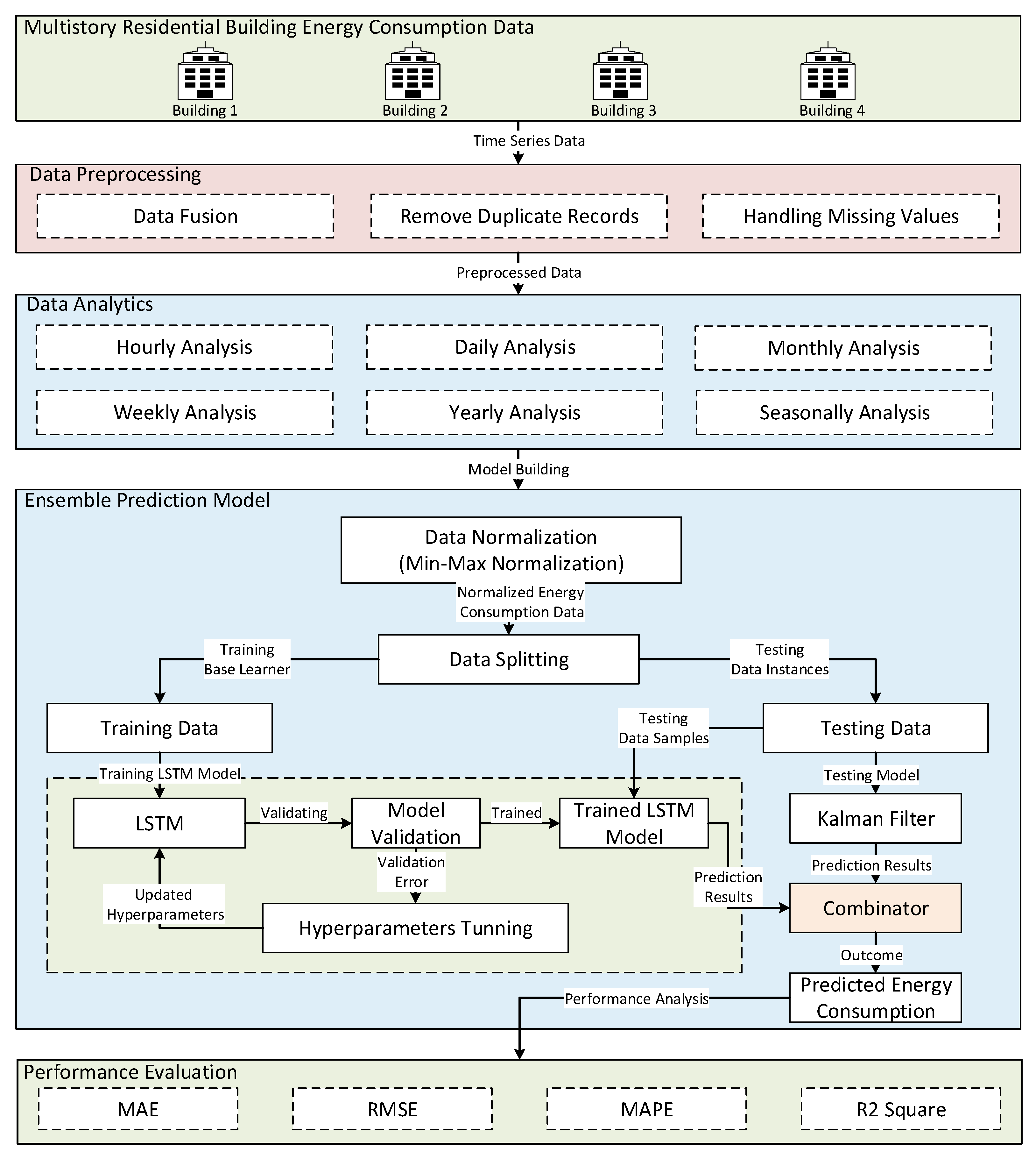
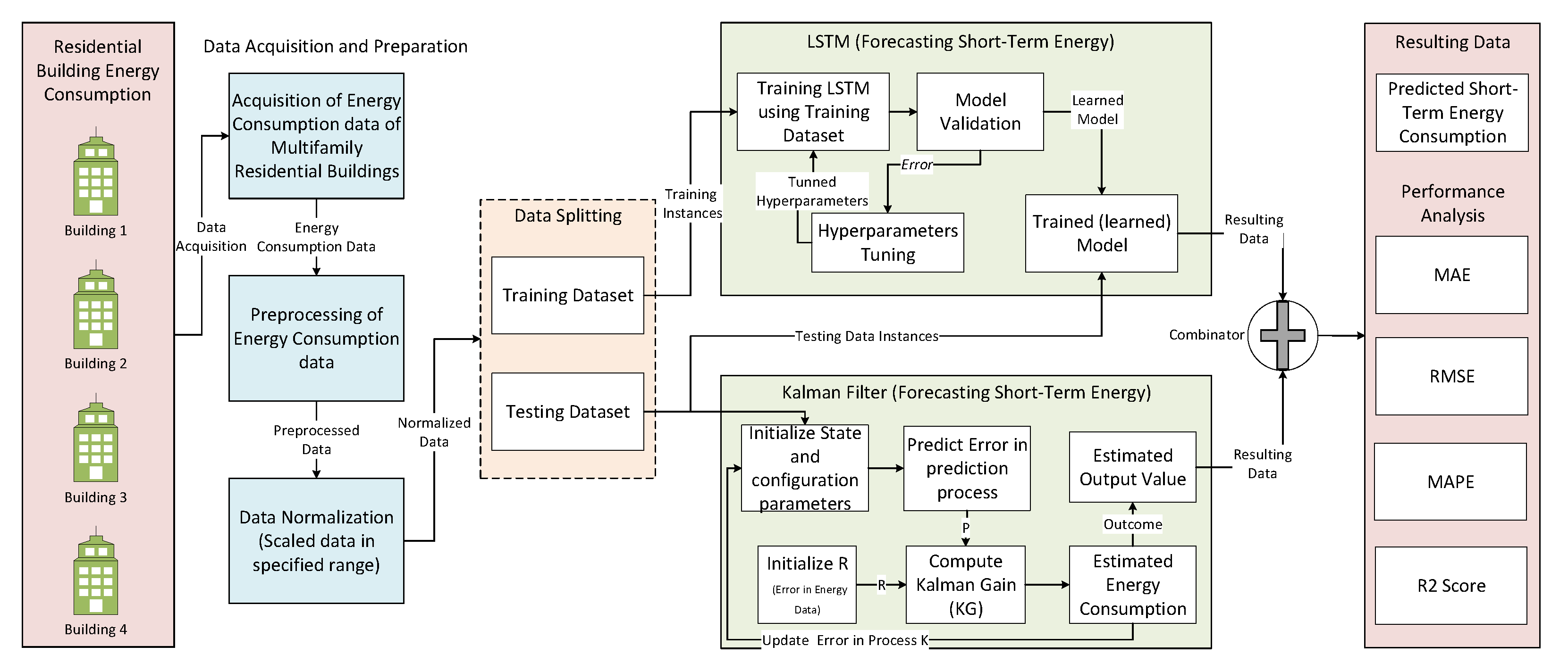
This subsection presents architecture of the proposed ensemble prediction model. The following Figure 2 presents the architecture of the proposed ensemble prediction model to predict short-term demands of energy consumption for residential buildings. The proposed model architecture consists of the following steps: acquisition of residential energy consumption data, preprocessing of energy consumption data, time-series analysis (including hourly, daily, weekly, monthly, and seasonally), data normalization, data splitting into training and testing subsets, training and testing of ensemble model based on LSTM and Kalman Filter, and performance evaluation.
The dataset consists of electric consumption data corresponding to the timespan of one year starting from 1 January 2010 to 31 December 2010 along with time stamp information. Data are collected using smart meters, and weather data are provided by KMA. In the preprocessing step, missing values are handled, duplicated values are removed, and data fusion is done in order to help the model achieve better accuracy and improvable model training. Next, we performed time-series analysis to get a clearer picture of the collected data, and some basic statistics are calculated to get the insight of the data distribution. In this paper, we performed different time-series analysis, such as hourly, daily, weekly, yearly, and seasonal data analysis, to analyze hidden insights of the given data. Due to a large amount of consumption data, data normalization is done to make sure weights and biases achieve convergence. In the data normalization step, we use the min-max normalization technique to normalize data in some defined range [0,1] to avoid data skewness. As LSTM is sensitive with regards to input scaling, therefore we normalized the data through scaling the features using min-max normalization. The data splitting step is used to divide the given data into training and testing sets. In this paper, we use a standard split ratio of 70/30; 70% of data instances are used for the training model and remaining data/days are fixed for validation and testing. The next step is used to discuss an ensemble prediction model based on LSTM and KF. LSTM acts as a heuristic learner which learn patterns from hourly electric consumption to predict short-term energy consumption demands of the residential buildings, whereas KF acts as a stochastic algorithm that is used to process the training filtering problem and works by estimating states by the reduction of average distance between data and its curve, although it only stores the result computed from the previous step. Besides being beneficial, another aspect of the Kalman Filter is that it relies on the dynamic model because reason because LSTM is used as they both complement each other to overcome certain issues that exist in each of them separately. An aggregated mean is used to combine prediction results of the LSTM and KF. Integration of LSTM and KF not only eliminates its dependency on the dynamic model but also facilitates learning from the data. Moreover, it also increases the ability of electric consumption prediction in the Kalman filter. Finally, we use different performance measures to evaluate the performance of the proposed ensemble prediction model, such as MSE, RMSE, MAPE, and R2 Score.
4. Time Series Analysis of Building Energy Consumption Data
This section presents time-series analysis to investigate hidden insights of the energy consumption data. The time series analysis of building electric consumption has enabled us to analyze the load signals with respect to time as a series of hourly, daily, weekly, and seasonal predictions.
4.1. Residential Building Energy Consumption Data
This study is conducted on a real dataset consisting of electric consumption data collected from a residential building to forecast the electric consumption. The acquired dataset consists of four residential multi-family buildings. Each residential building consists of 33 floors. Data have been recorded on an hourly basis for each apartment. Each building has different families (having unique characteristics) residing in each apartment. This dataset is recorded at an hourly temporal granularity. Data are collected using smart meters; each apartment has one smart meter to record consumption. The input features consists of historical electric consumption for past k sequences, and time stamp. Each day consists of 24 hourly consumption readings and the other inputs making a 25-dimensional sample space. The dataset has electric consumption data corresponding to a period of one year starting from 1 January 2010 to 31 December 2010. Data aggregation is done at the building level. The collected data were in the form of XML files converted into CSV for experimental use.
4.2. Data Preprocessing/Cleaning
Data preprocessing is the most vital step for achieving high accuracy, the electric consumption data and weather related data suffer from missing values. Missing values if not dealt can be very problematic. Therefore, we filled the missing values by taking into account adjacent hourly and daily values related to that specific input feature. In the next phase, we remove the duplicate records to avoid over fitting of the model; first, we detect them using a technique from pandas library and then drop the duplicated values. Then, we fused the data to produce a collective integrated data from multiple files for producing lower error in results. For further preprocessing, we assumed that the data have noise as many factors may influence the reading. Moving average is considered one of the widely used methods to deal with time-series data abnormalities [54]. Hence, we employed moving average to deal with abnormalities. Moving average is calculated as follows in Equation (1):
where output signal is represented by y, x is the input, and M represents how many points there are on average. This method use load average values taken from the same days and same time in a sequence on similar to same day same time in previous weeks.
4.3. Time Series Analysis
This subsection presents time-series analysis to get a clearer picture of the collected data, and some basic statistics are calculated to get the insight of the data distribution. Moreover, time-series analysis is used to gain a perspective over past outcomes and forecasting future values and analyzing fluctuations in sequence data.
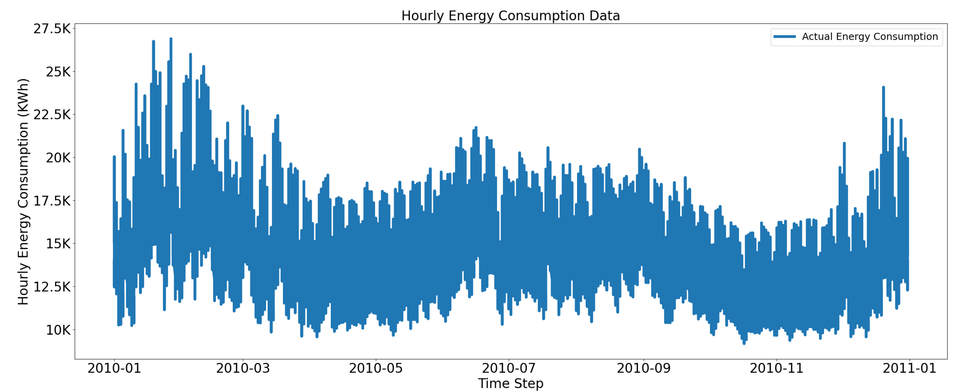
Figure 3 depicts hourly electric consumption data prior to data normalization. The highest and lowest range for consumption is depicted in Figure 3. Hourly data analysis is used to reveal hourly load peaks; therefore, it is important for policy makers to plan and control energy supply and demands. The hourly data consumption fluctuates between 10,000 KWh and 27,000 KWh for all four multi-family residential buildings.
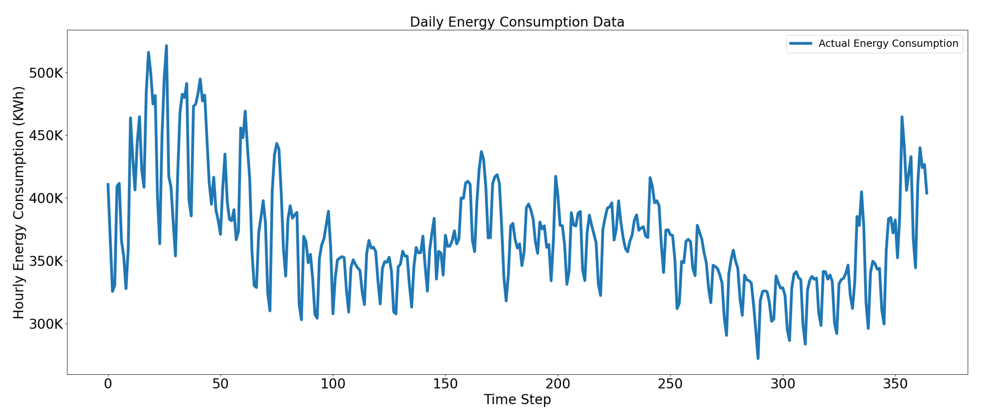
In Figure 4, we can see fluctuations in daily and weekly electric consumption of a building, weekdays start from Monday and end on Friday, social and working activities are on the rise during the week day; likewise, the consumption increases. Therefore, we incorporated holiday label features to separate weekday consumption from non-week days. Residential load is dynamic in nature, and multi-storied residential buildings have their own schedule of operations, comfort levels, and occupant consumption behavior. This is why electric consumption varies as we progress along various time steps. Moreover, external weather conditions also greatly impact the consumption and performance of the model, which can be seen clearly in the daily consumption representation.
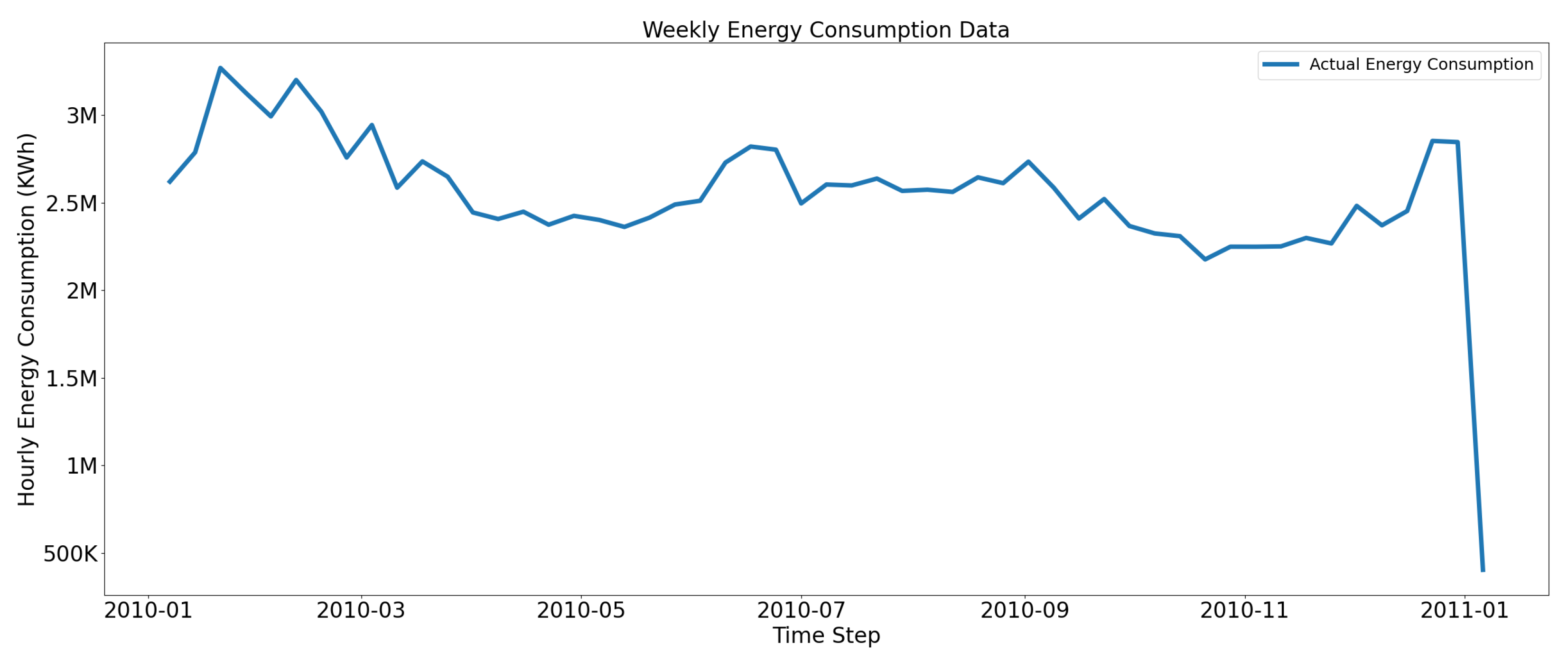
Similarly, Figure 5 presents weekly analysis to visualize energy consumption data. It can be observed that the weekly building energy consumption is more stable compared to commercial context where there is a rise during weekdays due to fixed operating hours, and the consumption decreases on the weekend. However, the residential context shows a slight increase during the daytime, and the curve flattens at night due to personalized energy use and occupants’ comfort levels.
Likewise, Figure 6 presents monthly percentage analysis of electric energy consumption data. It clearly shows the impact of the sparse yet uniform pattern in the monthly energy consumption. It can be observed that the energy consumption requirements for January are high as compared to other months.
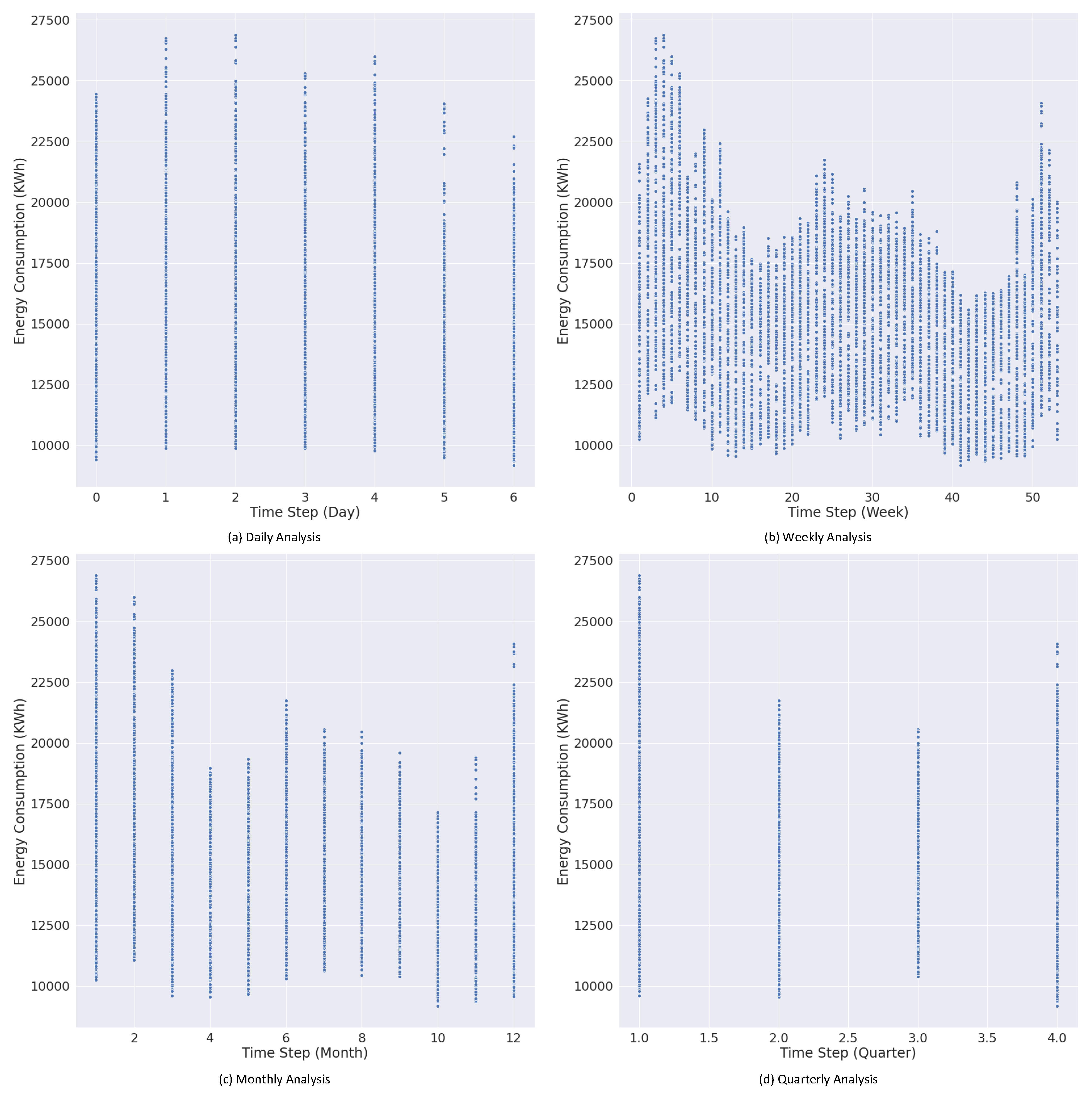
Figure 7 depicts the time series trends of electric energy consumption. Figure 7a presents the daily analysis of electric consumption, and the analysis shows a uniform pattern in the daily consumption with majority values lying between 22,500 and 25,000 KWh. Figure 7b presents how electric consumption is distributed throughout the week. The weekly patterns show some variations in consumption patterns due to weekends and holidays; hence, the peak load hours and off-peak hours have caused fluctuations in electricity consumption trends. The monthly prediction analysis shows variations in consumption due to seasonal variations. During the spring and autumn seasons, electricity consumption is lower due to the limited need for heating and cooling. Similarly, during extreme weather conditions, the need for heating and cooling with respect to the occupant comfort levels is reflected in the monthly analysis. The quarterly analysis shows the electricity consumed during the first, second, third, and fourth quarter. Consumption patterns are high in the first and fourth quarters, which show the high consumption share and the rest of all average consumption behavior quarterly.
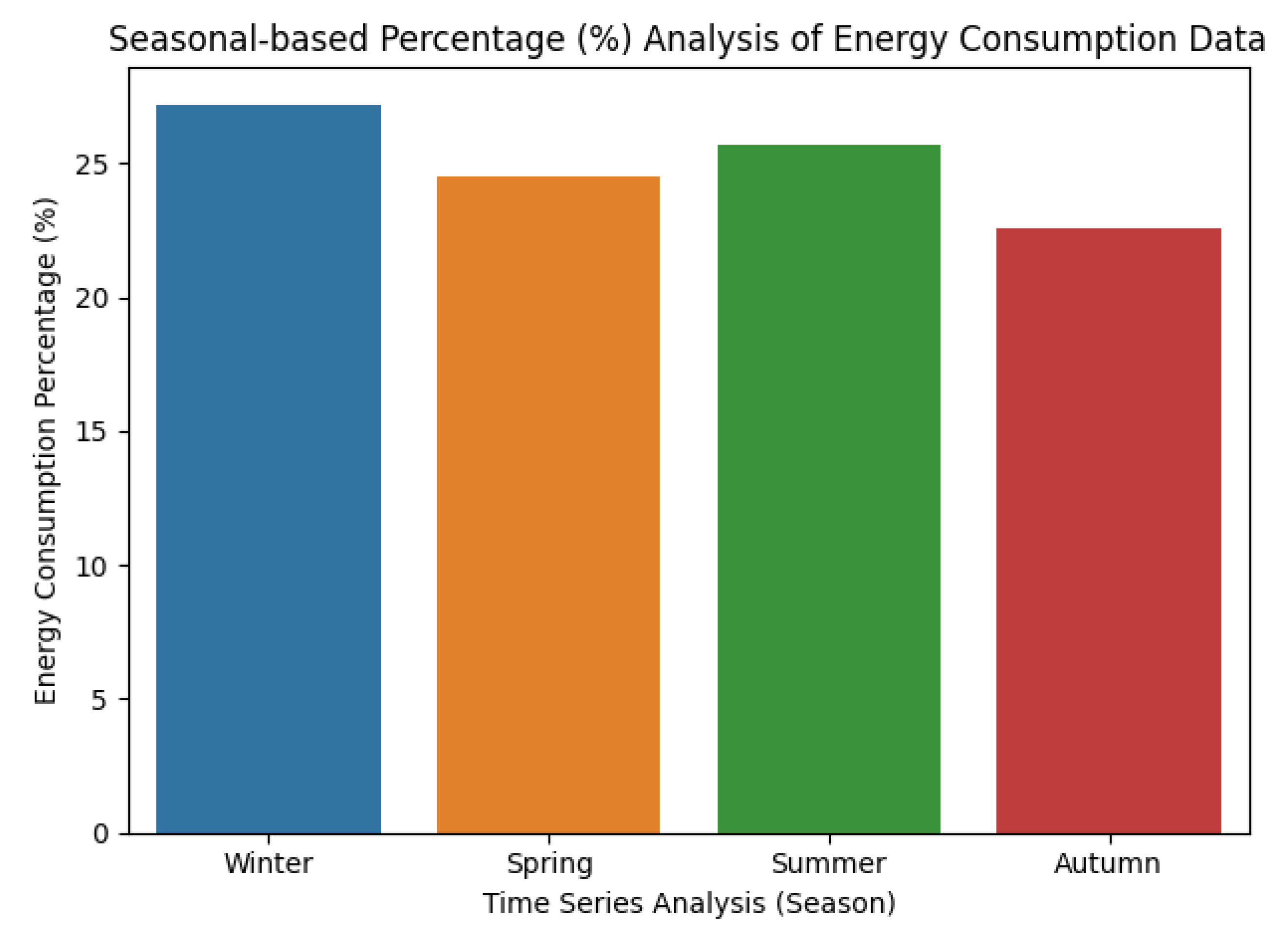
Figure 8 presents seasonal-based percentage analysis of the electric energy consumption. The impacts of seasonal variation can be seen in the corresponding electric consumption.
The consumption share of winters is the highest because South Korea has extremely cold winters; hence, heating appliances increase electricity consumption. Thus, occupants consume more electricity according to their comfort levels and special needs. Weather predominantly affects the consumption patterns and thus temperature has a highly negative correlation with electric consumption compared to humidity, hence seasonal variations also change consumption profiles. Therefore, a seasonal-based percentage analysis has been performed to get a clear insight into seasonal based percentage of consumption. Table 2 summarized seasonal-based percentage analysis of electric energy consumption. It is evident that Winter has the highest percentage as compared to the other seasons, such as Spring, Summer, and Autumn. It is also evident that Autumn is the low percentage of 22.60% as compared to other seasons.
This representation has been very effective in our analysis and understanding of the distribution of the data. The electric consumption data are sparse, yet a seasonal pattern is evident in the distribution, which motivated us to use it for the generalization of the sequence based LSTM-Kalman model.
4.4. Correlation Analysis
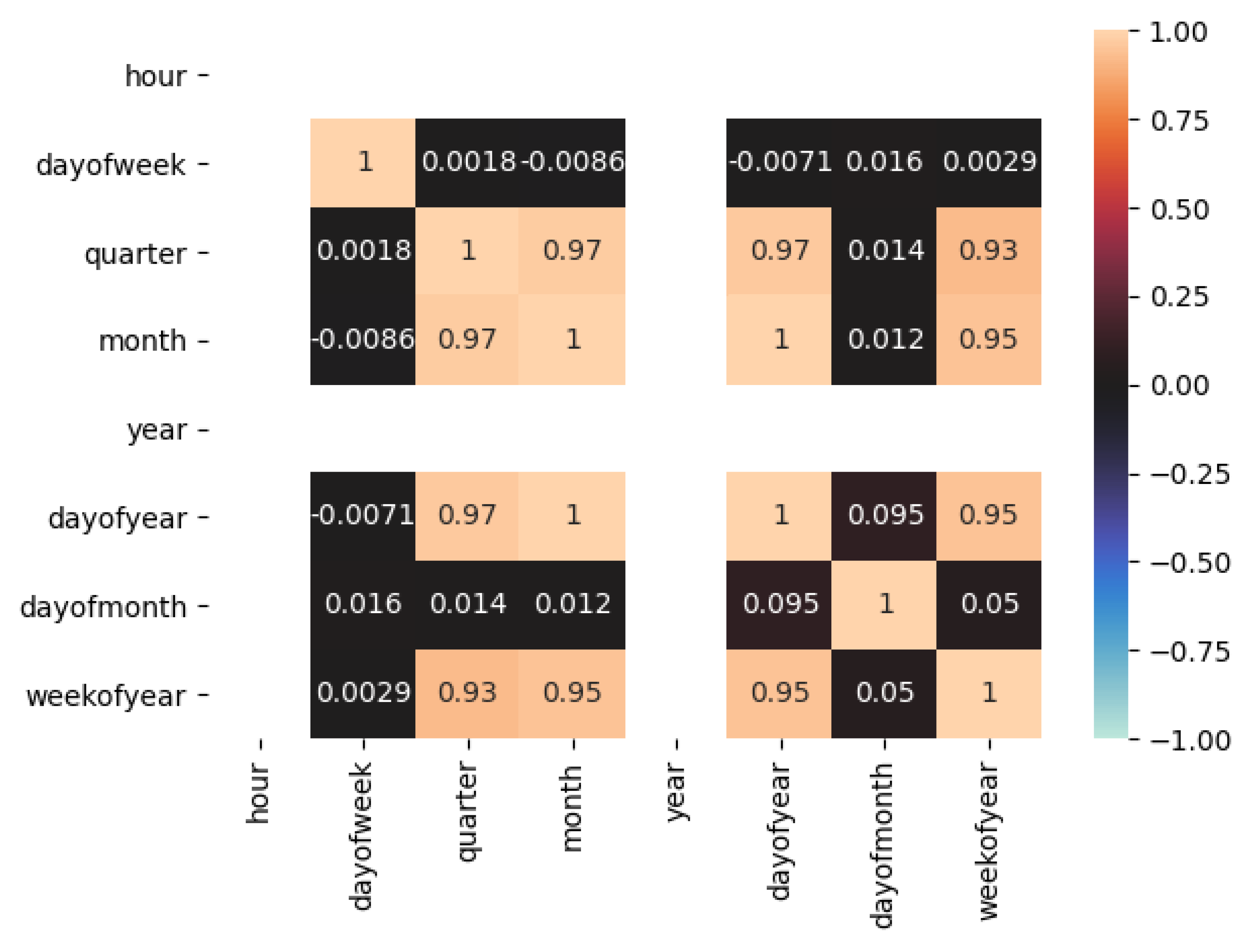
Correlation analysis lies under the category of statistical methods that measure the degree of relationship strength and associations between continuous variables (quantitative/continuous). Figure 9 presents the correlation analysis of then extracted time-series data based on hourly, days of week based, quarterly, monthly, yearly, days of year based, days of month based, and weeks of year based. The relationship between variables specify how well they relate to one another such that we can ascertain their future behavior and impact. Correlation analysis involves a correlation coefficient that assigns value to the relationship between variables. The relationship between variables can be negative, positive, and or no relationship at all. High correlation depicts a strong relationship while weak correlation value means variables are least related to each another. It is evident from the figure how electric consumption on particular days is correlated. It can be found that the day of year feature is contributed more compared to other proposed features. It is evident that the following features can be eliminated from the prediction process, such as hour, quarter, month, and year because of low contribution in the model training process.
5. Ensemble Prediction Approach for Efficient Building Energy Management
This section presents prediction models developed to forecast electric consumption of multi-family storied residential buildings. This paper employed three different models, such as Long Short Term Memory (LSTM), Kalman Filter, and ensemble prediction model by integrating LSTM and Kalman Filters to predict energy consumption requirements of the residential buildings for energy management.
5.1. LSTM Model
Recurrent neural network (RNN) is a special case of artificial neural network (ANN) designed for extracting hidden patterns from data sequences such as time series data, text and NLP, etc. RNN is based on time and the sequence of data during that time; as sequential data have temporal correlations, RNN is a powerful tool to deal with temporal dependencies. The specialty of RNN is the memory units, which make them perfect for dealing time series problems. RNN efficiently uses sequential information because each node is directly connecting to the successive nodes in a layer. Recurrent nets are named as recurrent because they have feedback looping structures to save information for future use. These memory units work recursively to calculate new cell states through application of activation functions on new inputs and old/previous cell states. Information in RNN circulates in hidden nodes, which helps to find correlations between different events called long term dependencies. Theoretically, RNN can utilize information contained in long sequences; practically, they have the ability to only look back a few steps.
To provide a solution to the problem of vanishing gradient, in order to allow deeper neural networks and recurrent neural nets to work together practically, we need a mechanism through which we can lessen the number of gradients’ multiplication that are less than zero. It works by using internal memory state, adding it to the (processed) input so that the multiplicative effect of smaller gradients is reduced significantly. LSTM possesses memory cells and gates such as input, forget, and output gate; these gates ensure the preserving of error that propagates back through layers and continue to learn over various time steps.
Figure 10 shows the simplified representation of LSTM; in the first step, the network decides if there is any information that is irrelevant in a particular time step and needs to be deleted from the cell. Sigmoid function is the one that makes this decision by considering the present input and the current state and then calculates the function. The gate involved in step one is known as the forget gate. Basically, it forgets the information that is not needed or the one that is less important. In the second step, the forget gate decides how much of this unit adds to the current state; this steps has two functions involved; the first one is a sigmoid function, and the second one is the Tanh (tangent hyperbolic function). The first function acts like a filter and decides which values to let in. The tangent hyperbolic function adds weights to these values. Weights are assigned to values on the basis of their importance in the current context. The gate involved in this step is called input gate. The input gate decides which information to let through based on its importance. The input gate adds some new information to the current input. In the last step, the output gate calculates the output, involving two layers. One is the sigmoid layer that makes a decision about which cell parts/states will be output. Then, the cell states values are passed to a tangent hyperbolic function to push them between (−1 +1) and then the answer is multiplied to a sigmoid gate output.
5.2. Kalman Filter
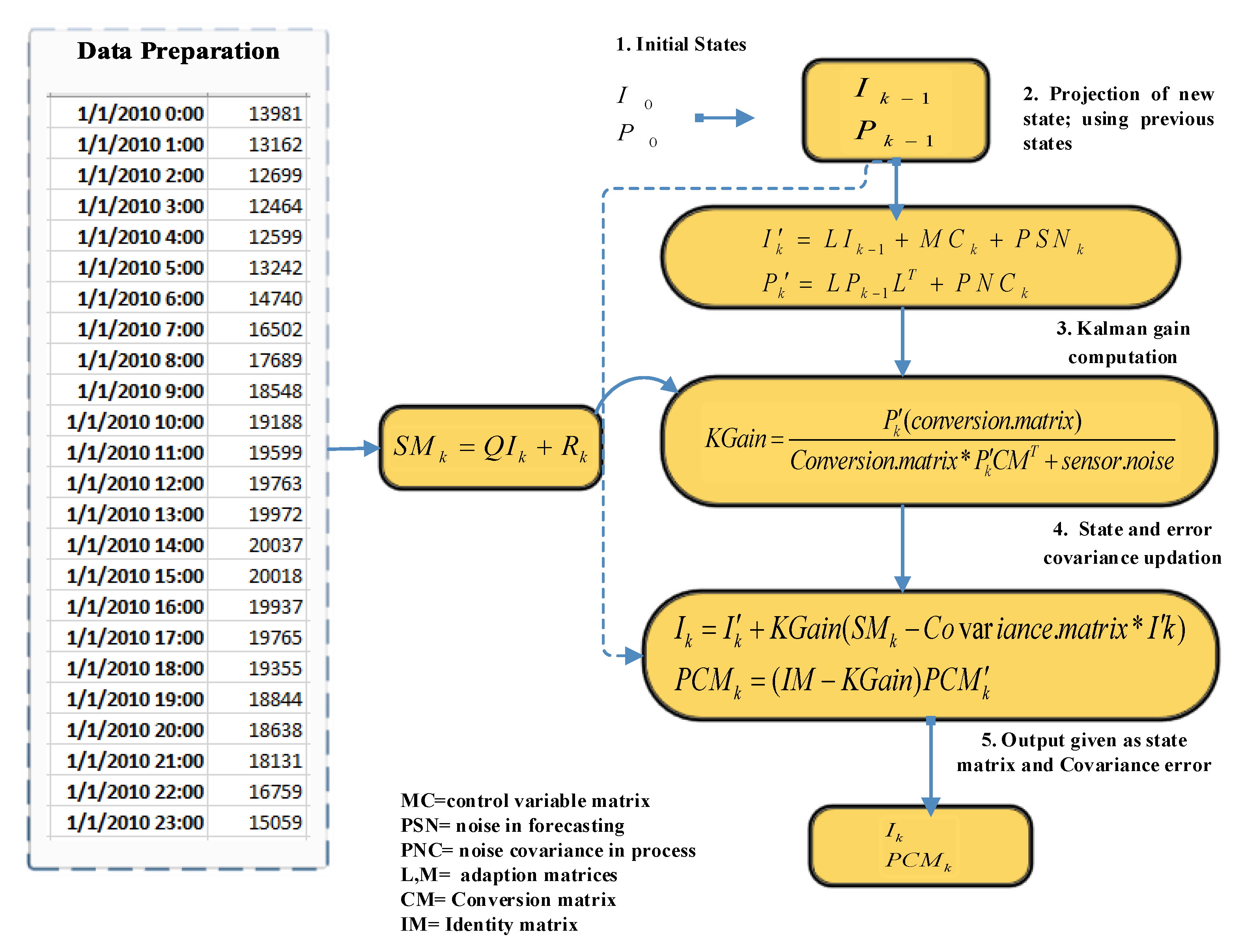
Kalman Filter (KF) is a stochastic algorithm that is used to estimate the dynamic system states through noisy readings, which make it a multi-functional algorithm both as a predictor and an estimator. During each time step, the network requires all information up to the present point including derivatives computed since learning began (from the first iteration). It provides estimation of current value based on previous estimate reading and the most recent reading. Figure 11 is used to represent the basic flow of the Kalman Filter. Basically, KF has two modules: one in prediction (state variable estimation) and the other is correction (state variables correction). KF can be modeled mathematically using the following equations [11].
The step-by-step formulation process of KF is shown to predict electricity consumption of multifamily residential buildings to facilitates policy-makers. The following Equation (2) is used to predict a new state based on the previous state:
The prediction of a new state is done on the basis of the previous state ( and ) and the output of a physical model with a correction term added in the prediction error in the form of predicted state noise and process noise covariance error so that error is minimized. represents a control variable matrix while is noise in prediction, i.e., (process state noise). The next step is calculated as defined in Equation (3):
where represents noise covariance levels (estimated error) in a particular process, L represents the state transaction matrix, and is used to indicate the transpose of the state transaction matrix. represents the last instance of the covariance factor. Using KM, we are able to calculate the likelihood function of error in prediction, which is further utilized for the system’s unknown (future consumption behavior) parameter estimation.
is calculated in phase two, called the correction of state variables phase using the measurements from an input, such as electric consumption state and noise level measurements. In this study, plays a significant role as it can significantly influence the performance of KF in controlling behavior. It is updated using iteration based on the conversion matrix and estimated error in the measurement process. The is defined as shown in Equation (4):
where represents conversion (observation) matrix, represents transpose of observation matrix, and R indicates the estimated error in the prediction process.
Kalman gain makes the decision of more weight assignment to any one of them: estimate or measurement. After Kalman gain computation, we update the states and covariance error using the following Equations (5) and (6). Let represent the recent consumption of energy at time t. Then, we can use Equation (5) to predict the actual energy consumption of multi-residential buildings to facilitate energy providers for effective policy-making:
and finally Equation (6) is used to update covariance factor for the next iteration (observation):
where represents state matrix and represents covariance error states as the output.
5.3. Proposed Ensemble Prediction Model
This subsection presents flow of the proposed ensemble prediction approach. Figure 12 presents basic flow of the proposed ensemble prediction model. The proposed ensemble approach is comprised of different steps, such as acquisition of electricity consumption data, preprocessing and normalization of data, training and testing ensemble model, and evaluation of the proposed model using different metrics. The first step for learning to prediction is data acquisition. The experiments have been performed on a real electric consumption dataset acquired from four multi-storied multifamily residential buildings situated in South Korea. Data preprocessing is a critical step that directly influences the model performance and results make data ready for model building; the first step is data preprocessing, so that optimal model performance can be achieved. Preprocessing data are a multi step process; each step has the same goal of building the best predictive model. For our model, we normalized our data by scaling it in a specified range as it is important to scale the data before model training so that the difference in attributes could be well adjusted. After data normalization, we split our data into training and test sets. Training set is further supplied to the LSTM model to learn the complex input to output mappings. While the test set is for model evaluation, actual case predictions from the training data model are acquired on the testing data set inputs and are kept for comparison with test set outputs so that performance can be evaluated. After training the model, the validation step comes. It is another way to evaluate the model on unseen data and ascertain how well the model behaves in an average case or how well the generalizability holds. After model validation error is calculated we tune the model hyper-parameters in such a way that error is minimized. Once the desired error threshold is attained, the learning process is stopped, and the resulting data are sent to the combinator where the results are combined with KF prediction results. The test data is also fed to the KF with the purpose of optimal parameter estimation of variables. It has the ability to predict the error covariance in the prediction process and state ahead by computing the Kalman gain. Basically, KF aids the process of acquiring reliable estimates based on observed sequential data. The estimated energy consumption output is sent to the combinator where it is combined with the LSTM output, and the aggregated mean is calculated. Lastly, the system outputs the final short-term electric energy prediction based on which the performance analysis is done using MAE, RMSE, MAPE, and R2 score.
6. Experimentation Environment, Results, and Performance Analysis
This section presents experimentation environment, short-term energy prediction results, and performance analysis.
6.1. Experimentation Environment
This subsection discusses the experimentation environment of the proposed ensemble prediction model based on the learning to statistical approach. The development of proposed models is done using Python programming language. Moreover, preprocessing of data and regression analysis is completed using a library called scikit learn. Pykalman and predict function in KF have been applied to attain electric consumption prediction. Table 3 presents the implementation setup of the proposed ensemble prediction model.
6.2. Short-Term Energy Consumption Demands’ Prediction Results
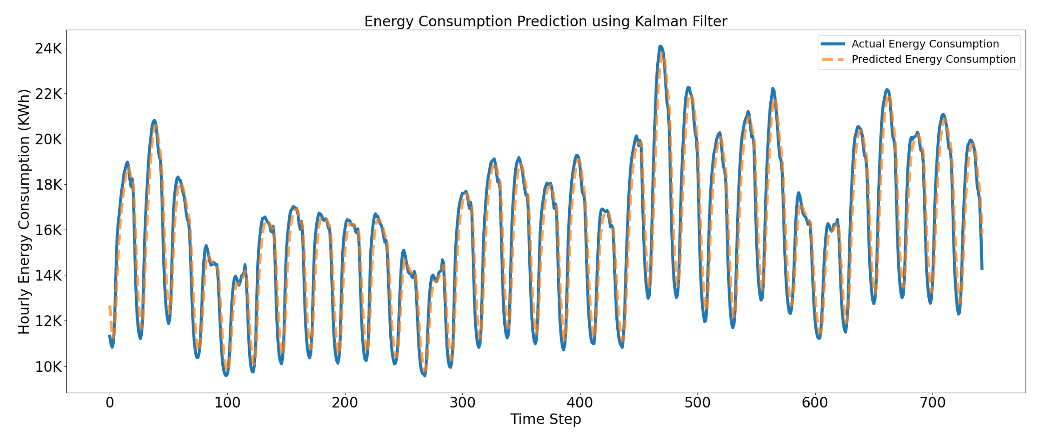
This subsection presents energy prediction results obtained using KF, LSTM, and the ensemble prediction model. KF is used as a stochastic model to forecast the hourly electric consumption and is expressed in terms of a linear function of inputs. It uses the past electric consumption data in order to estimate the parameters of the model. The experimental results presented in Figure 13 clearly depict that the independent Kalman model performs slightly worse than other solutions due to its dependency on the dynamic model. Moreover, due to diversity in human behavior, the electric consumption patterns in multistoried residential apartments are highly dissimilar; therefore, the trained model is behaving differently on the test set, and the error becomes high in that case.
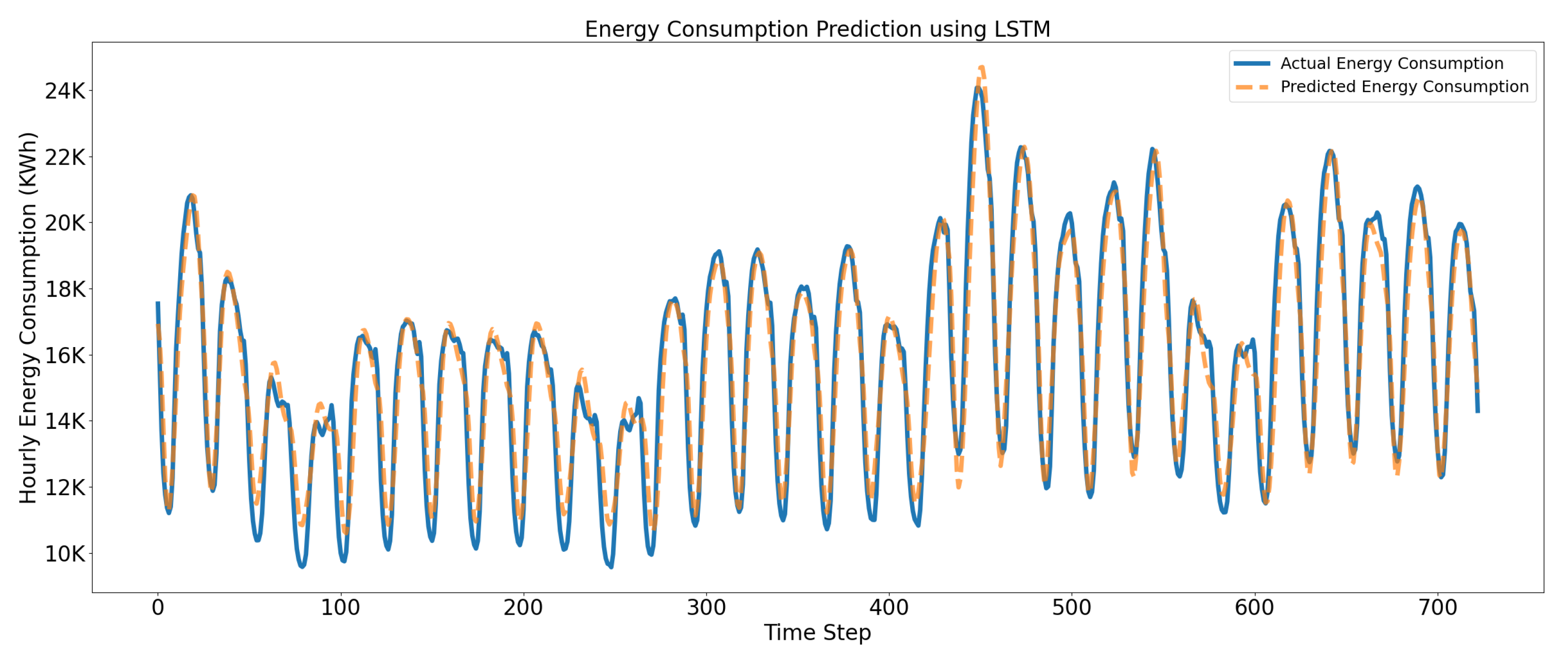
Figure 14 shows the daily prediction of the electricity consumption by LSTM. We can analyze from the results of statistical measures that performance of the independent LSTM model is better than the independent Kalman model. It is evident that the LSTM model performed well and provided accurate electric consumption prediction as compared to the Kalman Filter. The overall performance of the LSTM prediction model in terms of MAE, RMSE, MAPE, and R2 score is 557.96, 695.552, 3.925, and 0.956, respectively. The core reason for LSTM to outperform the Kalman-filter prediction model is due to its ability to learn the sequential behavior of the electric consumption; moreover, they are more efficient at the learning context for predicting electricity consumption.
Similarly, Figure 15 presents the comparative analysis of the actual and predicted electric consumption yield by the ensemble prediction model based on the learning to statistical approach (combined using Mean). It is evident from the results that there is a significant improvement in prediction performance, and the model has produced more stable results (MAPE and R2 scores) compared to independent models. The performance of the model is attributed to the dynamic adjustment capability of the Kalman Filter. The prediction performance of the ensemble prediction model in terms of MAE, RMSE, MAPE, and R2 score is 373.58, 487.0, 3.264, and 0.966, respectively. Hence, the ensemble prediction model provides a better fit and generalization to data and also increases the overall performance of the prediction model in terms of R2 score as compared to independent KF and LSTM models.
Lastly, Figure 16 presents an overall comparative analysis of the proposed hourly energy consumption prediction models. The following Figure 16 presents a comparative analysis of actual and predicted consumption of the electricity produced by the ensemble prediction model, independent Kalman Filter, and independent LSTM.
It can be observed from the values of statistical measures that the ensemble model performs far better as compared to counterpart independent prediction models. Experimental results prove that the proposed ensemble prediction approach yields better hourly consumption prediction results because of the integration of the learning module, as it continuously monitors and improves the outcome of the prediction module by tuning the Kalman gain (R) parameter; furthermore, it also proved that the ensemble LSTM-Kalman model is more robust and can yield superior performance by reducing over-fitting, while controlling and minimizing the variance of prediction errors caused by the individual contributing prediction models.
6.3. Feature Importance
For analysis of features and their impact on the output of the prediction model, we attempted to efficiently portray the features and their corresponding scores based on their usefulness and impact on the target variable. Feature importance analysis plays a vital part in the provisioning of data insights, which further facilitates the data analytics’ process flow such as dimensionality reduction and feature selection so that an improved predictive model can be built. Feature analysis can help understand data and the model in a more appropriate way, enhancing the feature selection process such that the number of features that are least important are not considered. Figure 17 presents feature importance analysis using conventional ensemble models.
In the following Figure 17a, RF based feature importance shows that the day of the year feature is the most important among all the features. While the second highest score is achieved by the day of the week feature. Figure 17b depicts the proposed feature importance based on XGBoost; it is evident that the week of the year feature has attained the highest score and is hence the most impactful feature on the target variable compared to the other features. While the quarter features have the lowest score and the least importance among the rest of them. Proposed feature importance based on Adaboost depicts that week of the year and day of the year are highly important features while day of week holds the third position based on feature importance score. The GB based feature has similar results compared to XGBoost features, the week of the year has achieved the highest scores, the day of the year features achieved the second highest score, and the day of the week has maintained the third position as in case of XGBoost-features. Overall, the week of the year was found to be the most influential feature among all eight features.
6.4. Performance Evaluation
This subsection presents an overview of various performance measures employed in the proposed work; these include MSE, RMSE, MAPE, and R2 score, to evaluate the performance of the implemented prediction models. Accuracy of electricity consumption prediction can be determined using various measures. A low error value means more accurate predictions. Hence, accuracy measures the difference between actual output and predicted output. Generally, testing and comparing various prediction models and approaches, using a similar dataset, every accuracy measure will produce different results and hence different performance. To compare the results with other techniques, mean absolute error (MAE), mean absolute percentage error (MAPE), R2 score, and root mean square error (RMSE) are the selected pewrformance evaluation metric used for performance evaluation of models [55,56].
The scale dependent measure we applied to evaluate our model is MAE and RMSE:
Root mean square error (RMSE) is also a scale dependent accuracy measure; we applied it depending on squared error:
Percentage dependent accuracy measures employ the percentage concept, where 100 is multiplied with prediction error/actual output observation at the time; this measure of accuracy is scale independent and measures the prediction values independent of the data set used; hence, we can compare the performance of different methods using this. This accuracy measure is the most useful and widely used accuracy measure. MAPE is based on absolute percentage error calculated for each time period. The actual output minus the predicted value divided by the actual values give the answer. The formula for MAPE calculation is as follows:
Another evaluation index used by this study is the determination coefficient which measures the capacity of model to forecast new data similar to the mean square error; it also shows how well the model fits to data:
Figure 18 presents comparative analysis of the implemented prediction models in terms of MAPE and R2 score. It depicts that our ensemble prediction model has achieved the highest R2 score of 0.966. The prediction error of the proposed approach is small compared to other models. It is also evident that the performance of ensemble electric consumption prediction model is up to the mark due to its ability to map temporal correlations and handle long-term dependencies. Hence, our proposed ensemble prediction approach outperformed all other implemented models and produced relatively better prediction results because the proposed ensemble prediction model is capable of managing the bias-variance trade-off so that error could be minimized.
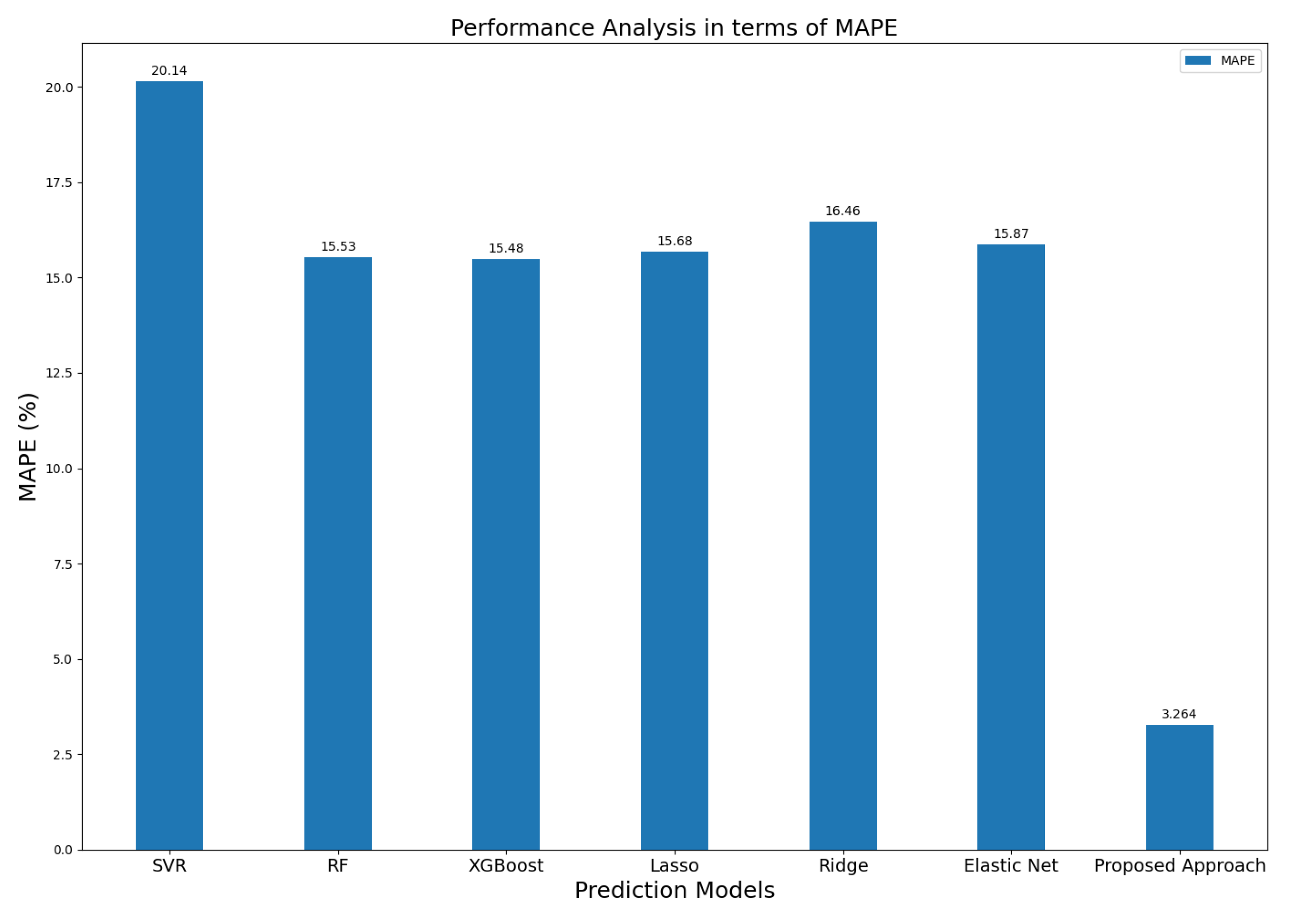
Similarly, Figure 19 shows a comparison between the proposed approach with traditional ML models. It is evident from the MAPE scores that the proposed ensemble electric consumption prediction model performed best comparative to traditional machine learning prediction models. The proposed ensemble prediction approach achieved the highest accuracy and lowest MAPE, which further supports the effectiveness of the proposed work in the domain of electric consumption prediction. The proposed ensemble model achieved a low error in the prediction process compared to the traditional ML models. As evident from the figure, the lowest MAPE achieved by our proposed work is attributed to the choice of LSTM as a learner providing better generalization, controllability, and results along with KF as an optimal solution by capturing temporal dependencies.
Table 4 shows accuracy of hourly predictions; the results illustrate that the ensemble prediction approach outperforms the rest of the solutions. The prediction performance of the ensemble prediction approach in terms of MAPE and R2 score is 3.264 and 0.966, respectively. Due to diversity in human behavior, external weather conditions, and several other influencing factors, the electric consumption patterns in multi-storied residential apartments are highly dissimilar; therefore, the trained model behaved differently on the test set and the probability of prediction error becomes high in this case. Our proposed ensemble approach has produced more stable results as compared to proposed independent prediction models based solution approaches. LSTM also achieved satisfactory results with the lowest MAPE of 4.64 for hourly predictions because load profiling provisions additional information to the model and significantly. In simpler terms, we can say that the electric consumption of a particular hour on a particular day depends upon the consumption of all the previous hours and days in a series. As there is information contained in every sequence itself, considering information contained in each sequence is imperative for achieving optimal prediction performance of the model.
Table 5 shows performance evaluation results of the proposed electricity consumption prediction model and conventional ensemble models. This study compared the proposed prediction model with conventional ensemble models to highlight the significance of the proposed work. The performance of the proposed LSTM-Kalman model is significantly better comparative to the traditional ensemble models. The conventional XGBoost model performed relatively accurately to the AdaBoost and gradient boosting (GB). The R2 score analysis shows that the proposed prediction model accurately predicts short-term energy loads compared to the conventional ensemble models, such as XGBoost, AdaBoost, and GB. Hence, our proposed energy prediction model outperformed the conventional ensemble models.
Furthermore, the results produced by our ensemble prediction model are compared and evaluated with traditional ML-based algorithms as shown in Table 6. The comparative analysis shows that our proposed model has achieved superior performance in terms of MAPE comparative to classic machine Learning models. The proposed ensemble approach acquired the lowest MAPE of 3.264, which proves the strength of our ensemble electricity consumption prediction model for short-term electric consumption forecasting. The performance of other well established ML models, such as Lasso (L1), Ridge (L2), Elastic Net, and XGBoost is comparatively low in terms of MAPE, while the performance of Support Vector Regressor (SVR) in terms of MAPE is not up to the standard compared to conventional ML models. Hence, comparative analysis in terms of MAPE makes it obvious that our proposed ensemble approach produced promising results compared to the conventional ML algorithms.
7. Conclusions
Electrcity consumption prediction model assist policymakers with assessing the impact of future electric consumption and demand and formulate current and future policies based on that. This paper presented data and predictive analytics modules to forecast short term electricity consumption based on a time-series dataset acquired from multifamily residential buildings, South Korea. First, the time-series based analysis module is presented to highlight hidden insights and characteristics of the energy consumption data to manage and control energy supply and demands. Second, an ensemble prediction approach is proposed to integrate LSTM and KF using an aggregated mean based on a real dataset of electricity consumption acquired from multifamily residential buildings. The main contribution of our proposed work is to integrate deep learning and a statistical model for short-term electricity consumption prediction of multifamily residential buildings. Furthermore, it aims to facilitate stakeholders to devise effective policies for managing energy supply and demands to mitigate power outages and blackouts; moreover, it ensures prevention of resource wastage. Furthermore, the following performance measures are used to evaluate the overall prediction performance, such as MAE, RMSE, MAPE, and R2 score. The comparative analysis illustrates that the proposed ensemble electric consumption prediction model outperformed counterpart models for short-term energy forecasting. The comparative results justified the hypothesis made in this study that the sequence-based model, if integrated with a statistical model like the Kalman Filter, yields better generalization than the non-sequential models.
A future direction would be applying this technique to various other datasets, through advance feature selection processes, improved data analytic techniques, improving the input features (weather and holidays features), and applying some feature selection process to achieve more accuracy. Furthermore, we will extend this work to forecast daily, weekly, and monthly energy consumption at apartment, floor, and residential building levels. Moreover, we will extend our work to develop a city-wise model over different geographical areas.
Author Contributions
Conceptualization, A.N.K., N.I. and D.-H.K.; Methodology, A.N.K. and D.-H.K.; Software, A.N.K. and N.I.; Validation, N.I., R.A. and D.-H.K.; Formal Analysis, A.N.K. and N.I.; investigation, A.N.K.; Data Curation, A.N.K. and R.A.; writing—original draft preparation, A.N.K. and N.I.; writing—review and editing, R.A. and N.I.; Visualization, N.I. and R.A.; Supervision, D.-H.K.; Project Administration, D.-H.K.; Funding Acquisition, D.-H.K. All authors have read and agreed to the published version of the manuscript.
Funding
This research was supported by Energy Cloud R&D Program through the National Research Foundation of Korea (NRF) funded by the Ministry of Science, ICT (2019M3F2A1073387), and this research was supported by Institute for Information & communications Technology Planning & Evaluation (IITP) grant funded by the Korea government (MSIT) (No.2018-0-01456, AutoMaTa: Autonomous Management framework based on artificial intelligent Technology for adaptive and disposable IoT). Any correspondence related to this paper should be addressed to Dohyeun Kim.
Conflicts of Interest
The authors declare no conflict of interest regarding the publication of this paper.
References
- Ahmad, M.W.; Mourshed, M.; Rezgui, Y. Trees vs. Neurons: Comparison between random forest and ANN for high-resolution prediction of building energy consumption. Energy Build. 2017, 147, 77–89. [Google Scholar] [CrossRef]
- Connolly, R.; Connolly, M.; Carter, R.M.; Soon, W. How Much Human-Caused Global Warming Should We Expect with Business-As-Usual (BAU) Climate Policies? A Semi-Empirical Assessment. Energies 2020, 13, 1365. [Google Scholar] [CrossRef] [Green Version]
- Penya, Y.K.; Borges, C.E.; Fernández, I. Short-term load forecasting in non-residential buildings. In Proceedings of the IEEE Africon’11, Victoria Falls, Zambia, 13–15 September 2011; pp. 1–6. [Google Scholar]
- Deb, C.; Zhang, F.; Yang, J.; Lee, S.E.; Shah, K.W. A review on time series forecasting techniques for building energy consumption. Renew. Sustain. Energy Rev. 2017, 74, 902–924. [Google Scholar] [CrossRef]
- Khan, P.W.; Byun, Y.C.; Lee, S.J.; Park, N. Machine Learning Based Hybrid System for Imputation and Efficient Energy Demand Forecasting. Energies 2020, 13, 2681. [Google Scholar] [CrossRef]
- Alvarez, F.M.; Troncoso, A.; Riquelme, J.C.; Ruiz, J.S.A. Energy time series forecasting based on pattern sequence similarity. IEEE Trans. Knowl. Data Eng. 2010, 23, 1230–1243. [Google Scholar] [CrossRef]
- Iqbal, N.; Jamil, F.; Ahmad, S.; Kim, D. Toward Effective Planning and Management Using Predictive Analytics Based on Rental Book Data of Academic Libraries. IEEE Access 2020, 8, 81978–81996. [Google Scholar] [CrossRef]
- Singh, S.; Yassine, A. Big data mining of energy time series for behavioral analytics and energy consumption forecasting. Energies 2018, 11, 452. [Google Scholar] [CrossRef] [Green Version]
- Gridach, M. Character-level neural network for biomedical named entity recognition. J. Biomed. Inform. 2017, 70, 85–91. [Google Scholar] [CrossRef]
- Ahmad, N.; Han, L.; Iqbal, K.; Ahmad, R.; Abid, M.A.; Iqbal, N. SARM: Salah activities recognition model based on smartphone. Electronics 2019, 8, 881. [Google Scholar] [CrossRef] [Green Version]
- Jamil, F.; Iqbal, N.; Ahmad, S.; Kim, D.H. Toward accurate position estimation using learning to prediction algorithm in indoor navigation. Sensors 2020, 20, 4410. [Google Scholar] [CrossRef] [PubMed]
- Ahmad, S.; Iqbal, N.; Jamil, F.; Kim, D. Optimal Policy-Making for Municipal Waste Management Based on Predictive Model Optimization. IEEE Access 2020, 8, 218458–218469. [Google Scholar] [CrossRef]
- Sutskever, I.; Vinyals, O.; Le, Q.V. Sequence to sequence learning with neural networks. Adv. Neural Inf. Process. Syst. 2014, 27, 3104–3112. [Google Scholar]
- Bengio, Y.; Courville, A.; Vincent, P. Representation learning: A review and new perspectives. IEEE Trans. Pattern Anal. Mach. Intell. 2013, 35, 1798–1828. [Google Scholar] [CrossRef]
- Rahman, A.; Srikumar, V.; Smith, A.D. Predicting electricity consumption for commercial and residential buildings using deep recurrent neural networks. Appl. Energy 2018, 212, 372–385. [Google Scholar] [CrossRef]
- Kong, W.; Dong, Z.Y.; Jia, Y.; Hill, D.J.; Xu, Y.; Zhang, Y. Short-term residential load forecasting based on LSTM recurrent neural network. IEEE Trans. Smart Grid 2017, 10, 841–851. [Google Scholar] [CrossRef]
- Ullah, I.; Fayaz, M.; Kim, D. Improving accuracy of the kalman filter algorithm in dynamic conditions using ANN-based learning module. Symmetry 2019, 11, 94. [Google Scholar] [CrossRef] [Green Version]
- Ecotect. Available online: https://web.archive.org/web/20080724093511/http://squ1.com/products/ecotect/ (accessed on 20 December 2020).
- Energy Plus. Available online: https://energyplus.net/ (accessed on 20 December 2020).
- DOE2. Available online: https://www.doe2.com/ (accessed on 20 December 2020).
- Integrated Environmental Solutions (IES). Available online: https://www.iesve.com/ (accessed on 20 December 2020).
- Esen, H.; Esen, M.; Ozsolak, O. Modelling and experimental performance analysis of solar-assisted ground source heat pump system. J. Exp. Theor. Artif. Intell. 2017, 29, 1–17. [Google Scholar] [CrossRef]
- Bourdeau, M.; Zhai, X.Q.; Nefzaoui, E.; Guo, X.; Chatellier, P. Modeling and forecasting building energy consumption: A review of data-driven techniques. Sustain. Cities Soc. 2019, 48, 101533. [Google Scholar] [CrossRef]
- Christiaanse, W. Short-term load forecasting using general exponential smoothing. IEEE Trans. Power Appar. Syst. 1971, 2, 900–911. [Google Scholar] [CrossRef]
- Pappas, S.S.; Ekonomou, L.; Karamousantas, D.C.; Chatzarakis, G.; Katsikas, S.; Liatsis, P. Electricity demand loads modeling using AutoRegressive Moving Average (ARMA) models. Energy 2008, 33, 1353–1360. [Google Scholar] [CrossRef]
- Papalexopoulos, A.D.; Hesterberg, T.C. A regression-based approach to short-term system load forecasting. IEEE Trans. Power Syst. 1990, 5, 1535–1547. [Google Scholar] [CrossRef]
- Amjady, N. Short-term hourly load forecasting using time-series modeling with peak load estimation capability. IEEE Trans. Power Syst. 2001, 16, 498–505. [Google Scholar] [CrossRef]
- Chae, Y.T.; Horesh, R.; Hwang, Y.; Lee, Y.M. Artificial neural network model for forecasting sub-hourly electricity usage in commercial buildings. Energy Build. 2016, 111, 184–194. [Google Scholar] [CrossRef]
- Quilumba, F.L.; Lee, W.J.; Huang, H.; Wang, D.Y.; Szabados, R.L. Using smart meter data to improve the accuracy of intraday load forecasting considering customer behavior similarities. IEEE Trans. Smart Grid 2014, 6, 911–918. [Google Scholar] [CrossRef]
- Dong, B.; Li, Z.; Rahman, S.M.; Vega, R. A hybrid model approach for forecasting future residential electricity consumption. Energy Build. 2016, 117, 341–351. [Google Scholar] [CrossRef]
- Paudel, S.; Elmitri, M.; Couturier, S.; Nguyen, P.H.; Kamphuis, R.; Lacarrière, B.; Le Corre, O. A relevant data selection method for energy consumption prediction of low energy building based on support vector machine. Energy Build. 2017, 138, 240–256. [Google Scholar] [CrossRef]
- Jozi, A.; Pinto, T.; Praça, I.; Ramos, S.; Vale, Z.; Goujon, B.; Petrisor, T. Energy consumption forecasting using neuro-fuzzy inference systems: Thales TRT building case study. In Proceedings of the 2017 IEEE Symposium Series on Computational Intelligence (SSCI), Honolulu, HI, USA, 27 November–1 December 2017; pp. 1–5. [Google Scholar]
- Bagis, A. Fuzzy rule base design using tabu search algorithm for nonlinear system modeling. ISA Trans. 2008, 47, 32–44. [Google Scholar] [CrossRef]
- Hinton, G.E.; Osindero, S.; Teh, Y.W. A fast learning algorithm for deep belief nets. Neural Comput. 2006, 18, 1527–1554. [Google Scholar] [CrossRef]
- Hochreiter, S.; Schmidhuber, J. Long short-term memory. Neural Comput. 1997, 9, 1735–1780. [Google Scholar] [CrossRef] [PubMed]
- Urban, G.; Geras, K.J.; Kahou, S.E.; Aslan, O.; Wang, S.; Caruana, R.; Mohamed, A.; Philipose, M.; Richardson, M. Do deep convolutional nets really need to be deep and convolutional? arXiv 2016, arXiv:1603.05691. [Google Scholar]
- Dedinec, A.; Filiposka, S.; Dedinec, A.; Kocarev, L. Deep belief network based electricity load forecasting: An analysis of Macedonian case. Energy 2016, 115, 1688–1700. [Google Scholar] [CrossRef]
- Mocanu, E.; Nguyen, P.H.; Gibescu, M.; Kling, W.L. Deep learning for estimating building energy consumption. Sustain. Energy Grids Netw. 2016, 6, 91–99. [Google Scholar] [CrossRef]
- El-Sharkh, M.Y.; Rahman, M.A. Forecasting electricity demand using dynamic artificial neural network model. In Proceedings of the 2012 International Conference on Industrial Engineering and Operations Management, Istanbul, Turkey, 3–6 July 2012; pp. 3–6. [Google Scholar]
- Qiu, X.; Zhang, L.; Ren, Y.; Suganthan, P.N.; Amaratunga, G. Ensemble deep learning for regression and time series forecasting. In Proceedings of the 2014 IEEE Symposium on Computational Intelligence in Ensemble Learning (CIEL), Singapore, 9–12 December 2014; pp. 1–6. [Google Scholar]
- Li, P.; Li, Y.; Xiong, Q.; Chai, Y.; Zhang, Y. Application of a hybrid quantized Elman neural network in short-term load forecasting. Int. J. Electr. Power Energy Syst. 2014, 55, 749–759. [Google Scholar] [CrossRef]
- Ertugrul, Ö.F. Forecasting electricity load by a novel recurrent extreme learning machines approach. Int. J. Electr. Power Energy Syst. 2016, 78, 429–435. [Google Scholar] [CrossRef]
- Mandal, P.; Senjyu, T.; Urasaki, N.; Funabashi, T. A neural network based several-hour-ahead electric load forecasting using similar days approach. Int. J. Electr. Power Energy Syst. 2006, 28, 367–373. [Google Scholar] [CrossRef]
- Marino, D.L.; Amarasinghe, K.; Manic, M. Building energy load forecasting using deep neural networks. In Proceedings of the IECON 2016-42nd Annual Conference of the IEEE Industrial Electronics Society, Florence, Italy, 24–27 October 2016; pp. 7046–7051. [Google Scholar]
- Tian, C.; Ma, J.; Zhang, C.; Zhan, P. A deep neural network model for short-term load forecast based on long short-term memory network and convolutional neural network. Energies 2018, 11, 3493. [Google Scholar] [CrossRef] [Green Version]
- Singh, P.; Dwivedi, P. Integration of new evolutionary approach with artificial neural network for solving short term load forecast problem. Appl. Energy 2018, 217, 537–549. [Google Scholar] [CrossRef]
- Nowotarski, J.; Liu, B.; Weron, R.; Hong, T. Improving short term load forecast accuracy via combining sister forecasts. Energy 2016, 98, 40–49. [Google Scholar] [CrossRef]
- Jamil, F.; Iqbal, N.; Imran; Ahmad, S.; Kim, D. Peer-to-Peer Energy Trading Mechanism based on Blockchain and Machine Learning for Sustainable Electrical Power Supply in Smart Grid. IEEE Access 2021. [Google Scholar] [CrossRef]
- Al-Hamadi, H.; Soliman, S. Fuzzy short-term electric load forecasting using Kalman filter. IEE Proc. Gener. Transm. Distrib. 2006, 153, 217–227. [Google Scholar] [CrossRef]
- Stavrakakis, S.A.M.G.S.; Nikolaou, T.G. Short-term load forecasting based on the Kalman filter and the neural-fuzzy network (ANFIS). In Proceedings of the 2006 IASME/WSEAS International Conference on Energy & Environmental Systems, GREECE, Canary Islands, Spain, 16–18 December 2006; Volume 1, pp. 189–193. [Google Scholar]
- Jung, H.W.; Song, K.B.; Park, J.D.; Park, R.J. Very short-term electric load forecasting for real-time power system operation. J. Electr. Eng. Technol. 2018, 13, 1419–1424. [Google Scholar]
- Takeda, H.; Tamura, Y.; Sato, S. Using the ensemble Kalman filter for electricity load forecasting and analysis. Energy 2016, 104, 184–198. [Google Scholar] [CrossRef]
- Hu, Z.; Ma, J.; Yang, L.; Yao, L.; Pang, M. Monthly electricity demand forecasting using empirical mode decomposition-based state space model. Energy Environ. 2019, 30, 1236–1254. [Google Scholar] [CrossRef]
- Chujai, P.; Kerdprasop, N.; Kerdprasop, K. Time series analysis of household electric consumption with ARIMA and ARMA models. In Proceedings of the International MultiConference of Engineers and Computer Scientists, Hong Kong, China, 13–15 March 2013; Volume 1, pp. 295–300. [Google Scholar]
- Steyerberg, E.W.; Harrell, F.E., Jr.; Borsboom, G.J.; Eijkemans, M.; Vergouwe, Y.; Habbema, J.D.F. Internal validation of predictive models: Efficiency of some procedures for logistic regression analysis. J. Clin. Epidemiol. 2001, 54, 774–781. [Google Scholar] [CrossRef]
- Iqbal, N.; Jamil, F.; Ahmad, S.; Kim, D. A Novel Blockchain-based Integrity and Reliable Veterinary Clinic Information Management System using Predictive Analytics for Provisioning of Quality Health Services. IEEE Access 2021, 9, 8069–8098. [Google Scholar] [CrossRef]
Figure 1.
Basic flow of the proposed ensemble prediction model.

Figure 2.
Proposed ensemble prediction model architecture.

Figure 3.
Hourly electric energy consumption data (January 2010–January 2011).

Figure 4.
Daily electric energy consumption data (January 2010–December 2010).

Figure 5.
Weekly electric energy consumption data (January 2010–January 2011).

Figure 6.
Monthly percentage analysis of electric energy consumption (January 2010–January 2011).

Figure 7.
Energy consumption trends based on time-series analysis.

Figure 8.
Seasonal-based percentage analysis of electric energy consumption (January 2010–January 2011).
Figure 8.
Seasonal-based percentage analysis of electric energy consumption (January 2010–January 2011).

Figure 9.
Correlation analysis of the extracted time-series features.

Figure 10.
Simplified representation of LSTM.

Figure 11.
Basic flow of KF.

Figure 12.
Basic flow of the proposed ensemble prediction approach.

Figure 13.
Comparative analysis of actual and predicted hourly energy consumption requirements using KF.
Figure 13.
Comparative analysis of actual and predicted hourly energy consumption requirements using KF.

Figure 14.
Comparative analysis of actual and predicted hourly energy consumption requirements using LSTM.
Figure 14.
Comparative analysis of actual and predicted hourly energy consumption requirements using LSTM.

Figure 15.
Comparative analysis of actual and predicted hourly energy consumption requirements using the proposed ensemble prediction model.
Figure 15.
Comparative analysis of actual and predicted hourly energy consumption requirements using the proposed ensemble prediction model.

Figure 16.
Comparative analysis of proposed hourly energy consumption prediction models.

Figure 17.
Features’ importance analysis using conventional ensemble models.

Figure 18.
Performance evaluation in terms of MAPE and R2 Score.

Figure 19.
MAPE-based comparison of the proposed ensemble approach and traditional ML energy prediction models.
Figure 19.
MAPE-based comparison of the proposed ensemble approach and traditional ML energy prediction models.


Table 1.
Summary of the existing energy forecasting models.
| Model | Dataset | Types of Prediciton | MAPE (%) | Objective |
|---|---|---|---|---|
| Ensemble [1] | Weather and Time-Series Data | Heating and cooling energy consumption (Non-Residential) | 4.97 | Ensemble model to deal with multi-dimensional complex data |
| AR [3] | Weather and Time-Series Data | Overall energy consumption (Non-Residential) | 6.10 | Forecast energy hourly load of non-residential buildings using ARIMA and NN |
| Hybrid [30] | Energy consumption and building details | Overall energy consumption (Residential Single Family) | 5.30 | Integrated data-driven method with a physical model to forecast hourly and daily energy consumption |
| ANN [28] | Weather, Time-Series, and Operational | Commercial buildings energy prediction | 9.09 | Developed ANN-based energy forecasting model to predict short-term energy consumption |
| DBN [37] | Time-Series | Electric power systems of Macedonian | 8.6 | Developed DBN model to predict short-term electricity load and analyzed electricity consumptions of Macedonia city to extract hidden insights |
| FCRMB [38] | Time-Series | Energy Demand Consumption (Multifamily Residential) | 8.60 | Stochastic models were developed to analyze time-series data of energy consumption to forecast short-term energy load |
| HQENN [41] | Weather and Time-Series | Predict electricity load | – | Evolutionary technique is used to develop robust ANN model to forecast short-term energy load |
| RELM [42] | Time Series electric consumption data | Electric load forecasting | Developed RLEM model to forecast energy consumption load to facilitate energy providers | |
| S2S LSTM architecture [44] | Historical electric consumption data | Short term load forecasting | – | Deep learning based approach was proposed to predict power load to facilitate policymakers. |
| ANN-FTL [46] | Historical load and weather data | Short term load forecasting for load commercial market | 3.30 | Evolutionary algorithm was used to predict power load to help power distribution organizations |
Table 2.
Season-based percentage analysis of residential building energy consumption.
| Season | Percentage (%) |
|---|---|
| Winter | 27.20 |
| Spring | 24.50 |
| Summer | 25.70 |
| Autumn | 22.60 |
Table 3.
Experimentation setup of the proposed ensemble model.
| System Components | Description |
|---|---|
| Operating System | Microsoft Windows 10 (64-bits) |
| CPU | Intel® Core™ i5-4300 CPU at 3.40 GHz |
| RAM | 16 GB |
| Programming Language | Python |
| Storage | MySQL and MS Excel |
| IDE | PyCharm Professional |
Table 4.
Performance evaluation of energy prediction models.
| Model | MAE | RMSE | MAPE | R2 Score |
|---|---|---|---|---|
| Kalman Filter | 740.790 | 928.770 | 5.000 | 0.922 |
| LSTM | 557.960 | 695.552 | 3.925 | 0.956 |
| Proposed Model | 373.580 | 487 | 3.264 | 0.966 |
Table 5.
Performance evaluation and comparison of proposed ensemble approach with conventional ensemble prediction models.
Table 5.
Performance evaluation and comparison of proposed ensemble approach with conventional ensemble prediction models.
| Model | MAE | RMSE | MAPE | R2 Score |
|---|---|---|---|---|
| RF | 2095.669 | 2624.76 | 15.54 | 0.089 |
| XGBoost | 2083.946 | 2623.99 | 15.48 | 0.090 |
| AdaBoost | 2038.337 | 2683.314 | 15.80 | 0.048 |
| GB | 2039.429 | 2640.467 | 15.50 | 0.079 |
| Proposed Model | 373.580 | 487 | 3.264 | 0.966 |
Table 6.
Performance evaluation and comparison of proposed ensemble approach with conventional ML-based energy prediction models.
Table 6.
Performance evaluation and comparison of proposed ensemble approach with conventional ML-based energy prediction models.
| Model | MAE | RMSE | MAPE | R2 Score |
|---|---|---|---|---|
| SVR | 2495.188 | 3197.90 | 20.14 | −0.352 |
| L1 Regularization | 2118.817 | 2701.68 | 15.68 | 0.035 |
| L2 Regularization | 2103.325 | 2788.46 | 16.46 | −0.028 |
| Elastic Net | 2159.134 | 2751.16 | 15.87 | −0.0 |
| Proposed Model | 373.580 | 487 | 3.264 | 0.966 |
Publisher’s Note: MDPI stays neutral with regard to jurisdictional claims in published maps and institutional affiliations. |
© 2021 by the authors. Licensee MDPI, Basel, Switzerland. This article is an open access article distributed under the terms and conditions of the Creative Commons Attribution (CC BY) license (http://creativecommons.org/licenses/by/4.0/).
Share and Cite
MDPI and ACS Style
Khan, A.N.; Iqbal, N.; Ahmad, R.; Kim, D.-H. Ensemble Prediction Approach Based on Learning to Statistical Model for Efficient Building Energy Consumption Management. Symmetry 2021, 13, 405. https://doi.org/10.3390/sym13030405
AMA Style
Khan AN, Iqbal N, Ahmad R, Kim D-H. Ensemble Prediction Approach Based on Learning to Statistical Model for Efficient Building Energy Consumption Management. Symmetry. 2021; 13(3):405. https://doi.org/10.3390/sym13030405
Chicago/Turabian StyleKhan, Anam Nawaz, Naeem Iqbal, Rashid Ahmad, and Do-Hyeun Kim. 2021. "Ensemble Prediction Approach Based on Learning to Statistical Model for Efficient Building Energy Consumption Management" Symmetry 13, no. 3: 405. https://doi.org/10.3390/sym13030405
Note that from the first issue of 2016, this journal uses article numbers instead of page numbers. See further details here.