Assessment of Environmental Flows from Complexity to Parsimony—Lessons from Lesotho
by
Aristoteles Tegos
1,2,*, 
Wolfram Schlüter
1,
Niall Gibbons
1,
Yanis Katselis
3 and
Andreas Efstratiadis
2 
1
Ove Arup & Partners Ireland Ltd. t/a Arup, 50 Ringsend Rd, Grand Canal Dock, D04 T6X0 Dublin 4, Ireland
2
Department of Water Resources and Environmental Engineering, National Technical University of Athens, Heroon Polytechneiou 5, GR-157 80 Zographou, Greece
3
ENVECO S. A., 15122 Marousi, Athens, Greece
*
Author to whom correspondence should be addressed.
Water 2018, 10(10), 1293; https://doi.org/10.3390/w10101293
Submission received: 27 July 2018
/
Revised: 28 August 2018
/
Accepted: 19 September 2018
/
Published: 20 September 2018
(This article belongs to the Section Water Quality and Contamination)
Abstract
:Over the last decade, Environmental Flow Assessment (EFA) has focused scientific attention around heavily-modified hydrosystems, such as flow regulated releases downstream of dams. In this light, numerous approaches of varying complexity have been developed, the most holistic of which incorporate hydrological, hydraulic, biological and water quality inputs, as well as socioeconomic issues. Finding the optimal flow releases, informing policy and determining an operational framework are often the main focus. This work exhibits a simplification of the DRIFT framework, and is regarded as the first holistic EFA approach, consisting of three modules, namely hydrological, hydraulic and fish quality. A novel conceptual classification for fish quality is proposed, associating fish fauna requirements with hydraulic characteristics, exported by fish survey analyses. The new methodology was applied and validated successfully at three stream sites in Lesotho, where DRIFT was formerly employed.
1. Introduction
The concept of ecological or environmental flows was historically developed as a response to the degradation of aquatic ecosystems caused by human interventions (e.g., water overuse and flow regulations). The recognition of the need for a minimum amount of water to remain in a river for the benefit of characteristic fish species gave rise to terms such as minimum flows, instream flows and fish flows. A significant shift resulted in referring the concept to multiple river ecosystem aspects, recognizing the vital role of the entire natural flow regime in ecosystem structure and functioning.
The holistic approach to the so-called environmental flow assessment (EFA) in the 1990s was not just restricted to in-stream processes, but encompassed all aspects of a flowing water system, including floodplains, groundwater bodies, and downstream receiving waters such as wetlands, terminal lakes and estuaries. This approach also considered all facets of the flow regime (quantity, frequency, duration, timing, and rate of change), the dynamic nature of rivers and water quality aspects. Many interpretations of EFA exist. For instance, Tharme [1] defined it as “an assessment of how much of the original flow of a river that should continue to flow down it and onto its floodplains in order to maintain specified, valued features of the ecosystem”. Today, the terms ecological or environmental flow, ecological reserve, environmental water allocation or requirement, environmental demand and compensation flow are equivalently used across different regions, and by different groups, to broadly define the water that is set aside or released to meet the environmental flow needs of water (eco) systems.
In the last decade, the link between river flows and livelihoods [2] was considered by integrating the human dimension as part of a holistic approach to environmental flow assessment, covering issues such as aesthetics, social dependence on riverine ecosystems, economic costs and benefits, protection of important cultural features and recreation, and links to morphological processes. Today, the concept continues to evolve and is shifting from the traditional view of minimum water amounts to a more comprehensive and holistic understanding.
It is recognized that the health and sustainability of river ecosystems depends on multiple factors, including flow regime, river hydraulics (e.g., geometry of channel and riparian zone), level of exploitation, presence of physical barriers to connectivity, etc. [3]. Thus, it involves a number of biological, geomorphological, physical, and chemical processes in a river that forms and maintains aquatic ecosystems [4]. In addition, modern approaches (a brief summary of which is given in the next section) require the involvement of stakeholders and experts from multiple disciplines to also account for socioeconomic issues. However, an overall evaluation of all the above factors within an EFA study is extremely difficult. Despite the important methodological advances, providing sophisticated frameworks and modeling tools for quantifying the complex eco-hydrological and socio-economic processes and their interactions, the amount and time length of the required information, including extended field observations, is a key restricting factor. Therefore, in most real-world applications, the problem is often handled in the context of significantly limited data availability [5,6,7,8]. In such cases, it is essential to seek parsimonious EFA approaches, in terms of data, time, as well as expertise requirements.
In developing countries, the establishment of environmental flow policies is a major challenge, due to the conflicts arising between the preservation of the riverine environment and the need for large-scale infrastructure for water resource exploitation. An interesting case is the Kingdom of Lesotho, where an extended plan for water resources development (initiated in the mid-1980s) is in progress, known as the Lesotho Highlands Water Project (LHWP). A key component of this plan is the assessment of ecological flow requirements downstream of existing and planned dams. In this context, this study investigated the EFA problem at three pilot sites, located across the main watercourses of the country. Due to the aforementioned limitations, we developed a simplified version of the well-known DRIFT framework, taking advantage of hydrological and hydraulic data as well as ecological and fish-survey information. After this Introduction and a brief summary of literature approaches (Section 1 and Section 2, respectively), the article is organized as follows: In Section 3 we provide a short description of the study area and data. Section 4 and Section 5, respectively, summarize the proposed methodology and its implementation. In Section 6, we discuss the outcomes of our approach and its future perspectives.
2. Brief Review of EFA Approaches
As reported by Tharme [1], early approaches for EFA already originate in the western USA, from the end of the 1940s. Today, numerous methods exist, of all levels of complexity. They can generally be classified into four categories: hydrological, hydraulic, habitat simulation and holistic. Comprehensive reviews of these methods are provided by Tharme [1], Acreman and Dunbar [3], Petts [9] and, more recently, Acreman et al. [10].
The hydrological approaches are the oldest ones and comprise a large variety of methods; from simple rules-of-thumb to more sophisticated procedures, all of which use streamflow data as the sole input, interpreted as the river “identity”. These should refer to hydrological conditions prior to anthropogenic disturbances. The task of extracting naturalized streamflow data from the original information, retrieved under human-modified conditions, is not straightforward [7] and may also require the use of advanced modeling tools to accurately represent the pristine river system [11].
In elementary hydrological approaches, also referred to as desktop or lookup-table methods, critical (i.e., minimum desirable) flow values are defined in terms of statistical indices [3]. The oldest one, published in 1976, is attributed to Tennant [12], who attempted to associate the streamflow regime of the wet and dry season, quantified as percentage of the mean annual flow (MAF), with the quality of fish fauna. This approach, also referred to as Montana method, was based on field surveys and systematic collection of width, average depth, and average velocity data. In European countries, a pioneering index-based approach was imposed by the French Freshwater Fishing Law of 1984, requiring that residual flows in bypassed sections of a river should be at least 1/40 of MAF for existing schemes and 1/10 of MAF for new ones [13]. Similar standards have been employed in many countries and incorporated in the related environmental legislation. For instance, in Greece, the minimum average monthly flow has been generally used to determine the flow to be maintained below dams. In Spain, 10% of MAF is generally employed for river basins with limited information, while routine values in Portugal are 2.5–5.0% of MAF [1].
The flow targets are also assessed by setting specific exceedance percentiles of flow duration curves, derived from statistical analysis of daily discharge records [14]. For instance, the Q95 (i.e., the flow which is equaled or exceeded 95% time) is adopted as a minimum standard in UK, Australia, Taiwan and Bulgaria, while Canada and Brazil typically use the Q90 discharge. On the other hand, some countries consider much less conservative thresholds, such as the Q364, which corresponds to the minimum daily flow of the year, and it is practically estimated as the 99.7% discharge quantile. The UK standard, i.e., Q95, was recently specified by a multidisciplinary team of leading water scientists and competent authorities, who are responsible for implementing the 2000/60/EC Water Framework Directive (WFD) in Europe [10]. In this context, the team of fish ecologists recommended various abstraction thresholds as a percentage of flow encountered on the day, in excess of the natural Q95, as the lower limit for fish maintenance. The Q95 was also proposed by experts from multiple disciplines, on the basis of hydraulic data retrieved from 65 sites across the UK [13].
Instead of imposing a time-constant flow constraint, more advanced hydrological approaches wish to preserve the variability of flows at multiple temporal scales (monthly, seasonal and annual) and thus they are supposed to be more ecologically relevant. The most representative ones are the Basic Flow Method (BFM) [15], the Range of Variability Approach (RVA) [16,17] and its revisions [18] as well as the Ecological Limits Of Hydrologic Alteration (ELOHA) framework [19]. These methods attempt to describe the full flow regime by using a number of hydrological indices that are associated with ecological criteria. RVA introduces the so-called Environment Flow Components (EFCs), accounting for five different flow types, i.e., low flows, extreme low flows, high flow pulses, small floods, and large floods. This delineation of EFCs is based on the realization by research ecologists, that river hydrographs can be divided into a repeating set of hydrographic patterns that are ecologically relevant. It is the full spectrum of flow conditions represented by these five types of flow events that must be maintained to sustain riverine ecological integrity. Not only is it essential to maintain adequate flows during low flow periods, but also that higher flows, floods and extreme low flow conditions perform important ecological functions.
Hydraulic rating (also known as habitat retention) approaches assume that hydraulics is the key driver of the integrity of the river ecosystem. In this context, these approaches evaluate a number of hydraulic, morphological and geometrical characteristics (wetted perimeter, depth, velocity, etc.) and establish links with habitat availability of target biota. Input data includes historical flow records and cross-section data. The analysis is implemented at a few, carefully selected cross-sections, particularly in shallow areas (e.g., riffles) or areas with important ecological characteristics, which are considered as critically limiting biotopes. The obvious assumption is that the protection of the most critical hydraulic areas ensures the maintenance of the entire aquatic ecosystem.
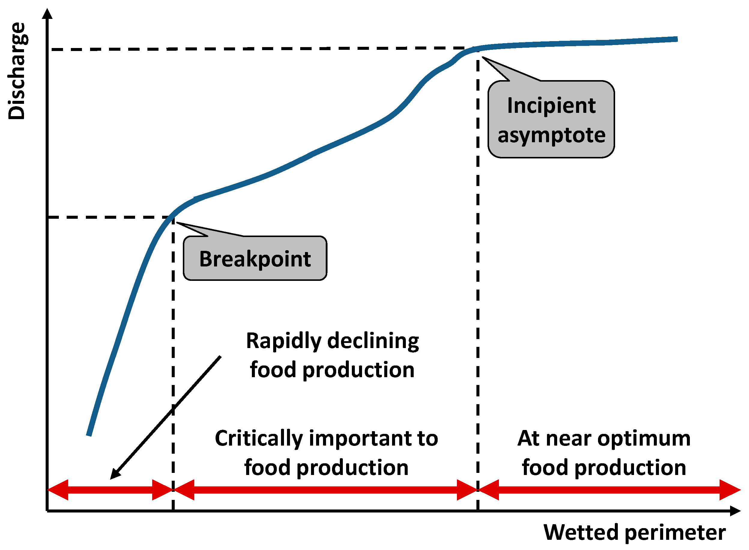
Hydraulic rating methods can be viewed as preliminary appearances of habitat simulation or even holistic approaches [1]. Since the available aquatic habitat, for given flow conditions, is mainly determined by the wetted perimeter of the channel, several methods have been proposed aimed at using the above geometrical characteristic as a basic tool for ecological evaluation. The key idea is that the wetted perimeter of shallow and wide rivers is more sensitive to flow changes, than narrow and deep ones [3]. In this context, the wetted perimeter–discharge breakpoint has been extensively used to define optimum or minimum flows for fish rearing in the USA, from the mid-1970s. The breakpoint (also referred to as the inflection point) is the point where the slope of the stage–discharge curve changes (decreases), so that a large increase in flow results in a small increase in perimeter. The lowest breakpoint in the curve is taken to represent a critical discharge below which habitat conditions for aquatic organisms rapidly become unfavorable [20,21].
Nowadays, the use of hydrological indices or the wetted perimeter as unique indicators of the river health, and the means for determining ecological flows, is limited. In this respect, hydrological and hydraulic approaches are usually employed only in conjunction with process-based techniques that also account for water quality and biological criteria. For instance, habitat simulation methods assess the environmental flow requirements on the basis of detailed analyses of the quantity and suitability of instream physical habitat, particularly target species or assemblages (mainly fish), that are observed under different flow regimes. These use hydrological, hydraulic and biological data, at representative sites along the rivers, to represent the habitat conditions within hydraulic simulation tools, thus allowing for the establishment of a direct link between habitat and discharge. A well-known approach in this category is the instream flow incremental methodology (IFIM) [22], which has been considered by some practitioners as the most scientifically and legally defensible methodology for assessing environmental flows [1]. IFIM was designed to address a number of ecological components (including flow regime, physical habitat structure, water quality, and energy fluxes) in the context of management decisions; for this reason, it also comprises mechanisms for analyzing the institutional aspects of water resource issues. Typically, the minimum acceptable flow is established according to predictions of instream habitat availability that are matched against preferences of one or a few species of fish, using hydraulic and habitat rating methods, such as in-stream transect analysis and the Physical Habitat Simulation (PHABSIM) software, developed by the USGS [23] (which is major component of IFIM).
Finally, the so-called holistic methods—a term introduced by Arthington et al. [24]—are essentially decision-making processes that allow scientists and stakeholders from multiple disciplines to share data and knowledge [25], thus indicating a shift from prescriptive to interactive approaches [1]. Their rationale is based on the same philosophy, imposing that all major abiotic and biotic components constitute the river ecosystem to be managed and the full spectrum of flows, in terms of their temporal and spatial variability, constitute the flows to be managed. Obviously, these approaches are much more demanding in terms of data requirements as well as human and time resources, since their objective is to address the requirements of the entire riverine ecosystem, comprising instream and groundwater systems, floodplains and downstream receiving waters [25]. In fact, they do not provide explicit ecological targets but rather focus on determining the effects of water resources management scenarios, thus being suitable for related studies and master plans. In the last two decades, a wide range of such methodologies has been developed and applied, initially in Australia and South Africa, and more recently in the UK. The most recognized ones are the building block method [26,27], the Downstream Response to Imposed Flow Transformations (DRIFT) framework [24], and the benchmarking method [2,28].
DRIFT is an interactive EFA approach, developed and applied within several water resources development projects in Africa. Based on a comprehensive data-management process, it provides flow scenarios and descriptive summaries of their consequences, in terms of the condition of river ecosystems, for examination and comparison by decision makers. These are then used to determine desired future conditions and the relevant instream flow requirements. DRIFT is made up of four modules, i.e., biophysical, sociological, scenario development and economic. The first evaluates the present nature and functioning of the ecosystem, and provides predictions of how these will change under a range of different flow manipulations. The second module identifies subsistence users at risk from flow manipulations and quantifies their links with the river. In the third module, the outputs from the first two are brought together to produce the biophysical and subsistence scenarios, while the fourth module addresses the costs of mitigation and compensation.
As mentioned in the Introduction, the proposed approach is actually a simplification of the DRIFT framework, aimed at balancing the holistic but data (and time) demanding approach of the original method with the severe data limitations across the study area (i.e., Lesotho).
3. Study Area
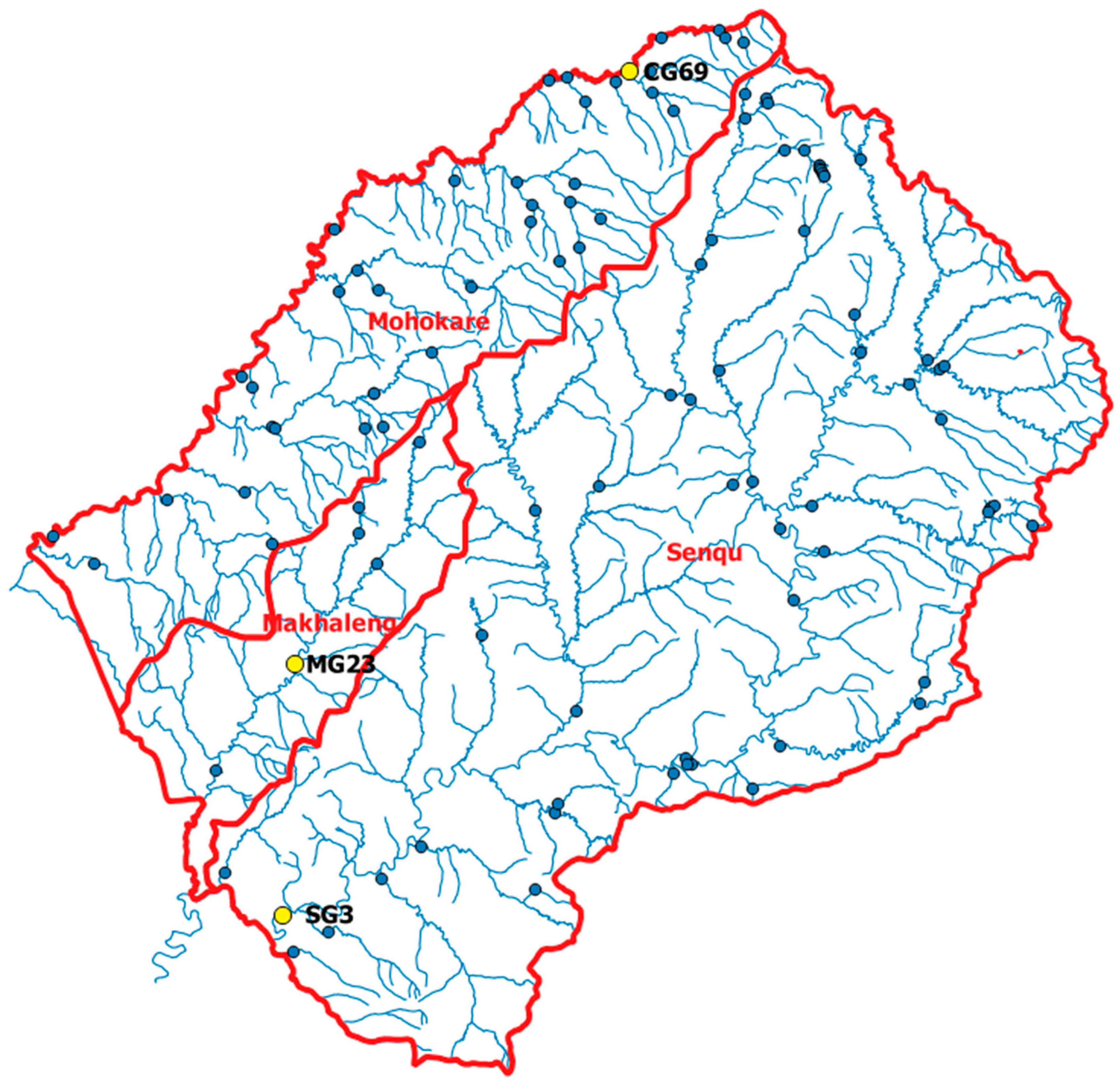
The surface water resources of Lesotho originate from three major rivers and associated catchments, i.e., Mohokare in the west (shared with Republic of South Africa), Makhaleng in the central area, and Senqu in the east. These rivers converge downstream to form the Orange-Senqu River in South Africa, which runs eastwards to the Atlantic Ocean (Figure 1). At present, 69 operational river flow monitoring stations exist across the three rivers.
This study investigated the flow regime at three pilot hydrometric stations, located at strategic sites across each of the three major rivers of Lesotho:
- Station SG3, Senqu River at Seaka Bridge (data period: 1972–2011)
- Station CG69, Mohokare River at Ha Mabine (data period: 1988–2011)
- Station MG23, Makhaleng River at Ha Qaba (data period: 1981–2011)
As shown in Figure 1, the three stations monitor the runoff generated from drainage areas of substantially different extent. In particular, station SG3 (Seaka Bridge) is located close to the outlet of the Senqu River, station MG23 (Ha Qaba) is located in the middle of Mahkaleng River, while station CG69 (Ha Mabine) is located in the upper course of Mohokare River. Table 1 contains summary information for the three sites of interest. At each site, we collected daily flow time series and cross-section geometry data, which are used within the hydrological and hydraulic analyses, respectively.
4. Materials and Methods
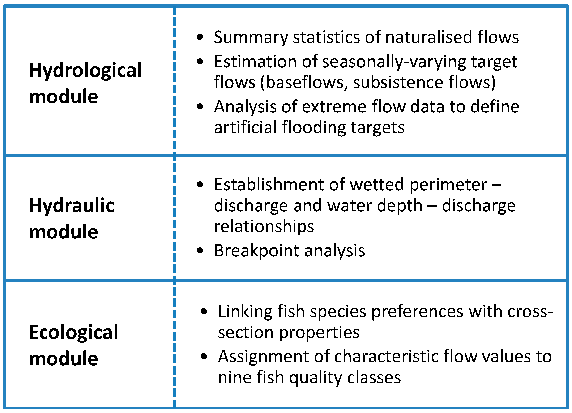
A holistic, data-driven, EFA framework is proposed, taking advantage of the available data and survey information. Following the rationale of the DRIFT approach, this framework comprises three modeling steps, hereafter referred to as “modules”, accounting for hydrological, hydraulic and ecological (fish habitat) issues, respectively, as schematically represented in Figure 2. The three modules are further explained in the following sections.
4.1. Hydrological Module
This module consists of two levels of analysis, based on monthly average and daily average data, respectively. At the first level, we define a range of desirable flow fluctuation between the minimum and the mean monthly flow. At the second level, we define critical flow values per month, identified following the general concepts proposed by the Texas National Research Council [29]. The latter separates long-term hydrographs into flow components, called subsistence, base, high-flow pulse and overbank [30]. “Analogs” of the first two components were identified by constructing the flow duration curves for each month and estimating critical flow quantiles, while for the last two components, we used outcomes of the extreme analysis. More specifically:
Subsistence flows: Subsistence flows are associated with low flow dynamics and they can also be regarded as the lower threshold for water quality protection. Usually, these are estimated by calculating seasonal Q95 values (i.e., flows that are exceeded 95% of the time in each season based on the full data set). In this study, for all pilot sites, we selected the daily Q97, i.e., the value that is exceeded 97% of time (approximately, all except one day per month).
Baseflows: The typical suite includes the selection of characteristic percentiles, corresponding to low, medium and high (or dry, average and wet) baseflow levels. In this study, we employed the flow quantiles Q60, Q75, and Q90.
High-flow pulses and overbank events: According to Opdyke et al. [30], high-flow pulses and floods (collectively termed “episodic events”) are distinguished by whether or not the event’s peak flow exceeds the estimate of bankfull discharge. In this study, we defined, as analogs of high-flow pulses and floods, the corresponding maximum daily flows, with return periods of two and five years. The above values are estimated through statistical analysis of annual daily maxima at the three stations, using statistical predictions through the Gumbel distribution function. We remark that an artificial flooding schedule should be carefully designed to favor key components of the river’s ecosystem, such as floodplain vegetation, sediment transport, etc.
4.2. Hydraulic Module
The breakpoint of the wetted perimeter versus discharge relationship, also known as the point of inflection (Figure 3), defines a generally accepted flow value, which is crucial for environmental restoration and fish food production. This method is the most parsimonious in terms of data requirements, since it only requires elementary information about the river geometry, thus also being suitable for ungauged rivers. In preliminary EFA studies, the breakpoint approach has been successfully employed in heavily modified rivers, providing very reliable results [7]. In this study, using the Manning’s equation, we employed the maximum curvature procedure, by Gippel and Stewardson [20], to define the lower breakpoint of all examined rating curves.
4.3. Ecological Module
Within an earlier implementation of DRIFT across Lesotho Highlands rivers, Arthington et al. [2] employed seasonal field surveys to provide a detailed set of flow-related ecological requirements for representative fish species and development stages, known or expected to occur at several study sites. The key species included Maloti minnow, Rock catfish, Smallmouth yellowfish, Largemouth yellowfish, Orange River mudfish, Trout, Moggel, and Chubhead, which were further classified into sub-categories, i.e., adults, juvenile and habitat. This dataset provided the bulk of the biological information used to assess the consequences of modified flow regimes for all expected fish species across Lesotho rivers. The preferences of fish species and sub-species were quantified by means of stream habitat characteristics (width, depth, velocity, substrate characteristics, instream cover, and bank cover) and water quality parameters (temperature, conductivity, dissolved oxygen, and pH). A summary of this information, in terms of desirable ranges of water depth, is shown in Table 2.
For a given river section, the three characteristic water depth values (min, max, medium) per species can be easily expressed in terms of desirable flow rates, using a common hydraulic approach, e.g., a rating curve. Hence, the ecological requirements of different fish species and development stages, expressed in terms of the generally-recommended water depth ranges across Lesotho, are “translated” as three characteristic flow values (min, max, medium) that are site-specific.
As shown in Table 2, the recommended water depth ranges fluctuate significantly across the different fish species and their developmental stage. For instance, the upper desirable water depth for the adult Trout is 2.5 m, while for the adult Maloti minnow, it is only 0.3 m. Apparently, these large differences would also result in substantially different flow requirements, which directed us to employing a statistical approach to link fish preferences with flows.
In this respect, also following the rationale of DRIFT, we propose a classification, by means of a conceptual statistical fish quality index ranging from 1 to 9, which represents an overall score of the river section conditions against critical discharge values (Table 3). The computational procedure is relatively straightforward, since it only employs elementary statistical operations over the three flow data sets, i.e., the 13 values of min, max, and medium flows, for the corresponding species of Table 2.
The statistical operations for estimating the critical flow values corresponding to each of the nine fish quality indices, are defined in Table 3. For instance, the lowest class, for which we assign a fish index value equal to one, refers to the global minimum flow (and associated depth) of the full sample of fish species, while the second class refers to the minimum over all medium flows. In our approach, we consider that the first two classes refer to moderate fish habitat quality conditions, thus the associated critical flow values are marginally acceptable. Classes 3–6 refer to good fish conditions, while the upper three classes correspond to excellent quality.
5. Results
5.1. Hydrological Analysis
At each of the three pilot stations, we employed extended analyses of raw daily flow data:
- Estimation of key statistical characteristics at daily, monthly and annual time scales;
- Plotting of daily flow – duration curves and estimation of characteristic quantiles; and
- Statistical analysis of annual extremes (minima, maxima).
Since the hydroclimate regime of Lesotho exhibits significant variability across seasons, within the preliminary context of hydrological investigations, we considered different environmental policies for wet and dry months. In this respect, we have proposed desirable flow ranges that follow the variability of the corresponding naturalized flows, by means of monthly target flow values per station, the calculations of which are explained in Section 4.1.
Furthermore, in accordance with modern concepts of EFA, highlighting the major advantages of occasional artificial flooding, we imposed periodical flow releases to be implemented once per year and once per five years. As explained in Section 4.1, these are referred to as high flow pulses and overbank floods, respectively, and they were derived through statistical analysis of maximum daily flows. The proposed releases should be employed during wet periods, in order to be in line with important ecological processes (fish migration, spawning, etc.) and thus avoid detrimental impacts. Considering the natural flow regime at the three sites, artificial floods should be preferably released between December and February.
5.2. Hydraulic Analysis
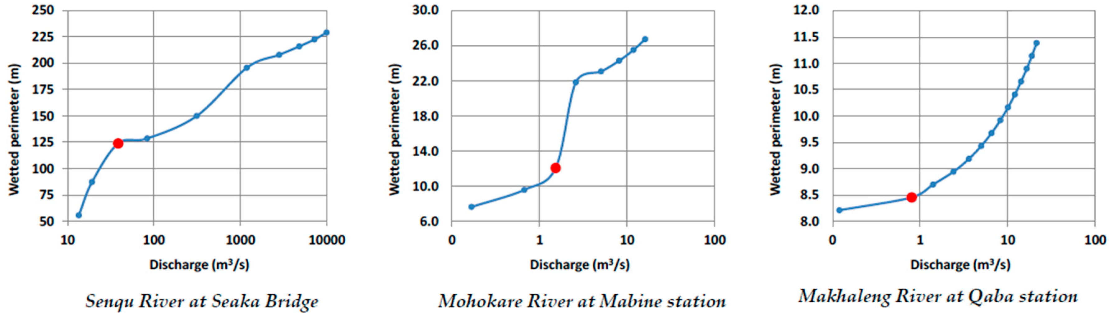
This modeling step was initially aimed at quantifying the hydraulic characteristics at the three pilot cross-sections, by establishing analytical relationships of the wetted perimeter vs. discharge and water depth vs. discharge (the latter was used in ecological analysis, as explained in next section). The calculations were based on the Manning’s formula. Next, following the methodology of Section 4.2, we recognized the lowest breakpoint of the discharge–wetted perimeter curve (i.e., first point where the curve slope changes) at the three cross-sections of interest (Figure 4). The resulting target flows are 38.7 m3/s for Senqu River, 1.5 m3/s for Mohokare River, and 0.8 m3/s for Makhaleng River.
5.3. Ecological Analysis
In general, this task involved the analysis of several hydro-ecosystem components, including fish, macro-invertebrates, geomorphology, instream and floodplain vegetation etc., as well as their influence against alterations of the naturalized discharge. For this purpose, we investigated the fish health dynamics via in situ surveys. A key outcome of this analysis was a direct linking of fish needs against discharge and water depths at each river cross section, by means of fish quality indices.
Following the methodology in Section 4.3, at each study station, for all fish species of interest, through the site-specific stage–discharge relationship, we estimated the flows required to ensure the lower, upper and median depth values of Table 2. Next, we employed the proposed classification, by assigning fish quality indices that correspond to nine critical flow values, as given in Table 4.
An interesting remark for all cases is that, by moving from Class 4 to Class 5, which represents good conditions, the critical flow increases almost one order of magnitude. In contrast, only a slight increase of flow is required to move from Class 3 to Class 4. In this respect, we consider as the benchmark baseflow, the so-called Average_Min, i.e., the average over all flow minima (i.e., flow values corresponding to the lower desirable depths), which represents the critical flow associated with Class 4 (see definition of Table 3). On the other hand, as the marginally acceptable threshold, we consider the so-called Min_Median that corresponds to Class 2. As shown herein, this value was used as a constraint within the proposed environmental flow policy.
5.4. Proposed Environmental Flow Policy
Based on the outcomes of the three aforementioned modules, we proposed a comprehensive flow policy comprising: (a) two artificial flooding targets, referred to as high flow pulse and overbank flood, to be implemented one per year and once per five years, respectively; (b) ranges of monthly baseflows, in terms of desirable minimum, medium and maximum flow values; and (c) monthly subsistence flows, representing an absolutely essential flow to be maintained per month.
In particular, the monthly baseflows were derived as follows:
- the max monthly baseflow as the daily flow quantile Q60 of the corresponding month;
- the median monthly baseflow as the daily flow quantile Q75 of the corresponding month; and
- the min monthly baseflow as the larger value among the daily flow quantile Q90 of the corresponding month and the Min_Medium critical flow, corresponding to Fish Quality Class = 2.
6. Evaluation of Proposed Environmental Flow Policy
6.1. Comparison against Historical Flow Data of Senqu River at Seaka Bridge
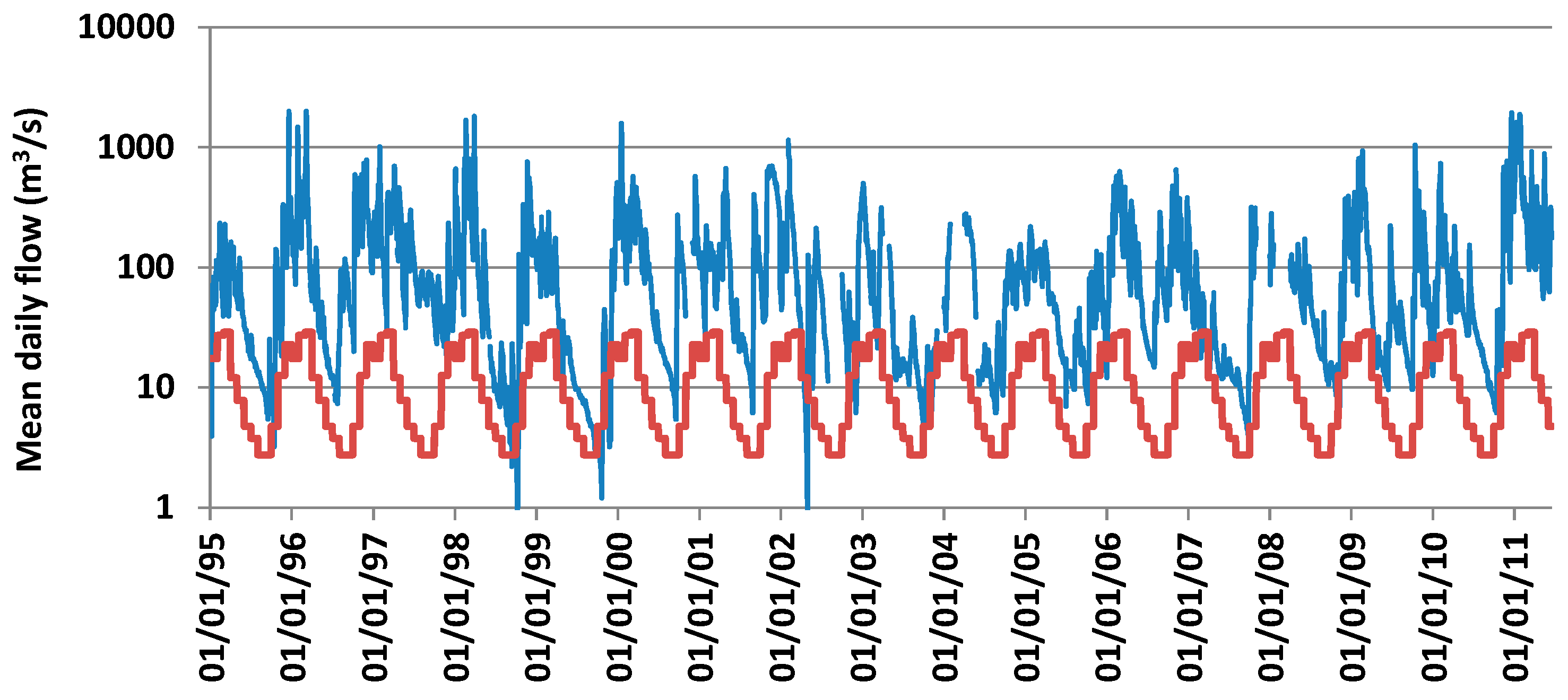
For the evaluation of the proposed environmental policy, we took advantage of available flow data for the Senqu River at Seaka Bridge during 1995–2011, when the flows were partially regulated due to the operation of the upstream Katse dam. In this respect, we compared the actual flows with the desirable, seasonally-varying, minimum EF baseflow thresholds of Table 4. As shown in Figure 5, these values are generally satisfied, with few exceptions, mainly occurring during the wet period.
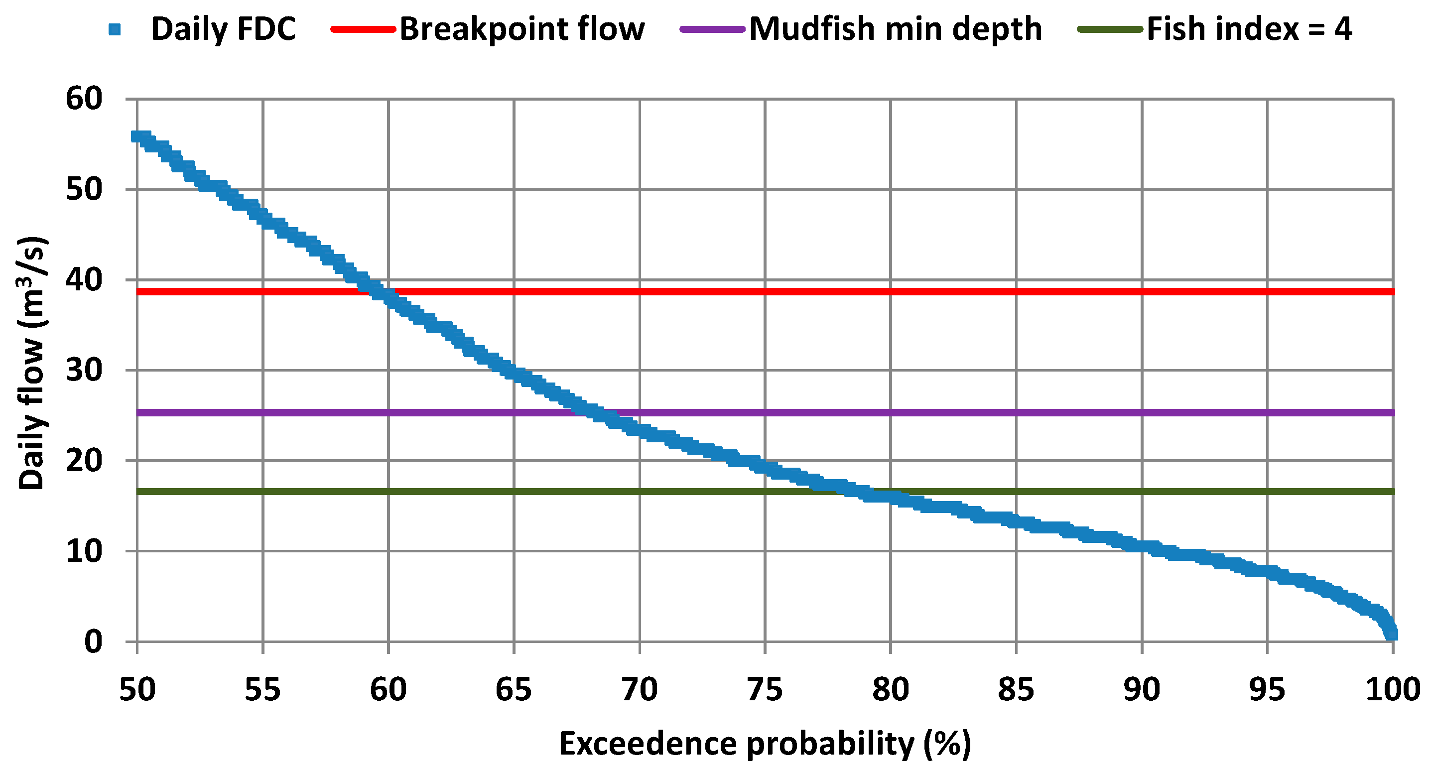
For convenience, we also accounted for three characteristic constant flow thresholds, namely:
- the value of 38.7 m3/s, defined through the hydraulic analysis as corresponding to the breakpoint of the wetted perimeter–discharge curve;
- the value of 25.3 m3/s, which corresponds to the minimum desirable depth for the adult Orange River Mudfish, i.e., 30 cm; and
- the value of 16.6 m3/s, defined through the conceptual statistical fish index approach as corresponding to an index value of 4.
In Figure 6, we contrast the above three values against the daily flow duration curve, which also allows estimation of the non-exceedance probability of the above thresholds. Specifically, 40% of the time, the daily flow is lower than the largest value, estimated through the breakpoint analysis. Thirty-two percent of the time, it is lower than the desirable threshold for the adult Orange River Mudfish, while 21% of the time, it is lower than the critical flow corresponding to a fish index value of 4.
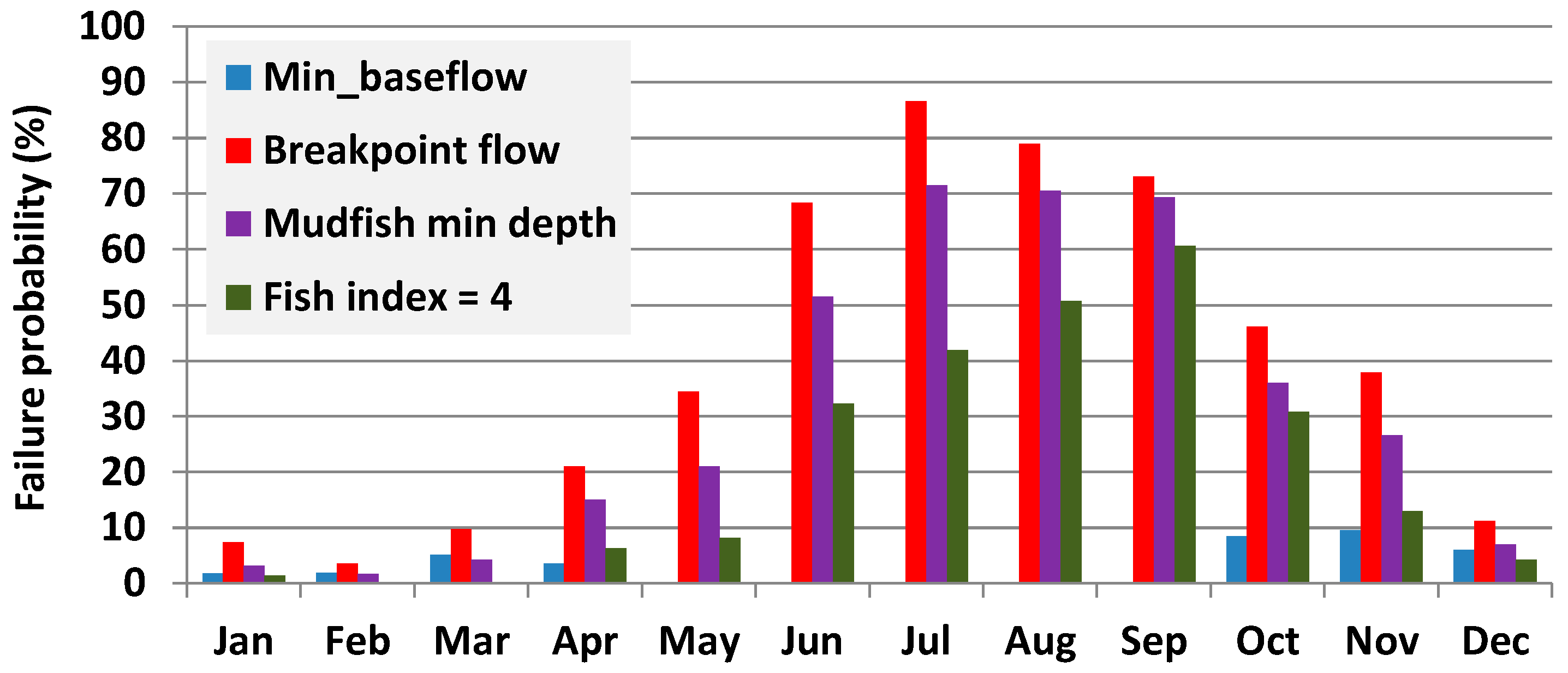
In Figure 7, we also plot the monthly failure probabilities with respect to the aforementioned thresholds, both constant and seasonally-varying. As shown, the minimum baseflow target is fully satisfied during the dry period (from May to September) while during the wet period, the river flow is lower than the desirable value for a relatively small percentage of the time. The larger deviations appear during October and November, when the failure probability reaches 10%, which is envisaged to be due to flow regulations across the upstream hydrosystem. The corresponding failure probabilities would be much larger if a constant flow threshold was used, represented as breakpoint flow in Figure 7. As it would result in a lower failure rate, a more reasonable limit would be the application of the benchmark flow corresponding to Fish Quality Index 4. On the other hand, the Mudfish min depth would provide a more stringent flow requirement and therefore results in a higher failure rate.
6.2. Impacts on Sediment Rate Regime at Mabine Station
The maintenance of the sediment regime is critical for the riverine/riparian environment and any changes to flow/sediment can affect habitats and organisms [31,32]. To validate the proposed EF release, we also carried out a simplified sediment analysis at Mabine Station, where both sediment and flow data were available at daily intervals. These datasets were used to establish monthly-varying relationships of sediment rates vs. discharge. A key assumption of our analysis is that the parameters of these statistical relationships will not be significantly influenced by future regulations. Under this premise, we initially generated synthetic flow data that preserve the statistical patterns of the proposed environmental policy, as quantified in Table 6, and next applied the aforementioned relationships to estimate the anticipated sediment rates.
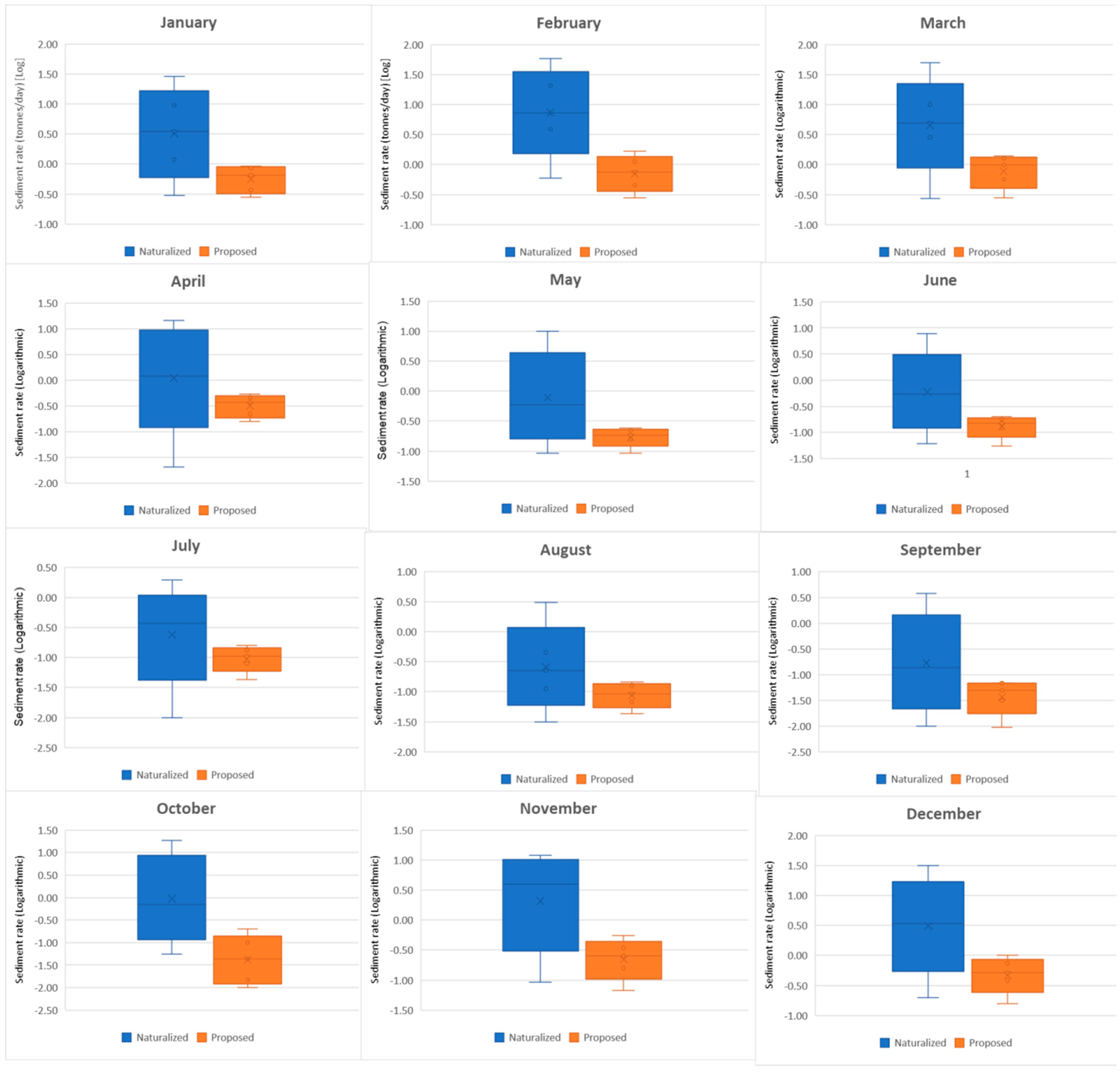
In Figure 8, we represent the historical vs. synthetic sediment rate data by means of box-plots. It can be seen that under the proposed EF, the sediment rates will exhibit much less variability throughout the year, especially during the wet months (May–September). This is due to the overall reduction in discharge, which will be generally maintained within the recommended minimum and maximum values of Table 6. Obviously, this will lead to significant reduction of sediment transport at Mabine station, yet for most months, the synthetically-generated patterns are still within the statistical ranges of the observed data. Moreover, we expect that grace to artificial flooding, to be implemented as one flow release per year (overbank flooding) and one release per five years (high flow pulse). We will occasionally ensure much higher rates of sediment transport, which will be beneficial for the river and riparian environment.
For the two months exhibiting the largest deviation from the observed patterns, i.e., February and October, we revised the proposed environmental policy, on the basis of the statistical outcomes of Figure 8. In this vein, we proposed to increase the recommended minimum EF flows for these months, to better represent the sedimentation regime under natural flow conditions. In particular, for February, we proposed to assign a minimum EF up to 0.60 instead of 0.22 m3/s, while for October we proposed to slightly increase the minimum EF to 0.20 instead of 0.15 m3/s. As shown in Table 6, the latter is the so-called Min_Medium critical flow (i.e., the flow ensuring Fish Quality Class 2) and not the Q90, which is only 0.01 m3/s. We reiterate that, in our methodology, as an estimator of the minimum EF, we use the largest of Q90 and the Min_Medium.
7. Conclusions
The main objective of this study was to provide an environmental flow policy at three pilot sites in Lesotho, located across the main watercourses of the country. Our methodology follows the rationale and concepts of state-of-the-art environmental flow assessment approaches, particularly the well-known DRIFT method, at the same time being more parsimonious and easier to implement. In this respect, it was adapted to local conditions using the available data (hydrological, hydraulic, and ecological) and abstract information of fish habitat preferences based on field surveys.
A new dynamic approach was proposed, linking several components of the riverine environment in conjunction with hydrological, hydraulic and ecological criteria and environmental restrictions, to provide a dynamic environmental flow policy that consists of:
- A monthly-varying range of target flow releases that follows the physical regime, which can be seen as a reconstruction “mimic” of the total river environment restoration.
- An artificial flooding schedule, by means of releasing extreme daily flows corresponding to return periods of two and five years, which are essential for maintaining crucial river elements, such as floodplain vegetation and sediment refreshment.
- A novel conceptual approach for fish quality classification, which links water depths and associated flow thresholds with habitat characteristics, for a wide range of fish species.
The overall approach was employed at three representative river sections across Lesotho, draining catchments of different extent, and was next validated using long-term records of flow and sediment samples at two out of there pilot sites. Since different approaches provide (as expected) a wide range of target flow values, a synthesis of criteria is essential in establishing a proper EF policy. The major contribution of this research is the direct expression of a specific flow value with a fish quality index, which allows easy quantification of the impacts of the selected policy to the aquatic environment. The quite large range of target baseflow values per season, generally expressed in terms of Q90 (minimum) and Q60 (maximum), ensures flexibility for water managers, while occasional deviations are acceptable, through the concept of subsistence flows, estimated as the Q97.
An interesting conclusion of the combined analyses is that in most cases, the target value Q90 exceeds the so-called Min_Medium flow that corresponds to Fish Quality Class 2. Nevertheless, it is strongly recommended that the largest of the two flow values is employed. As shown in the case of Mabine station, the implementation of a stricter EF target, together with a carefully planned artificial flooding schedule, also favors the sedimentation processes, which is a very important component of the overall health of the downstream riverine system.
However, an even more beneficial EF policy is to assign, as a baseflow target, the critical flow that corresponds to Fish Quality Class 4, i.e., the Average_Min. Interestingly, at all examined stations, the latter is comparable with the lowest breakpoint on the wetted perimeter–discharge curve. This conclusion, which should obviously be validated in more studies worldwide, may imply that the two approaches, i.e., hydraulic and ecological, converge to similar outcomes. If this hypothesis is valid, although receiving reasonable criticism [33], the problem of EF assessment, at least in a preliminary context, would be substantially simplified, since the breakpoint analysis is very simple, only requiring the use of easily-retrieved cross-section geometry data and the implementation of trivial hydraulic calculations.
Author Contributions
A.T. was responsible for the data mining, the model development and draft writing; W.S. was responsible for model reviewing and reporting; N.G. was responsible for processing and reporting; Y.K. was responsible for the coordination of the whole project; and A.E. was responsible for model development and overall supervision of the manuscript.
Funding
This paper was part of the project “Classification of Water Courses and Determination of Environmental Flow Requirements Study in Lesotho Bid Reference LWSIP II/Comp III/C/19-2015” funded by the World Bank. The authors are grateful to the Client and the local Authorities for their support during the project implementation.
Acknowledgments
The authors are grateful to “Arup University” for its support on this study and to Ken Leahy, Associate Director at Arup for his valuable comments. We are grateful to the reviewers, editors and Editor in Chief Professor Bordalo, who helped us to improve substantially our work. This work is dedicated to the memory of a great scientist, Don Tennant, who spent his life studying the Environmental Flows under mainly hydrological techniques.
Conflicts of Interest
The authors declare no conflict of interest.
References
- Tharme, R.E. A global perspective on environmental flow assessment: Emerging trends in the development and application of environmental flow methodologies for rivers. River Res. Appl. 2003, 19, 397–441. [Google Scholar] [CrossRef]
- Arthington, A.H.; Rall, J.L.; Kennard, M.J.; Pusey, B.J. Environmental flow requirements of fish in Lesotho rivers using the DRIFT methodology. River Res. Appl. 2003, 19, 641–666. [Google Scholar] [CrossRef]
- Acreman, M.C.; Dunbar, M.J. Defining environmental river flow requirements—A review. Hydrol. Earth Syst. Sci. 2004, 8, 861–876. [Google Scholar] [CrossRef]
- Suen, J.P.; Eheart, J. Reservoir management to balance ecosystem and human needs: Incorporating the paradigm of the ecological flow regime. Water Resour. Res. 2006, 42. [Google Scholar] [CrossRef] [Green Version]
- Tyralis, H.; Tegos, A.; Delichatsiou, A.; Mamassis, N.; Koutsoyiannis, D. A perpetually interrupted interbasin water transfer as a modern Greek drama: Assessing the Acheloos to Pinios interbasin water transfer in the context of integrated water resources management. Open Water J. 2017, 4, 11. [Google Scholar]
- Smakhtin, V.U.; Shilpakar, R.L.; Hughes, D.A. Hydrology-based assessment of environmental flows: An example from Nepal. Hydrol. Sci. J. 2006, 51, 207–222. [Google Scholar] [CrossRef]
- Efstratiadis, A.; Tegos, A.; Varveris, A.; Koutsoyiannis, D. Assessment of environmental flows under limited data availability—Case study of Acheloos River, Greece. Hydrol. Sci. J. 2014, 59, 731–750. [Google Scholar] [CrossRef]
- Tegos, M.; Nalbantis, I.; Tegos, A. Environmental flow assessment through integrated approaches. Eur. Water 2017, 60, 167–173. [Google Scholar]
- Petts, G.E. Instream flow science for sustainable river management. J. Am. Water Resour. Assoc. 2009, 45, 1071–1086. [Google Scholar] [CrossRef]
- Acreman, M.C.; Overton, I.C.; King, J.; Wood, P.; Cowx, I.G.; Dunbar, M.J.; Kendy, E.; Young, W. The changing role of ecohydrological science in guiding environmental flows. Hydrol. Sci. J. 2014, 59, 433–450. [Google Scholar] [CrossRef] [Green Version]
- Zeiger, S.J.; Hubbart, J.A. Assessing environmental flow targets using pre-settlement land cover: A SWAT modeling application. Water 2018, 10, 791. [Google Scholar] [CrossRef]
- Tennant, D.L. Instream flow regimens for fish, wildlife, recreation and related environmental resources. Fisheries 1976, 1, 6–10. [Google Scholar] [CrossRef]
- Acreman, M.C.; Dunbar, M.J.; Hannaford, J.; Mountford, O.; Wood, P.; Holmes, N.; Cowx, I.; Noble, R.; Extence, C.; Aldrick, J.; et al. Developing environmental standards for abstractions from UK rivers to implement the EU water framework directive. Hydrol. Sci. J. 2008, 53, 1105–1120. [Google Scholar] [CrossRef]
- Smakhtin, V.U. Low flow hydrology: A review. J. Hydrol. 2001, 240, 147–186. [Google Scholar] [CrossRef]
- Palau, A.; Alcázar, J. The basic flow: An alternative approach to calculate minimum environmental instream flows. In Proceedings of the 2nd International Symposium on Habitat Hydraulics, Québec City, QC, Canada, 11–14 June 1996; Volume A, pp. 547–558. [Google Scholar]
- Richter, B.D.; Baumgartner, J.V.; Powell, J.; Braun, D.P. A method for assessing hydrologic alteration within ecosystems. Conserv. Biol. 1996, 10, 1163–1174. [Google Scholar] [CrossRef]
- Richter, B.D.; Baumgartner, J.; Wigington, R.; Braun, D. How much water does a river need? Freshwater Biol. 1997, 37, 231–249. [Google Scholar] [CrossRef]
- Ge, J.; Peng, W.; Huang, W.; Qu, X.; Singh, S.K. Quantitative assessment of flow regime alteration using a revised range of variability methods. Water 2018, 10, 597. [Google Scholar] [CrossRef]
- Poff, N.L.; Richter, B.D.; Arthington, A.H.; Bunn, S.E.; Naiman, R.J.; Kendy, E.; Henriksen, J. The ecological limits of hydrologic alteration (ELOHA): A new framework for developing regional environmental flow standards. Freshwater Biol. 2010, 55, 147–170. [Google Scholar] [CrossRef]
- Gippel, C.J.; Stewardson, M.J. Use of wetted perimeter in defining minimum environmental flows. Regul. Rivers Res. Manag. 1998, 14, 53–67. [Google Scholar] [CrossRef]
- Standard Operating Procedure for the Wetted Perimeter Method in California; CDFW Instream Flow Program Standard Operating Procedure DFG-IFP-004; California Department of Fish and Wildlife: Sacramento, CA, USA, 2013; p. 19.
- Stalnaker, C.B.; Lamb, B.L.; Henriksen, J.; Bovee, K.; Bartholow, J. The Instream Flow Incremental Methodology: A Primer for IFIM; Geological Survey Biological Report; National Wildlife Research Center: Fort Collins, CO, USA, 1995; pp. 29–45. [Google Scholar]
- Waddle, T.J. PHABSIM for Windows: User’s Manual and Exercises; U.S. Geological Survey; USGS Publications Warehouse: Fort Collins, CO, USA, 2001; p. 288. [Google Scholar]
- Arthington, A.H.; King, J.M.; O’Keefe, J.H.; Bunn, S.E.; Day, J.A.; Pusey, B.J.; Bluhdorn, D.R.; Tharme, R. Development of a holistic approach for assessing environmental flow requirements of riverine ecosystems. In Proceedings of an International Seminar and Workshop on Water Allocation for the Environment; Pigram, J.J., Hooper, B.P., Eds.; Centre for Water Policy Research, University of New England: Armidale, Australia, 1992; pp. 69–76. [Google Scholar]
- King, J.; Brown, C.; Sabet, H. A scenario-based holistic approach to environmental flow assessments for rivers. River Res. Appl. 2003, 19, 619–639. [Google Scholar] [CrossRef]
- King, J.M.; Tharme, R.E. Assessment of the Instream Flow Incremental Methodology and Initial Development of Alternative Instream Flow Methodologies for South Africa; Water Research Commission Report No. 295/1/94; Water Research Commission: Pretoria, South Africa, 1994. [Google Scholar]
- King, J.; Louw, D. Instream flow assessments for regulated rivers in South Africa using the building block methodology. Aquat. Ecosyst. Health Manag. 1998, 1, 109–124. [Google Scholar] [CrossRef]
- Arthington, A.H.; Zalucki, J.M. Comparative Evaluation of Environmental Flow Assessment Techniques: Review of Methods; LWRRDC Occasional Paper Series 27/98; Land and Water Resources Research and Development Corporation: Canberra, Australia, 1998; p. 141. [Google Scholar]
- National Research Council. The Science of Instream Flows: A Review of the Texas Instream Flow Program; The National Academies Press: Washington, DC, USA, 2005. [Google Scholar]
- Opdyke, D.R.; Oborny, E.L.; Vaugh, S.K.; Mayes, K.B. Texas environmental flow standards and the hydrology-based environmental flow regime methodology. Hydrol. Sci. J. 2014, 59, 820–830. [Google Scholar] [CrossRef] [Green Version]
- Norris, R.H.; Thoms, M.C. What is river health? Freshwater Biol. 1999, 41, 197–209. [Google Scholar] [CrossRef]
- Zingraff-Hamed, A.; Noack, M.; Greulich, S.; Schwarzwälder, K.; Pauleit, S.; Wantzen, K.M. Model-based evaluation of the effects of river discharge modulations on physical fish habitat quality. Water 2018, 10, 374. [Google Scholar] [CrossRef]
- Theodoropoulos, C.; Georgalas, S.; Mamassis, N.; Stamou, A.; Rutschmann, P.; Skoulikidis, N. Comparing environmental flow scenarios from hydrological methods, legislation guidelines and hydrodynamic habitat models downstream of the Marathon Dam (Attica, Greece). Ecohydrology 2018. [Google Scholar] [CrossRef]
Figure 1.
Catchment boundaries (red lines), hydrographic network and flow monitoring stations (blue points) across Lesotho (the three pilot stations are highlighted in yellow).
Figure 1.
Catchment boundaries (red lines), hydrographic network and flow monitoring stations (blue points) across Lesotho (the three pilot stations are highlighted in yellow).

Figure 2.
Flowchart of the proposed EFA framework.

Figure 3.
Example of wetted perimeter–discharge curve showing relationship between breakpoints and fish food production (adapted by CDFW [21]).
Figure 3.
Example of wetted perimeter–discharge curve showing relationship between breakpoints and fish food production (adapted by CDFW [21]).

Figure 4.
Semi-logarithmic plots of wetted perimeter vs. discharge at the three pilot sites of interest, highlighting the lowest breakpoint (change of slope).
Figure 4.
Semi-logarithmic plots of wetted perimeter vs. discharge at the three pilot sites of interest, highlighting the lowest breakpoint (change of slope).

Figure 5.
Daily flow time series of Senqu River at Seaka Bridge during 1995–2011 (semi-logarithmic plot) against monthly minimum baseflow values defined in the context of EFA.
Figure 5.
Daily flow time series of Senqu River at Seaka Bridge during 1995–2011 (semi-logarithmic plot) against monthly minimum baseflow values defined in the context of EFA.

Figure 6.
Comparison of flow-duration curve (blue line) of Senqu River at Seaka Bridge for 1995–2011 against critical flow thresholds defined in the context of EFA (the lower part of the curve is shown, corresponding to flows lower than the median, thus exhibiting exceedance probability >50%).
Figure 6.
Comparison of flow-duration curve (blue line) of Senqu River at Seaka Bridge for 1995–2011 against critical flow thresholds defined in the context of EFA (the lower part of the curve is shown, corresponding to flows lower than the median, thus exhibiting exceedance probability >50%).

Figure 7.
Monthly failure probabilities (%) using four flow categories defined in the context of EFA.
Figure 7.
Monthly failure probabilities (%) using four flow categories defined in the context of EFA.

Figure 8.
Monthly box plots for sediment rates at Mabine Station for natural conditions (observed data) and considering simulated data under the proposed EF policy (t/day, in logarithmic scale).
Figure 8.
Monthly box plots for sediment rates at Mabine Station for natural conditions (observed data) and considering simulated data under the proposed EF policy (t/day, in logarithmic scale).


Table 1.
Summary data of pilot monitoring stations.
| Station Name/Code | Seaka Bridge (SG3) | Ha Mabine (CG69) | Ha Qaba (MG23) |
|---|---|---|---|
| River | Senqu | Mohokare | Makhaleng |
| Elevation (m) | 1400 | 1600 | 1525 |
| Drainage area (km2) | 19875 | 304 | 1554 |
| Flow data record | 25 August 1972–16 June 2011 | 1 June 1988–31 August 2011 | 11 October 1981–31 March 2011 |
| Daily data values | 12753 | 8241 | 9507 |
| Missing values | 1422 | 251 | 1257 |
| Mean daily flow (m3/s) | 117.9 | 1.82 | 13.1 |
Table 2.
Summary of flow-related ecological requirements of fish species, in terms of ranges of desirable water depths, across Lesotho Highlands rivers, (adapted from [2]).
Table 2.
Summary of flow-related ecological requirements of fish species, in terms of ranges of desirable water depths, across Lesotho Highlands rivers, (adapted from [2]).
| Fish Species | Desirable Water Depth (m) | Medium Value (m) |
|---|---|---|
| Maloti minnow, adult | 0.21–0.30 | 0.26 |
| Maloti minnow, juvenile | 0.05–0.70 | 0.38 |
| Maloti minnow, habitat | 0.20–0.40 | 0.30 |
| Rock catfish, adult | 0.15–0.30 | 0.23 |
| Rock catfish, juvenile | 0.10–0.60 | 0.35 |
| Smallmouth yellowfish, adult | 0.60–2.70 | 1.65 |
| Smallmouth yellowfish, juvenile | 0.10–0.60 | 0.35 |
| Orange River mudfish, adult | 0.30–1.71 | 1.01 |
| Orange River mudfish, juvenile | 0.15–0.60 | 0.38 |
| Orange River mudfish, habitat | 0.10–0.20 | 0.15 |
| Trout, adult | 0.40–2.50 | 1.45 |
| Trout, juvenile | 0.11–0.30 | 0.21 |
| Largemouth yellowfish, adult | 0.20–0.70 | 0.45 |
Table 3.
Definition of fish quality classes.
| Class | Critical Flow | Definition |
|---|---|---|
| 1 | Min_Min | Minimum over all minimum flows |
| 2 | Min_Medium | Minimum over all medium flows |
| 3 | Min_Max | Minimum over all maximum flows |
| 4 | Average_Min | Average over all minimum flows |
| 5 | Max_Min | Maximum over all minimum flows |
| 6 | Average_Medium | Average over all medium flows |
| 7 | Average_Max | Average over all maximum flows |
| 8 | Max_Medium | Maximum over all medium flows |
| 9 | Max_Max | Maximum over all maximum flows |
Table 4.
Critical flow values (m3/s) and associated fish quality classes at the three stations of interest.
Table 4.
Critical flow values (m3/s) and associated fish quality classes at the three stations of interest.
| Fish Quality Class | Seaka Bridge | Mabine | Qaba |
|---|---|---|---|
| 1 | 0.68 | 0.03 | 0.05 |
| 2 | 2.75 | 0.15 | 0.17 |
| 3 | 11.17 | 0.68 | 0.61 |
| 4 | 16.63 | 1.15 | 0.83 |
| 5 | 102.75 | 7.74 | 4.75 |
| 6 | 152.07 | 13.09 | 6.38 |
| 7 | 427.19 | 40.68 | 16.57 |
| 8 | 792.96 | 72.43 | 31.55 |
| 9 | 2144.32 | 215.08 | 79.33 |
Table 5.
Environmental flow values at Seaka Bridge station (m3/s) (1972–2011).
| January | February | March | April | May | June | July | August | September | October | November | December | |
|---|---|---|---|---|---|---|---|---|---|---|---|---|
| High flow pulse | 1132.8 (annual flood) | |||||||||||
| Overbank flood | 1620.8 (5-year maximum flood event) | |||||||||||
| Max baseflow | 47.2 | 121.4 | 85.2 | 45.2 | 21.3 | 14.3 | 9.1 | 6.9 | 12.6 | 28.8 | 62.7 | 70.0 |
| Median baseflow | 27.2 | 72.6 | 51.4 | 28.8 | 13.1 | 8.2 | 5.4 | 3.8 | 7.7 | 15.6 | 32.2 | 44.2 |
| Min baseflow | 17.3 | 27.2 | 28.8 | 12.1 | 7.8 | 4.7 | 3.8 | 2.8 | 2.8 | 4.7 | 12.6 | 22.7 |
| Subsistence flow | 4.0 | 15.4 | 16.0 | 9.1 | 5.4 | 3.5 | 2.9 | 1.8 | 0.9 | 2.9 | 3.5 | 5.3 |
Table 6.
Environmental flow values at Mabine station (m3/s) (1988–2011).
| January | February | March | April | May | June | July | August | September | October | November | December | |
|---|---|---|---|---|---|---|---|---|---|---|---|---|
| High flow pulse | 51.3 (annual flood) | |||||||||||
| Overbank flood | 96.9 (5-year maximum flood event) | |||||||||||
| Max baseflow | 0.68 | 1.19 | 0.95 | 0.40 | 0.19 | 0.16 | 0.13 | 0.12 | 0.06 | 0.16 | 0.47 | 0.78 |
| Median baseflow | 0.44 | 0.58 | 0.56 | 0.27 | 0.15 | 0.13 | 0.11 | 0.08 | 0.04 | 0.05 | 0.22 | 0.33 |
| Min baseflow | 0.21 | 0.22 | 0.22 | 0.15 * | 0.15 * | 0.15 * | 0.15 * | 0.15 * | 0.15 * | 0.15 * | 0.15 * | 0.15 * |
| Subsistence flow | 0.07 | 0.03 | 0.05 | 0.02 | 0.00 | 0.00 | 0.00 | 0.01 | 0.00 | 0.00 | 0.01 | 0.05 |
(*) The Min_Medium flow value is used, since it exceeds the daily Q90 of the corresponding month.
Table 7.
Environmental flow values at Qaba station (m3/s) (1981–2011).
| January | February | March | April | May | June | July | August | September | October | November | December | |
|---|---|---|---|---|---|---|---|---|---|---|---|---|
| High flow pulse | 167.8 (annual flood) | |||||||||||
| Overbank flood | 309.3 (5-year maximum flood event) | |||||||||||
| Max baseflow | 4.6 | 4.8 | 3.9 | 2.1 | 1.7 | 1.5 | 1.3 | 1.1 | 1.5 | 3.7 | 4.7 | 3.7 |
| Median baseflow | 3.0 | 3.2 | 2.4 | 1.6 | 1.2 | 1.1 | 0.9 | 0.9 | 0.9 | 1.8 | 2.8 | 2.3 |
| Min baseflow | 1.4 | 1.3 | 1.5 | 1.1 | 0.8 | 0.6 | 0.3 | 0.6 | 0.6 | 0.9 | 0.9 | 1.1 |
| Subsistence flow | 0.6 | 0.8 | 0.7 | 0.7 | 0.5 | 0.4 | 0.2 | 0.2 | 0.2 | 0.4 | 0.5 | 0.3 |
© 2018 by the authors. Licensee MDPI, Basel, Switzerland. This article is an open access article distributed under the terms and conditions of the Creative Commons Attribution (CC BY) license (http://creativecommons.org/licenses/by/4.0/).
Share and Cite
MDPI and ACS Style
Tegos, A.; Schlüter, W.; Gibbons, N.; Katselis, Y.; Efstratiadis, A. Assessment of Environmental Flows from Complexity to Parsimony—Lessons from Lesotho. Water 2018, 10, 1293. https://doi.org/10.3390/w10101293
AMA Style
Tegos A, Schlüter W, Gibbons N, Katselis Y, Efstratiadis A. Assessment of Environmental Flows from Complexity to Parsimony—Lessons from Lesotho. Water. 2018; 10(10):1293. https://doi.org/10.3390/w10101293
Chicago/Turabian StyleTegos, Aristoteles, Wolfram Schlüter, Niall Gibbons, Yanis Katselis, and Andreas Efstratiadis. 2018. "Assessment of Environmental Flows from Complexity to Parsimony—Lessons from Lesotho" Water 10, no. 10: 1293. https://doi.org/10.3390/w10101293
Note that from the first issue of 2016, this journal uses article numbers instead of page numbers. See further details here.