State of the Art and Recent Advancements in the Modelling of Land Subsidence Induced by Groundwater Withdrawal

Abstract

Land subsidence is probably one of the most evident environmental effects of groundwater pumping. Globally, freshwater demand is the leading cause of this phenomenon. Land subsidence induced by aquifer system drainage can reach total values of up to 14.5 m. The spatial extension of this phenomenon is usually extensive and is often difficult to define clearly. Aquifer compaction contributes to many socio-economic effects and high infrastructure-related damage costs. Currently, many methods are used to analyze aquifer compaction. These include the fundamental relationship between groundwater head and groundwater flow direction, water pressure and aquifer matrix compressibility. Such solutions enable satisfactory modelling results. However, further research is needed to allow more efficient modelling of aquifer compaction. Recently, satellite radar interferometry (InSAR) has contributed to significant progress in monitoring and determining the spatio-temporal land subsidence distributions worldwide. Therefore, implementation of this approach can pave the way to the development of more efficient aquifer compaction models. This paper presents (1) a comprehensive review of models used to predict land surface displacements caused by aquifer drainage, as well as (2) recent advances, and (3) a summary of InSAR implementation in recent years to support the aquifer compaction modelling process.

1. Introduction

Land subsidence is one of the most important environmental effects of groundwater pumping [1,2,3,4,5,6,7]. The proper assessment of the origin, mechanism and impact of this process is a common problem. Globally, the growing demand for fresh water is one of the leading causes of this phenomenon [8]. This is the result of the rapid population growth observed since the 1950s [8,9]. Fresh water for industrial purposes is usually supplied by direct pumping of water from aquifer systems, which have not been contaminated by external factors. This results in the compaction of compressible aquifers [10,11]. Drainage-induced land subsidence values may reach up to 14.5 m [11]. Compacting aquifers contribute to many social and economic disadvantages [12]. The most severe of these include damage to the surface and underground infrastructure and increased risk of flooding in coastal cities [13,14,15].

One of the first documented land subsidence certificates linked to “unspecified geomechanical underground processes” dates back to 1926. It is attributed to W.E. Pratt and D.W. Johnson [16], U.S. geologists conducting ground surface transformation studies induced by oil production in the Goose Creek field in Baytown, Texas. Since then, significant progress has been made in the recognition of the physics of the phenomenon under investigation [11]. Basic hydrogeological and geomechanical concepts have been developed for the aquifer compaction process. In addition, the measurement capacity of land surface displacement has been improved. It is, therefore, possible to determine aquifer compaction more precisely. These activities were crucial in defining models for exploring past and predicting future land surface drainage-induced displacements. Finally, based on the findings of models implemented in this way, initiatives have also been applied to reduce and reverse the environmental and anthropogenic impacts of groundwater pumping [11,17].

Many approaches have been used for the analysis and simulation of aquifer compaction. These include the fundamental relationship between the groundwater head and groundwater flow direction and water pressure and aquifer compaction. Progress in compaction modelling has mainly been related to the development of computer technologies and intensive work on numerical algorithms. These have been carried out since the 1970s. The results of these works have made it possible to solve complex mathematical dependencies that describe the process of rock mass compaction with respect to drainage [11]. Given this, the numerical solutions developed so far that have been used on a large scale have made it possible to obtain satisfactory modelling results. However, due to the significant parameterization of the theoretical models commonly used today, the work is often time-consuming and complicated. It is, therefore, noted that further research is needed to allow more efficient modelling of the drainage-induced displacement of the land surface [18].

The implementation of Interferometric Synthetic Aperture Radar (InSAR) seems to be one of the most promising approaches in this regard. The rapid development of this ground monitoring technology over the last 10 years has contributed to significant progress in the monitoring of drainage-related land surface movements in many countries across the world [11,19]. The use of computational groundwater flow simulation models, combined with InSAR results, enables a much broader approach to the assessment of water hazards [20,21,22]. Currently, both techniques are widely used to help understand the phenomenon of aquifer compaction linked to groundwater withdrawal. The implementation of InSAR in the process of creating prediction models makes it possible to determine more effectively structural boundaries of aquifer systems, the spatio-temporal distribution of ground surface displacements, and the hydrogeological heterogeneity of the aquifer system, as well as the values of storage coefficients and hydraulic conductivity. These studies are based on the use of advanced satellite differential radar interferometry (A-DInSAR) techniques. A-DInSAR techniques assume the processing of multiple interferograms generated from large datasets of radar images [23,24]. Such techniques can be applied in order to collect time-series of land surface movements over wide areas with millimetre accuracy [25,26,27]. For example, the use of wide-area InSAR survey processed with the Small Baseline Subset (SBAS) and Persistent Scatter (PS) InSAR method made it possible to analyse deformation at geothermal exploitation sites and its relationship with energy production in the area of the eastern Trans-Mexican Volcanic Belt [28], and to detect ground millimetric movements in Ravenna and Ferrara, Italy [29]. The substantial improvement in A-DInSAR techniques witnessed over the last few years is primarily linked to the development of advanced computational algorithms [30]. However, it is also the result of increased possibilities for the acquisition of radar images by new satellite missions. The Sentinel mission and the Open Source Data Sharing Policy of the European Space Agency are particularly noteworthy [31].

A lot of research has been presented in the literature over the last few years documenting the phenomenon of land surface displacement around the world. However, the majority of the research carried out concerned individual case studies. To date, only three complete review articles have been published that are holistically focused on the issue of aquifer drainage-induced land surface displacement.

Poland et al. presented the first comprehensive study concerning the studied issue in 1984 [32]. In this work, one can note that “the rapid growth of population, together with the extension of irrigated agriculture and industrial development, are stressing the quantity and quality aspects of the natural system. Because of the increasing problems, man has begun to realize that he can no longer follow use and discard philosophy either with water resources or any other natural resource. As a result, the need for a consistent policy of rational management of water resources has become evident”.

Poland’s work thoroughly describes the mechanics of land subsidence due to fluid withdrawal and laboratory tests for the properties of sediments in subsiding areas, as well as techniques for prediction of subsidence worldwide. However, a significant part of the study aims at presenting data collected, along with the main results of hydrological research in case studies worldwide.

The second review article is the work of Galloway and Burbey, published in 2011 [18]. It is primarily concerned with the detection and assessment of subsidence. The authors present in great detail the techniques used to detect and monitor land surface displacements, including precise differential levelling, global positioning system, Tripod LiDAR, extensometry, InSAR and LiDAR. The article also presents a detailed description of the theoretical methods used to model aquifer compaction, including the aquitard drainage model, the poroelasticity model and the poroviscosity model. The authors also present suggested topic areas for future research related to the hydromechanical behaviour of aquitards, horizontal movement of land surface and the use of DInSAR in hydrogeological studies.

In 2015, Gambolati and Teatini provided the most recent review on land subsidence induced by groundwater withdrawal [11]. The historical review is followed by a discussion of the main factors controlling the process and the basic principles and equations underlying it. The land surface uplift induced by artificial water injection into the subsurface is also reviewed. The authors discuss a few processes that are still poorly understood, such as the influence of differential vertical compaction, horizontal displacements, and discontinuity in the bedrock on near-surface ground ruptures, fissure generation, and fault reactivation, as well as induced seismicity associated with overexploitation of groundwater. The most advanced tools for monitoring aquifer compaction and surface displacements are briefly mentioned. Finally, the discussion focuses on the link between groundwater geomechanics research and the current challenges that need to be addressed in undertaking effective remedial measures to mitigate the associated environmental and socio-economic impacts.

Given the continued demand for fresh water in many countries around the world, and the increasing importance of issues related to groundwater exploitation, at the beginning of the article presented, a comprehensive description of groundwater withdrawal-induced land subsidence as a global problem (Section 2) is provided, with a focus on recent case studies. Section 3 is intended to provide readers with background information on aquifer compaction physics and land surface displacement induced by groundwater withdrawal. However, the main objectives of the paper comprise the following:

• To review various types of model used to predict land surface displacements induced by rock mass drainage (Section 4);
• To summarize the implementation of InSAR data over the last few years to support the process of modelling the studied phenomenon (Section 5) [11,18];
• To analyse and discuss recent developments in modelling land surface displacements resulting from groundwater withdrawal (Section 6).

2. Groundwater Withdrawal-Induced Land Subsidence as a Global Problem

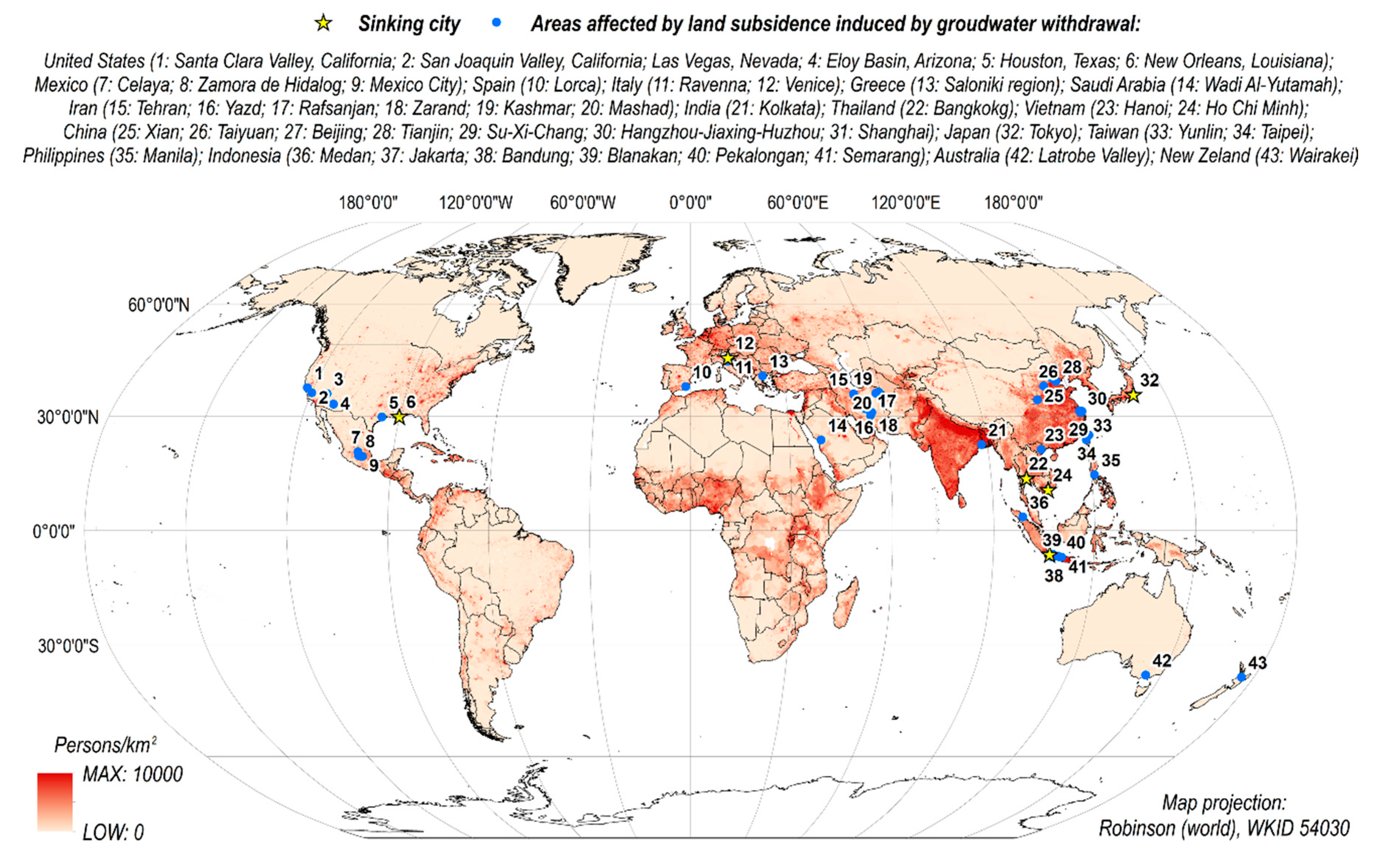
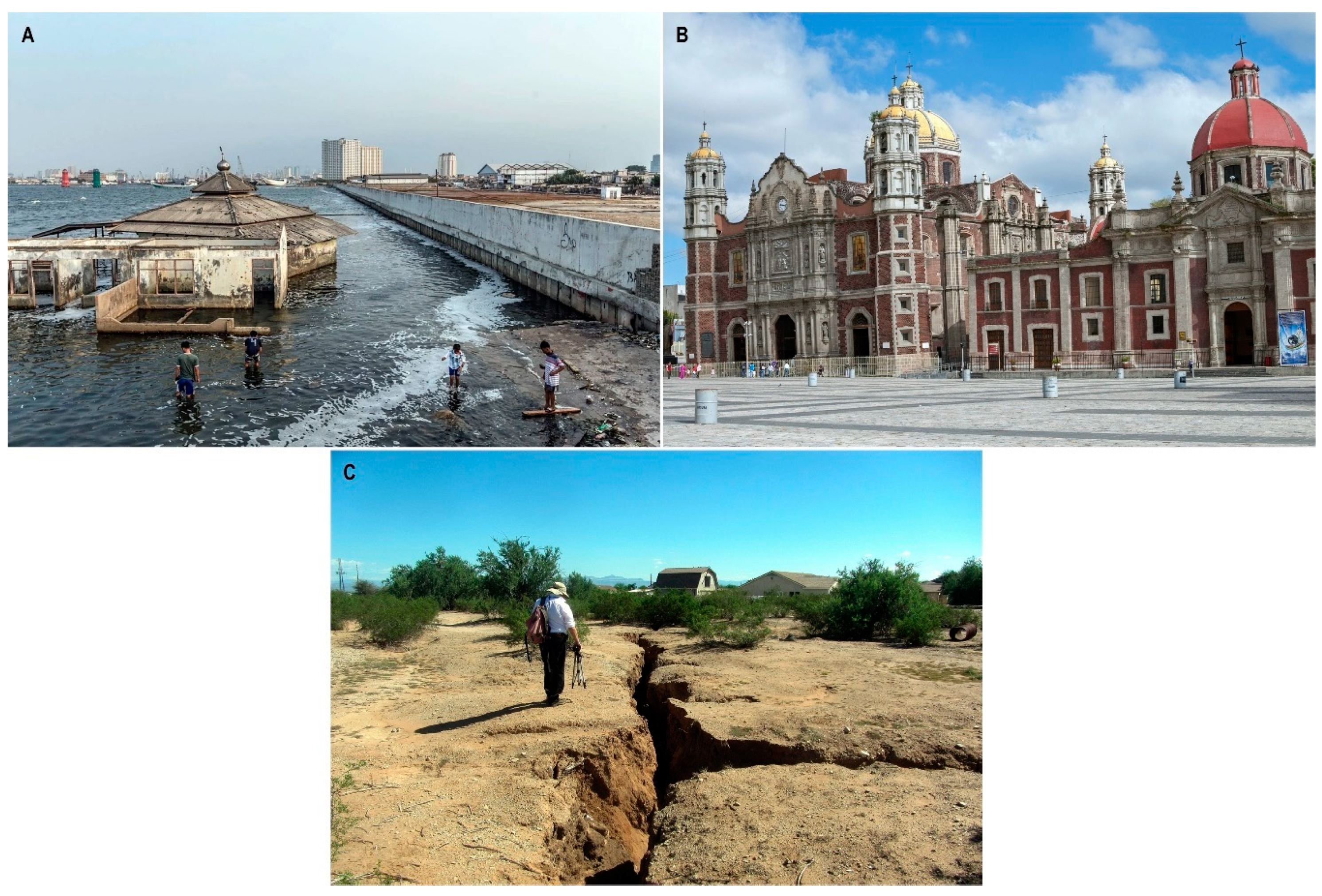
Land subsidence is one of the most common geomechanical and geotechnical consequences of pumping groundwater. The use of groundwater resources for private and industrial purposes has, in many cases, led to significant depletion, continuous deformations of the land surface and, consequently, to social and economic repercussions [33,34,35,36]. Severe aquifer system compaction due to its drainage is observed in many urban areas worldwide (Figure 1). The problem is, however, especially critical in the large coastal cities of South-East Asia. Coastal cities are usually located on the loose, unconsolidated alluvial deposits. The degree of compaction of such deposits is considerable. Given the steadily increasing average level of the world’s oceans, the coastal areas, which are affected by natural compaction due to, e.g., the consolidation process of river deltas and additional exposure to the phenomenon of drainage-induced aquifer compaction, are particularly prone to increased risk of flooding (Figure 2A; [37]). The problem of rapid and severe aquifer compaction is also present in large centres such as Los Angeles [38], Mexico (Figure 2B; [39]), New Orleans [40], Ho Chi Minh [41], Teheran [42], Bangkok [43] and Beijing [44]. Increased demand for fresh groundwater resources due to an increase in population and arable land density is also a particular challenge in desert and semi-desert areas [45]. Excessive water exploitation has led not only to a significant lowering of the groundwater head and the occurrence of drainage-induced land subsidence, but also to the inflow of saltwater into the land and thus salinization of large areas of land [46,47]. In all the cases described, the compaction of the aquifer system causes serious damage to the surface and underground infrastructure. It is estimated that the total cost of repairs for this type of damage exceeds tens of billions of Euro and, in many cases, it is impossible to make accurate estimates [8,37].

Ground surface movements resulting from rock mass drainage can range from a few centimetres to several meters [11]. The spatial extension of this phenomenon is usually extensive (even on a regional scale) and, in many cases, difficult to determine precisely. The maximum recorded value of this subsidence is 14.5 m. It is caused by the pumping of water in the geothermal field of Wairakei in New Zealand [6,50]. However, land subsidence of up to 10 m is also observed in several other parts of the world, including San Joaquin Valley, California [47] and Mexico City, Mexico [39,51]. The spatial range of the phenomenon can be extensive and can reach up to approximately 13,500 km² in the San Joaquin Valley [47]. China is currently the country with the largest cumulative area (approximately 80,000 km²) of drainage-induced land subsidence [44,52,53,54].

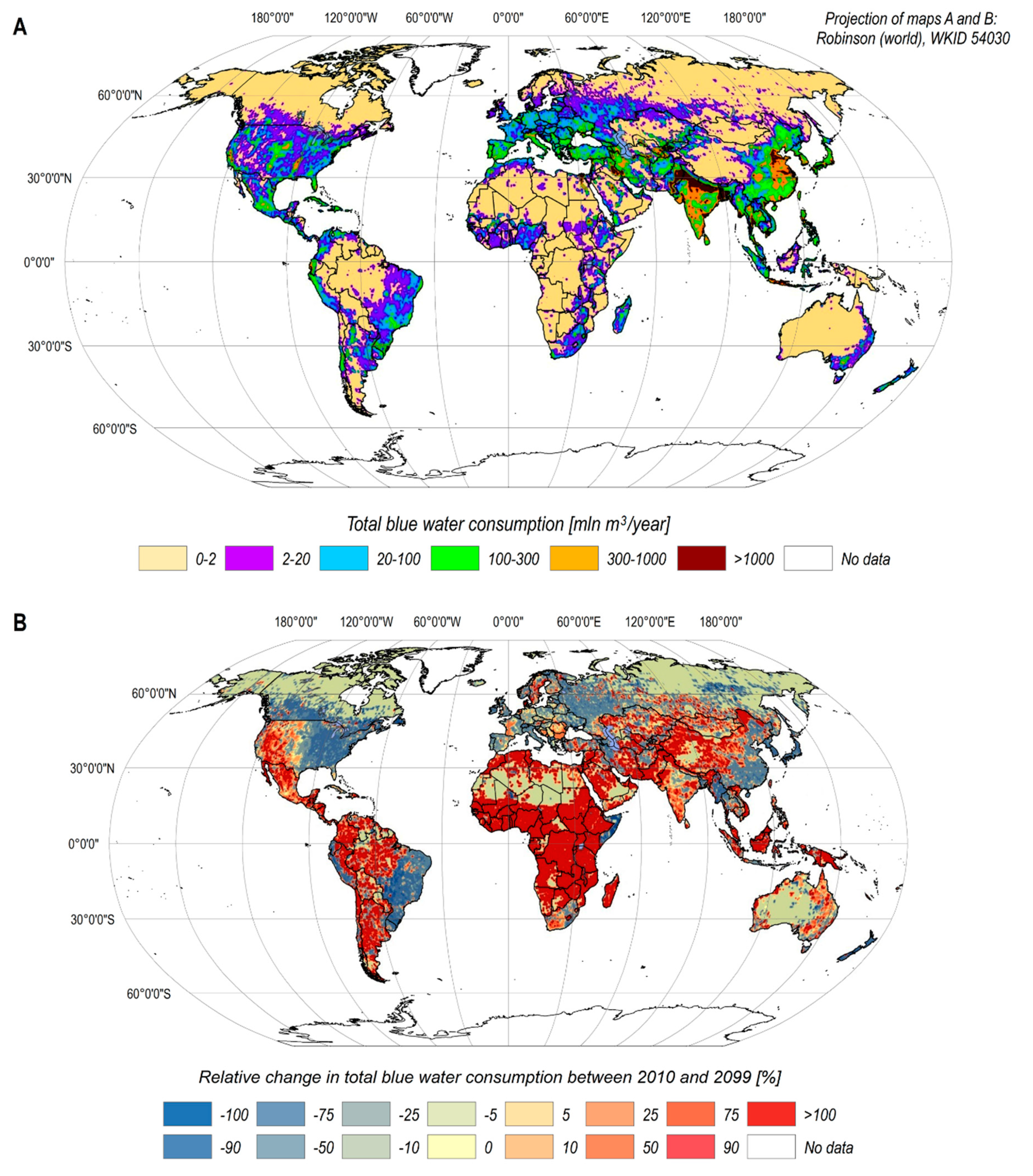
The issues related to ground surface movements induced by rock mass drainage are becoming increasingly important in terms of global climate change. Between 1960 and 2010, the estimated global consumption of groundwater increased by more than twice, and in 2010 it was approx. 2000 km³/year [36]. At present, extensive usage of water resources, including groundwater, is reported primarily in India, Pakistan, China, U.S., Mexico, Southern Europe, Northern Iran and the Nile Delta (Figure 3A). Over 90% of the world’s agricultural areas are in these places [36]. By the end of 2099, further water consumption is expected in many parts of the world. This growth will be particularly strong in central Africa, South-East Asia, the western U.S., Mexico and central South America (Figure 3B). Water consumption is increasing primarily due to rapid population growth and industrial activity in developing countries as well as climate changes, e.g., more frequent and longer drought periods. Given the above, the risk of intensification associated with the drainage-induced land subsidence is expected to increase over this century [36].

Due to the global scale of the issue, drainage induced subsidence was included in the UNESCO International Hydrological Decade Program from 1965 to 1974 [58]. The first International Land Subsidence Symposium was organized during this time. The tenth edition of this event is expected to take place in 2021 [59]. Materials prepared at these conferences include numerous scientific papers on land surface movement induced by aquifer drainage worldwide [60,61,62,63,64,65,66,67,68]. A rich source of research and an overview of examples of the studied phenomena can be also found in [11,32].

3. Geomechanics of Aquifer Response to Groundwater Withdrawal

3.1. Groundwater Depletion

As a diffuse medium, the groundwater system responds to changes in external and internal boundary fluxes (recharge and discharge) by changing its storage properties and hydraulic pressure. However, these changes have an impact on the flow of water within the aquifer. The depletion of groundwater is one of the factors most used to determine the sustainability of groundwater resources. Over-exploited aquifers are usually depleted. As a result, there is a long-term decrease in groundwater storage and hydraulic pressure in aquifers [69]. Depending on whether the environmental, economic and social consequences of groundwater depletion are acceptable or not, the use of groundwater may be considered sustainable or unbalanced [70,71].

Groundwater storage change (GWS) can be computed using changes in groundwater levels, based on Equation (1):

$$\Delta \mathrm{GWS}=\Delta \mathrm{hAS},$$

(1)

where:

$\Delta \mathrm{h}$ is the change in the hydraulic head for some specified time; $\mathrm{A}$ is the area of the aquifer representative of the head change; and $\mathrm{S}$ is the aquifer storativity.

This formula is used primarily in numerical groundwater flows to calculate cell by cell the total GWS for the model domain. However, it is usually based on inaccurate and sparsely available field data. The high heterogeneity of the aquifer system and the difficulties in estimating groundwater storage further exacerbate the GWS estimate [72]. It is crucial to examine aquifer storativity to understand psychical changes within the depleting groundwater system. Aquifer storativity is the volume of water released from storage per unit decline in hydraulic head in the aquifer, per unit area of the aquifer [73]. Storativity can be derived from the modified Equation (1) as Equation (2):

$$\mathrm{S}=\frac{\Delta \mathrm{GWS}}{\Delta \mathrm{hA}},$$

(2)

Storativity is calculated both for unconfined (Equation (3)) and confined aquifers (Equation (4)):

$$\mathrm{S}={\mathrm{S}}_{\mathrm{y}}+{\mathrm{bS}}_{\mathrm{s}},$$

(3)

$$\mathrm{S}={\mathrm{bS}}_{\mathrm{s}}=\mathrm{b}\left({\mathrm{S}}_{\mathrm{sk}}+{\mathrm{S}}_{\mathrm{sw}}\right)=\mathrm{b}\left[{\mathsf{\rho }}_{\mathrm{w}}\mathrm{g}\left(\mathsf{\alpha }+{\mathrm{n}\mathsf{\beta }}_{\mathrm{w}}\right)\right],$$

(4)

where:

${\mathrm{S}}_{\mathrm{y}}$ is the drainage porosity, also called unconfined storativity or specific yield; $\mathrm{b}$ is the aquifer thickness; ${\mathrm{S}}_{\mathrm{s}}$ is the specific storage coefficient; ${\mathrm{S}}_{\mathrm{sk}}$ is the skeletal specific storage, related to aquifer matrix compressibility $\mathsf{\alpha }$; ${\mathrm{S}}_{\mathrm{sw}}$ is the water-specific storage, related to water compressibility ${\mathsf{\beta }}_{\mathrm{w}}$; ${\mathsf{\rho }}_{\mathrm{w}}$ is the water density; $\mathrm{g}$ is the gravitational acceleration; $\mathrm{n}$ is the aquifer porosity.

Storativity is a key property of the groundwater system. It reflects the response of aquifers and aquitards to groundwater head changes. Storativity is therefore necessary to quantify the available groundwater resources. This parameter is typically obtained either in situ by measuring the decrease in the groundwater head during pumping tests or by laboratory tests of rock mass porosity. However, the applicability of storativity values determined based on pumping tests is often very limited. It stems from the applicability of such results, which are reliable only for a limited area of the aquifer near the pumping well [74]. Additionally, pumping tests are carried out mainly in the areas of potential pumping well locations. These are therefore sites with favourable hydrogeological constraints that indicate a significant amount of groundwater that can be pumped out. Simultaneously, laboratory tests are performed on small volume samples. Rock samples may be disturbed and therefore not representative of in situ conditions. Moreover, laboratory tests are usually used to estimate storativity only for a limited number of measurement points due to the high cost of performing them. The results of this work are also, in some cases, of questionable quality [75,76,77].

3.2. Aquifer Compaction

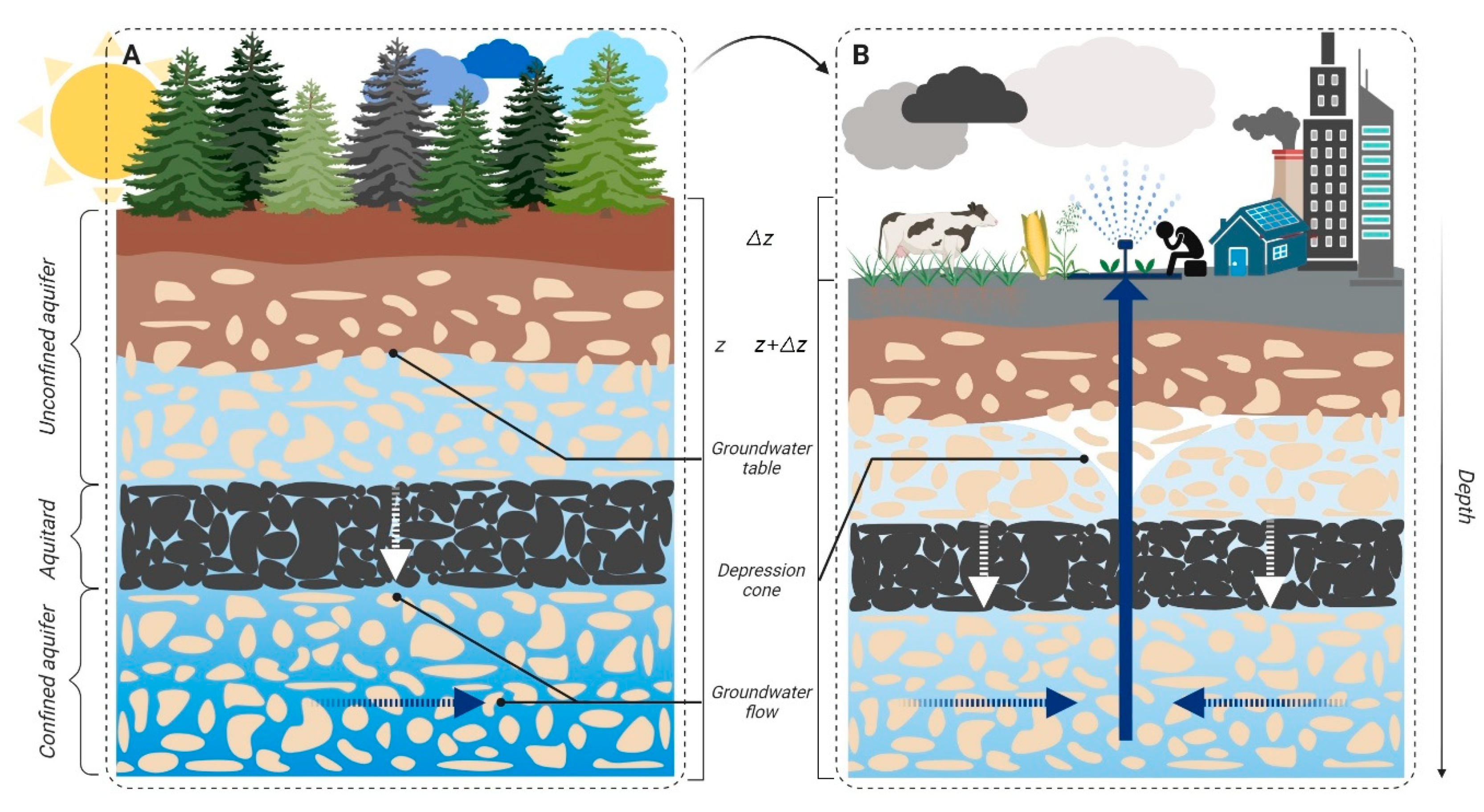
The mechanism by which the aquifer deforms as a consequence of a change in the groundwater head is well recognized. The disturbance of the natural groundwater flow system, e.g., by introducing of a well that pumps water out of this system, disrupts the hydrostatic balance of the aquifer system. It spreads in the space of this mass as a function of time, forming a cone of depression. Within a depression cone, a decrease in hydrostatic pressure is observed (Figure 4).

The increase in effective pressure is closely related to the dynamic gradient of the hydrostatic pressure. These relationships have been identified primarily through two approaches. The first approach is based on the conventional groundwater flow theory [78], and the second is based on the theory of linear poroelasticity [79]. The first approach is a specific case of the second, while the two methods are based on the principle of effective pressure [80,81]. According to this theory, under natural conditions, the total geostatic stress acting on the aquifer is balanced by the hydrostatic and effective pressure. Assuming that effective pressure remains unchanged and that the solid grains are not compressive, a variation in hydrostatic pressure implies proportional changes in the effective pressure in the aquifer, resulting in a change in the rock matrix volume. This relationship is expressed in the following Equation (5):

$${{\mathsf{\sigma }}^{\prime }}_{\mathrm{ij}}={\mathsf{\sigma }}_{\mathrm{ij}}-{\mathsf{\delta }}_{\mathrm{ij}}\mathrm{p},$$

(5)

where:

${{\mathsf{\sigma }}^{\prime }}_{\mathrm{ij}}$ are components of the effective stress; ${\mathsf{\sigma }}_{\mathrm{ij}}$ are components of total stress tensors of order two; ${\mathsf{\delta }}_{\mathrm{ij}}$ is the Kronecker delta; $\mathrm{p}$ is pore-water pressure; $\mathrm{i}$ and $\mathrm{j}$ for $\mathrm{i}=1-3$ and $\mathrm{j}=1-3$ represent the Cartesian coordinates x, y and z, respectively.

Equation (5) shows that changes in effective stress may result from changes in the total stress or changes in pore-water change pressure. The total pressure is controlled by the geostatic pressure of overlying saturated and unsaturated sediments, tectonic stresses and other factors such as topography and load history, e.g., ice mass. When the semi-permeable layers are close to the horizontal position and laterally extensive in terms of thickness, changes in hydrostatic pressure gradients in the interlayer pores are close to vertical ones. If the resulting deformations are also assumed to be close to vertical ones, the one-dimensional (1-D) form of Equation (5) becomes Equation (6):

$${{\mathsf{\sigma }}^{\prime }}_{\mathrm{zz}}={\mathsf{\sigma }}_{\mathrm{zz}}-\mathrm{p},$$

(6)

where:

${{\mathsf{\sigma }}^{\prime }}_{\mathrm{zz}}$ is the vertical effective stress; ${\mathsf{\sigma }}_{\mathrm{zz}}$ is the total stress.

If the total pressure remains constant over time, the change in effective stress is equal in magnitude and opposite to the change in hydrostatic pressure (7):

$${\Delta {\mathsf{\sigma }}^{\prime }}_{\mathrm{zz}}=-\Delta \mathrm{p},{ \mathrm{for} \Delta \mathsf{\sigma }}_{\mathrm{zz}}=0,$$

(7)

In the saturation zone, the hydraulic pressure affects the skeleton of the aquifer and the density of water stored in the rock matrix. When the hydraulic pressure increases, the skeleton volume increases, while the hydraulic pressure decreases, the skeleton volume decreases. When the hydraulic pressure is reduced, the water is released from the rock matrix. This is due to the progressive compacting of the aquifer and the expansion of the water in the rock matrix pores. Please note that ${\mathrm{S}}_{\mathrm{sk}}>>{\mathrm{S}}_{\mathrm{sw}}$ in the aquifer undergoing compaction. Assuming the values of ${\mathrm{S}}_{\mathrm{sw}}$ are negligibly small, the specific storage ${\mathrm{S}}_{\mathrm{s}}$ is practically equal to the skeletal specific storage ${\mathrm{S}}_{\mathrm{sk}}$ [32]. In addition, the development of a specific storage coefficient assumes 1-D vertical stress and strain [78,82]. Therefore, the vertical ground displacement resulting from a change in vertical stress can be expressed in terms of a change in groundwater head and defined as Equation (8):

$$\Delta \mathrm{z}\approx \mathrm{S}\Delta \mathrm{h}\approx {\mathrm{bS}}_{\mathrm{sk}}\Delta \mathrm{h},$$

(8)

where:

$\Delta z$ is the change in the vertical ground displacement.

Given the above, the relation between changes in the hydraulic head and the vertical ground displacement is used for the specific storage estimation following Equation (9) [83]:

$$\mathrm{S}\approx {\mathrm{bS}}_{\mathrm{sk}}\approx \frac{\Delta \mathrm{z}}{\Delta \mathrm{h}},$$

(9)

3.3. Groundwater System Response to Groundwater Head Changes Over Time

It is mainly the aquifer matrix compressibility that controls the land subsidence induced by the withdrawal of groundwater [18]. The 1-D skeletal compressibility $\mathsf{\alpha }$ can be defined based on the ratio of vertical strain to vertical effective stress as Equation (10):

$$\mathsf{\alpha }=\frac{\frac{\Delta \mathrm{b}}{{\mathrm{b}}_0}}{{\Delta {\mathsf{\sigma }}^{\prime }}_{\mathrm{zz}}},$$

(10)

where:

$\Delta \mathrm{b}={\mathrm{b}}_0-\mathrm{b}$ is the change in thickness of the aquifer and the primary thickness of the aquifer, respectively.

The vertical strain can also be expressed in terms of the void ratio using Equation (11):

$$\frac{\Delta \mathrm{e}}{1+{\mathrm{e}}_0},$$

(11)

where:

$\Delta \mathrm{e}=\mathrm{e}-{\mathrm{e}}_0$ is the change in void ratio, the final void ratio and the initial void ratio, respectively.

Skeletal specific storage ${\mathrm{Ss}}_{\mathrm{k}}$ in Equation (4) can therefore be expressed using Equation (12):

$${\mathrm{Ss}}_{\mathrm{k}}=\frac{{\Delta \mathrm{b}\mathsf{\rho }}_{\mathrm{w}}\mathrm{g}}{{\mathrm{b}}_0{\Delta {\mathsf{\sigma }}^{\prime }}_{\mathrm{zz}}}=\frac{-{\Delta \mathrm{e}\mathsf{\rho }}_{\mathrm{w}}\mathrm{g}}{\left(1+{\mathrm{e}}_0\right){\Delta {\mathsf{\sigma }}^{\prime }}_{\mathrm{zz}}},$$

(12)

Aquifer matrix compressibility α is conditioned by many factors. These include the distance from the drainage centre; the density and viscosity of the water as well as the permeability and porosity of the rock matrix; the vertical distribution of subsidence-prone materials; and the current stress of the rock mass and the stress curve over time. Global experience underlines that the same system of aquifers may exhibit different reactions to the deformation process according to stratigraphic characterization and the volume of groundwater pumped out [84].

Analyses and simulations of land subsidence caused by groundwater pumping are usually conducted for aquifer systems consisting of unconsolidated or poorly consolidated, coarse and fine-grained alluvial sediments (Figure 4). They consist of aquifers and semi-permeable and impermeable sediments, with thicknesses ranging from a few to several dozen metres. Under such hydrogeological conditions, the compaction of the aquifer system usually results in significant and extensive land subsidence. Semi-permeable layers cover a range of low permeable, thick and thin fine sediments. They may take the form of discontinuous interbeds in the aquifer system or may be extensive limiting units that separate individual aquifers from each other (Figure 4; [18]). Where the deeper layers of the aquifer system are compacted and have different geomechanical parameters than the loose alluvial sediments, the eligibility criterion for the individual rock layers in the aquifer system is usually the hydraulic conductivity [10]. The distinction between the rock layers that constitute the aquifer system is a necessary practice to carry out an accurate simulation of the drainage of this mass and thus determine the expected values of land subsidence. Although various methods of solving this problem require the use of different degrees of generalization of the aquifer, the division presented in Figure 4 is universal and is commonly used in many phenomenon prediction models.

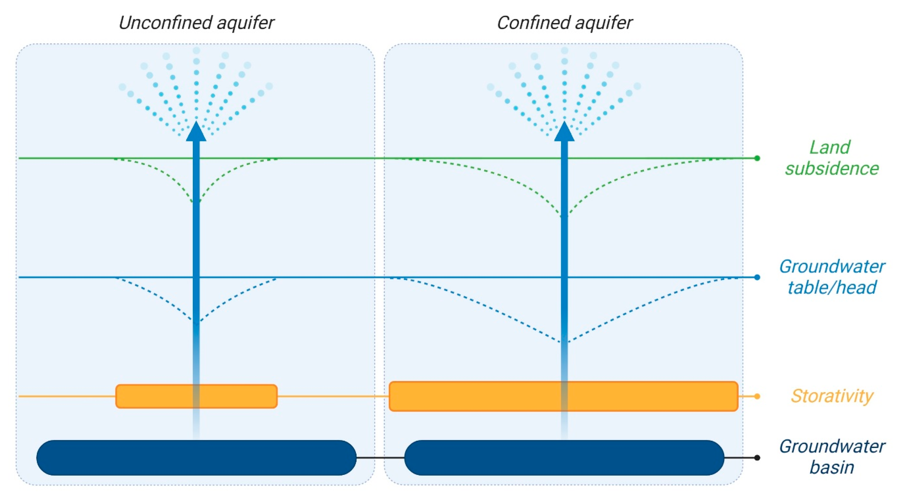
Land subsidence induced by groundwater withdrawal is characterised by various spatial distributions, depending on the hydrogeological properties of the aquifer, which is becoming depleted (Figure 5). According to the Cooper-Jacob approximation of the Theis [85], the non-balancing method for calculating the radius of influence of a steadily pumping well as the function of storativity and time in an ideal confined aquifer [86], the radius of depression cone increases with decreasing of storativity. It is, therefore, much more extensive for confined aquifers than for unconfined aquifers. The depression cone is deeper near the well pumping the groundwater out from the unconfined aquifer and wider in the case of the confined aquifer. For the unconfined aquifer, therefore, higher values of land subsidence are observed in the area of the drainage centre, whereas for the confined aquifer, land subsidence is more regionally distributed [87,88].

Vertical ground displacement may result from either elastic (recoverable) or inelastic (fixed) compaction [89,90,91], and is proportional to changes in the groundwater head and the thickness of the layer to be compacted [91]. If the groundwater head remains above the previous lowest level (stress before consolidation), elastic deformation occurs in both aquifers and semi-permeable layers [89]. In contrast, when the groundwater head falls below the previous lowest level, inelastic compaction leads to irreversible shifting of the solid grains and reduction in porosity in the groundwater system [89]. Skeletal specific storage ${\mathrm{Ss}}_{\mathrm{k}}$ can therefore be determined for both elastic (Equation (13)) and inelastic (Equation (14)) range of the strain:

$${{\mathsf{\sigma }}^{\prime }}_{\mathrm{zz}}\le {{\mathsf{\sigma }}^{\prime }}_{\mathrm{zz}}\max ,$$

(13)

$${{\mathsf{\sigma }}^{\prime }}_{\mathrm{zz}}>{{\mathsf{\sigma }}^{\prime }}_{\mathrm{zz}}\max ,$$

(14)

where:

${{\mathsf{\sigma }}^{\prime }}_{\mathrm{zz}}\max$ is the pre-consolidation vertical effective stress.

In regions experiencing mass pumping of groundwater, deformation is often inelastic. In the case of the introduction of control strategies for groundwater pumping aimed at limiting its adverse effects, a low uplift value is often observed [92,93,94,95,96,97]. In such cases, the uplift is the result of the flexible expansion of the compacted aquifer system after the recovery of the original hydrostatic pressure. This phenomenon is referred to as an elastic or poroelastic rebound [95,98]. However, since the inelastic compressibility of semi-permeable layers is 1 to 3 orders of magnitude higher than the elastic compressibility of aquifers, only a small part of the initial compaction can be recovered when water is pumped in again [89,99].

4. Simulation of Land Subsidence Due to Groundwater Withdrawal

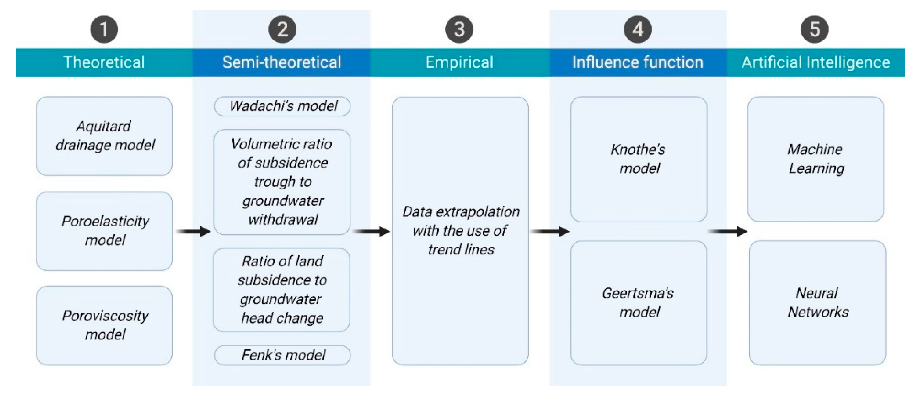
Various methods of modelling the land displacements induced by rock mass drainage can be distinguished in the literature. In 1984, Poland made one of the first attempts to classify these methods [32]. He classified the methods into three basic categories: theoretical methods (1); semi-theoretical methods (2); and empirical methods (3). Since then, this classification has also been referenced by other researchers and presented in different review articles (see Section 1). Methods (1), (2) and (3) are relatively well presented in other articles and have been used by many researchers. In this article, therefore, we focus only on describing the most important assumptions of these methods and on updating the case studies in which these methods were used. However, given the many disadvantages associated with the use of methods (1), (2) and (3), as well as the rapid development of computational algorithms based on artificial intelligence (AI), several new attempts to model land surface displacement have been identified in the literature in recent years. A distinction can be made between methods based on the function of influence and AI. Therefore, we decided that Poland’s classification would be updated and extended with two categories: methods using influence functions (4); and methods based on AI (5); (Figure 6).

4.1. Theoretical Methods

Theoretical methods provide a holistic approach to the issue of deformation of the aquifer system and land subsidence resulting from groundwater pumping. They take into account both the physical, hydrogeological and geomechanical properties of the rock matrix to be compacted and the water that flows through it. The application of these methods requires a broad recognition of the qualitative and quantitative constraints of the aquifer system under investigation such as the change in hydraulic head, the aquifer storativity, porosity and thickness, groundwater density and pore-water pressure, effective stress in the aquifer system or the change in the vertical ground displacement. This is necessary due to the significant parametrization of the prediction models. For this reason, they are difficult to implement, especially in areas with a poor understanding of the physical, hydrogeological and geomechanical properties of the rock mass.

4.1.1. Aquitard Drainage Model

It was Riley who developed the aquitard drainage model [100]. He used the quantitative theory of 1-D vertical compaction proposed by Terzaghi [80,81]. The aquitard drainage model is based on the theory of conventional groundwater flow and two principles of consolidation. The first is the principle of effective pressure (Equation (5)), the second is the principle of hydrodynamic theory, which describes the relation between hydraulic pressure, stress between the aquifer particles and water flow in the rock mass.

The standard diffusion equation for the 3-D transient groundwater flow expresses Equation (15):

$${\nabla }^2\mathrm{h}=\frac{{\partial }^2\mathrm{h}}{\partial {\mathrm{x}}^2}+\frac{{\partial }^2\mathrm{h}}{\partial {\mathrm{y}}^2}+\frac{{\partial }^2\mathrm{h}}{\partial {\mathrm{z}}^2}=\frac{\mathrm{Ss}}{\mathrm{K}}\frac{\partial \mathrm{h}}{\partial \mathrm{t}},$$

(15)

where:

$\mathrm{K}$ is the hydraulic conductivity; $\mathrm{t}$ is the time.

The aquitard drainage model is based on the assumption that the water flow in semi-permeable layers is substantially vertical when pumping aquifer systems. This assumption is justified by the high contrast of hydraulic conductivity between aquitards and aquifers. In addition, assuming a negligible value of the water-specific storage compared to the skeletal specific storage, the 1-D form of Equation (15) describes the flow of groundwater in aquitards using Equation (16):

$$\frac{{\partial }^2\mathrm{h}}{\partial {\mathrm{z}}^2}=\frac{{{\mathrm{Ss}}^{\prime }}_{\mathrm{k}}}{{{\mathrm{K}}^{\prime }}_{\mathrm{z}}}\frac{\partial \mathrm{h}}{\partial \mathrm{t}},$$

(16)

where:

′ are material properties of the aquitard; ${{\mathrm{Ss}}^{\prime }}_{\mathrm{k}}$ is the skeletal specific storage (Equation (9)), recognizing that for aquitards in unconsolidated alluvial systems ${{\mathsf{\alpha }}^{\prime }\mathsf{\beta }}_{\mathrm{w}}$; ${{\mathrm{K}}^{\prime }}_{\mathrm{z}}$ is the vertical hydraulic conductivity.

The numerical formulation of the aquitard drainage model led to the development of essential simulation tools that are now widely used on a global scale. These methods have been proposed by Helm [101,102], Witherspoon and Freeze [103], Gambolati and Freeze [104], Narasimhan and Witherspoon [105], and Neuman [106].

Helm’s [107,108] Vertical Compaction Model (COMPAC) enables the calculation of the rock mass compaction. It also allows the estimation of critical parameters of the aquifer system. This approach has been widely used in the Tucson Basin and Avra Valley, Arizona [109,110,111], as well as Taiwan [112].

Other research has focused on the possibility of calculating land subsidence in two-dimensional (2-D) and three-dimensional (3-D) groundwater flow models. Prudic [113] developed the Interbed Storage Package, version 1 (IBS-1). It was used to simulate the regional compaction of semi-permeable layers using the modular groundwater flow model MODFLOW [114]. The IBS-1 package can also be used to model the compaction of aquifers with a confined water table [115]. MODFLOW and the IBS-1 package were used to simulate 3-D regional groundwater flow and land subsidence in Avra Valley and Santa Cruz Basin, Arizona [116,117]; Antelope Valley and the Mojave Desert, California [118,119]; Houston-Galveston, Texas [120] and Saga Plain, Japan [121].

The Interbed Storage Package, version 2 (IBS-2) was developed [122] to determine the values of the semi-permeable layer compaction depending on the time of groundwater pumping. It was used to investigate the potential effects of land subsidence under conditions that delay the deformation of the aquifer system [122,123]. The SUB Package [124] IBS1 and IBS2 functionality for MODFLOW-2000 [125] and MODFLOW-2005 [126]. It was used to simulate land subsidence in Central Valley Aquifer, California [127] and Tianjin, China [128].

The packages COMPAC, IBS-1, IBS-2 and SUB used to simulate the aquitard drainage model are based on the assumption that the total geostatic pressure (Equation (7)) is constant. However, this assumption is disturbed when the groundwater head in the aquifer changes. For this reason, the results of calculations carried out based on such packages aim to overestimate the value of land subsidence.

The package originally developed as IBS-3 by Leake [123], but well-known as SUB-WT for MODFLOW-2000 and -2005 [129], allows geostatic pressure changes to be simulated as a function of the groundwater head. For this reason, it is particularly useful for simulating subsidence occurring in the unsaturated zone of the aquifer. The SUB-WT package also enables the simulation of the geostatic pressure-dependent water-specific storage. The SUB-WT package was successfully used to simulate land subsidence in Antelope Valley, California [130] and Esna, Egypt [131].

The presented packages use mainly the relationship between stress and elastoplastic deformation of the rock mass to simulate the interaction of aquifer systems. However, they do not allow modelling of the compaction of so-called “soft sediments,” i.e., clays, silt or peat, in which the process of deformation of the aquifer system runs with a viscous deformation, leading to the phenomenon of secondary compaction. For this reason, a variation of the SUB package called SUB-CR has been proposed in recent years. It allows calculations to be carried out using a visco-elastic compaction model based on the NEN-Bjerrum concept and ABC-isotach model. This package has been successfully used in modelling land subsidence in Jakarta, Indonesia [132].

A further example of using Aquitard Drainage Model is provided by Vassena et al. [133]. In the research presented, the assumptions of quasi 3-D flow (hydraulic approach) and vertical compaction were used to model land subsidence induced by the exploitation of a multi-layered aquifer in Milan, Italy. According to Gambolati and Freeze [104], a two-step quasi-stationary procedure involving a quasi 3-D hydrologic model was adopted to calculate the time-dependent hydraulic head field and a 1-D subsidence model based on these results.

4.1.2. Poroelasticity Model

The theory of poroelasticity was introduced by Biot [79]. In general, it describes the relationships between water, rock porous matrix and solid grains. As with conventional groundwater flow equations, the poroelasticity theory assumes that solid grains are not compressible [134]. In most cases, this assumption is justified by rock layer compaction studies. The compaction of solid grains is approximately 1–2 orders of magnitude less than water and approximately 2–3 rows smaller than the rock matrix. It is, therefore, relatively insignificant and generally ignored by researchers dealing with the aquifer consolidation theory.

The transient groundwater flow, including water-specific storage derived from the volume deformation of the skeletal matrix, can be expressed in Equation (17):

$$\mathrm{K}{\nabla }^2\mathrm{h}={\mathrm{Ss}}_{\mathrm{w}}\frac{\partial \mathrm{h}}{\partial \mathrm{t}}+\frac{\partial }{\partial \mathrm{t}}\nabla \cdot \mathrm{u},$$

(17)

where:

$\mathrm{u}$ is the vector representing the displacement field of the granular skeleton; $\nabla \cdot \mathrm{u}$ represents the volume strain of the skeletal matrix.

Equation (17) is one of the forms of the groundwater flow equation that expresses the volumetric deformation of the aquifer system. The complete hydromechanical solution of the volumetric strain of a rock matrix is based on a balance of forces, assuming no change in the total forces in that matrix. It is based on the coupled constitutive equations of the homogeneous medium and the deformation and displacement equations, assuming the linear elasticity and the incompressibility of the solid grains [79,135,136]. It is expressed with Equation (18):

$$\left(\mathsf{\lambda }+\mathrm{G}\right)\nabla \left(\nabla \cdot \mathrm{u}\right)+\mathrm{G}{\nabla }^2\mathrm{u}-{\mathsf{\rho }}_{\mathrm{w}}\mathrm{g}\nabla \mathrm{h}=0,$$

(18)

where:

$\mathsf{\lambda }$ is one of Lame’s constants; $\mathrm{G}$ is the rigidity or shear modulus.

Coupled Equations (17) and (18) contain a total of four equations and four uncertainties. They describe relations of poroelasticity limited by predefined assumptions. Appropriate boundary and initial conditions, specified parameter values, and numerical methods are used to approximate the partial derivatives which condition the concurrent resolution of these equations. The poroelastic model describes the combined groundwater flow processes and the deformation of aquifer systems in a more sophisticated way. Unlike the aquitard drainage model, it allows a 3-D simulation of ground surface displacements induced by the rock mass drainage [18].

The poroelastic model describes the combined groundwater flow processes and the deformation of aquifer systems in a more sophisticated way. Unlike the aquitard drainage model, it allows a 3-D simulation of ground surface displacements induced by the rock mass drainage [18].

Horizontal land surface movements accompanying the compaction of the aquifer system due to the pumping of water are usually neglected. In the past, the main reason for this was to simplify analytical calculations [78]. However, many world experiences show that groundwater pumping causes 3-D aquifer deformation [134,137,138,139]. At present, however, many researchers argue that, in the case of compressive aquifer systems, horizontal land surface movements are much smaller than vertical ones (i.e., at least 2–3 orders of magnitude smaller). They can be ignored and treated as irrelevant for this reason [23,24]. However, many of these arguments have been put forward without reasonable justification to exclude them entirely [18].

The more comprehensive application range of the aquifer system composition models, which are based on the conventional groundwater flow theory contained in the aquitard drainage model, is related primarily to the mathematical complexity of the poroelasticity model. In the historical context, it is also attributed to the lack of possibility to carry out effective monitoring of horizontal movements on a regional scale. However, due to the impossibility of simulating a full field of land subsidence displacement, the Aquitard Drainage Model has limited. The discrepancies between the aquitard drainage model and the poroelasticity model are particularly evident in the vicinity of drainage centres and where heterogeneity in aquifer systems may contribute to the displacement of land surface with significant values. Such movements may result in damage to the infrastructure. Burbey [139] has shown that, by ignoring horizontal deformation, aquifer system models based on the aquitard drainage model theory can overestimate rock mass compaction or water-specific storage values, particularly near the pumping well, where horizontal surface deformation can be significant.

Poroelastic models based on the numerical solution of Equations (12) and (13) were used in several different hydrogeological applications. Hsieh [137] used an axial-symmetrical, 2-D program called BIOT2D, which is based on the finite element method, to simulate deformations caused by changes in the groundwater head. Burbey [138] implemented the Grain Displacement Model (GDM). This applies an iterative approach to the solution of the numerical displacement field at each step until the groundwater head is reached. GDM was used to simulate land surface displacement near low permeability barriers in Las Vegas Valley, Nevada, showing that regional groundwater pumping can cause high horizontal stresses near the faults and is likely to play a crucial role in crack development and propagation [140]. Helm [141] and Li [142] showed transient horizontal movement in confined and unconfined aquifers by analytical analysis of velocity and displacement fields. They proved that pumping and injecting water into the aquifer system can result in tensile stress, which may involve cracking on the land surface along the boundary between the extensive and compressive zone of the land surface near the drainage centre. Kim [143] introduced deformation-dependent porosity and hydraulic conductivity into the theory of poroelasticity. He proved that the variable hydraulic properties of a rock medium induce its non-linear deformation. It deviates from the patterns of the deformation process, which are determined by models using time-constant hydraulic parameters. Aichi and Tokunaga [144] investigated the impact of water injection on the Kujukuri Plain aquifer system in Japan. They proved that it played a significant role in reducing land subsidence. Moreover, the authors indicated that the speed of water injection should be determined very precisely. Such action makes it possible to control the increase in hydrostatic pressure, which should be small enough not to pose a threat to the operations.

It should be noted that analytical solutions for non-linear poroelastic models were developed for rock mass compaction accompanying land subsidence induced by human-made discharge and recharge of rock mass [145,146].

4.1.3. Poroviscosity Model

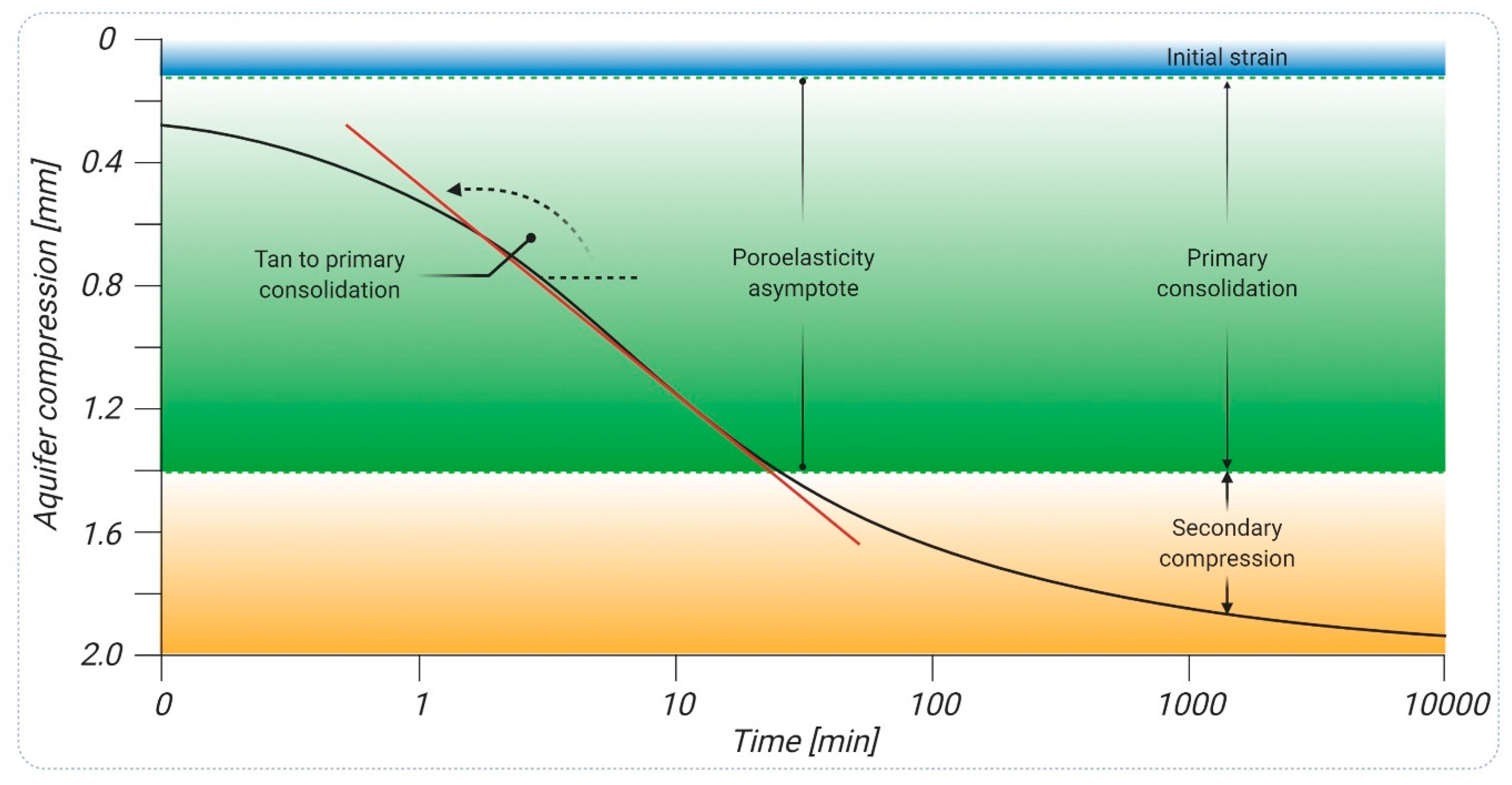
The poroviscosity theory was introduced to simulate land surface displacements to better reflect the process of deformation of argyle material due to water flowing through the saturated sediment [147]. The advantage of the poroviscosity theory over the aquitard drainage model and the poroelasticity theory is that it combines three continuous phases of preservation of the deformed material into a single time-dependent theory. The aquitard drainage model does not distinguish between these three phases of the rock mass deformation process, but in the poroelasticity theory, it must be defined as three separate physical processes that must be estimated using linear functions. The three transitional phases of the deformation process can be described as temporary deformation (1), primary consolidation (2), and secondary consolidation (3); (Figure 7). These phases can be defined based on laboratory tests for rock matrix compaction.

1-D poroviscosity the constitutive relation that describes a laterally confined material subject to axial deformation can be expressed in Equation (19):

$${\mathsf{\sigma }}^{\prime }=\mathsf{\eta }\frac{\mathrm{d}\mathsf{\epsilon }}{\mathrm{dt}}{\mathsf{\sigma }}^{\prime }=\pm \mathrm{C}\frac{\mathrm{d}\mathsf{\eta }}{\mathrm{dt}},$$

(19)

where:

$\mathsf{\eta }$ is the dynamic viscosity; $\frac{\mathrm{d}\mathsf{\epsilon }}{\mathrm{dt}}$ is the time rate of change of strain; $\mathrm{C}$ is the dimensionless poroviscous constitutive constant-coefficient; $\frac{\mathrm{d}\mathsf{\eta }}{\mathrm{dt}}$ is the time rate of the change in viscosity.

The two expressions contained in Equation (19) may be combined in the form of Equation (20):

$$\frac{\mathrm{d}{\mathsf{\sigma }}^{\prime }}{\mathrm{dt}}/{\mathsf{\sigma }}^{\prime }=\left(\frac{{\mathrm{d}}^2\mathsf{\epsilon }}{{\mathrm{dt}}^2}/\frac{\mathrm{d}\mathsf{\epsilon }}{\mathrm{dt}}\right)+\left(\frac{\mathrm{d}\mathsf{\epsilon }}{\mathrm{dt}}/\mathrm{C}\right),$$

(20)

where:

$\frac{{\mathrm{d}}^2\mathsf{\epsilon }}{{\mathrm{dt}}^2}$ is the time rate of change of $\frac{\mathrm{d}\mathsf{\epsilon }}{\mathrm{dt}}$.

Equation (20) is a non-linear expression that describes all three phases of the rock medium compaction. Only one factor in this equation, the dimensionless constitutive constant of the poroviscosity, must be defined by laboratory tests. Equation (20) may also be used to determine normal stress and mean effective stress under progressive rock mass deformation and dynamic viscosity. Darcy-Gersevenov’s law, coupled with stress balance and mass balance, is a crucial calculation tool. It combines the field of land subsidence and the average effective pressure and is expressed in Equation (21):

$$\frac{\mathrm{du}}{\mathrm{dt}}-\frac{\mathrm{K}\left(3\mathsf{\lambda }+2\mathrm{G}\right)}{3{\mathsf{\rho }}_{\mathrm{w}}\mathrm{g}}\nabla \left(\nabla \cdot \mathrm{u}\right)={\mathrm{q}}_{\mathrm{b}}+\frac{\mathrm{K}}{{\mathsf{\rho }}_{\mathrm{w}}\mathrm{g}}\nabla {\mathsf{\sigma }}_{\mathrm{m}},$$

(21)

where:

${\mathsf{\sigma }}_{\mathrm{m}}$ is the mean normal stress; ${\mathrm{q}}_{\mathrm{b}}$ is the bulk flux defined as Equation (22):

$${\mathrm{q}}_{\mathrm{b}}={\mathrm{v}}_{\mathrm{s}}-\mathrm{K}\nabla \mathrm{h},$$

(22)

where:

${\mathrm{v}}_{\mathrm{s}}$ is the velocity of solids.

The right-hand side of Equation (21) presents a forcing function that can be used to describe different types of boundary conditions. Jackson et al. [147] concluded that it is irrelevant in terms of 1-D compaction and could therefore be ignored. Based on Equations (20) and (21), a 1-D poroviscosity model was developed and implemented in the COMPAC Package [147]. The full description of the development of the 1-D and 3-D poroviscosity theory is provided by [149].

Several analytical and numerical models of 3-D land surface displacement based on the poroviscosity theory have been developed [100,150,151]. The implementation of the theory into numerical models is promising in terms of formulating a precise description of aquifers deformation process related to intensive drainage. 1-D analytical and numerical solutions enable accurate simulation of all three phases of aquifer system compaction [147].

4.2. Semi-Theoretical Methods

Semi-theoretical methods present a less complex approach to modelling dewatering-induced land displacements than theoretical solutions. These models use generalized information that describes the basic physical, hydrogeological and geomechanical parameters of the aquifer system. The calculation does not, however, take into account the complexity of the compaction process [152]. Semi-theoretical methods allow estimating the future trend of the phenomenon by using the observed relationship between the volume of pumped water/lowering of the groundwater head and the land subsidence.

4.2.1. Wadachi’s Model

Wadachi’s model was proposed in 1939 [153]. It was one of the first semi-theoretical methods of predicting land subsidence caused by drainage. The author observed the correlation of the velocity of vertical displacements, both subsidence and uplift, with changes in groundwater head in Osaka, Japan. The following Equation (23) of aquifer system compaction was proposed:

$$\Delta \mathrm{z}=\mathrm{w}\left({\mathrm{h}}_0-\mathrm{h}\right),$$

(23)

where:

$\mathrm{w}$ is the empirical constant; ${\mathrm{h}}_0$ is the critical value of the hydraulic head for which vertical ground displacement is equal to zero.

Equation (23) shows that there is a reference value for the groundwater head. Therefore, if the groundwater head $\mathrm{h}$ returns to the reference level ${\mathrm{h}}_0$, the attenuation of the vertical ground movements is observed. According to Yamaguchi’s studies, this level does not exist [153]. For this reason, the author proposed to modify Wadachi’s model. It is expressed by Equation (24):

$$\Delta \mathrm{z}={\mathrm{wz}}_{\mathrm{f}}\left[\left({\mathrm{h}}_0-\mathrm{h}\right)\mathrm{t}-\frac{\mathrm{dh}}{\mathrm{dt}}\right]\exp \left[-\mathrm{w}\left({\mathrm{h}}_0-\mathrm{h}\right)\mathrm{t}\right],$$

(24)

where:

${\mathrm{z}}_{\mathrm{f}}$ is the final land subsidence.

4.2.2. The Volumetric Ratio of Land Subsidence Trough to Groundwater Withdrawal

These methods are based on a direct comparison of the measured subsidence trough volume with the volume of water that was pumped out of the aquifer system. A specific relationship is therefore only relevant under the local conditions for which it has been defined.

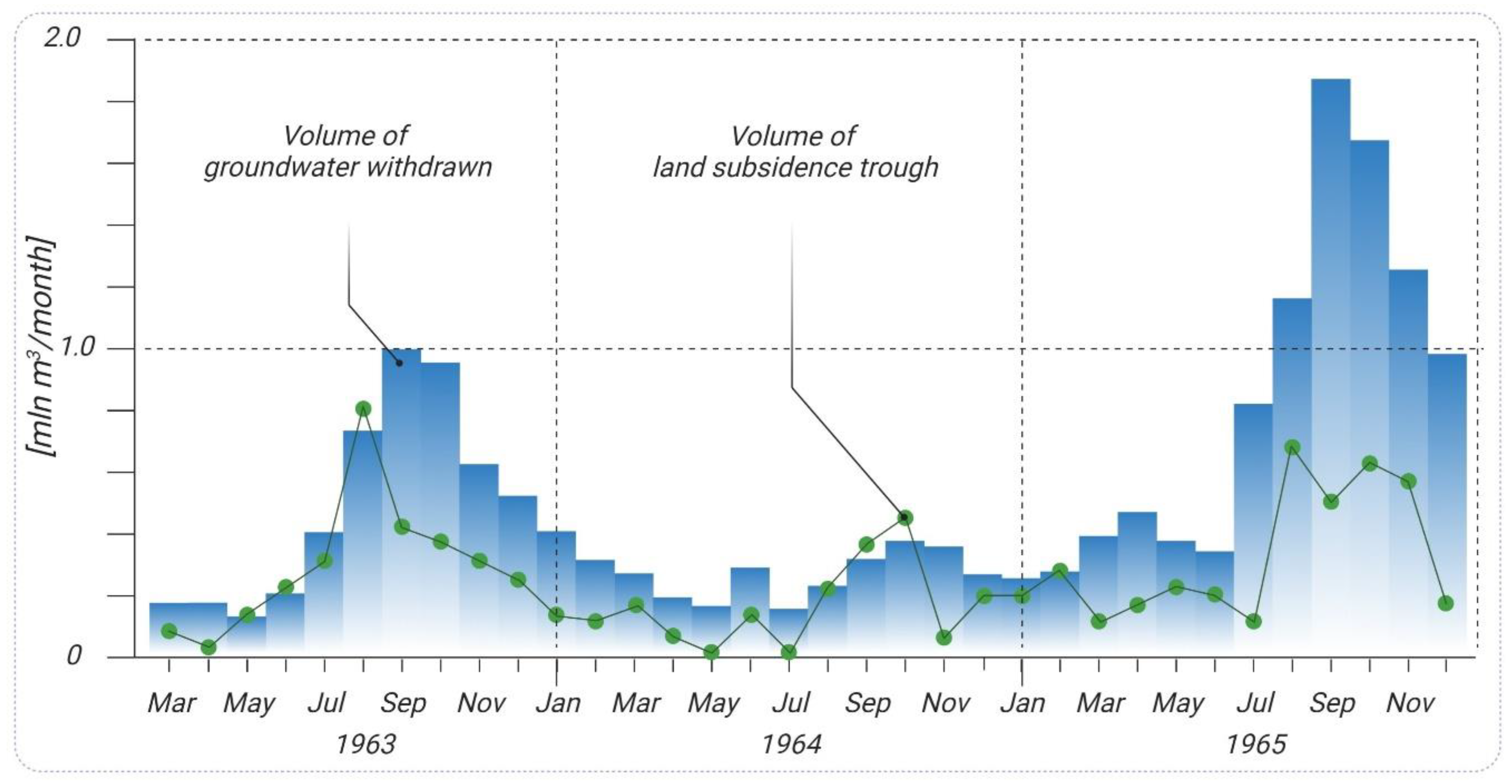
The work of Shibasaki and Shindo [154] is an example of the implementation of this method. These authors made three-year observations of the volume of water pumped out of the aquifer system in Shiroishi Plain, Kyushu, Japan and the subsidence fields in the area (Figure 8).

Based on the observed relationship, the following Equation (25) was established, which allows the volume of land subsidence to be determined:

$${\mathrm{v}}_{\mathrm{t}}=0.27{\mathrm{v}}_{\mathrm{w}}+0.25,$$

(25)

where:

${\mathrm{v}}_{\mathrm{t}}$ is the volume of the land subsidence trough; ${\mathrm{v}}_{\mathrm{w}}$ is the volume of groundwater withdrawn from the groundwater system.

4.2.3. The Ratio of Land Subsidence to Groundwater Head Change

The subsidence to groundwater head decrease represents the ratio of the land subsidence to the decrease of the groundwater head over a given period. This is therefore a change in the thickness of the aquifer system per unit of effective pressure change. The applicability of this method is useful in predicting the value of the lower limit of land subsidence in response to a surge in primary pressure that exceeds the previous maximum primary pressure value. If the hydrostatic pressure in the compacted aquifer is equal to the hydrostatic pressure in the adjacent systems, then compaction stops. For this reason, the ratio of land subsidence to groundwater head decrease can be interpreted as a measure of the compressibility of the aquifer system [32].

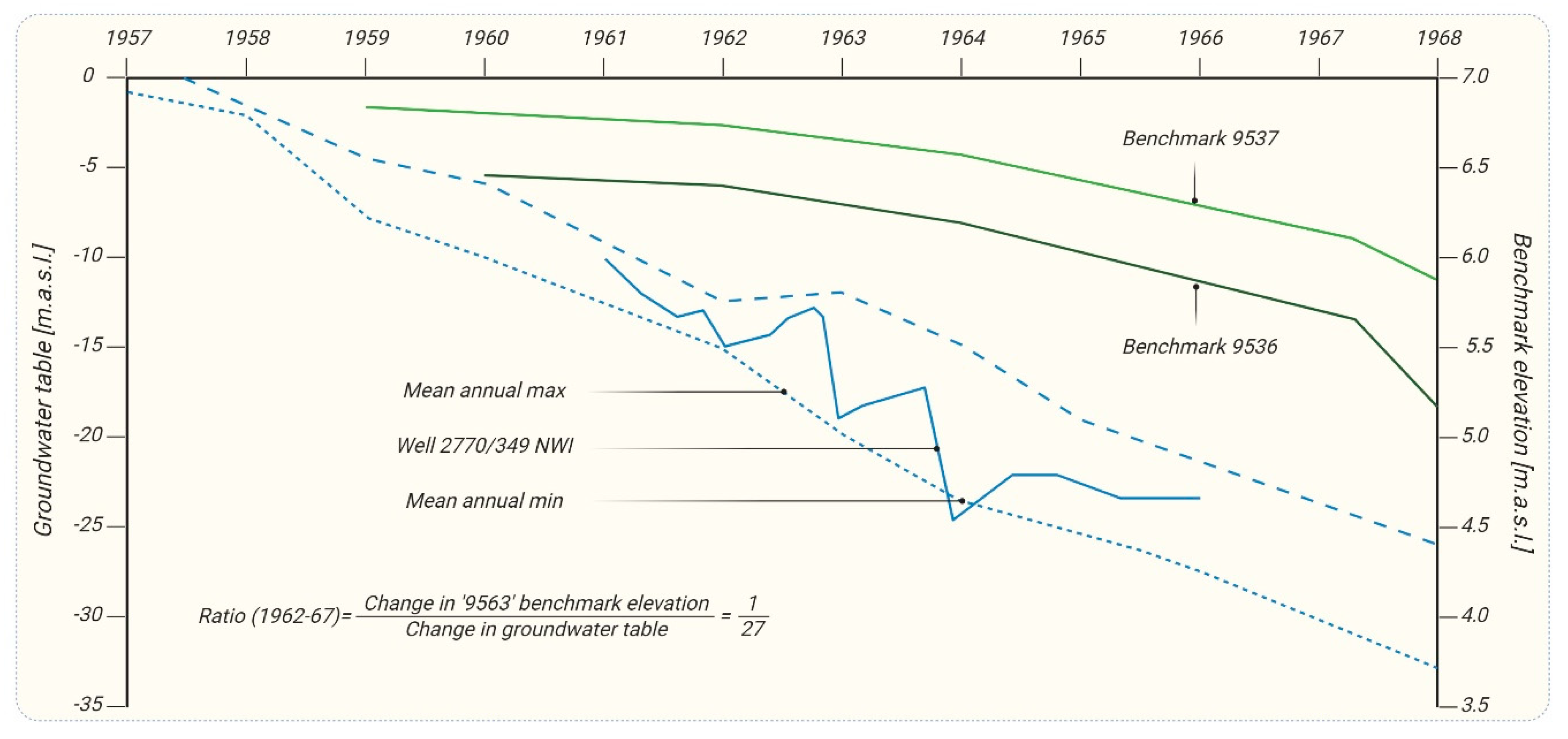
This coefficient can be obtained at discrete measurement points, for which combined observations of changes in ground vertical movements and groundwater head are made. One example of the application of this type of methodology is the research carried out in Taipei, Taiwan [155]. The value of the coefficient was 1/27 for the period 1962–1967 (Figure 9). It should be noted, however, that although the average annual trend of the minimum groundwater head in the presented case is approximately linear, the rate of land subsidence has been accelerated since 1967. As a result, the value of the coefficient of land subsidence to groundwater head decrease obtained only for the year of 1967 would be approximately 1/12. It follows that the applicability of such a method of land is limited to cases where the average value of groundwater head is representative for all aquifers in the entire study area [32].

4.2.4. Fenk’s Model

Fenk also proposed a semi-theoretical model for the forecasting of land subsidence due to the pumping of groundwater. This solution consists of comparing the relative position of the individual layers that constitute the aquifer system. It takes into account the basic geomechanical and hydrogeological properties of the medium subjected to the presented phenomenon. The basic equation of land subsidence using this method is expressed in Equation (26):

$$\Delta \mathrm{z}={\sum }_{\mathrm{i}=1}^{\mathrm{n}}\frac{{\mathrm{b}}_0}{\mathsf{\alpha }}\Delta {\mathsf{\sigma }}_{\mathrm{zz}},$$

(26)

where:

$\mathrm{i}$ for $\mathrm{i}=1-\mathrm{n}$ represents aquifers which compose the groundwater system.

One of the examples of the use of the Fenk model for the calculation of drainage-induced land subsidence is the study carried out in Saxony, Germany [156].

4.3. Empirical Methods

Empirical methods are the most basic solutions to predict the presented phenomenon. They use the information on the current status of land surface deformations to predict such phenomena in the short term. These methods do not take into account the physical, hydrogeological and geo-mechanical properties of rock and water mass. They therefore allow only an approximate determination of the value and spatial extent of the drainage-induced land subsidence in the short term [10].

Linear or non-linear data extrapolation is one of the most frequently used empirical methods. It involves embedding the function in empirical data, e.g., using the least squared method. The following functions are used: square, exponential and logarithmic. These are expressed in the respective Equations (27)–(30):

$$\Delta \mathrm{z}=\mathrm{ax}+\mathrm{c},$$

(27)

$$\Delta \mathrm{z}={\mathrm{ax}}^2+\mathrm{cx}+\mathrm{d},$$

(28)

$$\Delta \mathrm{z}={\mathrm{ax}}^{\mathrm{c}},$$

(29)

$$\log \Delta \mathrm{z}=\log \mathrm{a}+\mathrm{c}\log \mathrm{x}$$

(30)

where:

$\mathrm{a}, \mathrm{c}, \mathrm{d}$ are the equation constants.

Empirical approaches to land subsidence prediction have been used in the area of hydrocarbon extraction in the Groningen gas field in the Netherlands [157]. A rather simple parametric spatio-temporal trend model has been used to approximate the subsidence bowl at the centimetre level to exploit the smooth and gradual decay over deep gas reservoirs. Further research has been carried out on in the Bogdanka hard coal mine, Poland [158]. The authors analysed the spatio-temporal distribution of depression and land subsidence. In addition, based on the results of observations of water tables in aquifers, land subsidence and geomechanical characteristics of the rock mass, trend lines of logarithmic functions have been estimated. Subsequently, based on logarithmic functions, predictions of water table fluctuations and land subsidence were made in the entire hard coal mining area.

4.4. Influence Function Methods

The group of methods based on the theory of influence function includes concepts that are commonly used by the mining industry to predict land subsidence caused by the operation of underground mines [159]. The analysis and simulation of such subsidence involve the assessment of factors that are often quite complex and difficult to interpret and classify. Theoretical and semi-theoretical methods present limitations for the comprehensive identification of geological variability and the use of measurement data describing the deformation of the rock matrix over time.

The methods presented assume that the primary cause, which is the deformed rock mass, results in an elementary impact on the land surface. A generalized input parameter for the observable and measurable effects of underground deposit extraction, e.g., water pumping, is assigned to each of the spatial elements subject to discretion. Models based on influence function use a limited number of parameters, each of which has a physical interpretation and can be seen as a compromise with theoretical models [160,161]. These methods can therefore potentially serve as a comprehensive tool, especially when describing phenomena that require a significant degree of parameterization. Many studies have shown that the application of influence function-based methods might indicate similar accuracy in predicting land subsidence as the results of numerical modelling based on the most commonly used theoretical models [162].

4.4.1. Knothe’s Model

This model is based on the division of the rock matrix prone to compaction into elementary reservoir elements. The proposed assumption allows reservoir elements to be used in the form of cuboids with arbitrarily shaped bases [163]. Based on such a solution, the computational applicability of the method increases. According to the Knothe model, land subsidence is the result of the compaction of the porous rock matrix and may be expressed with Equation (31):

$$\Delta \mathrm{z}={\mathrm{C}}_{\mathrm{m}}{\Delta \mathrm{pb}}_0{\iint }_{\mathrm{L}}\frac{1}{{\mathrm{r}}^2}\exp \left(-\mathsf{\pi }\frac{{\mathrm{R}}^2}{{\mathrm{r}}^2}\right),$$

(31)

where:

$\Delta \mathrm{p}={\mathrm{p}}_0-\mathrm{p}\left(\mathrm{t}\right)$ is the change in the pore-water pressure and the initial pore-water pressure, respectively; $\mathrm{L}$ is the geometry of the reservoir element; $\mathrm{R}={\left[{\left(\mathrm{x}-{\mathrm{x}}_{\mathrm{s}}\right)}^2+{\left(\mathrm{y}-{\mathrm{y}}_{\mathrm{s}}\right)}^2\right]}^{\frac{1}{2}}$ is the distance in the horizontal plane between a location of a reservoir element $\mathrm{x}, \mathrm{y}$ in the rock matrix and a calculation point on the terrain surface ${\mathrm{x}}_{\mathrm{s}},{ \mathrm{y}}_{\mathrm{s}}$; ${\mathrm{C}}_{\mathrm{m}}$ is the 1-D compaction coefficient, which can be defined as Equation (32):

$${\mathrm{C}}_{\mathrm{m}}=\frac{\Delta \mathrm{b}}{\mathrm{b}\Delta \mathrm{p}},$$

(32)

and $\mathrm{r}$ is the radius of influence defined as Equation (33):

$$\mathrm{r}=\frac{\mathrm{H}}{\mathrm{tg}\mathsf{\beta }},$$

(33)

where:

$\mathrm{H}$ is the mining depth; $\mathrm{tg}\mathsf{\beta }$ is the parameter corresponding to the strength properties of the rock mass.

The Knothe method is classified to the groups of stochastic methods [164,165,166]. Models of this type first appeared in applied research many years ago. However, they are widely recognized today and more and more often used due to their relatively small number of parameters and high reliability of calculations. Nevertheless, like all predictive models, the Knothe method requires the definition of parameters that control the calculation process. Both ${\mathrm{C}}_{\mathrm{m}}$ and $\mathrm{tg}\mathsf{\beta }$ coefficients make up the set of basic parameters of the model. Their values should correspond to the local conditions in the rock mass [167,168]. For this reason, the determination of these parameters is an essential requirement for the reliable modelling of ground surface movements. Many researchers emphasize that assessment of model parameters mode is critical for the accuracy and reliability of forecasts [167,169,170,171,172]. Frequently, however, the values of these parameters cannot be obtained directly from in situ tests; in other cases, the density of samples is insufficient [173]. In such a situation, the presented model requires the use of dedicated parameterization methods and a unique computational approach [174].

Truplett’s studies are one example of the Knothe method used to predict land subsidence due to pumping water from underground reservoirs [175]. He used the method presented to assess subsidence produced by groundwater withdrawal in California, USA. Moreover, Witkowski used the Knothe method to simulate groundwater-induced land subsidence in the Bogdanka hard coal mine in Poland [174]. Other examples include the forecast for rock mass deformation caused by pumping fluidized bed deposits, including crude oil and natural gas [176,177].

4.4.2. Geertsma’s Model

McCann and Wilts initially proposed the method of forecasting land subsidence in the porous rock matrix based on the tensor centre [178]. It shows considerable similarity to the model proposed by Geertsma and known in the literature as the strain nuclei [179]. The application of both theories is based on the elasticity theory. Therefore, it involves the assignment of linear elastic properties to both disturbed rock mass and surrounding rock and soil. Additionally, the elastic constants inside and outside the disturbed rock mass are assumed to be identical, which is probably not correct, but is justifiable for a rough estimation of the surface uplift. The land subsidence, according to Geertsma’s model, is expressed by Equation (34):

$$\mathrm{s}=-\frac{1-\vartheta }{\pi }{\int }_{\mathrm{M}}{\mathrm{C}}_{\mathrm{m}}\frac{\mathrm{H}}{{\left({\mathrm{R}}^2+{\mathrm{H}}^2\right)}^{\frac{3}{2}}}\Delta \mathrm{p}\Delta \mathrm{M},$$

(34)

where:

$\vartheta$ is the Poisson’s ratio; $\mathrm{M}$ is the centre of a circular zone of disturbed rock by the groundwater exploitation over which the land subsidence occurs.

At first, the concept of Geerstma’s model was created for modelling land subsidence above the Groningen reservoir [163]. However, the model was subsequently enhanced by Gambolati [180], who extended Geertsma’s homogenous model to the heterogeneous tension centre model. Nevertheless, both the Geertsma’s and the Gambolati’s model do not vary a lot. Moreover, the similarities between the models are discussed in [163,181]. The prediction of vertical ground movements based on the nuclei strain concept was carried out by Bekendam and Pöttgens [182]. They applied Geertsma’s model to assess the impact of flooding of the Limburg mine on the land uplift and sinkholes formation.

4.5. AI Methods

In recent years, there has been a growing interest in using AI methods to model phenomena that require a much higher level of parametrization. The main advantage of using AI-based methods is their ability to identify complex relationships between individual data sets and to find and examine hidden features in the data itself. Such action is not possible by using traditional prediction methods based on empirical, semi-theoretical, theoretical and impact function models, nor by implementing advanced numerical solutions to these models. The reliability of modelling and predicting land surface movements using traditional prediction methods depends on the availability of non-small measurement data. These models are therefore particularly challenging to implement and often provide unreliable results for regional and global studies.

AI methods are applied for the identification and classification of patterns, for the prediction of time-series and statistical analysis of data and the detection of unknown data regularities, for the formulation of decision-making rules, as well as for the modification, generalization and precise clarification of data. A description of the mathematical formulation of these solutions is omitted in the paper due to the multitude of techniques presented above and the considerable diversity of adaptation possibilities of particular solutions to solve specific research problems. Nevertheless, a comprehensive source of knowledge of this subject can be found in numerous studies [183,184].

One of the areas in which AI has found widespread use in recent years is the determination of the susceptibility of the area to land subsidence. The Land Subsidence Susceptibility Map (LSSM) identifies areas that are subject to land subsidence. In short, it is defined as the probability of land subsidence occurring at a given location. Susceptibility thus refers to the spatial likelihood or probability (given in either qualitative or quantitative terms) that land subsidence will occur in the future. The LSSM takes into account where land subsidence occurs and what causes it. Essentially, a successful land subsidence study is associated with considering the integration of several environmental factors [185]. The geo-database in land subsidence modelling must therefore cover different types of thematic information. InSAR and GIS data are useful tools for integrating the development of land subsidence studies [51,186]. The following factors are mainly considered for the production of the LSSM: volume of groundwater withdrawn, slope, aspect, lithology, distance from the fault, distance from the river, type of aquifer, land use and cover [187]. According to the literature review, several models and methods (qualitative and quantitative) have been successfully applied and developed in different parts of the world for land subsidence susceptibility mapping. AI methods successfully implemented to determine the susceptibility of a given area to land subsidence include Logistic Regression (LR) [188], Frequency Ratio (FR) [189], Analytical Hierarchy Processes (AHP) [190], Weight-of-Evidence (WOE) [191], Evidential-Belief-Functions (EBF) [189], Grey Model (GM) [192], Sensitivity Analysis (SA) [193], Fuzzy Logic (FL) [194], Adaptive Neuro-Fuzzy Inference System (ANFIS) [195], Artificial Neural Network (ANN) [185], and Support Vector Machine (SVM) [196].

To date, only a few studies have been conducted to develop new methods for predicting land subsidence induced by a rock matrix dewatering using AI. Witkowski and Hejmanowski [197] applied a multilayer perceptron network and the method of supporting vectors for the analysis and simulation of a large-area subsidence trough in the area of one of the underground mines in Poland. The authors obtained satisfactory simulation results, indicating at the same time the need to use empirical data to validate the modelling outcomes. Zamanirad et al. [198] used boosted regression trees (BRTs), generalized additive model (GAM) and random forest (RF), together with anthropogenic and environmental predicators, to predict land subsidence in southern Iran. These predictors were generated based on extensive field studies. The research carried out shows that the main factors causing land subsidence are as follows: groundwater pumping, lithology, distance from surface water streams and height of the studied area above the assumed reference level. Zhu et al. [199] examined the spatial relationships between land subsidence and the three factors they considered crucial in terms of the formation of dewatering-induced deformations of the aquifer system. These included: groundwater head, the thickness of compressible aquifers and distribution of built-up areas. Based on the spatial analysis of land subsidence and the three presented factors, a significant non-linear relationship was found between them. Based on the backpropagation algorithm (BPN), which was combined with the genetic algorithm (GA), the results of these analyses were successfully applied to simulate the regional spatial distribution of land subsidence.

5. InSAR as a Supportive Tool for Groundwater Withdrawal-Related Subsidence Prediction Models

InSAR is one of the most commonly used technologies for measuring ground surface displacement. Many of the satellites acquired radar images starting from 1992 onwards.

SAR satellites that have been most used for InSAR studies in land subsidence research are as follows: ERS [200], Radarsat [201], ENVISAT [200], COSMO-SkyMed [202] and TerraSAR-X [203]. The radar images acquired during these missions were characterized by various spatio-temporal resolutions. These values were, e.g., up to 35 days for ERS and ENVISAT missions and up to 30 m for ENVISAT missions, respectively [200]. Noticeably, ERS and ENVISAT data are freely accessible to all users, whereas COSMO-SkyMed and TerraSAR-X data can be obtained for free for science through Announcements of Opportunity since 2015 and 2013, respectively. Nevertheless, it is the Open Source Data Sharing Policy of the Sentinel-1 mission of the European Space Agency that has greatly increased the accessibility to satellite radar images for all users worldwide. Sentinel 1-A and 1-B satellites have been operating together since 2016 and perform a 6-day cycle of radar imagery at a spatial resolution of 5 × 20 m [31]. The processing of such large data sets is now becoming easier due to the rapid development of advanced computational algorithms and even the partial automation of operation on external servers (cloud computing) [30,204,205,206]. This allows users to save time and disk space needed to perform complex calculations [204,205]. There is now a large InSAR image archive in most parts of the world, covering almost 30 years. Given such a long-time horizon and the considerable processing capacity of InSAR data, this ground monitoring technology contributes to significant progress in determining the spatio-temporal distribution of land displacements almost on a global scale.

The latest developments in space-borne SAR sensors, seen in the recent Sentinel mission, provide an ever-improving signal/noise ratio, enabling the following: a higher repeat pass frequency, enabling, for instance, to infer short-term variations, e.g., monthly, with high temporal detail, and relate them to seasonal recharge and discharge patterns; and increased spatial coverage.

The first InSAR application dates back to the late 1980s [207], when Differential Radar Satellite Interferometry (DInSAR) was used. The DInSAR method uses phase difference between two registered radar images acquired over the same area at different times [208]. The difference in phase is calculated as an interferogram. Ideally, each interferogram should contain only a difference in the phase associated with the displacement of the land surface. The differences in phases may also arise from external factors that are not related to the displacement of the land surface. Phase ${\Delta \mathsf{\phi }}_{\mathrm{int}}$ is therefore complex and is usually expressed as the sum of the five main components (Equation (35); [209]):

$${\Delta \mathsf{\phi }}_{\mathrm{int}}={\mathsf{\phi }}_{\mathrm{displ}}+{\mathsf{\phi }}_{\mathrm{topo}}+{\mathsf{\phi }}_{\mathrm{atm}}+{\mathsf{\phi }}_{\mathrm{orb}}+{\mathsf{\phi }}_{\mathrm{noise}}+2\mathrm{k}\mathsf{\pi },$$

(35)

where:

${\mathsf{\phi }}_{\mathrm{displ}}$ is the displacement phase component; ${\mathsf{\phi }}_{\mathrm{topo}}$ is the topographic phase component; ${\mathsf{\phi }}_{\mathrm{atm}}$ is the atmospheric phase component; ${\mathsf{\phi }}_{\mathrm{orb}}$ is the phase component due to the orbital errors; ${\mathsf{\phi }}_{\mathrm{noise}}$ is the noise; $\mathrm{k}$ is an integer value called phase ambiguity.

The ultimate purpose of InSAR data processing is to estimate the phase related to the ground motion. This task is performed by completely removing or reducing as much as possible the remaining components of the signal. Additionally, given the wrapped nature of the phase signal (2π function), it is necessary to use algorithms to reconstruct the full radar waveform phase image [209]. With this in mind, the main constraints for DInSAR are temporal and geometric de-correlation, which strengthens the noise component [209], the errors of developing the radar wave phase [210] and incorrect estimation of the atmospheric component [211].

To reduce these constraints, interferogram processing techniques based on time series (MTInSAR) have been developed. MTInSAR methods use a stack of differential interferograms which are linked together by a common master image [212]. This approach allows for a correct estimation of all components of signal phase noise to limit them (one cannot remove them entirely). Therefore, it is possible to calculate the component of the actual displacement with higher precision.

Over the last two decades, many different algorithms for processing SAR data based on time series have been developed. The first of these was proposed at the beginning of the 21st century as the Persistent Scatterer Interferometer (PSInSAR, [213]). Several more MTInSAR techniques were presented in the following years. These include Small Baseline Subset (SBAS, [214]), Coherent Pixel Technique (CPT, [215]), Interferometric Point Target Analysis (IPTA, [216]) and SqueeSAR [26]. In light of these examples, many other research groups have focused their efforts on implementing new specific MTInSAR techniques. For a broader review of these algorithms as well as InSAR principles, please refer to [25,217].

5.1. Application of InSAR Data in Groundwater Withdrawal-Related Subsidence Issues

To manage groundwater and to prevent or reduce land subsidence, it is essential to have an aquifer deformation model that makes it possible to predict the land subsidence that will occur due to changes in the groundwater system. The starting point for the development of a deformation model, at any location, is the availability of land surface displacement rates that could be nowadays achieved primarily with the use of InSAR. The most significant parameters used in modelling approaches (see Section 4) can be derived from InSAR data to improve groundwater models. This can be done by the proper processing and interpretation of such information. The solution therefore allows the groundwater manager to consider different scenarios that result in changes in the groundwater head, and then to use the predicted changes to determine the corresponding subsidence rates.

InSAR is increasingly used in hydrogeology due to its high accuracy in measuring ground surface displacement, wide-area coverage and cost-effectiveness. The use of InSAR in hydrogeological research allows for a much broader approach to water hazard assessment. The rapid development of this measurement technology over the last dozen years has improved the possibilities of mapping, monitoring and simulation of groundwater flow in the compacted aquifer system [11]. Quantitative observations of land surface displacements and estimates of hydrogeological parameters obtained from InSAR data are very useful in constructing regional hydrogeological models of groundwater flow and land surface displacements [11,218]. Many studies carried out over the last three decades have indicated that surface displacement associated with the deformation of the aquifer system are not only common, but can also be reliably measured and described in spatio-temporal terms [4,11,18,83,94,118,218,219].

Due to the considerable amount of research conducted on the use of InSAR in hydrogeological studies, in the following part of the article, only the most crucial examples are presented [218]. These aim at determining the following:

• structural boundaries of aquifer systems (e.g., tectonic faults);
• the spatio-temporal distribution of land surface displacements and hydrogeological heterogeneity of aquifer system;
• values of storage coefficients and hydraulic conductivity of the aquifer system.

5.1.1. Structural Limits of the Aquifer

Boundaries of groundwater flow models are often determined based on faults [73]. Tectonic dislocations may be important hydraulic elements for regional groundwater systems. They usually play the role of large hydraulic barriers that disrupt aquifer continuity and may alter groundwater flow paths. Therefore, faults may act as a boundary between hydrogeological units with contrasting hydraulic conductivity. Additionally, hydrogeological barriers characterised by low hydraulic conductivity may induce steep hydraulic gradients. For this reason, fault detection is usually based on a regional potentiometric surface map analysis. However, a reliable analysis of the groundwater head requires a significant degree of recognition of the aquifer system. This type of measurement is not consistent in many areas. For this reason, they provide only fragmentary knowledge of the hydrogeological characteristics of the area under study [73].

InSAR enables the acquisition of a spatially and temporally detailed land surface displacement field. The detection of discreet, differential displacements of the terrain surface is possible with the use of the A-DInSAR technique. Employing a thorough interpretation of the results of such measurements (supported by external data, e.g., seismic information), it is possible to identify unrecognized faults or to update their known location. The efficacy of InSAR in the identification of potential fault locations depends on the compressibility of the rock skeleton and the temporal changes of the groundwater head in adjacent hydrogeological units, which may be separated by the fault. This is because the presence of the fault can therefore be defined by steep displacement gradients of the surface, which typically take linear direction. A significant land surface movement gradient is also favoured by changes in the groundwater head on one side of the fault.

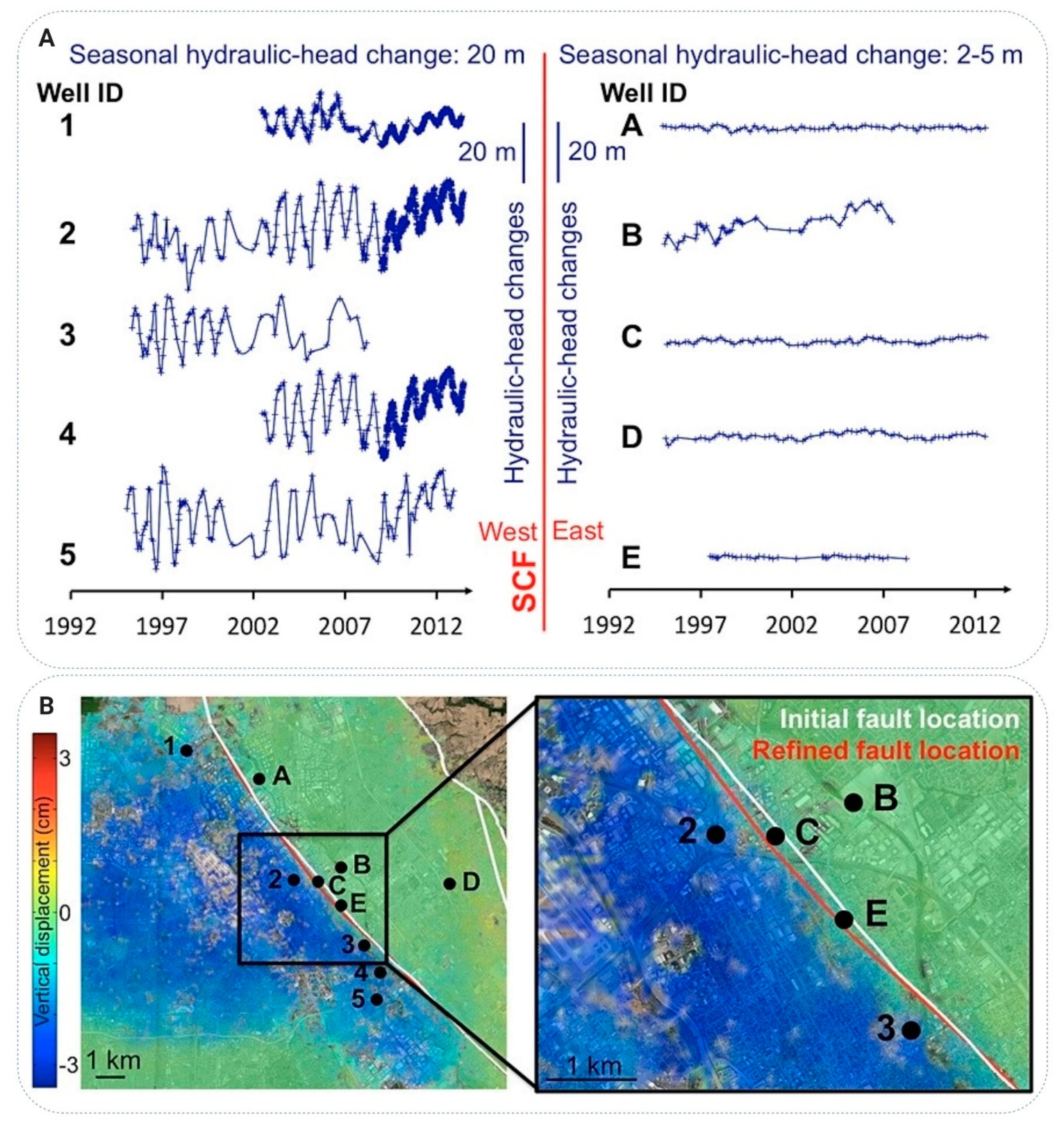
One example of how detailed maps of land surface displacements obtained from InSAR contribute to the identification of new information on the role of faults in aquifers is the research conducted in the Santa Clara Valley (SCV), California [98]. Due to the lack of marked surface changes, which could indicate the occurrence of a fault in the analysed region, its location was determined based on seismic and InSAR imaging [51,94]. A detailed analysis of the seasonal distribution of surface displacements, coupled with changes in the groundwater head on both sides of the fault, was assumed by the fault detection methodology carried out with the use of InSAR (Figure 10). Based on the research, it was found that the fault contributes to water flow disturbances on a regional scale, constituting an area with reduced specific storage and aquifer compaction.

Many other studies indicate that InSAR enables the presence of unrecognized faults to be recorded as barriers to groundwater flow in aquifers [92,93,94,95,96,220,221,222,223,224,225,226] In addition, the hydrogeological constraints of the fault zone may be estimated based on InSAR data [140,227].

5.1.2. Spatio-Temporal Distribution of Land Subsidence and Heterogeneity of Groundwater System

Areas affected by land surface displacements require effective methods of identification. The monitoring of this phenomena makes it possible to determine the spatio-temporal distribution of aquifer system deformations and thereby to identify the mechanism of the investigated process. In the past, the use of InSAR in monitoring was mainly concerned with a quantitative analysis of the distribution of land surface displacements over a large area. These analyses therefore allowed a limited study of the spatial heterogeneity of the groundwater system only. However, the major improvement in such studies is provided by A-DInSAR techniques [24,44,200,228,229,230].

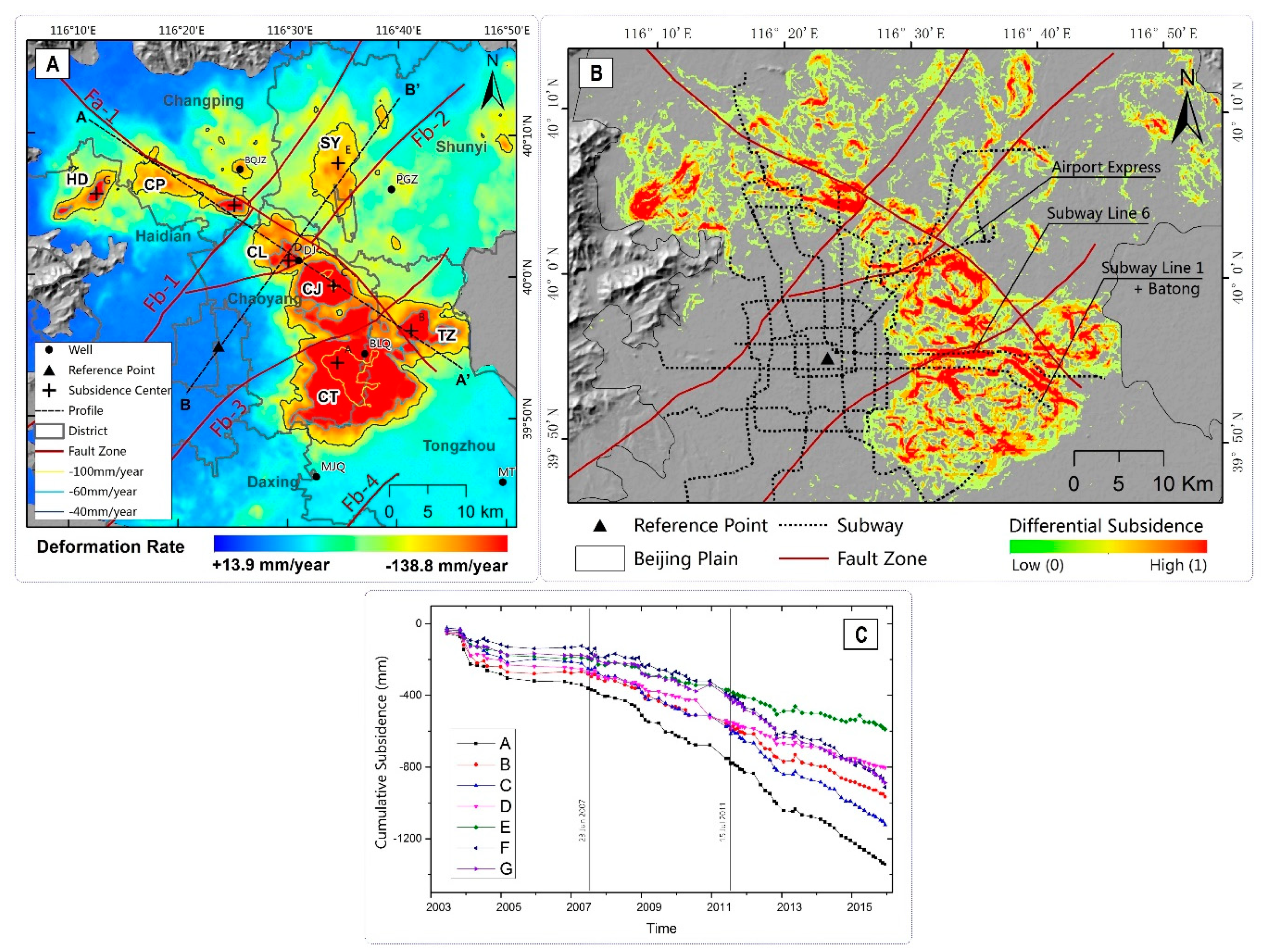
PSInSAR has been used to detect and analyse the long-term spatio-temporal evolution of land subsidence in the period 2003–2015 in Beijing, China [231]. In this study, ENVISAT, Radarsat-2 and TerraSAR-X radar images were used, while independent levelling measurements confirmed the high accuracy of the InSAR results. The mean deformation rate map was produced from PS points time-series data during the study period (Figure 11A). Areas of differential subsidence were mostly located at the boundaries of the seven subsidence bowls, as indicated by the subsidence rate slope (Figure 11B. The radar-based deformation velocity ranged from −136.9 to +15.2 mm/year during 2003–2010, and −149.4 to +8.9 mm/year during 2011–2015 relative to the reference point (Figure 11A,C). Notably, the area of greatest subsidence was generally consistent with the patterns of groundwater decline in the Beijing Plain.

Strong data processing capacity approaches focused on A-DInSAR techniques benefit from the ability to identify land surface displacements with detailed geomechanical characterisation. These include linear and non-linear deformations as well as seasonal variations, e.g., as a result of seasons or changes in the volume of water pumped over time [95,98]. In addition, the time series of land surface displacements obtained using A-DInSAR techniques makes it possible to perform a back-analysis of land surface displacement and thus to determine their spatial evolution in time. Based on the literature review, it can be argued that the analysis of a large set of SAR data is an important support for the determination of the dynamics of aquifer compaction in the elastic and non-elastic compaction ranges [21,232]. After a calibration period of a few years using paired observations of water level variations and land surface displacements, it is possible to infer seasonal water level changes by monitoring elastic surface displacements, provided that the water level variations are within the previously calibrated range of seasonal variations and that the effective stress exceeds the pre-consolidation stress. This approach shows the potential for estimating changes in groundwater heads within the elastic deformation range in areas devoid of monitoring wells and for detecting transgression from elastic deformation accompanying seasonal head variations above critical pre-consolidation heads. Such information is a substantial source of data that can be used in traditional models to predict drainage-induced land displacements to increase the reliability of modelling results [23,24]. Such tests could not be carried out using traditional measurement methods. It should be added that, in the context of the research on the geomechanical behaviour of aquifer compaction, this possibility opens up new perspectives in the monitoring of horizontal surface displacements, particularly in areas where their values are very small.

5.1.3. Estimation of the Aquifer Storativity and the Groundwater Head Variations

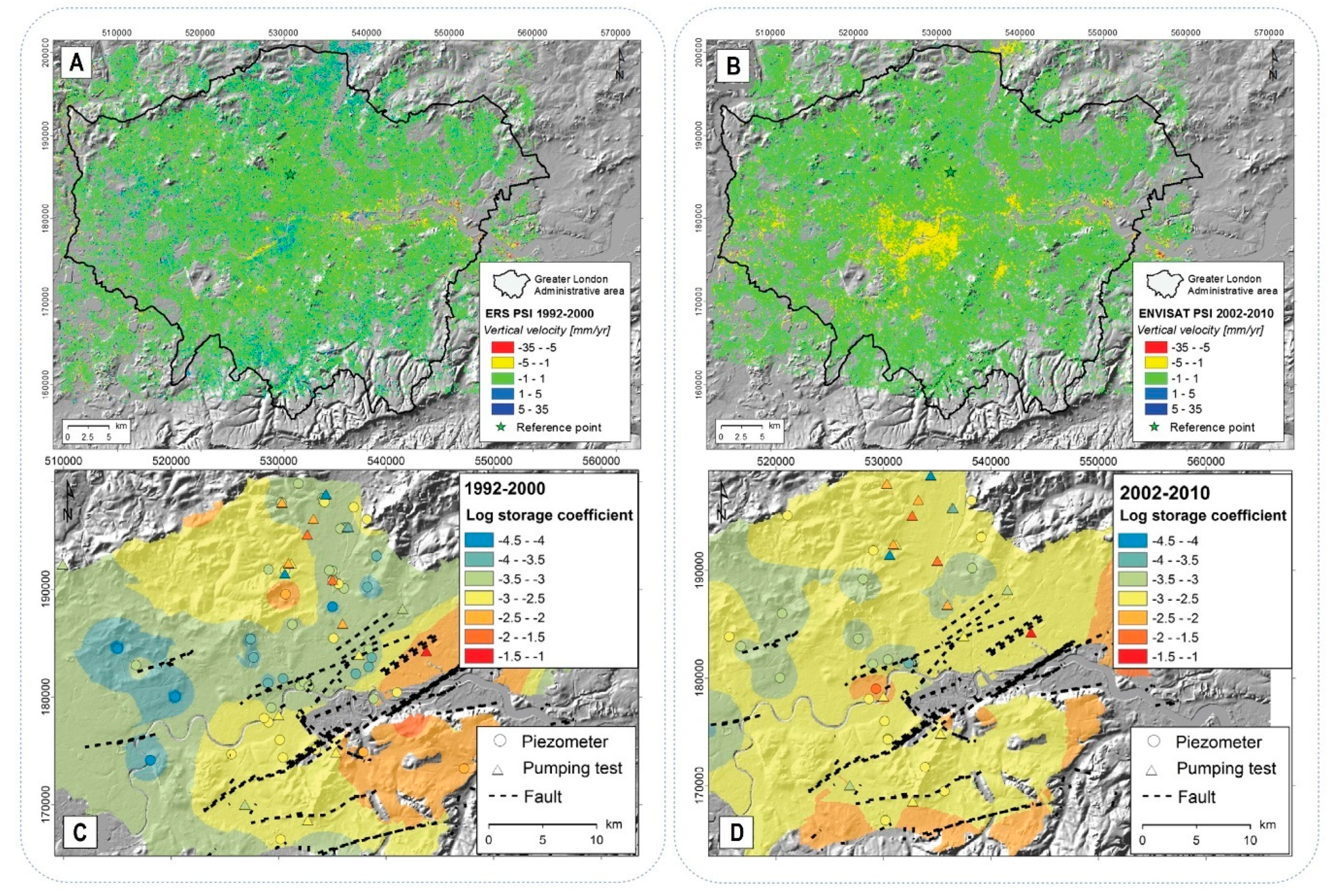
Over the past two decades, many studies have been conducted to integrate InSAR time-series analysis and groundwater head changes to estimate the storage coefficient [21,33,95,232,233,234,235]. A simple 1-D model proposed by Hofmann et al. [83] is mainly used to estimate the value of the parameter based on the inversion of Equation (9) (see Section 3.2). The model is also used to characterise the relationship between groundwater head and land surface motion time-series data to assess the contrast in ground motion across different geological units and under different aquifer conditions. The 1-D model assumes that the aquifer pore-water pressure balances instantaneously with the piezometric level changes in the aquifer and any time-lag between the piezometer level variations and the compaction of the geological layers is not accounted for.

Moreover, estimation of the aquifer storativity based on InSAR data paves the way for further investigations of the aquifer properties. The elastic skeletal specific storage of the confined aquifer can be derived from the inversion of Equation (4). Simultaneously, the elastic skeletal specific storage can be simply converted to values of aquifer matrix compressibility following Equation (4). InSAR combined with hydraulic data allows characterizing the aquifer-system properties at a basin scale. In cases where seasonal deformation is elastic and relatively constant over time, the storativity and elastic skeletal specific storage can be easily calculated, using averages of seasonal deformation and hydraulic head changes even if covering different periods. In locations where most of the seasonal effects are limited to the confined aquifer (little water being lost from the aquifer by outflow and evaporation), groundwater pumping rates can also be derived.

The success of using InSAR-derived deformation to predict hydraulic head changes depends on the amplitude of the deformation and of the seasonal hydraulic head changes. Therefore, InSAR data can primarily be used for the estimation of such changes for confined aquifers. The prediction accuracy also depends on the mode of deformation. The elastic range of aquifer deformation corresponds to storativity constant over time, whereas areas with high clay content characterised by a delayed deformation of low-permeability aquitards may require multiple calibration periods [171]. Nevertheless, in confined aquifers with large elastic seasonal hydraulic head changes, InSAR can be used to evaluate hydraulic head changes with high accuracy almost without well measurements [171].

The study carried out by Boni et al. [23] is one of the examples of integration between observed groundwater levels and satellite-derived displacement time-series for estimation of the spatio-temporal variations of the aquifer storage coefficient. PSInSAR land surface motion data have been used to estimate the storage coefficient in the London Basin and to understand the spatio-temporal variability of this parameter under different aquifer conditions. Such an analysis was undertaken by exploiting ground motion data for the years 1992–2000 and 2002–2010 (Figure 12A,B), obtained by processing two stacks of ERS-1/2 and ENVISAT radar imagery by using the Interferometric Point Target Analysis (IPTA) technique. The analysis allows the characterisation of the Chalk aquifer storage over an area of about 1360 km² (Figure 12C,D).

In addition, the increased sensitivity brought by latest developments in InSAR offers great potential for land surface motion detection induced by non-anthropogenic changes in groundwater storage, likely slower than for groundwater depletion in the vicinity of pumping centres [236,237]. InSAR would be able to provide a perspective on the relative importance of the anthropogenic and non-anthropogenic components of a change in groundwater storage. Non-anthropogenic storage change and induced land surface motion are expected to be close to or lower than the typical InSAR detection threshold of a few 3 to 5 mm/year. As a result, the most important parameter for such an application is the accuracy of InSAR measurements in natural settings.

5.2. InSAR Limitations in Groundwater-Induced Land Displacement Studies

The main challenge of InSAR application to groundwater-related land displacement studies is the loss of coherence in the natural system. This loss is usually proportional to the density of the vegetation and inversely proportional to the SAR wavelength. While patches of trees in urban areas are usually smoothed by down-sampling or are compensated by the interpolation of final results, lack of coherence is a problem where high vegetation is dominant throughout the land surface area. For example, short-wavelength SAR (X-band) would not allow the detection of land displacement in farmland and coherence could only be sufficient in urban areas. To overcome this problem, longer SAR wavelengths (C-band, L-band) can be used at the cost of higher displacement detection threshold and a lower vertical precision of the displacement estimation. Atmospheric effects also affect InSAR results in the range of cm/year. However, they can be almost entirely estimated and therefore reduced methodological improvements and, e.g., A-DInSAR processing techniques. In hydrogeology, displacement detected by InSAR is often assumed to be completely related to aquifer compaction. On a cm/year scale, aquifer spatial compaction patterns are usually well distinguished from sediment erosion, sediment deposition, landslides, volcanism, tectonic fault movements or mining. While the potential use of retrieving ground displacements on a mm/year scale is essential, their interpretation presents a concern when multiple causes of displacement may coexist.

It is expected that the SAR phase should be comparable between successive acquisitions. If the differential movement between two acquisitions of a SAR time-series is higher than the length of the SAR wave phase, and if this movement is not spatially progressive, the “jump” phase occurs and the inversion of the phase into displacement is compromised. Therefore, the temporal density of the InSAR image stack should be consistent with the expected rates of ground motion. Therefore, to make the optimal use of InSAR data, the time baseline of the SAR acquisition (and the SAR sensor) could be compared with the ground motion rate. These rates can often be expected approximately, taking into account previous hydrogeological knowledge of the area, other available ground displacement measurements or comparable cases are available in the previous SAR studies. Ideally, for example, to obtain a constant subsidence rate values of 5 cm/year based on the original PSI technique, the time-series of radar images should be consisted of at least seven, four and one images per year in the X-band, the C-band and the L-band, respectively [213]. If the subsidence is spatially progressive, more substantial subsidence rates can be extracted by the unwrapping of the spatial phase typically used in SBAS technique and implemented in some PSI algorithms. In such cases, other parameters should be taken into account. These include the noise level of the SAR data, the phase unwrapping technique and the temporal variability of the land surface displacement.

6. Concluding Remarks

In this review, we presented the general principles of models used to predict land surface displacements induced by aquifer drainage. We also aimed to summarize the implementation of InSAR data over the last few years to support the process of modelling the phenomenon and, therefore, discussed recent developments in modelling land surface displacements resulting from groundwater withdrawal.

The mechanisms underlying groundwater-induced land surface displacement are well understood and widely accepted, and the mathematical modelling of past events and expected future developments is relatively well developed. The mathematical models presented in this review are merely a general overview of the available solutions that can be found in research papers. Several key trends can be distinguished in the approaches presented, based on which new concepts and methods are being developed. The choice of the optimal method is usually determined by the availability of data required for model parametrization. Theoretical methods are a holistic approach to this issue. They take into account both the physical, hydrogeological and geomechanical properties of the aquifer system and groundwater. The use of these methods requires a comprehensive understanding of the aquifer properties. These models are therefore difficult to implement, especially in regions where there is a poor understanding of the physical, hydrogeological and geomechanical properties of the rock mass. The use of theoretical methods in advanced numerical models using modern computer technology, however, allows the simulation of the complex geologies and geometries of aquifers, arbitrarily arranged pumping wells, heterogeneity, anisotropy and non-linearity of the properties of porous media, which could only be done with an unacceptable degree of accuracy only a few years ago.

In the event of insufficient knowledge of the parameters of the aquifer system, semi-theoretical, empirical or influence function methods may be used to predict land subsidence. The implementation of these methods is relatively simple compared with theoretical approaches. Semi-theoretical models use generalized information describing the basic physical, hydrogeological and geomechanical constraints of the aquifer. The overall nature of the compaction process, however, is not taken into account in the calculations. Empirical methods use the information on the current state of land subsidence to predict the phenomenon in the short term. These methods do not take into account the physical, hydrogeological and geomechanical properties of the rock mass. Methods based on influence functions employ experiments and techniques that are commonly used by the mining industry in the case of land subsidence predictions due to the exploitation of mineral resources. The analysis and simulation of this type of subsidence using the influence function method involves the general assessment of factors that are often quite complex and difficult to interpret and classify clearly.

Notably, there has been a significant increase in interest in recent years in the use of AI techniques in modelling phenomena that require a significant degree of parametrization. The main advantage of using AI methods is their ability to discover complex relationships between individual data sets and to find and study hidden features in the data itself. This is not possible using traditional methods of prediction. However, a relatively small number of implementations of these methods report satisfactory modelling results, indicating the need for further research in this field.

The measurement and monitoring of anthropogenic land subsidence is currently at a very advanced stage, particularly with the use of satellite technology. Scientists can help decision-makers successfully predict, prevent or at least mitigate the phenomenon. Land subsidence detection takes advantage of a variety of options with respect to resolution, image footprint and precision from several SAR imaging spacecraft currently in operation. Radar images range in scale from semi-continental to building scale. Vertical precision usually ranges from millimetres when using short waves to centimetres when using long waves. Shorter waves allow for better vertical precision, while longer waves allow for better detection in less coherent areas. Although there have been no studies on remote detection of aquifer confinement by analysis of the spatial patterns of land subsidence, this is theoretically possible with minimal lithological data. Indeed, due to the significant difference in storativity, confined aquifers have a larger radius of influence and head drop than unconfined aquifers, which could be reflected in the amplitude and extent of the land subsidence. However, GRACE is sensitive to changes in mass over large spatial scales (more than 100,000 km²) and seems to be a promising method for detecting changes in storativity in confined aquifers [35,238]. Case studies in well-known hydrogeological settings, where in situ data are available, would make it possible to better understand the remaining challenges of such applications. There is, however, both hope and expectation for a valid option in the future for the remote assessment of aquifer confinement and groundwater flow dynamics.

Further research is needed to improve the assessment, analysis and forecasting of processes related to the compaction of susceptible aquifers and associated land subsidence to support water resource management and to identify measures for mitigating potential hazards. The main thematic areas of research suggested include the hydromechanical behaviour of aquitards, the role of horizontal deformation, and the regional simulation of combined groundwater flow and aquifer deformation. Given the substantial increase in the amount of measurement data derived from InSAR observations, further avenues of research in this field are also indicated. Particularly noteworthy is the role of AI in the processing of Big Data and the use of statistical tools for assessing the uncertainty of the model parameters and the results of modelling land surface displacements induced by aquifer drainage.

As groundwater demand increases globally, more reservoirs are experiencing land surface displacement, making it essential that to be able to accurately model the impacts of groundwater depletion and develop effective management strategies for the reduction or prevention of land subsidence. InSAR data is being acquired on a global scale, and the acquisition of such data is increasing to map groundwater systems. The integration of modelling approaches with InSAR data sets therefore provides a new way of obtaining accurate models of aquifer compaction driven by changes in groundwater systems.

References

- Gambolati, G.; Ricceri, G.; Bertoni, W.; Brighenti, G.; Vuillermin, E. Mathematical Simulation of the Subsidence of Ravenna. Water Resour. Res. 1991, 27, 2899–2918. [Google Scholar] [CrossRef]
- Ortega-Guerrero, A.; Rudolph, D.L.; Cherry, J.A. Analysis of Long-Term Land Subsidence near Mexico City: Field Investigations and Predictive Modeling. Water Resour. Res. 1999, 35, 3327–3341. [Google Scholar] [CrossRef]
- Ehlen, J.; Haneberg, W.C.; Larson, R.A.; Holzer, T.L.; Galloway, D.L. Impacts of Land Subsidence Caused by Withdrawal of Underground Fluids in the United States. In Humans as Geologic Agents; Geological Society of America: Boulder, CO, USA, 2007; Volume 16, pp. 87–99. [Google Scholar] [CrossRef] [Green Version]
- Teatini, P.; Ferronato, M.; Gambolati, G.; Gonella, M. Groundwater Pumping and Land Subsidence in the Emilia-Romagna Coastland, Italy: Modeling the Past Occurrence and the Future Trend. Water Resour. Res. 2006, 42. [Google Scholar] [CrossRef]
- Shi, X.Q.; Xue, Y.Q.; Ye, S.J.; Wu, J.C.; Zhang, Y.; Yu, J. Characterization of Land Subsidence Induced by Groundwater Withdrawals in Su-Xi-Chang Area, China. Environ. Geol. 2007, 52, 27–40. [Google Scholar] [CrossRef]
- Allis, R.; Bromley, C.; Currie, S. Update on Subsidence at the Wairakei-Tauhara Geothermal System, New Zealand. Geothermics 2009, 38, 169–180. [Google Scholar] [CrossRef]
- Mahmoudpour, M.; Khamehchiyan, M.; Nikudel, M.R.; Ghassemi, M.R. Characterization of Regional Land Subsidence Induced by Groundwater Withdrawals in Tehran, Iran. Geopersia 2013, 3, 49–62. [Google Scholar] [CrossRef]
- Erkens, G.; Bucx, T.; Dam, R.; De Lange, G.; Lambert, J. Sinking Coastal Cities. Proc. Int. Assoc. Hydrol. Sci. 2015. [Google Scholar] [CrossRef] [Green Version]
- Famiglietti, J.S.; Lo, M.; Ho, S.L.; Bethune, J.; Anderson, K.J.; Syed, T.H.; Swenson, S.C.; De Linage, C.R.; Rodell, M. Satellites Measure Recent Rates of Groundwater Depletion in California’s Central Valley. Geophys. Res. Lett. 2011, 38. [Google Scholar] [CrossRef] [Green Version]
- Whittaker, B.N.; Reddish, D.J. Subsidence: Occurrence, Prediction, and Control; Elsevier: Amsterdam, The Netherlands, 1989. [Google Scholar]
- Gambolati, G.; Teatini, P. Geomechanics of Subsurface Water Withdrawal and Injection. Water Resour. Res. 2015, 51, 3922–3955. [Google Scholar] [CrossRef]
- Wade, C.M.; Cobourn, K.M.; Amacher, G.S.; Hester, E.T. Policy Targeting to Reduce Economic Damages From Land Subsidence. Water Resour. Res. 2018, 54, 4401–4416. [Google Scholar] [CrossRef]
- Herrera, G.; Tomás, R.; Monells, D.; Centolanza, G.; Mallorquí, J.J.; Vicente, F.; Navarro, V.D.; Lopez-Sanchez, J.M.; Sanabria, M.; Cano, M. Analysis of Subsidence Using TerraSAR-X Data: Murcia Case Study. Eng. Geol. 2010, 116, 284–295. [Google Scholar] [CrossRef]
- Yang, Y.; Luo, Y.; Liu, M.; Wang, R.; Wang, H. Research of Features Related to Land Subsidence and Ground Fissure Disasters in the Beijing Plain. Proc. Int. Assoc. Hydrol. Sci. 2015. [Google Scholar] [CrossRef] [Green Version]
- Béjar-Pizarro, M.; Ezquerro, P.; Herrera, G.; Tomás, R.; Guardiola-Albert, C.; Ruiz Hernández, J.M.; Fernández Merodo, J.A.; Marchamalo, M.; Martínez, R. Mapping Groundwater Level and Aquifer Storage Variations from InSAR Measurements in the Madrid Aquifer, Central Spain. J. Hydrol. 2017, 547, 678–689. [Google Scholar] [CrossRef] [Green Version]
- Pratt, W.E.; Johnson, D.W. Local Subsidence of the Goose Creek Oil Field. J. Geol. 1926, 34, 577–590. [Google Scholar] [CrossRef]
- Shah, T. Groundwater and Human Development: Challenges and Opportunities in Livelihoods and Environment. Water Sci. Technol. 2005, 51, 27–37. [Google Scholar] [CrossRef]
- Galloway, D.L.; Burbey, T.J. Review: Regional Land Subsidence Accompanying Groundwater Extraction. Hydrogeol. J. 2011, 19, 1459–1486. [Google Scholar] [CrossRef]
- Amitrano, D.; Di Martino, G.; Iodice, A.; Mitidieri, F.; Papa, M.N.; Riccio, D.; Ruello, G. Sentinel-1 for Monitoring Reservoirs: A Performance Analysis. Remote Sens. 2014, 6, 10676–10693. [Google Scholar] [CrossRef] [Green Version]
- Bozzano, F.; Esposito, C.; Franchi, S.; Mazzanti, P.; Perissin, D.; Rocca, A.; Romano, E. Understanding the Subsidence Process of a Quaternary Plain by Combining Geological and Hydrogeological Modelling with Satellite InSAR Data: The Acque Albule Plain Case Study. Remote Sens. Environ. 2015, 168, 219–238. [Google Scholar] [CrossRef]
- Ezquerro, P.; Herrera, G.; Marchamalo, M.; Tomás, R.; Béjar-Pizarro, M.; Martínez, R. A Quasi-Elastic Aquifer Deformational Behavior: Madrid Aquifer Case Study. J. Hydrol. 2014, 519, 1192–1204. [Google Scholar] [CrossRef] [Green Version]
- Ezquerro, P.; Guardiola-Albert, C.; Herrera, G.; Fernández-Merodo, J.A.; Béjar-Pizarro, M.; Bonì, R. Groundwater and Subsidence Modeling Combining Geological and Multi-Satellite SAR Data over the Alto Guadalentín Aquifer (SE Spain). Geofluids 2017. [Google Scholar] [CrossRef]
- Bonì, R.; Cigna, F.; Bricker, S.; Meisina, C.; McCormack, H. Characterisation of Hydraulic Head Changes and Aquifer Properties in the London Basin Using Persistent Scatterer Interferometry Ground Motion Data. J. Hydrol. 2016, 540, 835–849. [Google Scholar] [CrossRef] [Green Version]
- Bonì, R.; Meisina, C.; Cigna, F.; Herrera, G.; Notti, D.; Bricker, S.; McCormack, H.; Tomás, R.; Béjar-Pizarro, M.; Mulas, J.; et al. Exploitation of Satellite A-DInSAR Time Series for Detection, Characterization and Modelling of Land Subsidence. Geosciences 2017, 7, 25. [Google Scholar] [CrossRef] [Green Version]
- Crosetto, M.; Monserrat, O.; Cuevas-González, M.; Devanthéry, N.; Crippa, B. Persistent Scatterer Interferometry: A Review. ISPRS J. Photogramm. Remote Sens. 2016, 115, 78–89. [Google Scholar] [CrossRef] [Green Version]
- Ferretti, A.; Fumagalli, A.; Novali, F.; Prati, C.; Rocca, F.; Rucci, A. A New Algorithm for Processing Interferometric Data-Stacks: SqueeSAR. IEEE Trans. Geosci. Remote Sens. 2011, 49, 3460–3470. [Google Scholar] [CrossRef]
- Hooper, A.J. A Multi-Temporal InSAR Method Incorporating Both Persistent Scatterer and Small Baseline Approaches. Geophys. Res. Lett. 2008, 35. [Google Scholar] [CrossRef] [Green Version]
- Cigna, F.; Tapete, D.; Garduño-Monroy, V.H.; Muñiz-Jauregui, J.A.; García-Hernández, O.H.; Jiménez-Haro, A. Wide-Area InSAR Survey of Surface Deformation in Urban Areas and Geothermal Fields in the Eastern Trans-Mexican Volcanic Belt, Mexico. Remote Sens. 2019, 11, 2341. [Google Scholar] [CrossRef] [Green Version]
- Farolfi, G.; Del Soldato, M.; Bianchini, S.; Casagli, N. A Procedure to Use GNSS Data to Calibrate Satellite PSI Data for the Study of Subsidence:An Example from the North-Western Adriatic Coast (Italy). Eur. J. Remote. Sens. 2019, 1–10. [Google Scholar] [CrossRef] [Green Version]
- Morishita, Y.; Lazecky, M.; Wright, T.J.; Weiss, J.R.; Elliott, J.R.; Hooper, A. LiCSBAS: An Open-Source Insar Time Series Analysis Package Integrated with the LiCSAR Automated Sentinel-1 InSAR Processor. Remote Sens. 2020, 12, 424. [Google Scholar] [CrossRef] [Green Version]
- European Space Agency. Sentinel-1—Missions—Sentinel. Available online: https://sentinel.esa.int/web/sentinel/missions/sentinel-1 (accessed on 21 March 2020).
- Poland, J.F. Guidebook to Studies of Land Subsidence Due to Ground-Water Withdrawal; UNESCO: Paris, France, 1984. [Google Scholar]
- Tomas, R.; Herrera, G.; Cooksley, G.; Mulas, J. Persistent Scatterer Interferometry Subsidence Data Exploitation Using Spatial Tools: The Vega Media of the Segura River Basin Case Study. J. Hydrol. 2011, 400, 411–428. [Google Scholar] [CrossRef]
- Taylor, R.G.; Scanlon, B.; Döll, P.; Rodell, M.; Van Beek, R.; Wada, Y.; Longuevergne, L.; Leblanc, M.; Famiglietti, J.S.; Edmunds, M.; et al. Ground water and climate change. Nat. Clim. Chang. 2012, 3, 322–329. [Google Scholar] [CrossRef] [Green Version]
- Wada, Y.; Van Beek, L.P.H.; Van Kempen, C.M.; Reckman, J.W.T.M.; Vasak, S.; Bierkens, M.F.P. Global Depletion of Groundwater Resources. Geophys. Res. Lett. 2010, 37. [Google Scholar] [CrossRef] [Green Version]
- Wada, Y.; Bierkens, M.F.P. Sustainability of Global Water Use: Past Reconstruction and Future Projections. Environ. Res. Lett. 2014, 9. [Google Scholar] [CrossRef]
- Allison, M.; Yuill, B.; Törnqvist, T.; Amelung, F.; Dixon, T.; Erkens, G.; Stuurman, R.; Jones, C.; Milne, G.; Steckler, M.; et al. Global Risks and Research Priorities for Coastal Subsidence. Eos 2016, 97. [Google Scholar] [CrossRef]
- Hu, B.; Chen, X.; Zhang, X. Using Multisensor SAR Datasets to Monitor Land Subsidence in Los Angeles from 2003 to 2017. J. Sens. 2019. [Google Scholar] [CrossRef] [Green Version]
- Castellazzi, P.; Arroyo-Domínguez, N.; Martel, R.; Calderhead, A.I.; Normand, J.C.L.; Gárfias, J.; Rivera, A. Land Subsidence in Major Cities of Central Mexico: Interpreting InSAR-Derived Land Subsidence Mapping with Hydrogeological Data. Int. J. Appl. Earth Obs. Geoinf. 2016, 47, 102–111. [Google Scholar] [CrossRef]
- Jones, C.E.; An, K.; Blom, R.G.; Kent, J.D.; Ivins, E.R.; Bekaert, D.P. Anthropogenic and Geologic Influences on Subsidence in the Vicinity of New Orleans, Louisiana. J. Geophys. Res. Solid Earth 2016. [Google Scholar] [CrossRef]
- Thoang, T.T.; Giao, P.H. Subsurface Characterization and Prediction of Land Subsidence for HCM City, Vietnam. Eng. Geol. 2015, 199, 107–124. [Google Scholar] [CrossRef]
- Pirouzi, A.; Eslami, A. Ground Subsidence in Plains around Tehran: Site Survey, Records Compilation and Analysis. Int. J. Geo-Eng. 2017. [Google Scholar] [CrossRef] [Green Version]
- Aobpaet, A.; Cuenca, M.C.; Hooper, A.; Trisirisatayawong, I. InSAR Time-Series Analysis of Land Subsidence in Bangkok, Thailand. Int. J. Remote Sens. 2013, 34, 2969–2982. [Google Scholar] [CrossRef]
- Guo, L.; Gong, H.; Zhu, F.; Zhu, L.; Zhang, Z.; Zhou, C.; Gao, M.; Sun, Y. Analysis of the Spatiotemporal Variation in Land Subsidence on the Beijing Plain, China. Remote Sens. 2019, 11, 1170. [Google Scholar] [CrossRef] [Green Version]
- Jafari, F.; Javadi, S.; Golmohammadi, G.; Karimi, N.; Mohammadi, K. Numerical Simulation of Groundwater Flow and Aquifer-System Compaction Using Simulation and InSAR Technique: Saveh Basin, Iran. Environ. Earth Sci. 2016, 75. [Google Scholar] [CrossRef]
- Rahmawati, N.; Vuillaume, J.F.; Purnama, I.L.S. Salt Intrusion in Coastal and Lowland Areas of Semarang City. J. Hydrol. 2013, 494, 146–159. [Google Scholar] [CrossRef]
- Faunt, C.C.; Sneed, M.; Traum, J.; Brandt, J.T. Water Availability and Land Subsidence in the Central Valley, California, USA. Hydrogeol. J. 2016, 24, 675–684. [Google Scholar] [CrossRef] [Green Version]
- Maps—UNESCO Land Subsidence International Initiative. Available online: https://www.landsubsidence-unesco.org/maps/ (accessed on 2 June 2020).
- Center for International Earth Science Information Network—CIESIN—Columbia University. Gridded Population of the World, Version 4 (GPWv4): Population Density, Revision 11; NASA Socioeconomic Data and Applications Center (SEDAC): Palisades, NY, USA, 2018. [CrossRef]
- Hole, J.K.; Bromley, C.J.; Stevens, N.F.; Wadge, G. Subsidence in the Geothermal Fields of the Taupo Volcanic Zone, New Zealand from 1996 to 2005 Measured by InSAR. J. Volcanol. Geotherm. Res. 2007, 166, 125–146. [Google Scholar] [CrossRef]
- Chaussard, E.; Wdowinski, S.; Cabral-Cano, E.; Amelung, F. Land Subsidence in Central Mexico Detected by ALOS InSAR Time-Series. Remote Sens. Environ. 2014, 140, 94–106. [Google Scholar] [CrossRef]
- Hu, R.L.; Yue, Z.Q.; Wang, L.C.; Wang, S.J. Review on Current Status and Challenging Issues of Land Subsidence in China. Eng. Geol. 2004, 76, 65–77. [Google Scholar] [CrossRef]
- Zhu, L.; Gong, H.; Li, X.; Wang, R.; Chen, B.; Dai, Z.; Teatini, P. Land Subsidence Due to Groundwater Withdrawal in the Northern Beijing Plain, China. Eng. Geol. 2015, 193, 243–255. [Google Scholar] [CrossRef]
- Qin, H.; Andrews, C.B.; Tian, F.; Cao, G.; Luo, Y.; Liu, J.; Zheng, C. Groundwater-pumping optimization for land-subsidence control in Beijing plain, China. Hydrogeol. J. 2018, 26, 1061–1081. [Google Scholar] [CrossRef]
- Why Indonesia’s Government Is Moving Capital from Jakarta to a “Strategic Location” in Borneo. Available online: https://www.telegraph.co.uk/news/2019/08/26/indonesias-government-reveals-location-new-capital-jakarta-sinks/ (accessed on 2 June 2020).
- Sinking Basilica in Mexico City. Available online: https://www.usgs.gov/media/images/sinking-basilica-mexico-city (accessed on 2 June 2020).
- Earth Fissure in Residential Area of Chandler Heights, Arizona, AZGS. Available online: https://azgs.arizona.edu/photo/earth-fissure-residential-area-chandler-heights-arizona (accessed on 2 June 2020).
- International Hydrological Programme. Available online: http://www.unesco.org/new/en/natural-sciences/environment/water/ihp/about-ihp/ (accessed on 9 April 2020).
- Tenth International Symposium on Land Subsidence. Available online: https://www.tisols2020.org/tisols2020 (accessed on 9 April 2020).
- Tison, L.J. Land Subsidence: Proceedings of the Tokyo Symposium, September, 1969, Tokyo, Japan; IAHS-UNESCO, The University of Virginia: Charlottesville, VA, USA, 1970. [Google Scholar]
- Johnson, A.I. Land Subsidence Symposium. Eos 1977, 58, 302. [Google Scholar] [CrossRef]
- Johnson, A.I.; Carbognin, L.; Ubertini, L. Land Subsidence. In Proceedings of the 3rd International Symposium, Venice, Italy, 19–25 March 1984; IAHS Publication: Wallingford, UK, 1986. [Google Scholar]
- Johnson, A.I. Proceedings of the Fourth International Symposium on Land Subsidence, Houston, TX, USA; IAHS Press, Institute of Hydrology: Wallingford, Oxfordshire, UK, 1991. [Google Scholar]
- Barends, F.B.J.; Brouwer, F.J.J.; Schröder, F.H. Land Subsidence: Natural Causes, Measuring Techniques, the Groningen Gasfields. In Proceedings of the Fifth International Symposium on Land Subsidence, The Hague, The Netherlands, 16–20 October 1995; CRC Press: Boca Raton, FL, USA, 1995. [Google Scholar]
- Carbognin, L.; Gambolati, G.; Johnson, A. Land Subsidence: Proceedings of the Sixth International Symposium on Land Subsidence, Ravenna, Italia, 24–29 September 2000; C.N.R: Roma, Italia, 2000. [Google Scholar]
- Zhang, A.; Gong, S.; Carbognin, L.; Johnson, A.I.; Arnold, I. Proceedings of the Seventh International Symposium on Land Subsidence, Held in Shanghai, China; Shanghai Institute of Geological Survey: Shanghai, China, 2005. [Google Scholar]
- Carreón-Freyre, D.; Cerca, M.; Galloway, D.L.; Silva-Corona, J.J.; International Association of Hydrological Sciences. Land Subsidence, Associated Hazards and the Role of Natural Resources Development; International Association of Hydrological Sciences: Wallingford, UK, 2010; Volume 339. [Google Scholar]
- Daito, K.; Galloway, D.L. Preface: Prevention and Mitigation of Natural and Anthoropogenic Hazards Due to Land Subsidence. Proc. Int. Assoc. Hydrol. Sci. 2015, 372, 555–557. [Google Scholar] [CrossRef]
- Konikow, L.F. Long-Term Groundwater Depletion in the United States. Ground Water 2014, 53, 2–9. [Google Scholar] [CrossRef] [PubMed]
- Gleeson, T.; Alley, W.M.; Allen, D.M.; Sophocleous, M.A.; Zhou, Y.; Taniguchi, M.; Vandersteen, J. Towards Sustainable Groundwater Use: Setting Long-Term Goals, Backcasting, and Managing Adaptively. Ground Water 2012, 50, 19–26. [Google Scholar] [CrossRef] [PubMed]
- Landes, A.A.L.; Aquilina, L.; De Ridder, J.; Longuevergne, L.; Page, C.; Goderniaux, P. Investigating the respective impacts of groundwater exploitation and climate change on wetland extension over 150 years. J. Hydrol. 2014, 509, 367–378. [Google Scholar] [CrossRef] [Green Version]
- De Marsily, G.; DeLay, F.; Gonçalves, J.; Renard, P.; Teles, V.; Violette, S.; Renard, P. Dealing with spatial heterogeneity. Hydrogeol. J. 2005, 13, 161–183. [Google Scholar] [CrossRef]
- Freeze, R.A.; Cherry, A.J. Groundwater; Prentice-Hall: Englewood Cliffs, NJ, USA, 1979. [Google Scholar]
- Fetter, C.W. Applied Hydrogeology, 4th ed.; Waveland Press: Long Grove, IL, USA, 2018. [Google Scholar]
- Balkhair, K.S. Aquifer Parameters Determination for Large Diameter Wells Using Neural Network Approach. J. Hydrol. 2002, 265, 118–128. [Google Scholar] [CrossRef]
- Schad, H.; Teutsch, G. Effects of the Investigation Scale on Pumping Test Results in Heterogeneous Porous Aquifers. J. Hydrol. 1994, 159, 61–77. [Google Scholar] [CrossRef]
- Kaczmaryk, A.; DeLay, F. Interference pumping tests in a fractured limestone (Poitiers—France): Inversion of data by means of dual-medium approaches. J. Hydrol. 2007, 337, 133–146. [Google Scholar] [CrossRef]
- Jacob, C.E. On the Flow of Water in an Elastic Artesian Aquifer. Trans. Am. Geophys. Union 1940, 21, 574. [Google Scholar] [CrossRef]
- Biot, M.A. General Theory of Three-Dimensional Consolidation. J. Appl. Phys. 1941, 12, 155. [Google Scholar] [CrossRef]
- Terzaghi, K. Principles of Soil Mechanics: IV-Settlement and Consolidation of Clay. Eng. News-Rec. 1925, 95, 742–746. [Google Scholar]
- Terzaghi, K. Theoretical Soil Mechanics; John Wiley & Sons: Hoboken, NJ, USA, 1943. [Google Scholar] [CrossRef]
- Cooper, H.H. The Equation of Groundwater Flow in Fixed and Deforming Coordinates. J. Geophys. Res. 1966, 71, 4785–4790. [Google Scholar] [CrossRef]
- Hoffmann, J.; Zebker, H.A.; Galloway, D.L.; Amelung, F. Seasonal Subsidence and Rebound in Las Vegas Valley, Nevada, Observed by Synthetic Aperture Radar Interferometry. Water Resour. Res. 2001, 37, 1551–1566. [Google Scholar] [CrossRef]
- Zhang, Y.; Xue, Y.; Wu, J.-C.; Ye, S.; Wei, Z.-X.; Li, Q.-F.; Yu, J. Characteristics of aquifer system deformation in the Southern Yangtse Delta, China. Eng. Geol. 2007, 90, 160–173. [Google Scholar] [CrossRef]
- Theis, C.V. The Relation between the Lowering of the Piezometric Surface and the Rate and Duration of Discharge of a Well Using Ground-water Storage. Trans. Am. Geophys. Union 1935, 16, 519. [Google Scholar] [CrossRef]
- Cooper, H.H.; Jacob, C.E. A Generalized Graphical Method for Evaluating Formation Constants and Summarizing Well-field History. Eos Trans. Am. Geophys. Union 1946, 27, 526. [Google Scholar] [CrossRef]
- Pool, D.R.; Eychaner, J.H. Measurements of Aquifer-Storage Change and Specific Yield Using Gravity Surveys. Ground Water 1995, 33, 425–432. [Google Scholar] [CrossRef]
- Gehman, C.L.; Harry, D.L.; Sanford, W.E.; Stednick, J.D.; Beckman, N.A. Estimating Specific Yield and Storage Change in an Unconfined Aquifer Using Temporal Gravity Surveys. Water Resour. Res. 2009, 45. [Google Scholar] [CrossRef]
- Poland, J.F.; Davis, G.H. Land Subsidence Due to Withdrawal of Fluids. Landslides 1969, 2, 187–270. [Google Scholar] [CrossRef]
- Chilingarian, G.V.; Donaldson, E.C.; Yen, T.F. Subsidence Due to Fluid Withdrawal. Int. J. Rock Mech. Min. Sci. Géoméch. Abstr. 1996, 33. [Google Scholar] [CrossRef]
- Wilson, A.M.; Gorelick, S. The Effects of Pulsed Pumping on Land Subsidence in the Santa Clara Valley, California. J. Hydrol. 1996, 174, 375–396. [Google Scholar] [CrossRef]
- Amelung, F.; Galloway, D.L.; Bell, J.W.; Zebker, H.A.; Laczniak, R.J. Sensing the Ups and Downs of Las Vegas: InSAR Reveals Structural Control of Land Subsidence and Aquifer-System Deformation. Geology 1999, 27, 483–486. [Google Scholar] [CrossRef]
- Lu, Z.; Danskin, W.R. InSAR Analysis of Natural Recharge to Define Structure of a Ground-Water Basin, San Bernardino, California. Geophys. Res. Lett. 2001, 28, 2661–2664. [Google Scholar] [CrossRef] [Green Version]
- Schmidt, D.A.; Bürgmann, R. Time-Dependent Land Uplift and Subsidence in the Santa Clara Valley, California, from a Large Interferometric Synthetic Aperture Radar Data Set. J. Geophys. Res. Solid Earth 2003, 108. [Google Scholar] [CrossRef] [Green Version]
- Chaussard, E.; Bürgmann, R.; Shirzaei, M.; Fielding, E.J.; Baker, B. Predictability of Hydraulic Head Changes and Characterization of Aquifer-System and Fault Properties from InSAR-Derived Ground Deformation. J. Geophys. Res. Solid Earth 2014, 119, 6572–6590. [Google Scholar] [CrossRef]
- Hammond, W.C.; Burgette, R.J.; Johnson, K.M.; Blewitt, G. Uplift of the Western Transverse Ranges and Ventura Area of Southern California: A Four-Technique Geodetic Study Combining GPS, InSAR, Leveling, and Tide Gauges. J. Geophys. Res. Solid Earth 2018, 123, 836–858. [Google Scholar] [CrossRef]
- Hu, X.; Lu, Z.; Wang, T. Characterization of Hydrogeological Properties in Salt Lake Valley, Utah, Using InSAR. J. Geophys. Res. Earth Surf. 2018, 123, 1257–1271. [Google Scholar] [CrossRef]
- Chaussard, E.; Milillo, P.; Bürgmann, R.; Perissin, D.; Fielding, E.J.; Baker, B. Remote Sensing of Ground Deformation for Monitoring Groundwater Management Practices: Application to the Santa Clara Valley During the 2012–2015 California Drought. J. Geophys. Res. Solid Earth 2017, 122, 8566–8582. [Google Scholar] [CrossRef]
- Riley, F.S. Analysis of borehole extensometer data from central California, in Land Subsidence, vol. 2, edited by L. K. Tison. Int. Assoc. Sci. Hydrol. 1969, 89, 423–431. [Google Scholar]
- Borchers, J.W.; Association of Engineering Geologists. Sacramento Section.; Association of Engineering Geologists. Subsidence Committee. Land Subsidence Case Studies and Current Research: Proceedings of the Dr. Joseph F. Poland Symposium on Land Subsidence; California Water Foundation: Sacramento, CA, USA, 1998. [Google Scholar]
- Helm, D.C. One-Dimensional Simulation of Aquifer System Compaction. Water Resour. Res. 1975, 11, 465–478. [Google Scholar] [CrossRef]
- Helm, D.C. One-dimensional Simulation of Aquifer System Compaction near Pixley, California: 2. Stress-Dependent Parameters. Water Resour. Res. 1976, 12, 375–391. [Google Scholar] [CrossRef]
- Witherspoon, P.A.; Freeze, R.A. The Role of Aquitards in Multiple-Aquifer Systems. Trans. Am. Geophys. Union 1972, 53, 743. [Google Scholar] [CrossRef]
- Gambolati, G.; Freeze, R.A. Mathematical Simulation of the Subsidence of Venice: 1. Theory. Water Resour. Res. 1973, 9, 721–733. [Google Scholar] [CrossRef]
- Narasimhan, T.N.; Witherspoon, P.A. Numerical Model for Land Subsidence in Shallow Groundwater Systems. In Proceedings of the Second International Symposium on Land Subsidence, Anaheim, CA, USA, 13–17 December 1976. [Google Scholar]
- Neuman, S.P.; Preller, C.; Narasimhan, T.N. Adaptive Explicit-implicit Quasi Three-dimensional Finite Element Model of Flow and Subsidence in Multiaquifer Systems. Water Resour. Res. 1982, 18, 1551–1561. [Google Scholar] [CrossRef]
- Helm, D.C. Field-Based Computational Techniques for Predicting Subsidence Due to Fluid Withdrawal. GSA Rev. Eng. Geol. 1984. [Google Scholar] [CrossRef]
- Helm, D.C. COMPAC: A Field-Tested Model to Simulate and Predict Subsidence Due to Fluid Withdrawal. Aust. Geomech. 1986. [Google Scholar] [CrossRef]
- Pope, J.P.; Burbey, T.J. Multiple-Aquifer Characterization from Single Borehole Extensometer Records. Ground Water 2004, 42, 45–58. [Google Scholar] [CrossRef]
- Liu, Y.; Helm, D.C. Inverse Procedure for Calibrating Parameters That Control Land Subsidence Caused by Subsurface Fluid Withdrawal: 1. Methods. Water Resour. Res. 2008, 44. [Google Scholar] [CrossRef]
- Liu, Y.; Helm, D.C. Inverse Procedure for Calibrating Parameters That Control Land Subsidence Caused by Subsurface Fluid Withdrawal: 2. Field Application. Water Resour. Res. 2008, 44. [Google Scholar] [CrossRef]
- Hung, W.C.; Hwang, C.; Liou, J.C.; Lin, Y.S.; Yang, H.L. Modeling Aquifer-System Compaction and Predicting Land Subsidence in Central Taiwan. Eng. Geol. 2012, 147, 78–90. [Google Scholar] [CrossRef]
- Prudic, D.E. Documentation of a Computer Program to Simulate Stream-Aquifer Relations Using a Modular, Finite-Difference Ground-Water Flow Model. U.S. Geol. Surv. 1989. [Google Scholar] [CrossRef]
- McDonald, M.G.; Harbaugh, A.W. A Modular Three-Dimensional Finite-Difference Groundwater Flow Model. U.S. Geol. Surv. 1984. [Google Scholar] [CrossRef]
- Larson, K.J.; Basagaoglu, H.; Mariño, M. Numerical Simulation of Land Subsidence in the Los Banos-Kettleman City Area, California; Contrib.—Univ. California, Water Resource Center: Irvine, CA, USA, 2001. [Google Scholar]
- Hanson, R.T.; Anderson, S.R.; Pool, D.R. Simulation of Ground-Water Flow and Potential Land Subsidence, Avra Valley, Arizona. U.S. Geol. Surv. 1990. [Google Scholar] [CrossRef]
- Hanson, R.T.; Benedict, J.F. Simulation of Ground-Water Flow and Potential for Land Subsidence, Upper Santa Cruz Basin, Arizona. U.S. Geol. Surv. 1994. [Google Scholar] [CrossRef]
- Galloway, D.L.; Hudnut, K.W.; Ingebritsen, S.E.; Phillips, S.P.; Peltzer, G.; Rogez, F.; Rosen, P.A. Detection of Aquifer System Compaction and Land Subsidence Using Interferometric Synthetic Aperture Radar, Antelope Valley, Mojave Desert, California. Water Resour. Res. 1998, 34, 2573–2585. [Google Scholar] [CrossRef]
- Nishikawa, T.; Rewis, D.L.; Martin, P. Numerical Simulation of Ground-Water Flow and Land Subsidence at Edwards Air Force Base, Antelope Valley, California. U.S. Geol. Surv. 2001. [Google Scholar] [CrossRef]
- Kasmarek, M.C.; Strom, E.W. Hydrogeology and Simulation of Ground-Water Flow and Land-Surface Subsidence in the Chicot and Evangeline Aquifers, Houston Area, Texas. U.S. Geol. Surv. 2002. [Google Scholar] [CrossRef]
- Don, N.C.; Hang, N.T.M.; Araki, H.; Yamanishi, H.; Koga, K. Groundwater Resources Management under Environmental Constraints in Shiroishi of Saga Plain, Japan. Environ. Geol. 2006, 49, 601–609. [Google Scholar] [CrossRef]
- Leake, S.A. Interbed Storage Changes and Compaction in Models of Regional Groundwater Flow. Water Resour. Res. 1990, 26, 1939–1950. [Google Scholar] [CrossRef]
- Leake, S.A. Simulation of Vertical Compaction in Models of Regional Ground-Water Flow; International Association of Hydrological Sciences: Wallingford, UK, 1991; pp. 565–574. [Google Scholar] [CrossRef]
- Hoffmann, J.; Leake, S.A.; Galloway, D.L.; Wilson, A. MODFLOW-2000 Ground-Water Model—User Guide to the Subsidence and Aquifer-System Compaction (SUB) Package. U.S. Geol. Surv. 2003. [Google Scholar] [CrossRef] [Green Version]
- Harbaugh, B.A.W.; Banta, E.R.; Hill, M.C.; Mcdonald, M.G. MODFLOW-2000, The U.S. Geological Survey Modular Graound-Water Model—User Guide to Modularization Concepts and the Ground-Water Flow Process. U.S. Geol. Surv. 2000. [Google Scholar] [CrossRef] [Green Version]
- Harbaugh Arlen, W. MODFLOW-2005, The U.S. Geological Survey Modular Ground-Water Model—The Ground-Water Flow Process. U.S. Geol. Surv. 2005. [Google Scholar] [CrossRef] [Green Version]
- Faunt, C.C. Groundwater Availability of the Central Valley Aquifer, California. U.S. Geol. Surv. 2010. [Google Scholar] [CrossRef]
- Deng, X.; Li, F.; Zhao, Y.; Li, S. Regulation of Deep Groundwater Based on MODFLOW in the Water Intake Area of the South-to-North Water Transfer Project in Tianjin, China. J. Hydroinformatics 2018, 20, 989–1007. [Google Scholar] [CrossRef]
- Leake, S.A.; Galloway, D.L. MODFLOW Ground-Water Model—User Guide to the Subsidence and Aquifer-System Compaction Package (SUB-WT) for Water-Table Aquifers. U.S. Geol. Surv. 2007. [Google Scholar] [CrossRef]
- Leake, S.A.; Galloway, D.L. Use of the SUB-WT Package for MODFLOW to Simulate Aquifer-System Compaction in Antelope Valley, California, USA; International Association of Hydrological Sciences: Wallingford, UK, 2010. [Google Scholar]
- Al-Sittawy, M.; Gad, S.; Fouad, R.; Nofal, E. Assessment of Soil Subsidence Due to Long-Term Dewatering, Esna City, Egypt. Water Sci. 2019, 33, 40–53. [Google Scholar] [CrossRef] [Green Version]
- Kooi, H.; Yuherdha, A.T. Updated Subsidence Scenarios Jakarta MODFLOW SUB-CR Calculations for Sunter, Daan Mogot and Marunda; Deltares: Delft, The Netherlands, 2018. [Google Scholar]
- Vassena, C.; Giudici, M.; Ponzini, G. Modelling Land Subsidence Induced by Exploitation of a Multi-Layered Aquifer in Milan (Italy). Acta Universitatis Carolinae Geol. 2002, 46, 641–644. [Google Scholar]
- Verruijt, A. Elastic Storage of Aquifers. In Flow through Porous Media; De Wiest, R.J.M., Ed.; Academic Press: New York, NY, USA, 1969; pp. 331–376. [Google Scholar]
- Kumpel, H.J. Theory of Linear Poroelasticity with Applications to Geomechanics and Hydrogeology. Geophys. J. Int. 2002, 150, 828–829. [Google Scholar] [CrossRef] [Green Version]
- Ingebritsen, S.E.; Sanford, W.E. Groundwater in Geologic Processes; Cambridge University Press: Cambridge, UK, 1998; p. 536. [Google Scholar] [CrossRef]
- Hsieh, P.A. Deformation-Induced Changes in Hydraulic Head During Ground-Water Withdrawal. Ground Water 1996, 34, 1082–1089. [Google Scholar] [CrossRef]
- Burbey, T.J.; Helm, D.C. Modeling Three-Dimensional Deformation in Response to Pumping of Unconsolidated Aquifers. Environ. Eng. Geosci. 1999, 199–212. [Google Scholar] [CrossRef]
- Burbey, T.J. Stress-Strain Analyses for Aquifer-System Characterization. Ground Water 2001, 39, 128–136. [Google Scholar] [CrossRef]
- Burbey, T.J. The Influence of Faults in Basin-Fill Deposits on Land Subsidence, Las Vegas Valley, Nevada, USA. Hydrogeol. J. 2002, 10, 525–538. [Google Scholar] [CrossRef]
- Helm, D.C. Horizontal Aquifer Movement in a Theis-Thiem Confined System. Water Resour. Res. 1994, 30, 953–964. [Google Scholar] [CrossRef]
- Li, J. Transient Radial Movement of a Confined Leaky Aquifer Due to Variable Well Flow Rates. J. Hydrol. 2007, 333, 542–553. [Google Scholar] [CrossRef]
- Kim, J.-M.; Parizek, R.R. A Mathematical Model for the Hydraulic Properties of Deforming Porous Media. Ground Water 1999, 37, 546–554. [Google Scholar] [CrossRef]
- Aichi, M.; Tokunaga, T. Poroelastic Modeling to Assess the Effect of Water Injection for Land Subsidence Mitigation. Proc. Int. Assoc. Hydrol. Sci. 2015. [Google Scholar] [CrossRef] [Green Version]
- Li, J.; Helm, D.C. Using an analytical solution to estimate the subsidence risk caused by ASR applications. Environ. Eng. Geosci. 2001, 7, 67–79. [Google Scholar] [CrossRef]
- Li, J. A nonlinear elastic solution for 1-D subsidence due to aquifer storage and recovery applications. Hydrogeol. J. 2003, 11, 646–658. [Google Scholar] [CrossRef]
- Jackson, J.D.; Helm, D.C.; Brumley, J.C. The Role of Poroviscosity in Evaluating Land Subsidence Due to Groundwater Extraction from Sedimentary Basin Sequences. Geofis. Int. 2004, 43, 689–695. [Google Scholar]
- Taylor, D.W. Fundamentals of Soil Mechanics. Soil Sci. 1948, 66, 161. [Google Scholar] [CrossRef]
- Jeng, D.I. A Three-Dimensional Model of Poroviscous Aquifer Deformation. Ph.D. Thesis, Virginia Polytechnic Institute and State University, Blacksburg, VA, USA, 2005. [Google Scholar]
- Jiang, L.; Helm, D. A General Formulation for Saturated Aquifer Deformation under Dynamic and Viscous Conditions. In Land Subsidence. Proceedings to the International Symposium, The Hague, 1995; International Association of Hydrological Sciences: Wallingford, UK, 1995; Volume 234, pp. 323–332. [Google Scholar] [CrossRef]
- Li, J.; Helm, D.C. Numerical Formulation of Dynamic Behavior within Saturated Soil Characterized by Elasto-Viscous Behavior with an Application to Las Vegas Valley. In Computer Method and Advances in Geomechanics, Proceedings of the 9th International Conference of the International Association for Computer Method and Advances in Geomechanics, Wuhan, China 2–7 November 1997; Yuan, J.X., Ed.; CRC Press: Boca Raton, FL, USA, 1997; pp. 911–916. [Google Scholar]
- Schwartz, F.W.; Zhang, H. Fundamentals of Ground Water; John Wiley & Sons: Hoboken, NJ, USA, 2003. [Google Scholar]
- Yamaguchi, R. Change of Water Level of a Deep Weel in the University of Tokyo. Tokyo Univ. Earthq. Res. Inst. Bull. 1969, 47, 1093–1111. [Google Scholar]
- Shibasaki, T.; Shindo, T. The Hydrologic Balance in the Land Subsidence Phenomena. In IASH/UNESCO Tokyo Symposium on Land Subsidence; Tison, L.J., Ed.; International Association of Hydrological Sciences: Wallingford, UK, 1969; pp. 201–215. [Google Scholar]
- Hwang, J.M.; Wu, C.M. Land Subsidence Problems in Taipei Basin. In Proceedings of the Tokyo Symposium on Land Subsidence; International Association of Scientific Hydrology and UNESCO: Tokyo, Japan, 1969; pp. 21–34. [Google Scholar]
- Wolkersdorfer, C.; Thiem, G. Ground Water Withdrawal and Land Subsidence in Northeastern Saxony (Germany). Mine Water Environ. 1999, 18, 81–92. [Google Scholar] [CrossRef]
- Kenselaar, F.; Quadvlieg, R. Trend-Signal Modelling of Land Subsidence. In The 10th FIG International Symposium on Deformation Measurements, California, USA; Metropolitan Water District: Los Angeles, CA, USA, 2001; pp. 336–345. [Google Scholar]
- Guzy, A.; Ahmed, A.W.; Malinowska, A. Spatio-Temporal Distribution of Land Subsidence and Water Drop Caused by Underground Exploitation of Mineral Resources. In International Multidisciplinary Scientific GeoConference Surveying Geology and Mining Ecology Management; SGEM World Science: Wien, Austria, 2018. [Google Scholar] [CrossRef]
- Malinowska, A.; Hejmanowski, R.; Dai, H.y. Ground Movements Modeling Applying Adjusted Influence Function. Int. J. Min. Sci. Technol. 2020, 30, 243–249. [Google Scholar] [CrossRef]
- Brown, K.; Trott, S. Groundwater Flow Models in Open Pit Mining: Can We Do Better? Mine Water Environ. 2014, 33, 187–190. [Google Scholar] [CrossRef]
- Fokker, P.A.; Orlić, B. Semi-Analytic Modelling of Subsidence. Math. Geol. 2006, 38, 565–589. [Google Scholar] [CrossRef]
- Ren, G.; Buckeridge, J.; Li, J. Estimating Land Subsidence Induced by Groundwater Extraction in Unconfined Aquifers Using an Influence Function Method. J. Water Resour. Plan. Manag. 2015, 141. [Google Scholar] [CrossRef]
- Sroka, A.; Hejmanowski, R. Subsidence Prediction Caused by the Oil and Gas Development. In Proceedings of the 3rd/12th FIG Symposium, Baden, Germany, 22–24 May 2006. [Google Scholar]
- Knothe, S. Equation of the Subsidence Profile. Arch. Min. Metall. 1953, 1, 22–38. [Google Scholar]
- Knothe, S. Observations of Surface Movements under Influence of Mining and Their Theoretical Interpretation. In Proceedings of the European Congress on Ground Movement, Leeds, UK, 9–12 April 1957; pp. 210–218. [Google Scholar]
- Diaz-Fernandez, M.E.; Álvarez-Fernández, M.I.; Álvarez-Vigil, A.E. Computation of influence functions for automatic mining subsidence prediction. Comput. Geosci. 2010, 14, 83–103. [Google Scholar] [CrossRef]
- Burbey, T.J.; Zhang, M. Inverse Modeling Using PS-InSAR for Improved Calibration of Hydraulic Parameters and Prediction of Future Subsidence for Las Vegas Valley, USA. Proc. Int. Assoc. Hydrol. Sci. 2015. [Google Scholar] [CrossRef] [Green Version]
- Hejmanowski, R. Modeling of time dependent subsidence for coal and ore deposits. Int. J. Coal Sci. Technol. 2015, 2, 287–292. [Google Scholar] [CrossRef] [Green Version]
- Fokker, P.A.; Van Thienen-Visser, K. Inversion of double-difference measurements from optical leveling for the Groningen gas field. Int. J. Appl. Earth Obs. Geoinf. 2016, 49, 1–9. [Google Scholar] [CrossRef]
- Zoccarato, C.; Ferronato, M.; Teatini, P. Formation compaction vs land subsidence to constrain rock compressibility of hydrocarbon reservoirs. Géoméch. Energy Environ. 2018, 13, 14–24. [Google Scholar] [CrossRef]
- Hoffmann, J.; Galloway, D.L.; Zebker, H.A. Inverse modeling of interbed storage parameters using land subsidence observations, Antelope Valley, California. Water Resour. Res. 2003, 39. [Google Scholar] [CrossRef]
- McGovern, S.; Kollet, S.; Bürger, C.M.; Schwede, R.L.; Podlaha, O.G. Novel basin modelling concept for simulating deformation from mechanical compaction using level sets. Comput. Geosci. 2017, 148, 2–848. [Google Scholar] [CrossRef] [Green Version]
- Feng, X.-T.; Hudson, J.A. Specifying the information required for rock mechanics modelling and rock engineering design. Int. J. Rock Mech. Min. Sci. 2010, 47, 179–194. [Google Scholar] [CrossRef]
- Witkowski, W.T.; Hejmanowski, R. Software for Estimation of Stochastic Model Parameters for a Compacting Reservoir. Appl. Sci. 2020, 10, 3287. [Google Scholar] [CrossRef]
- Truplett, T.; Yurchak, D. Determination of Intensity Functions for Predicting Subsidence from Coal Mining, Potash Mining, and Groundwater Withdrawal Using the Influence Function Technique. In Proceedings of the 6th. International FIG Symposium on Deformation Measurements: Measurement, Modeling and Prediction, Hannover, Germany, 24–18 February 1998; pp. 761–773. [Google Scholar]
- Hejmanowski, R. Prediction of surface subsidence due to oil- or gasfield development. In Proceedings of the 5th International Symposium on Land Subsidence FISOLS’95, The Hague, The Netherlands, 16–20 October 1995; pp. 291–300. [Google Scholar]
- Hejmanowski, R. Prognozowanie Deformacji Górotworu i Powierzchni Terenu Na Bazie Uogólnionej Teorii Knothego Dla Złóż Surowców Stałych, Ciekłych i Gazowych; IGSMiE PAN: Krakow, Poland, 2001. [Google Scholar]
- McCann, G.D.; Wilts, C.H. A Mathematical Analysis of the Subsidence in the Long Beach—San Pedro Area; California Institute of Technology: Pasadena, CA, USA, 1951. [Google Scholar]
- Geertsma, J. A Basic Theory of Subsidence Due to Reservoir Compaction: The Homogeneous Case. Verhandelingen van het Koninklijk Nederlands Geologisch-Mijnbouwkundig—Kundig Genoot. 1973, 28, 43–62. [Google Scholar]
- Gambolati, G. A Three-Dimensional Model to Compute Land Subsidence. Hydrol. Sci. Bull. 1972, 17, 219–226. [Google Scholar] [CrossRef]
- Fokker, P.A.; Osinga, S. On the Use of Influence Functions for Subsidence Evaluation. In Proceedings of the 52nd U.S. Rock Mechanics/Geomechanics Symposium, 17–20 June 2018; American Rock Mechanics Association (ARMA): Alexandria, VA, USA; pp. 1–10. [Google Scholar]
- Bekendam, R.F.; Pottgens, J.J. Ground Movements over the Coal Mines of Southern Limburg, the Netherlands, and Their Relation to Rising Mine Waters. In Land Subsidence, Proceedings of the Fifth International Symposium on Land Subsidence, The Hague, The Netherlands, 16–20 October 1995. [Google Scholar] [CrossRef]
- Lary, D.; Alavi, A.H.; Gandomi, A.H.; Walker, A.L. Machine learning in geosciences and remote sensing. Geosci. Front. 2016, 7, 3–10. [Google Scholar] [CrossRef] [Green Version]
- Lee, S.; Hyung-Sup, J. (Eds.) Machine Learning Techniques Applied to Geoscience Information System and Remote Sensing; MDPI: Basel, Switzerland, 2019. [Google Scholar] [CrossRef] [Green Version]
- Lee, S.; Park, I.; Choi, J.-K. Spatial Prediction of Ground Subsidence Susceptibility Using an Artificial Neural Network. Environ. Manag. 2011, 49, 347–358. [Google Scholar] [CrossRef]
- Matano, F.; Sacchi, M.; Vigliotti, M.; Ruberti, D. Subsidence Trends of Volturno River Coastal Plain (Northern Campania, Southern Italy) Inferred by SAR Interferometry Data. Geoscience 2018, 8, 8. [Google Scholar] [CrossRef] [Green Version]
- Bui, D.T.; Dou, J.; Shirzadi, A.; Chapi, K.; Pradhan, B.; Chen, W.; Khosravi, K.; Panahi, M.; Bin Ahmad, B.; Lee, S. Land Subsidence Susceptibility Mapping in South Korea Using Machine Learning Algorithms. Sensors 2018, 18, 2464. [Google Scholar] [CrossRef] [Green Version]
- Kim, K.D.; Lee, S.; Oh, H.J.; Choi, J.K.; Won, J.S. Assessment of Ground Subsidence Hazard near an Abandoned Underground Coal Mine Using GIS. Environ. Geol. 2006, 50, 1183–1191. [Google Scholar] [CrossRef]
- Pradhan, B.; Abokharima, M.H.; Jebur, M.N.; Tehrany, M.S. Land subsidence susceptibility mapping at Kinta Valley (Malaysia) using the evidential belief function model in GIS. Nat. Hazards 2014, 73, 1019–1042. [Google Scholar] [CrossRef]
- Hu, B.; Zhou, J.; Wang, J.; Chen, Z.; Wang, D.; Xu, S. Risk assessment of land subsidence at Tianjin coastal area in China. Environ. Earth Sci. 2009, 59, 269–276. [Google Scholar] [CrossRef]
- Oh, H.-J.; Lee, S. Assessment of ground subsidence using GIS and the weights-of-evidence model. Eng. Geol. 2010, 115, 36–48. [Google Scholar] [CrossRef]
- Tang, Y.-Q.; Cui, Z.-D.; Wang, J.; Yan, L.-P.; Yan, X.-X. Application of grey theory-based model to prediction of land subsidence due to engineering environment in Shanghai. Environ. Geol. 2007, 55, 583–593. [Google Scholar] [CrossRef]
- Oh, H.-J.; Ahn, S.-C.; Choi, J.-K.; Lee, S. Sensitivity analysis for the GIS-based mapping of the ground subsidence hazard near abandoned underground coal mines. Environ. Earth Sci. 2010, 64, 347–358. [Google Scholar] [CrossRef]
- Choi, J.-K.; Kim, K.-D.; Lee, S.; Won, J.-S. Application of a fuzzy operator to susceptibility estimations of coal mine subsidence in Taebaek City, Korea. Environ. Earth Sci. 2009, 59, 1009–1022. [Google Scholar] [CrossRef]
- Ghorbanzadeh, O.; Blaschke, T.; Aryal, J.; Gholaminia, K. A new GIS-based technique using an adaptive neuro-fuzzy inference system for land subsidence susceptibility mapping. J. Spat. Sci. 2018, 1–17. [Google Scholar] [CrossRef] [Green Version]
- Tan, Z.; Li, P.; Yan, L.; Deng, K. Study of the Method to Calculate Subsidence Coefficient Based on SVM. Procedia Earth Planet. Sci. 2009, 1, 970–976. [Google Scholar] [CrossRef] [Green Version]
- Hejmanowski, R.; Witkowski, W.T. Suitability assessment of artificial neural network to approximate surface subsidence due to rock mass drainage. J. Sustain. Min. 2015, 14, 101–107. [Google Scholar] [CrossRef] [Green Version]
- Zamanirad, M.; Sarraf, A.; Sedghi, H.; Saremi, A.; Rezaee, P. Modeling the Influence of Groundwater Exploitation on Land Subsidence Susceptibility Using Machine Learning Algorithms. Nat. Resour. Res. 2019, 29, 1127–1141. [Google Scholar] [CrossRef]
- Zhu, L.; Gong, H.; Li, X.; Li, Y.; Su, X.; Guo, G. Comprehensive analysis and artificial intelligent simulation of land subsidence of Beijing, China. Chin. Geogr. Sci. 2013, 23, 237–248. [Google Scholar] [CrossRef]
- European Space Agency. ERS—ESA Earth Online. European Space Agency—Earth Online. 2014. Available online: https://earth.esa.int/web/guest/missions/esa-operational-eo-missions/ers (accessed on 20 April 2020).
- Canadian Space Agency. RADARSAT Constellation Mission—Canada.ca. Available online: https://www.asc-csa.gc.ca/eng/satellites/radarsat/default.asp (accessed on 22 March 2020).
- Covello, F.; Battazza, F.; Coletta, A.; Lopinto, E.; Fiorentino, C.; Pietranera, L.; Valentini, G.; Zoffoli, S. COSMO-SkyMed an existing opportunity for observing the Earth. J. Geodyn. 2010, 49, 171–180. [Google Scholar] [CrossRef] [Green Version]
- European Space Agency. TSX (TerraSAR-X)—eoPortal Directory—Satellite Missions. Available online: https://earth.esa.int/web/eoportal/satellite-missions/t/terrasar-x (accessed on 22 March 2020).
- De Luca, C.; Cuccu, R.; Elefante, S.; Zinno, I.; Manunta, M.; Casola, V.; Rivolta, G.; Lanari, R.; Casu, F. An On-Demand Web Tool for the Unsupervised Retrieval of Earth’s Surface Deformation from SAR Data: The P-SBAS Service within the ESA G-POD Environment. Remote. Sens. 2015, 7, 15630–15650. [Google Scholar] [CrossRef] [Green Version]
- Cigna, F.; Tapete, D. Mapping Land Subsidence in Urban Areas Using Esa’s G-POD and the P-SBAS Insar Technique: Examples in Asia, South America And North Africa. In Proceedings of the Mediterranean and Middle-East Geoscience and Remote Sensing Symposium (M2GARSS), Tunis, Tunisia, 9–11 March 2020; pp. 223–226. [Google Scholar] [CrossRef]
- Foumelis, M.; Papadopoulou, T.; Bally, P.; Pacini, F.; Provost, F.; Patruno, J. Monitoring Geohazards Using On-Demand and Systematic Services on Esa’s Geohazards Exploitation Platform. In Proceedings of the 2019 International Geoscience and Remote Sensing Symposium, Yokohama, Japan, 28 July–2 August 2019; Institute of Electrical and Electronics Engineers: Piscataway, NJ, USA, 2019; pp. 5457–5460. [Google Scholar]
- Gabriel, A.K.; Goldstein, R.M.; Zebker, H.A. Mapping small elevation changes over large areas: Differential radar interferometry. J. Geophys. Res. Space Phys. 1989, 94, 9183. [Google Scholar] [CrossRef]
- Massonnet, D.; Feigl, K.L. Radar Interferometry and Its Application to Changes in the Earth’s Surface. Rev. Geophys. 1998, 36, 441–500. [Google Scholar] [CrossRef] [Green Version]
- Hanssen, R.F. Radar Interferometry, Data Interpretation and Error Analysis; Kluwer Academic Publishers: Dordrecht, The Netherlands, 2001. [Google Scholar]
- Ghiglia, D.C.; Pritt, M.D. Two-Dimensional Phase Unwrapping: Theory, Algorithms, and Software; John Wiley & Sons: Hoboken, NJ, USA, 1998; Volume 120. [Google Scholar]
- Zebker, H.A.; Rosen, P.A.; Hensley, S. Atmospheric effects in interferometric synthetic aperture radar surface deformation and topographic maps. J. Geophys. Res. Space Phys. 1997, 102, 7547–7563. [Google Scholar] [CrossRef]
- Zhou, X.; Chang, N.-B.; Li, S. Applications of SAR Interferometry in Earth and Environmental Science Research. Sensors 2009, 9, 1876–1912. [Google Scholar] [CrossRef] [PubMed] [Green Version]
- Ferretti, A.; Prati, C.; Rocca, F. Permanent scatterers in SAR interferometry. IEEE Trans. Geosci. Remote. Sens. 2001, 39, 8–20. [Google Scholar] [CrossRef]
- Berardino, P.; Fornaro, G.; Lanari, R.; Sansosti, E. A new algorithm for surface deformation monitoring based on small baseline differential SAR interferograms. IEEE Trans. Geosci. Remote. Sens. 2002, 40, 2375–2383. [Google Scholar] [CrossRef] [Green Version]
- Mora, O.; Mallorqui, J.J.; Broquetas, A. Linear and nonlinear terrain deformation maps from a reduced set of interferometric sar images. IEEE Trans. Geosci. Remote. Sens. 2003, 41, 2243–2253. [Google Scholar] [CrossRef]
- Werner, C.; Wegmüller, U.; Strozzi, T.; Wiesmann, A. Interferometric Point Target Analysis for Deformation Mapping. In Proceedings of the International Geoscience and Remote Sensing Symposium, Toulouse, France, 21–25 July 2003; Institute of Electrical and Electronics Engineers: Piscataway, NJ, USA, 2003; Volume 7, pp. 4362–4364. [Google Scholar] [CrossRef]
- Minh, D.H.T.; Hanssen, R.F.; Rocca, F. Radar Interferometry: 20 Years of Development in Time Series Techniques and Future Perspectives. Remote Sens. 2020, 12, 1364. [Google Scholar] [CrossRef]
- Galloway, D.L.; Hoffmann, J. The Application of Satellite Differential SAR Interferometry-Derived Ground Displacements in Hydrogeology. Hydrogeol. J. 2007, 15, 133–154. [Google Scholar] [CrossRef] [Green Version]
- Canuti, P.; Casagli, N.; Farina, P.; Marks, F.; Feretti, A.; Menduni, G. Land Subsidence in the Arno River Basin Studied through SAR Interferometry. In Land Subsidence, Proceedings of the Seventh International Symposium on Land Subsidence, Shanghai, China, 23–28 October; Shanghai Institute of Geological Survey: Shanghai, China, 2005; Volume 1, pp. 407–416. [Google Scholar]
- Bawden, G.W.; Thatcher, W.; Stein, R.S.; Hudnut, K.W.; Peltzer, G. Tectonic Contraction across Los Angeles after Removal of Groundwater Pumping Effects. Nature 2001, 412, 812–815. [Google Scholar] [CrossRef]
- Bell, J.W.; Amelung, F.; Ferretti, A.; Bianchi, M.; Novali, F. Permanent scatterer InSAR reveals seasonal and long-term aquifer-system response to groundwater pumping and artificial recharge. Water Resour. Res. 2008, 44. [Google Scholar] [CrossRef] [Green Version]
- Buckley, S.M. Land Subsidence in Houston, Texas, Measured by Radar Interferometry and Constrained by Extensometers. J. Geophys. Res. 2003, 108. [Google Scholar] [CrossRef]
- Cigna, F.; Osmanoglu, B.; Cabral-Cano, E.; Dixon, T.; Ávila-Olivera, J.A.; Garduño-Monroy, V.H.; DeMets, C.; Wdowinski, S. Monitoring land subsidence and its induced geological hazard with Synthetic Aperture Radar Interferometry: A case study in Morelia, Mexico. Remote. Sens. Environ. 2012, 117, 146–161. [Google Scholar] [CrossRef]
- Colesanti, C.; Ferretti, A.; Novali, F.; Prati, C.; Rocca, F. Sar monitoring of progressive and seasonal ground deformation using the permanent scatterers technique. IEEE Trans. Geosci. Remote. Sens. 2003, 41, 1685–1701. [Google Scholar] [CrossRef] [Green Version]
- Haghighi, M.H.; Motagh, M. Ground surface response to continuous compaction of aquifer system in Tehran, Iran: Results from a long-term multi-sensor InSAR analysis. Remote. Sens. Environ. 2019, 221, 534–550. [Google Scholar] [CrossRef]
- Qu, F.; Lu, Z.; Kim, J.-W. New faults detection by multi-temporal InSAR over Greater Houston, Texas. In Proceedings of the International Geoscience and Remote Sensing Symposium, Fort Worth, TX, USA, 23–28 July 2017; Institute of Electrical and Electronics Engineers: Piscataway, NJ, USA, 2017; pp. 71–74. [Google Scholar] [CrossRef]
- Hernandez-Marin, M.; Burbey, T.J. Fault-controlled deformation and stress from pumping-induced groundwater flow. J. Hydrol. 2012, 428, 80–93. [Google Scholar] [CrossRef]
- Zhou, L.; Guo, J.; Hu, J.; Li, J.; Xu, Y.; Pan, Y.; Shi, M. Wuhan Surface Subsidence Analysis in 2015–2016 Based on Sentinel-1A Data by SBAS-InSAR. Remote. Sens. 2017, 9, 982. [Google Scholar] [CrossRef] [Green Version]
- Zhou, C.; Gong, H.; Chen, B.; Li, J.; Gao, M.L.; Zhu, F.; Chen, W.; Liang, Y. InSAR Time-Series Analysis of Land Subsidence under Different Land Use Types in the Eastern Beijing Plain, China. Remote Sens. 2017, 9, 380. [Google Scholar] [CrossRef] [Green Version]
- Gao, M.-L.; Gong, H.; Chen, B.; Li, X.; Zhou, C.; Shi, M.; Si, Y.; Chen, Z.; Duan, G. Regional Land Subsidence Analysis in Eastern Beijing Plain by InSAR Time Series and Wavelet Transforms. Remote Sens. 2018, 10, 365. [Google Scholar] [CrossRef] [Green Version]
- Zhou, C.; Gong, H.; Zhang, Y.; Warner, T.; Wang, C. Spatiotemporal Evolution of Land Subsidence in the Beijing Plain 2003–2015 Using Persistent Scatterer Interferometry (PSI) with Multi-Source SAR Data. Remote Sens. 2018, 10, 552. [Google Scholar] [CrossRef] [Green Version]
- Rezaei, A.; Mousavi, Z. Characterization of land deformation, hydraulic head, and aquifer properties of the Gorgan confined aquifer, Iran, from InSAR observations. J. Hydrol. 2019, 579. [Google Scholar] [CrossRef]
- Bonì, R.; Herrera, G.; Meisina, C.; Notti, D.; Béjar-Pizarro, M.; Zucca, F.; González, P.J.; Palano, M.; Tomás, R.; Fernández, J.; et al. Twenty-year advanced DInSAR analysis of severe land subsidence: The Alto Guadalentín Basin (Spain) case study. Eng. Geol. 2015, 198, 40–52. [Google Scholar] [CrossRef] [Green Version]
- Jiang, L.; Bai, L.; Zhao, Y.; Cao, G.; Wang, H.; Sun, Q. Combining InSAR and Hydraulic Head Measurements to Estimate Aquifer Parameters and Storage Variations of Confined Aquifer System in Cangzhou, North China Plain. Water Resour. Res. 2018, 54, 8234–8252. [Google Scholar] [CrossRef]
- Chen, J.; Knight, R.; Zebker, H.A.; Schreuder, W.A. Confined aquifer head measurements and storage properties in the San Luis Valley, Colorado, from spaceborne InSAR observations. Water Resour. Res. 2016, 52, 3623–3636. [Google Scholar] [CrossRef] [Green Version]
- Castellazzi, P.; Martel, R.; Galloway, D.L.; Longuevergne, L.; Rivera, A. Assessing Groundwater Depletion and Dynamics Using GRACE and InSAR: Potential and Limitations. Ground Water 2016, 54, 768–780. [Google Scholar] [CrossRef] [PubMed] [Green Version]
- Castellazzi, P.; Longuevergne, L.; Martel, R.; Rivera, A.; Brouard, C.; Chaussard, E. Quantitative mapping of groundwater depletion at the water management scale using a combined GRACE/InSAR approach. Remote Sens. Environ. 2018, 205, 408–418. [Google Scholar] [CrossRef]
- Frappart, F.; Ramillien, G. Monitoring Groundwater Storage Changes Using the Gravity Recovery and Climate Experiment (GRACE) Satellite Mission: A Review. Remote. Sens. 2018, 10, 829. [Google Scholar] [CrossRef] [Green Version]
Figure 1.
Main areas of the world where anthropogenic land subsidence has been induced by over-exploitation of groundwater (blue dots; source of data [11,48]). Yellow stars indicate coastal areas that are prone to the increased risk of flooding. Note, these are mainly located in densely populated areas of South-East Asia (source of data [8,49]).
Figure 2.
Adverse effects of over-exploitation of groundwater: (A) the increase in the risk of flooding in Jakarta; the combined effects of both land subsidence and the increase in the average ocean level caused the need to build a sea wall to protect the city from floods, especially during stormy periods (photo credit by Graham Crouch [55]); (B) the twist and deformation of surface infrastructure in Mexico City; some buildings have been deemed unsafe and have been closed, and many others have needed repairs to keep them intact; land subsidence affected historic urban areas, including the Metropolitan Cathedral (photo credit by Czuber [56]); (C) an earth fissure in a farmland area of Chandler Heights, Phoenix, Arizona (courtesy of the Arizona Geological Survey, photo by Joseph Cook [57]).
Figure 3.
(A) Global map of human water consumption from agricultural, industrial, and domestic sectors estimated for the year 2010; (B) relative change of this value between 2010 and 2099; modified after [36].
Figure 4.
Schematic vertical cross-section of the groundwater system containing relatively coarse- (aquifers) and fine-grained (aquitard) deposits; (A) original hydrodynamic equilibrium; (B) disruption of the initial hydrodynamic balance as a consequence of groundwater pumping; lowering of the groundwater table and compaction of the compressible aquifer resulting in land subsidence.
Figure 5.
Groundwater system response to discharge and recharge in terms of changes in aquifer storativity, groundwater head and groundwater system compaction resulting in land subsidence for unconfined and confined aquifers.
Figure 6.
Schematic classification of methods used to predict land subsidence induced by groundwater over-exploitation.
Figure 7.
1-D consolidation test curve showing three independent physical processes—instantaneous strain (initial), primary consolidation (intermediate time) and secondary compression time (late time); modified after [148].
Figure 8.
Change in groundwater volume withdrawn and land subsidence in the vicinity of Shiroishi Plain, Kyushu, Japan; modified after [154].
Figure 9.
Change in land subsidence and groundwater head observed in selected benchmarks and surrounding pumping wells in Taipei, Taiwan, respectively; modified after [155].
Figure 10.
(A) Examples of seasonal hydraulic head changes at wells on each side of the Santa Clara Fault (SCF); (B) the locations of the well. Wells in the SCV (with seasonal groundwater head changes of approximately 20 m) are labelled with numbers, wells in the Evergreen basin (with seasonal groundwater head changes of approximately 2–5 m) are labelled with letters. (B) SCF location based on InSAR deformation only (white line, initial location) and based on InSAR measurements coupled with groundwater head changes (red line, refined location). The right inset shows two wells, C and E, originally located west of the SCF (white line), which show only 2 m of seasonal hydraulic head changes. Accordingly, the SCF trace was relocated westward (red line); modified after [95].
Figure 11.
Land subsidence induced by the withdrawal of groundwater from the Beijing Plain, China. (A) The mean deformation velocity from 2003 to 2015 based on the analysis of PSInSAR. Various acronyms are given as follows: CT: Chaoyang–Tongzhou; TZ: Tongzhou; CJ: Chaoyang–Jinzhan; CL: Chaoyang–Laiguangying; SY: Shunyi; CP: Changping; and HD: Haidian Subsidence Bowl; (B) the differential subsidence region derived from Subsidence Rate Slope; (C) time-series cumulative subsidence of the points A-G (see Figure 11A for location) from June 2003 to December 2015; modified after [231].
Figure 12.
Vertical ground surface velocities estimated for the London Basin with PSI analysis based on ERS and ENVISAT SAR data in (A) 1992–2000 and (B) 2002–2010; maps of the aquifer storage coefficient in (C) 1992–2000 and (D) 2002–2010 determined with the use of 1-D aquifer compaction model proposed by Hofmann et. al. [83]; modified after [23].
© 2020 by the authors. Licensee MDPI, Basel, Switzerland. This article is an open access article distributed under the terms and conditions of the Creative Commons Attribution (CC BY) license (http://creativecommons.org/licenses/by/4.0/).
Share and Cite
MDPI and ACS Style
Guzy, A.; Malinowska, A.A. State of the Art and Recent Advancements in the Modelling of Land Subsidence Induced by Groundwater Withdrawal. Water 2020, 12, 2051. https://doi.org/10.3390/w12072051
AMA Style
Guzy A, Malinowska AA. State of the Art and Recent Advancements in the Modelling of Land Subsidence Induced by Groundwater Withdrawal. Water. 2020; 12(7):2051. https://doi.org/10.3390/w12072051
Chicago/Turabian StyleGuzy, Artur, and Agnieszka A. Malinowska. 2020. "State of the Art and Recent Advancements in the Modelling of Land Subsidence Induced by Groundwater Withdrawal" Water 12, no. 7: 2051. https://doi.org/10.3390/w12072051
Note that from the first issue of 2016, this journal uses article numbers instead of page numbers. See further details here.