
Improving Drought Modeling Using Hybrid Random Vector Functional Link Methods
by
 , , , and
Rana Muhammad Adnan
1,2 ,
,
Reham R. Mostafa
3 ,
,
Abu Reza Md. Towfiqul Islam
4 ,
,
Alireza Docheshmeh Gorgij
5,
Alban Kuriqi
6 and
and
Ozgur Kisi
7,8,*
1
School of Economics and Statistics, Guangzhou University, Guangzhou 510006, China
2
State Key Laboratory of Hydrology-Water Resources and Hydraulic Engineering, Hohai University, Nanjing 210098, China
3
Information Systems Department, Faculty of Computers and Information Sciences, Mansoura University, Mansoura 35516, Egypt
4
Department of Disaster Management, Begum Rokeya University, Rangpur 5400, Bangladesh
5
Faculty of Industry and Mining (Khash), University of Sistan and Baluchestan, Zahedan 9816745845, Iran
6
CERIS, Instituto Superior Tecnico, Universidade de Lisboa, 1049-001 Lisbon, Portugal
7
Department of Civil Engineering, University of Applied Sciences, 23562 Lübeck, Germany
8
Department of Civil Engineering, Ilia State University, Tbilisi 0162, Georgia
*
Author to whom correspondence should be addressed.
Water 2021, 13(23), 3379; https://doi.org/10.3390/w13233379
Submission received: 29 September 2021
/
Revised: 20 November 2021
/
Accepted: 24 November 2021
/
Published: 1 December 2021
(This article belongs to the Special Issue Projection of Groundwater Levels, Spring Flows, Lake Dynamics, Extreme Drought Events, and Floods under Future Climates Using Artificial Intelligence Models)
Abstract
:Drought modeling is essential in water resources planning and management in mitigating its effects, especially in arid regions. Climate change highly influences the frequency and intensity of droughts. In this study, new hybrid methods, the random vector functional link (RVFL) integrated with particle swarm optimization (PSO), the genetic algorithm (GA), the grey wolf optimization (GWO), the social spider optimization (SSO), the salp swarm algorithm (SSA) and the hunger games search algorithm (HGS) were used to forecast droughts based on the standard precipitation index (SPI). Monthly precipitation data from three stations in Bangladesh were used in the applications. The accuracy of the methods was compared by forecasting four SPI indices, SPI3, SPI6, SPI9, and SPI12, using the root mean square errors (RMSE), the mean absolute error (MAE), the Nash–Sutcliffe efficiency (NSE), and the determination coefficient (R2). The HGS algorithm provided a better performance than the alternative algorithms, and it considerably improved the accuracy of the RVFL method in drought forecasting; the improvement in RMSE for the SPI3, SP6, SPI9, and SPI12 was by 6.14%, 11.89%, 14.14%, 24.5% in station 1, by 6.02%, 17.42%, 13.49%, 24.86% in station 2 and by 7.55%, 26.45%, 15.27%, 13.21% in station 3, respectively. The outcomes of the study recommend the use of a HGS-based RVFL in drought modeling.
1. Introduction
Global warming due to climate change significantly affects atmospheric circulation and consequently the hydrological cycle. It alters the intensity of precipitation and spatial distribution, changing local dry/wet conditions and affecting several environmental and socio-economic aspects [1,2,3].
Water is a crucial element on which agricultural production and many other human activities depend on. Therefore, water scarcity can adversely affect agricultural production and, consequently, food security [4]. Indeed, water scarcity is already a critical issue in many regions of the world [5]. Drought is among the most unpredictable natural disasters that can lead to severe threats, including freshwater resources depletion, degradation of ecosystems, and food crises [6].
Therefore, drought observation and an analysis of its severity for a river basin supporting agriculture and other human activities are essential for better planning and managing water resources and preventing irreversible consequences [5,7]. Drought is becoming more frequent in the Mediterranean and other regions characterized by wet climates, both in the Northern and Southern Hemispheres [1,3,8].
Nevertheless, drought is still among the most poorly understood natural hazards because of its complexity and multiple causing mechanisms at different temporal and spatial scales. Drought primarily originates from a precipitation deficit. In some instances, it may result from the anomaly of other variables, such as temperature or evapotranspiration [9]. Conventionally, drought is classified into meteorological, hydrological, agricultural, and socio-economic drought based on physical and socio-economic factors [10,11].
The profound environmental and socio-economic implications caused by droughts make it imperative to develop prediction tools to support early warning and timely implementation mitigation and adaptation measures [12]. Drought prediction is of special importance to allow early warnings for effective risk management. Drought is commonly predicted at a monthly or seasonal timescales using different climate variables as inputs to drought indicators [9].
Traditionally, there are two types of approaches for drought prediction: (1) a dynamic approach based on weather model simulations that relies on the prediction of crucial climate variables (e.g., precipitation, streamflow, and evapotranspiration) and (2) a stochastic approach, which makes predictions based on different probabilistic models using different hydro-meteorological variables [7,13]. Specifically, the most common approaches applied to predict and analyze different types of drought severity are based on a handful of indices such as the Palmer Drought Severity Index—PDSI that was one of the very first indices developed by Palmer [2], the Standardized Precipitation Index—SPI [14,15] and the Standardized Precipitation Evapotranspiration Index—SPEI developed by the authors of [16], that enables an evaluation of hydrological conditions in various climate regions. These indices are being extensively used to assist decision-making in taking effective mitigation and adaptation measures against drought [17,18,19]. In general, dynamic models are robust, especially for short-term prediction. Nevertheless, their seasonal predictions, especially precipitation, demonstrate high uncertainty [7,13].
Therefore, considering the complexity of the drought episode and some weaknesses of the dynamic models, researchers have developed and successfully applied different stochastic and soft computing models. In particular, soft computing models are gaining high interest and are being applied to solve different water resource management problems, including drought prediction [20,21,22,23,24,25,26,27,28,29,30].
Mohamadi et al. [21] applied four different soft computing models, namely, the adaptive neuro-fuzzy interface system (ANFIS), the radial basis function neural network (RBFNN), the support vector machine (SVM), and multilayer perceptron (MLP) models to predict meteorological droughts in a semi-arid region by combining each of the above models with a nomadic people algorithm (NPA). They found that ANFIS–NPA provided the best results in terms of accuracy and computation performance.
Başakın et al. [22] predicted meteorological drought in a semi-arid region using empirical and soft computing models. Their findings indicated that a hybridized approach of ANFIS with empirical mode decomposition (EMD) shows better results than the empirical and standalone ANFIS model.
Deo et al. [23] predicted SPI using the M5Tree model, the least-square support vector machine (LSSVM), and multivariate adaptive regression splines (MARS). Overall, they found that the MARS/M5Tree outperformed the LSSVM; they also concluded that the input data’s periodicity and quality are essential for accurate drought prediction. Kisi et al. [25] applied four hybridized soft computing models and compared them with a standalone model to predict SPI in a semi-arid region. Their findings demonstrated that, in general, hybridized soft computing models performed better than the standalone models and ANFIS combined with particle swarm optimization (ANFIS-PSO) provided the best result in terms of accuracy and computation time.
Malik and Kumar [31] predicted meteorological drought through the co-active neuro-fuzzy inference system (CANFIS), multiple linear regression (MLR), and the multilayer perceptron neural network (MLPNN). Similar to Kisi et al. [25], they concluded that combined heuristic models had a better performance than the standalone models. Hybrid soft computing models had a better performance than the classical soft computing and empirical models in different climate conditions.
Banadkooki et al. [32] predicted groundwater drought at different time scales applying three hybrid soft computing models, namely the combined artificial neural network (ANN) with the salp swarm algorithm (SSA), the genetic algorithm (GA), and PSO. They concluded that all hybridized models outperformed the ANN model. Despite recent developments, because of the complexity and fuzzy nature of drought, and the non-linearities between the predictors and objective variables, adopting a “universal” model for all types of climate conditions is still challenging [23,25].
Furthermore, although soft computing models have been proven to provide relatively accurate results, they still have some weaknesses in computation time, leading to a higher energy consumption and meaning that those models are not environmentally friendly [33,34].
Therefore, this study compares some of the most successful hybridized soft computing models to predict drought indexes SPl-3, 6, 9, and 12, considering three different meteorological stations in humid climate conditions. In this study, we compared different combinations of the random vector functional link network (RVFL) with PSO, the genetic algorithm (GA), the grey wolf optimization (GFO), the social spider optimization (SSO), the salp swarm algorithm (SSA), and the hunger games search algorithm (HGS). It is important to emphasize that the HGS is a very recent algorithm and has not been applied so far to predict drought according to the best of the authors’ knowledge. However, the combination of HGS with other algorithms demonstrated that it enhances the computation performance in proton exchange membrane fuel cells [35], reduces the consumption [36], optimizes the blast patterns, and reduces the environmental effects [37] in the optimization of the photovoltaic models and manufacturing processes [38], among others.
Therefore, considering the findings of previous studies in this study, we aim to bring some practical recommendations regarding the most suitable soft computing model to predict drought regardless of different climate conditions. Thus, the main objectives of this study are: (1) to evaluate the performance of seven soft computing algorithms in predicting the drought indexes at different temporal scales while using limited data inputs and (2) to demonstrate the superiority of the HGS algorithm against other frequently used algorithms for drought prediction. The rest of the paper is organized as follows: Section 2 describes the case study and briefly describes each model applied in this study. Section 3 presents the main results and discusses their relevance. Finally, the main conclusions drawn from this study are presented in Section 4.
2. Materials and Methods
2.1. Case Study
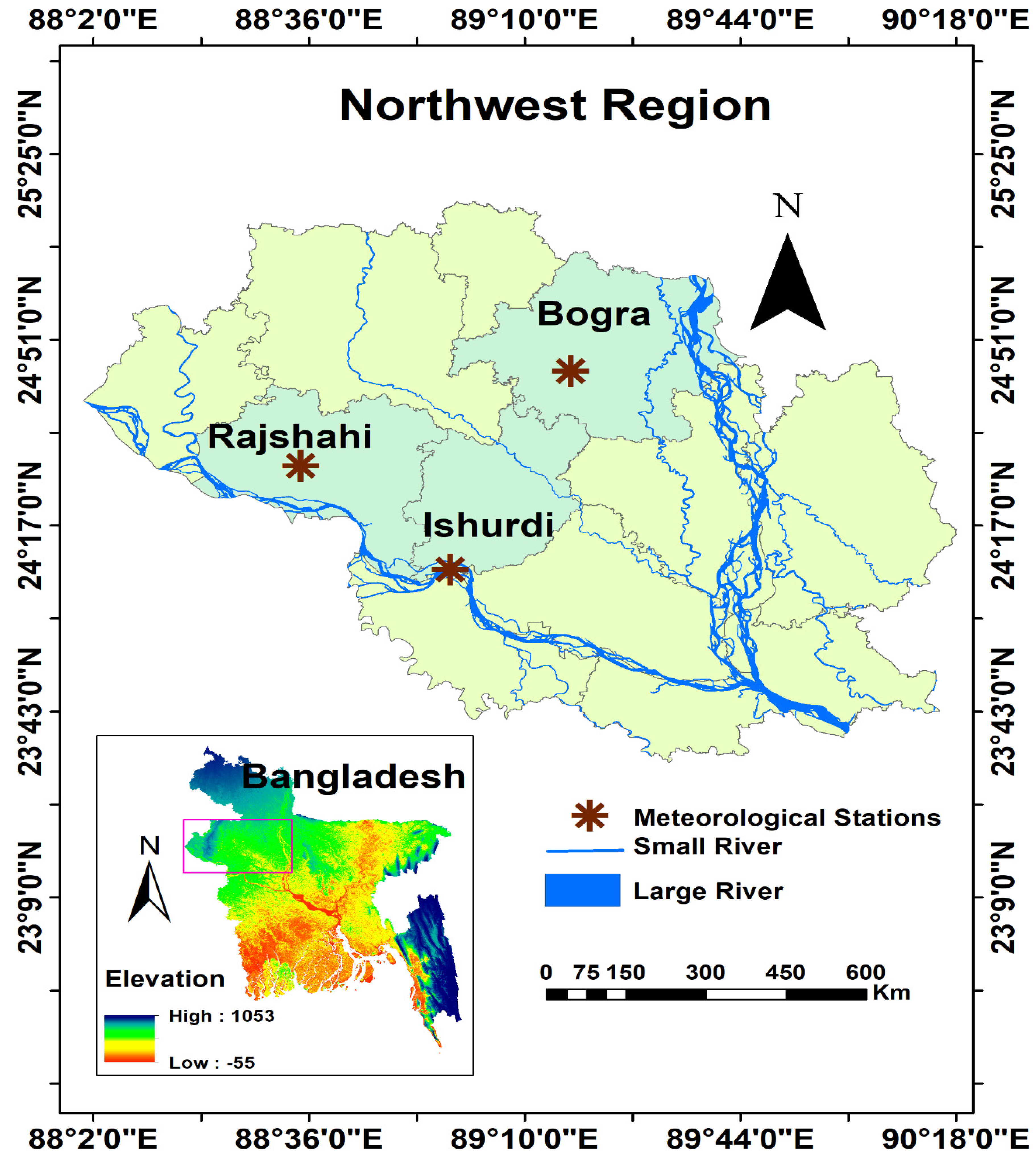
The study area is situated in the northwest region of Bangladesh as shown in Figure 1 (24.08° N to 25.13° N latitude and from 88.01° to 89.10° E longitude). The study region is a part of the Barind Tract, distributed mainly in the greater districts of Rajshahi, Bogra, and Pabna, which have a gross area of 7727 km2 [39]. Bangladesh has a subtropical monsoon climate with large spatial and temporal variability. It has four different seasons (e.g., pre-monsoon, monsoon, post-monsoon, and winter). In 85% of the country, annual rainfall occurs in the monsoon period. Less than 6% of rainfall occurs in the winter period. In the northwest, the annual mean total rainfall is 1329 mm [40]. In the winter season, the mean temperature varies between 17 and 20.6 °C while in the post-monsoon, it ranges from 26.9 to 31.1 °C. The Bangladesh Meteorological Department (BMD) reported that the temperature in pre-monsoon increases to 45 °C and the temperature in winter falls at 5 °C in the northwest part of the study area [41]. The northwest region experiences extreme events such as drought more frequently than the remaining parts of the country.
The northwest region has faced recurrent mean rainfall of more than 70 mm in the last 30-year period. The northwest part experiences an irregular rainfall distribution that makes this region desertified. However, this portion has fewer variations in regard to temperature. The study region also has a higher altitude compared to the rest of the country. This region faces natural hazards such as floods, drought, and tornadoes. Bangladesh was selected as the case study country because many drought events have happened in this region in recent years. This region faces a severe drought once every 2.5 years [42]. In the selected country, the northwest region was specifically selected for this study due to the fact that most drought events occur because of irregular rainfall distribution that causes intense variations in the region’s climate [43]. In addition to high fluctuations in rainfall patterns, this region is also drier than other parts of the country due to its lower mean precipitation compared to other parts of the country. Sandy soil properties reduce the soil moisture-holding capacity with an enhancement in the infiltration rate [43]. The abovementioned points compelled us to choose and analyze this region in this study for drought modeling.
2.2. Standard Precipitation Index (SPI)
The precipitation assessment is a complex procedure because of its spatiotemporal variability. As a result, an appropriate drought index must be adopted, and SPI is the most suitable and popular tool. SPI is a meteorological drought index with diverse time scales, e.g., 1, 3, 6 months for short-term and 9, 12, and 24 months for a long-term period. SPI is a suitable computing method for diverse drought phenomena [44]. Each time scale can be utilized for a specific intention [42]. Monthly precipitation datasets should perform for a specific period [45]. SPI mathematically relies on the cumulative likelihood of the observed precipitation dataset, which has confirmed that the precipitation exhibits the gamma probability density function (PDF) [46]. Computing a period of precipitation as a random variable x, the probability density of the Γ distribution is:
Among them, β > 0, γ > 0 are the scale and shape parameters, respectively; β and γ can be obtained by the maximum likelihood estimation method:
In the formula, xi is the precipitation data sample; is the average precipitation value. G(x) is obtained by integrating the probability density function g(x) of I then completing the gamma distribution. The accumulated value under the time scale is:
where x refers to the precipitation over a given time scale (mm); G(x) indicates the cumulative probability (CP) corresponding to x. The Gamma function is not defined for x = 0. For that reason, the distribution of precipitation may hold zeros and the CP is:
where q is the probability of a zero. Then, SPI can be computed by the following formula:
where c0 = 2.515517; c1 = 0.802853; c2 = 0.010328; d1 = 1.432788; d2 = 0.189269; d3 = 0.001308 (McKee et al., 1993). Classification of drought based on SPI can be obtained from the past studies [47,48].
2.3. Random Vector Functional Link Networks (RVFL)
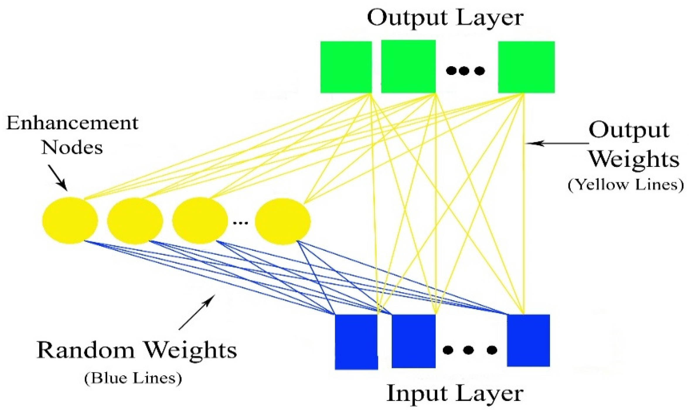
The Random Vector Functional Link (RVFL) networks of the input pattern accomplishes a non-linear transformation before feeding into the network’s input layer, which generates an enhanced pattern [49]. The RVFL is a type of Single Layer Feedforward Neural Network (SLFNN), containing a connection between the input and output layers, as shown in Figure 2. This link prevents the over-fitting problem, which is common in traditional SLFNN. The primary role of a functional link is to try to extend a feature space, which can induce an anticipated function. The RVFL obtains the Ns sample data (X), characterized as a pair (xi, yi), where yi is the goal variable. The input data are processed through the middle (hidden) nodes afterward. These middle nodes are called nodes of enhancement. Each middle node’s output is computed as below:
where βj indicates the weights between the input layer nodes and the enhancement (middle) nodes, and αj refers to the bias. S refers to the scale factor and is evaluated throughout the optimization procedure. The formula below computes the outcomes of RVFL:
where W refers to the weight of the output and F indicates a matrix consisting of the input samples F1 and the outcome of middle layer F2:
The above-mentioned equations are followed by updating the output weight via the below equations, which, respectively, indicate the Moore–Penrose pseudo-inverse and ridge regression:
where C is a trading-off parameter and is the Moore–Penrose pseudo-inverse.
2.4. Particle Swarm Optimization (PSO)
PSO is a type of population-based stochastic optimization algorithm. The PSO begins by producing the population called a swarm, i.e., particles. The corresponding positions of the particles show the possible solutions to the optimization process. Each particle in this method has a main characteristic, i.e., velocity [50]. The equations shown below state the position and the velocity for a provided particle i at epoch t, respectively.
where n is the quantity of parameters. Each particle’s position and velocity requires iteratively updating as below:
where, t + 1, t, vi,t, and xi,t represent the next and the current iterations, the velocity, and the position of the particle i at iteration t, respectively. pbesti,t and gbesti,t then are the individual’s best previous and global position i. Moreover, c1 and c2 are the learning rates that indicate the influence of the social and cognitive components and r1 and r2 are arbitrarily selected numbers that vary between 0 and 1. Eventually, X is a convergence factor and is usually considered to be about 0.729 [51].
The final step of the searching process in PSO is the updating of the best position and the determination of the best individual in the entire swarm for the individual i. To minimize the problem, the below equations should be utilized.
Two basis functions with a range of inputs define the other variable. The variable Y, mapped from the variable X with c as the threshold, is given below.
where f refers to the objective function. Overall, the abovementioned steps will be repeated until the considered criterion is satisfied.
2.5. Genetic Algorithm (GA)
Since its development by Holland [52], GA has been accepted as an influential search algorithm and a conventional optimization method. It was inspired by natural genetics [53]. It begins the same as the other optimization methods. However, this algorithm varies from other similar optimization methods. This method permits an evolution in population, composed of numerous individuals under determined rules, and minimizes the objective function. At the same time, selection, crossover, and mutation are the three major processes of this method. The main steps of GA have been stated briefly below. The GA has control parameters, a population size, (n)-generally varies from 20 to 100, the crossover rate generally varies from 0.7 to 1, and the mutation rate generally varies from 0.01 to 0.05 [54].
An initial population of decision variables, called ‘strings’, is first randomly generated. The ‘’fitness’’ of the searching string of the population is then evaluated, taking into account the constraints and objective function. The linearly sorted strings are then mapped to a ranking fitness value: the highest and lowermost mating probability. There is a mating pool in this step, and the chosen string is assigned a mating partner within it. After determining the string pairs to mate, the crossover is applied to exchange information between two-parent strings. This results in the generation of children’s strings. The population size is set at a constant or the same within the generations by exchanging the strings of parents and new children. Some alleles situated on the strings are randomly muted to not allow premature convergence to a local minimum. The procedure of mutation, selection, and crossover is repeated until a stopping criterion is satisfied.
2.6. Grey Wolves Optimization (GWO)
GWO is a kind of population-based metaheuristic algorithm introduced by Mirjalili et al. [55]. It was developed from the strategy of hunting and leadership skills and the hunting strategy of grey wolves.
In this method, a set of possible solutions is randomly generated. Each solution indicates one wolf, and the set shows the population of wolves in that problem. The generated population, then, is divided into four groups, considering their level of decision making in the hunting process: alpha (α), beta (β), delta (δ), and omega (ω). α, β, and δ wolves correspond to the first three fittest wolves, correspondingly, and lead other groups (ω) toward better solutions.
Then, the next step, the circling process around the target, is completed. This step can be stated as below:
where t is the current iteration, while t + 1 is the next iteration. Xp(t) is the target vector which is likely to be the position of the wolf α. D and A are calculated as below:
where, C = 2r2, X (t) shows the grey wolf situation; α is usually reduced linearly from 2 to 0; r1 and r2 are random vectors from 0 to 1. Considering the positions of wolves α, β, and δ, the group ω changes its location according to the below equation:
where X1, X2, X3 are calculated as follows:
where Xα, Xβ, and Xδ correspond to α, β, and δ positions, respectively. Moreover, Dα, Dβ, and Dδ are evaluated as below:
A = 2α·r1 − α
C1, C2, and C3 are random vectors, while X(t) depicts the current solution. When the abovementioned steps are completed, the corresponding fitness value is calculated, and the best solution is assumed to be α. This step keeps going to satisfy the stopping criterion, where GWO is ended.
2.7. Social Spider Optimization (SSO)
The SSO algorithm proposed by Cuevas et al. [56] was inspired by particle swarm optimization. It imitates the social intellect of spiders living in a colony. They utilize vibrations throughout the web for communication. Therefore, the search space and agents are assumed as the web and spiders, respectively. In the present algorithm, the agents are categorized into males (M) and females (F). Each spider’s weight is assumed as its fitness. The SSO algorithm assumed that females in spider colonies are more than males, representing more than 60% of the population. Vibrating the strings of the web is how spiders communicate, which reveals the size and distance of the message sender. The proposed model by Cuevas et al. [51] is as below:
where α, β, δ, and r, are random values between 0 and 1. In addition, Sc and Sb show the best closest neighbor and the fittest spider in the population, correspondingly. The procedure allowing the male spider to update in position varies from the females. The males here are divided into dominated (D) and non-dominated (ND). The mathematical expression of the before-mentioned categories, i.e., ND and D-type males, is as below:
where Sf is the closest female to ith male, and α, δ, and rare random values in [0, 1]. The mating operator, which modifies the search agents, is the last tool of SSO. ND males need to meet females in a distinct area around them, called the mating radius. There may be more than one pair of males and females in the mating radius, and the fitness of pairs, therefore, is essential in their selection. Producing the new generation is the next step after the mating process. The new generation fitness, then, is checked. If it is better than the worst spider in population, the new generation will be saved, and the worst will be removed. The abovementioned process is iterated until the constraints are satisfied.
2.8. Salp SWARM Algorithm (SSA)
Mirjalili et al. [57] proposed the SSA method in 2017 as a population-based optimization method. There are two groups of individuals (Salps) in SSA, and their positions in the chain are as leaders or followers. The leader is the first individual of the chain, and the others are followers who the leader guides in their movement.
Initializing the salp population is the first step of SSA, which can be seen in the below equation as a two-dimensional matrix:
The fitness of each salp, then, is evaluated to determine the leader (i.e., the salp with the best fitness). The leader’s position is updated as below:
where , yi, lbi, and ubi are the first salp, food position, the lower bound, and the upper bound of the ith dimension, respectively. The coefficient r1 is also calculated as below, while r2 and r3 are random numbers between 0 to 1:
where L and l are the maximum and current iterations, respectively. Followers, moreover, need to update their positions, which can be calculated as below:
where j ≥ 2 denotes the position of the jth salp in the ith dimension, while δ0 and t are initial speed and time:
If some salps move outside of the search space, the equation below will bring them back to the search space.
2.9. Hunger Games Search (HGS)
HGS is a novel population-based optimization technique proposed by Yang et al. [38]. The hunger-driven activities and behavioral choices of animals were the basis of the development of HGS, as it follows a notion of “Hunger”. Hunger is the most vital reason for a broad domain of actions in an animal’s life. Indeed, the HGS method simulates the consequence of hunger on each search step. The higher chances of survival and food gain are the basis of the HGS algorithm. Collaboration in hunting is common for social animals. Still, there is always the possibility that some of them will not participate in a group foraging process [58,59].
The main idea of the HGS can be understood in the below equation, where the cooperative nature of animal communication and hunting can be modeled as:
where r1 and r2 are random numbers in the range of [0, 1]. randn (1) is a random number and satisfies normal distribution. t shows the existing iterations. and indicate the weights of hunger. Moreover, and show the location of the best separate iteration and each individual’s location, respectively. (1 + randn (1)) represents the random food search by a hungry agent at a current location. The range of individual activity can be modeled at present. When is multiplied by , the result can show the effect of hunger on the activity range. is a ranging controller that limits the activity range and slowly decreases to 0. E can be formulated as below:
where i ∈ 1, 2, …, n; F(i) and BF are the fitness value of each individual and the best fitness obtained in the current iteration process so far, respectively. Moreover, sech is a hyperbolic function (sech (x) = 2ex + e − x).
E = sech (|(i) − BF |)
The HGS simulates the hunger features of individuals in mathematical searches. Based on the main equation of HGS, and can be calculated as below:
where Hungry and SHungry are the starvation of each individual and the number of hungry feelings of all individuals, respectively. N is the number of individuals, while (Hungry); r3, r4, and r5 are random numbers in the range of [0, 1]. hungry (i), therefore, can be evaluated as below:
where AllFitness (i) conserves the fitness of each individual in the present iteration. H is added for the other individuals, based on the original hunger, and is evaluated by the equation shown below:
where r6 is a random number between 0 and 1; WF indicates the worst fitness gained in the current iteration so far; and UB and LB are the upper and lower bounds of the feature space, respectively. The hunger sensation H is limited to a lower bound, LH, to allow the algorithm to obtain a better performance [60].
2.10. Model Performance Evaluation Matrices
Monthly precipitation data from three stations in Bangladesh were used to calculate SPI3, SPI6, SPI9, and SPI12 indices, and the methods were compared using the statistical indices expressed below:
where separately refer to the computed, observed mean of the observed SPI and data number.
3. Application and Results
This section presents and compares the outcomes of the several hybrid RVFL methods tuned with PSO, GA, GWO, SSO, SSA, and HGS in forecasting drought based on SPI. The control parameter information is reported in Table 1 for each algorithm. Data were split into 80–20% for training and test sets. Several control parameters provided in Table 1 were tried for the applied models and algorithms. Population and iteration numbers were set to 40 and 100 for all algorithms. To obtain robust outcomes, each algorithm was run 20 times.
The RFVL-based models are compared in forecasting SPI3 and SPI6 drought indices for the first and third stations in Tables S1 and S2, respectively. Optimal input combinations were decided to account for correlation analysis (partial auto-correlation function) for each index. For example, in Table S1, SPI3t-1 input was used to forecast SPI3t, which indicates the SPI3 value at the current month. As seen from Tables S1 and S2, models with the first input combination (SPI3t-1) provided the best accuracy in forecasting SPI3. In contrast, the second input scenario (SPI6t-1, SPI6t-2, SPI6t-3, SPI6t-4) produced the best models in forecasting SPI6 in the first and second stations. It is clear from Table 1 that the hybrid RFVL models outperformed the single RFVL and the RFVL–HGS had the best accuracy in forecasting droughts based on SPI3 and SPI6 (RMSE = 0.489, MAE = 0.337, R2 = 0.815 and NSE = 0.752 for SPI3 and RMSE = 0.430, MAE = 0.275, R2 = 0.829 and NSE = 0.782 for SPI6) in station 1. The HGS algorithm considerably improved the accuracy of the single RFVL in forecasting SPI3 (improvement in RMSE, MAE, R2, and NSE by 6.14, 7.67, 7.52 and 9.62%) and SPI6 (improvement in RMSE, MAE, R2, and NSE by 11.89, 8.64, 8.94 and 16.20%, respectively).
Similar to the first station, in the second station (Table 2), the HGS also decreased the RMSE and MAE of the single RFVL from 0.548 and 0.371 to 0.515 and 0.351 and increased the R2 and NSE from 0.764 and 0.727 to 0.814 and 0.785 in forecasting SPI3. In contrast, the RMSE, MAE, R2, and NSE improvements of the single RFVL were 17.42, 26.40, 9.51 and 15.44% in forecasting SPI6, respectively. In the third station (Table S2), applying HGS in tuning RFVL improved its accuracy by reducing RMSE and MAE from 0.570 and 0.409 to 0.511 and 0.340 by 7.55 and 10.87% and increasing R2 and NSE from 0.705, and 0.647 to 0.769 and 0.734 by 6.52 and 9.05% in forecasting SPI3, whereas the improvements in RMSE, MAE, R2 and NSE of the single RFVL were 26.45, 27.40, 9.56 and 13.26% in forecasting SPI6, respectively. The relative RMSE differences between the HGS and other algorithms (PSO, GA, GWO, SSO, SSA), respectively were 6.14, 4.86, 4.49, 4.12, 2.59 and 2.20% in forecasting SPI3 of station 1 while the corresponding values were 11.89, 4.02, 2.49, 2.27, 1.60 and 0.69% for SPI6. In the other two stations, the differences were also similar. These show that the accuracy ranks of the algorithms were (from the best to the worst): HGS > SSA > SSO > GWO > GA > PSO in forecasting SPI3 and SPI6.
Tables S3 and S4 sum up the training and test statistics of the RFVL-based models in forecasting the SPI9 and SPI12 drought indices of first and third stations, respectively. However, the results of station 2 are listed in Table 3. In all stations, the hybrid RFVL models had a superior performance compared to the single RFVL in forecasting SPI9 and SPI12 drought indices. In the first and third stations (Tables S3 and S4), all models provided the best accuracy for the first input combination, including three previous SPI values as inputs to the models (e.g., SPI9t-1, SPI9t-2, SPI9t-3) in forecasting SPI9. In contrast, the best SPI12 forecasts were obtained from the second input combination (SPI12t-1, SPI12t-2, SPI12t-3, SPI12t-4, SPI12t-5). Tuning RFVL parameters by HGS considerably improved its accuracy in forecasting SPI9 (improvement in RMSE, MAE, R2, and NSE by 14.14, 14.53, 10.31 and 11.78%) and SPI12 (improvement in RMSE, MAE, R2, and NSE by 24.50, 30.68, 18.70 and 25.11%, respectively). Unlike the first and third stations, in the second station (Table 3), all models performed the best for the first input combination in forecasting SPI9 and SPI12. In the case of SPI9 forecasting, the RMSE and MAE of the single RFVL decreased from 0.430 and 0.291 to 0.372 and 0.260, and R2 and NSE increased from 0.788 and 0.760 to 0.838 and 0.823 by implementing HGS for training. Similarly, the improvement in the accuracy of the single RFVL in forecasting SPI12, respectively, was 24.86, 27.40, 11.98 and 12.47% concerning the application of the HGS algorithm in training.
In the third station, the RFVL tuned with HGS had the lowest RMSE and MAE and the highest R2 and NSE in forecasting SPI9 (RMSE = 0.333, MAE = 0.137, R2 = 0.873 and NSE = 0.849) and SPI12 (RMSE = 0.276, MAE = 0.114, R2 = 0.893 and NSE = 0.880). Implementing HGS as a training algorithm considerably improved the forecasting accuracy of a single RFVL; the improvements obtained for RMSE, MAE, R2, and NSE were 15.27, 29.02, 9.81 and 8.99% for SPI9 and the corresponding percentages for SPI12 were 13.21%, 26.92, 7.20 and 9.18% for SPI12, respectively. The relative RMSE differences between HGS and other algorithms (PSO, GA, GWO, SSO, SSA), respectively, were 14.14, 13.79, 12.91%, 11.27, 4.92 and 1.85% in forecasting SPI9 of station 1 while the corresponding values were 24.50, 7.34, 5.25, 4.77, 2.82 and 2.32% for SPI12. This rank was also the same in the other two stations, and the accuracy ranks of the algorithms in forecasting SPI9 and SPI12 were (from the best to the worst): HGS > SSA > SSO > GWO > GA > PSO. It can be seen from Table 1, Table 2 and Table 3 and Tables S3 and S4 (see the training results) that hybrid algorithms improved the approximation (fitting) accuracy of the single RFVL method in simulating drought indices, and the HGS had the first rank among the six algorithms. The HGS improved the RFVL accuracy with respect to RMSE by 14.09, 23.14, 15.42 and 21.52% for SPI3, SPI6, SPI9, and SPI12 in station 1, by 14.20, 25.62, 22.28 and 25% in station 2, and by 10.57, 23.24, 24.54 and 23.21% in station 3, respectively.
The effect of periodicity was also investigated by importing month numbers as inputs to the best-implemented models, and the outcomes are reported in Table 4 for the three stations using their SPI3 index. For example, OPT SPI3 + MN indicates the optimum SPI3 inputs (SPI3t-1 in our study, see Table 2) plus the month number. For SPI6, SPI 9, and SPI12, the estimations using the optimal input combinations of all stations with periodicity are reported in Tables S5–S7. It can be observed from the tables that periodicity mostly improved the models’ performances. For example, including MN in inputs improved the RMSE of RFVL, RFVL–PSO, RFVL–GA, RFVL–GWO, RFVL–SSO, RFVL–SSA, and RFVL–HGS by 0.38, 2.7, 2.73, 2.75, 2.19, 2.60 and 1.43%, respectively for forecasting SPI3, and the corresponding values were 2.66, 2.68, 2.27, 3.64, 5.49, 6.24 and 6.74% for forecasting SPI6.
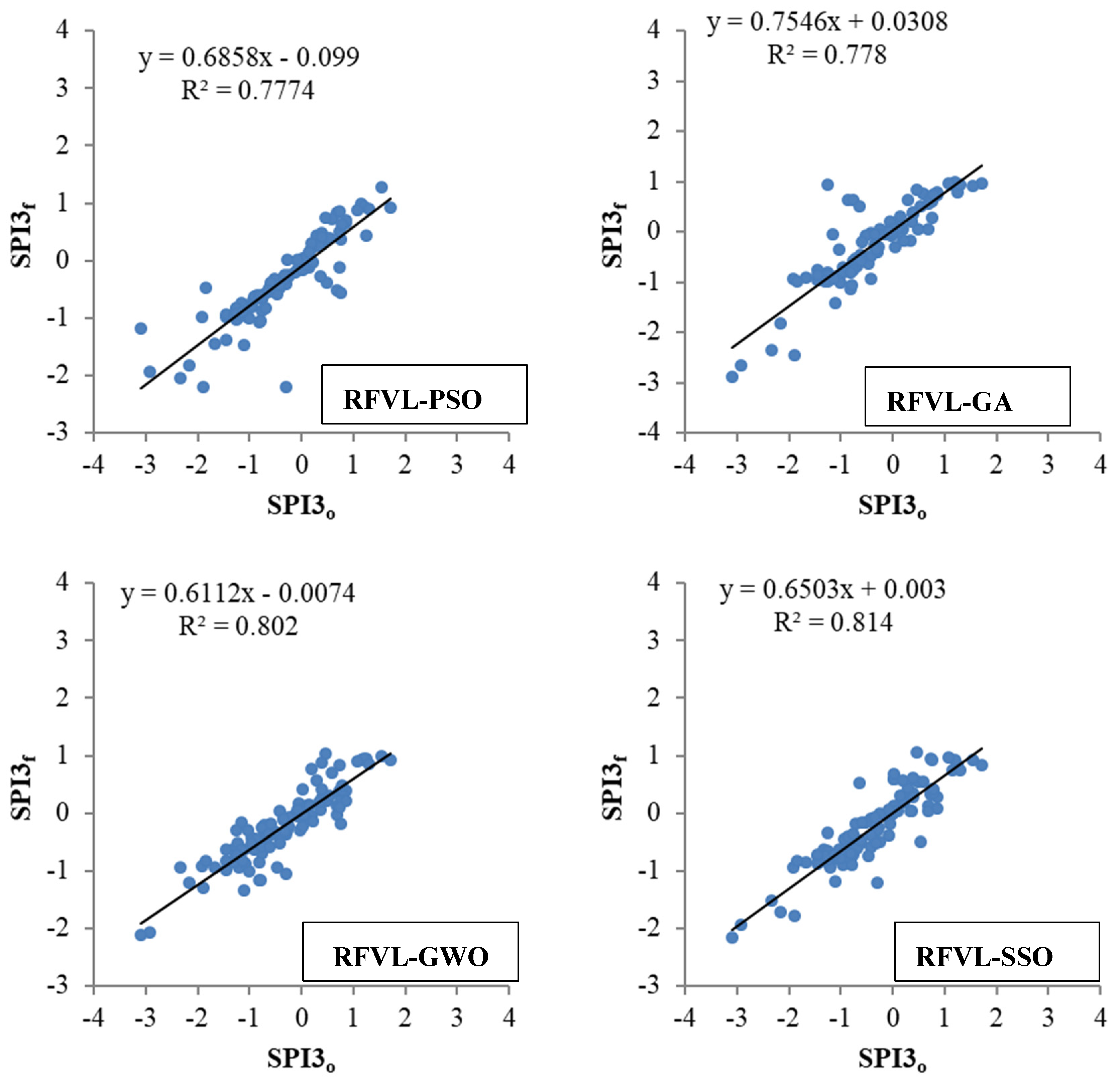
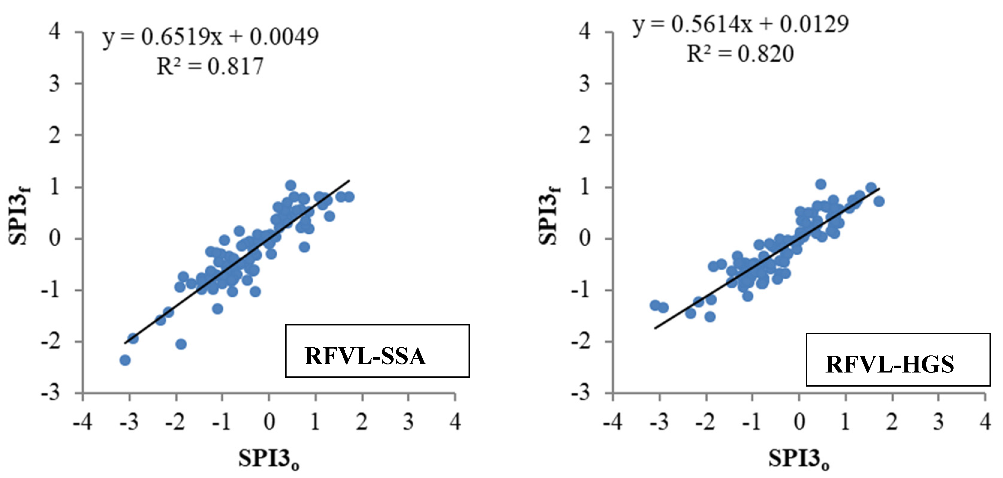
For example, the RFVL-based models are compared on scatter diagrams in Figure 3 in forecasting drought based on SPI3 and using the optimal inputs and the periodicity component (MN) for station 2. Among the metaheuristic algorithms, HGS seemed to have the least scattered forecasts in the test stage. At the same time, the PSO provided more scattered SPI3 values than the other algorithms. Similarly, the hybrid RFVL-based models are compared in Figures S1–S3 in forecasting SPI6, SPI9, and SPI12, respectively. As evident from the graphs, the RFVL–HGS provided the best forecasts with the lowest scattering. The RFVL–SSA and RFVL–SSO followed, and the RFVL-PSO had the worst accuracy in forecasting drought based on the SPI6, SPI9, and SPI12.
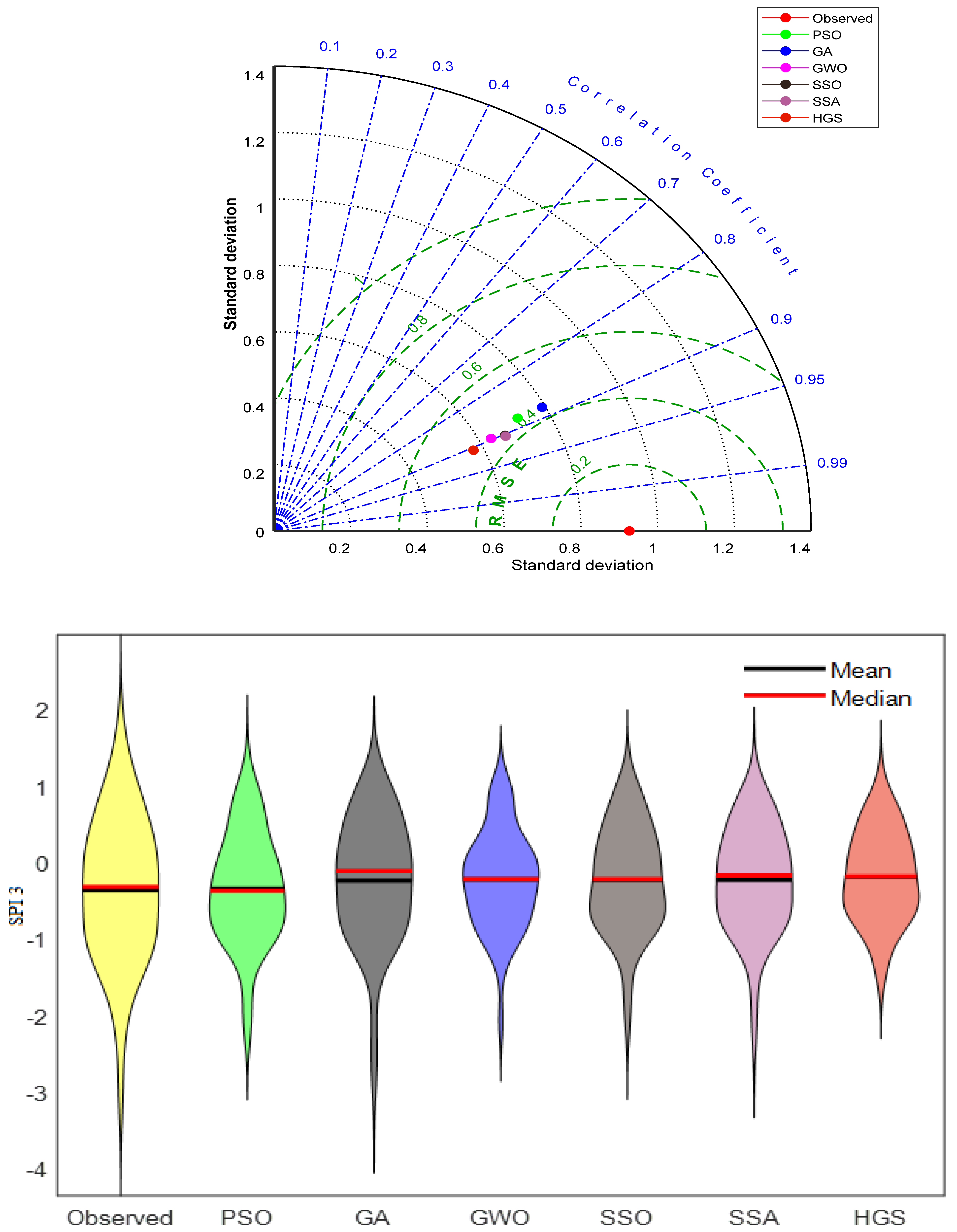
Figure 4 compares the drought forecasting accuracies of the RFVL-based models based on the SPI3 index using the Taylor and violin charts. Similarly, the Taylor and violin charts of the hybrid RFVL-based models are compared in Figures S4–S6 in forecasting SPI6, SPI9, and SPI12, respectively. It can be seen from the Taylor charts that HGS had a closer standard deviation to the observed one compared to other algorithms, and it had the lowest RMSE and the highest correlation. The violin charts show that the drought forecasts of the HGS-based RFVL provided a closer distribution to the observed one than other alternatives. The assessment criteria and visual inspections tell us that the metaheuristic algorithms considerably improved the accuracy of the RFVL method in forecasting drought based on SPI indices. Among the algorithms, the HGS had the best efficiency. The main advantage of the population-based HGS method is its stochastic switching elements, which enriches its exploratory and exploitative behavior. It has a high efficiency in handling multi-modality and local optima problems because it has an adaptive and time-varying mechanism [36].
4. Discussion
The study outcomes revealed that combining hybrid algorithms improves the accuracy of a single RVFL method in forecasting drought based on SPI3, SPI6, SPI9, and SPI12. This is in line with the previous study [61,62], which reported that the hybridized version of the machine learning methods has a better prediction accuracy and a better predictive power. The HGS algorithm considerably improved the accuracy of the single RFVL in forecasting SPI3, SPI6, SPI9, and SPI12 in all three stations. The assessment criteria and visual inspections tell us that the metaheuristic algorithms considerably improved the accuracy of the RFVL method in forecasting drought based on SPI indices. All these new algorithms (metaheuristic algorithms) have advantages over traditional ones which have problems tackling local optima in optimization. Due to the limitations of the standard RFVL, a considerable improvement is obtained by tuning it with metaheuristic algorithms. The HGS had the best efficiency among the implemented algorithms. The main advantage of the population-based HGS method is its stochastic switching elements, which enriches its exploratory (exploration can be defined as the procedure of visiting entirely new regions of a searched space) and exploitative (exploitation is defined by the procedure of visiting those regions of a searched space within the neighborhood of previously visited points) behavior [63]. It has a high efficiency in handling multi-modality and local optima problems because it has an adaptive and time-varying mechanism [36].
The results showed that the periodicity mostly improved the models’ accuracy in drought forecasting (e.g., the improvement in RMSE of RVFL and RVFL–HGS was 0.38% and 1.43% for SPI3 and 2.66% and 6.74 for SPI6, respectively). This finding is directly in line with the previous literature [64,65]. Kisi [64] and Adnan et al. [65] indicated that adding periodicity to the model inputs improved the accuracy of the least square support vector regression (LSSVR), the feed-forward neural network (FFNN), the radial basis neural network (RBNN), the generalized regression neural network (GRNN), and the adaptive neuro-fuzzy inference system (ANFIS) in forecasting streamflows.
In a study implemented by Belayneh and Adamowski [66], the viability of wavelet neural networks (WNN)to forecast SPI-3 and SPI-12 was investigated. The best models produced R2 of 0.780 and 0.908. The study conducted by Jalalkamali et al. [67] examined the accuracy of three methods, MLP, ANN, and ANFIS, in forecasting SPI-3, SPI-6, and SPI-9. They found R2 of 0.801, 0.774, and 0.706 for the optimal models, respectively. The study of Kisi et al. [25] investigated the performances of the ANFIS hybridized with metaheuristic methods in forecasting SPI indices. The best models produced R2 of 0.760, 0.850, 0.771, and 0.832 for the SPI-3, SPI-6, SPI-9, and SPI-12, respectively. Recently, in a study performed by Gorgij et al. [68], the efficiency of four methods, long short-term memory (LSTM), extra-trees (ET), the vector autoregressive approach (VAR), and multivariate adaptive regression spline (MARS), was investigated in forecasting SPI-3, SPI-6, SPI-9, and SPI-12 in four stations. The NSE of the best model (LSTM) ranged from 0.682 to 0.697, 0.780 to 0.815, 0.777 to 0.848 and 0.852 to 0.904 for forecasting SPI-3, SPI-6, SPI-9, and SPI-12, respectively. The outcomes of this study reported in Tables S2–S7 indicate that the RVFL–HGS model can generate accurate drought forecasts based on the standard precipitation index.
5. Conclusions
In this study, to find an efficient drought forecasting method, six different hybrid RFVL methods tuned with PSO, GA, GWO, SSO, SSA, and HGS algorithms, were compared, using four SPI indices, including SPI3, SPI6, SPI9, and SPI12. SPI indices were calculated from monthly precipitation data acquired from three stations located in northwest Bangladesh. The comparison of the methods was assessed based on RMSE, MAE, R2, NSE, and visual inspections, including scatter plots, and Taylor and violin charts. The metaheuristic algorithms improved the accuracy of the single RFVL in the simulation (training stage) and forecasting (testing stage) drought based on SPI3, SPI6, SPI9, and SPI12. Among the algorithms, the HGS provided the best performance by improving the RMSE accuracy of RFVL by 6.14, 11.89, 14.14 and 24.5% in forecasting the SPI3, SP6, SPI9, and SPI12 in station 1, by 6.02, 17.42, 13.49 and 24.86 in station two and by 7.55, 26.45, 15.27 and 13.21 in station 3, respectively. The HGS also increased the forecasting accuracy of the RVFL-based PSO, GA, GWO, SSO, SSA in forecasting SPI3, SPI6, SPI9, and SPI12.
Including the periodicity component in the models’ inputs generally improved the accuracy of the RFVL-based methods in forecasting drought based on four SPI indices. The improvement with respect to RMSE statistics ranged from 0.38 to 2.75%, 2.27 to 6.74%, 5.75 to 16.4% and 9.93 to 10.5% for the SPI3, SPI6, SPI9, and SPI12, respectively. The accuracy comparison of the algorithms revealed that the accuracy ranks of the algorithms were, in descending order (from the best to the worst): HGS > SSA > SSO > GWO > GA > PSO in forecasting SPI3, SPI6, SPI9, and SPI12. According to the results of this study, the use of HGS-based RVFL is recommended for drought modeling. Thus, the presented method can be useful for decision-makers in mitigating the effects of drought and providing effective plans for water resource management.
The main limitation of this study was use of data from only three stations in northwest Bangladesh to test the implementation of the methods. The study could be extended by testing these methods using more data from other regions. Future studies could compare the investigated algorithms and methods with other metaheuristic algorithms and/or methods.
Supplementary Materials
The following are available online at https://www.mdpi.com/article/10.3390/w13233379/s1, Figure S1. Scatterplots of the observed and predicted SPI6 drought index by different RFVL based models in the test period –Station 2, Figure S2. Scatterplots of the observed and predicted SPI9 drought index by different RFVL based models in the test period–Station 2, Figure S3. Scatterplots of the observed and predicted SPI12 drought index by different RFVL based models in the test period–Station 2, Figure S4. Taylor and Violin diagrams of SPI6 drought index by different RFVL based models in the test period–Station 2, Figure S5. Taylor and Violin diagrams of SPI9 drought index by different RFVL based models in the test period–Station 2, Figure S6. Taylor and Violin diagrams of SPI12 drought index by different RFVL based models in the test period–Station 2. Table S1. The comparison of different RFVL based models in forecasting SPI3 and SPI6 drought indices–Station 1, Table S2. The comparison of different RFVL based models in forecasting SPI3 and SPI6 drought indices–Station 3, Table S3. The comparison of different RFVL based models in forecasting SPI9 and SPI12 drought indices–Station 1, Table S4. The comparison of different RFVL based models in forecasting SPI9 and SPI12 drought indices–Station 3, Table S5. The comparison of different RFVL based models in SPI6 drought estimation for the test period using Periodicity with optimal inputs, Table S6. The comparison of different RFVL based models in SPI9 drought estimation for the test period using Periodicity with optimal inputs, Table S7. The comparison of different RFVL based models in SPI12 drought estimation for the test period using Periodicity with optimal inputs.
Author Contributions
Conceptualization: R.M.A., O.K., A.D.G. and A.R.M.T.I. Formal analysis: A.K., O.K. and R.R.M. Validation: R.M.A., A.K., A.D.G., A.R.M.T.I. and O.K. Supervision: O.K. and A.R.M.T.I. Writing original draft: R.M.A., A.K., A.D.G., O.K., A.R.M.T.I. and R.R.M. Visualization: R.M.A., A.K., R.R.M. and A.D.G. investigation: R.M.A., A.K. and A.D.G. All authors have read and agreed to the published version of the manuscript.
Funding
No Funding Received.
Institutional Review Board Statement
Not applicable.
Informed Consent Statement
Not applicable.
Data Availability Statement
The data presented in this study will be available on an interesting request from the corresponding author.
Conflicts of Interest
There is no conflict of interest in this study.
References
- Du, J.; Fang, J.; Xu, W.; Shi, P. Analysis of dry/wet conditions using the standardized precipitation index and its potential usefulness for drought/flood monitoring in Hunan Province, China. Stoch. Environ. Res. Risk Assess. 2013, 27, 377–387. [Google Scholar] [CrossRef]
- Palmer, W.C. Meteorological Drought; US Department of Commerce, Weather Bureau: Washington, DC, USA, 1965; Volume 30.
- Nicault, A.; Alleaume, S.; Brewer, S.; Carrer, M.; Nola, P.; Guiot, J. Mediterranean drought fluctuation during the last 500 years based on tree-ring data. Clim. Dyn. 2008, 31, 227–245. [Google Scholar] [CrossRef]
- Hanjra, M.A.; Qureshi, M.E. Global water crisis and future food security in an era of climate change. Food Policy 2010, 35, 365–377. [Google Scholar] [CrossRef]
- Mancosu, N.; Snyder, R.L.; Kyriakakis, G.; Spano, D. Water Scarcity and Future Challenges for Food Production. Water 2015, 7, 975–992. [Google Scholar] [CrossRef]
- Hao, Z.; AghaKouchak, A.; Nakhjiri, N.; Farahmand, A. Global integrated drought monitoring and prediction system. Sci. Data 2014, 1, 140001. [Google Scholar] [CrossRef]
- Santos, C.A.G.; Brasil Neto, R.M.; da Silva, R.M.; dos Santos, D.C. Innovative approach for geospatial drought severity classification: A case study of Paraíba state, Brazil. Stoch. Environ. Res. Risk Assess. 2019, 33, 545–562. [Google Scholar] [CrossRef] [Green Version]
- Spinoni, J.; Vogt, J.V.; Naumann, G.; Barbosa, P.; Dosio, A. Will drought events become more frequent and severe in Europe? Int. J. Climatol. 2017, 38, 1718–1736. [Google Scholar] [CrossRef] [Green Version]
- Hao, Z.; Singh, V.P.; Xia, Y. Seasonal Drought Prediction: Advances, Challenges, and Future Prospects. Rev. Geophys. 2018, 56, 108–141. [Google Scholar] [CrossRef] [Green Version]
- Svoboda, M.; LeComte, D.; Hayes, M.; Heim, R.; Gleason, K.; Angel, J.; Rippey, B.; Tinker, R.; Palecki, M.; Stooksbury, D.; et al. The drought monitor. Bull. Am. Meteorol. Soc. 2002, 83, 1181–1190. [Google Scholar] [CrossRef] [Green Version]
- Feng, X.; Ackerly, D.D.; Dawson, T.E.; Manzoni, S.; Skelton, R.P.; Vico, G.; Thompson, S.E. The ecohydrological context of drought and classification of plant responses. Ecol. Lett. 2018, 21, 1723–1736. [Google Scholar] [CrossRef] [PubMed] [Green Version]
- Moreira, E.E.; Coelho, C.A.; Paulo, A.A.; Pereira, L.S.; Mexia, J.T. SPI-based drought category prediction using loglinear models. J. Hydrol. 2008, 354, 116–130. [Google Scholar] [CrossRef] [Green Version]
- AghaKouchak, A. A multivariate approach for persistence-based drought prediction: Application to the 2010–2011 East Africa drought. J. Hydrol. 2015, 526, 127–135. [Google Scholar] [CrossRef]
- Kumar, M.N.; Murthy, C.S.; Sai, M.V.R.S.; Roy, P.S. On the use of Standardized Precipitation Index (SPI) for drought intensity assessment. Meteorol. Appl. 2009, 16, 381–389. [Google Scholar] [CrossRef] [Green Version]
- Livada, I.; Assimakopoulos, V.D. Spatial and temporal analysis of drought in greece using the Standardized Precipitation Index (SPI). Theor. Appl. Clim. 2006, 89, 143–153. [Google Scholar] [CrossRef]
- Vicente-Serrano, S.M.; Beguería, S.; López-Moreno, J.I. A Multiscalar Drought Index Sensitive to Global Warming: The Standardized Precipitation Evapotranspiration Index. J. Clim. 2010, 23, 1696–1718. [Google Scholar] [CrossRef] [Green Version]
- Ribeiro, A.; Pires, C. Seasonal drought predictability in Portugal using statistical–dynamical techniques. Phys. Chem. Earth Parts A/B/C 2015, 94, 155–166. [Google Scholar] [CrossRef]
- Hosseini-Moghari, S.M.; Araghinejad, S. Monthly and seasonal drought forecasting using statistical neural networks. Environ. Earth Sci. 2015, 74, 397–412. [Google Scholar] [CrossRef]
- AghaKouchak, A. A baseline probabilistic drought forecasting framework using standardized soil moisture index: Application to the 2012 United States drought. Hydrol. Earth Syst. Sci. 2014, 18, 2485–2492. [Google Scholar] [CrossRef] [Green Version]
- Poornima, S.; Pushpalatha, M. Drought prediction based on SPI and SPEI with varying time-scales using LSTM recurrent neural network. Soft Comput. 2019, 23, 8399–8412. [Google Scholar] [CrossRef]
- Mohamadi, S.; Sammen, S.S.; Panahi, F.; Ehteram, M.; Kisi, O.; Mosavi, A.; Ahmed, A.N.; El-Shafie, A.; Al-Ansari, N. Zoning map for drought prediction using integrated machine learning models with a nomadic people optimization algorithm. Nat. Hazards 2020, 104, 537–579. [Google Scholar] [CrossRef]
- Başakın, E.E.; Ekmekcioğlu, Ö.; Özger, M. Drought prediction using hybrid soft-computing methods for semi-arid region. Model. Earth Syst. Environ. 2021, 7, 2363–2371. [Google Scholar] [CrossRef]
- Deo, R.C.; Kisi, O.; Singh, V.P. Drought forecasting in eastern Australia using multivariate adaptive regression spline, least square support vector machine and M5Tree model. Atmos. Res. 2017, 184, 149–175. [Google Scholar] [CrossRef] [Green Version]
- Tosunoglu, F.; Kisi, O. Trend analysis of maximum hydrologic drought variables using Mann–Kendall and Şen’s innovative trend method. River Res. Appl. 2017, 33, 597–610. [Google Scholar] [CrossRef]
- Kisi, O.; Gorgij, A.D.; Zounemat-Kermani, M.; Mahdavi-Meymand, A.; Kim, S. Drought forecasting using novel heuristic methods in a semi-arid environment. J. Hydrol. 2019, 578, 124053. [Google Scholar] [CrossRef]
- Tao, H.; Al-Sulttani, A.O.; Ameen, A.M.S.; Ali, Z.H.; Al-Ansari, N.; Salih, S.Q.; Mostafa, R.R. Training and Testing Data Division Influence on Hybrid Machine Learning Model Process: Application of River Flow Forecasting. Complexity 2020, 2020, 8844367. [Google Scholar] [CrossRef]
- Alizamir, M.; Kisi, O.; Adnan, R.M.; Kuriqi, A. Modelling reference evapotranspiration by combining neuro-fuzzy and evolutionary strategies. Acta Geophys. 2020, 68, 1113–1126. [Google Scholar] [CrossRef]
- Yuan, X.; Chen, C.; Lei, X.; Yuan, Y.; Adnan, R.M. Monthly runoff forecasting based on LSTM–ALO model. Stoch. Environ. Res. Risk Assess. 2018, 32, 2199–2212. [Google Scholar] [CrossRef]
- Kisi, O.; Shiri, J.; Karimi, S.; Adnan, R.M. Three Different Adaptive Neuro Fuzzy Computing Techniques for Forecasting Long-Period Daily Streamflows. In Big Data in Engineering Applications; Springer: Singapore, 2018; pp. 303–321. [Google Scholar]
- Adnan, R.; Parmar, K.; Heddam, S.; Shahid, S.; Kisi, O. Suspended Sediment Modeling Using a Heuristic Regression Method Hybridized with Kmeans Clustering. Sustainability 2021, 13, 4648. [Google Scholar] [CrossRef]
- Malik, A.; Kumar, A. Meteorological drought prediction using heuristic approaches based on effective drought index: A case study in Uttarakhand. Arab. J. Geosci. 2020, 13, 1–17. [Google Scholar] [CrossRef]
- Banadkooki, F.B.; Singh, V.P.; Ehteram, M. Multi-timescale drought prediction using new hybrid artificial neural network models. Nat. Hazards 2021, 106, 2461–2478. [Google Scholar] [CrossRef]
- Adnan, R.M.; Mostafa, R.R.; Kisi, O.; Yaseen, Z.M.; Shahid, S.; Zounemat-Kermani, M. Improving streamflow prediction using a new hybrid ELM model combined with hybrid particle swarm optimization and grey wolf optimization. Knowl. Based Syst. 2021, 230, 107379. [Google Scholar] [CrossRef]
- Abraham, A.; Jain, R. Soft Computing Models for Network Intrusion Detection Systems. In Classification and Clustering for Knowledge Discovery; Halgamuge, S.K., Wang, L., Eds.; Springer: Berlin/Heidelberg, Germany, 2005; pp. 191–207. [Google Scholar]
- Fahim, S.R.; Hasanien, H.M.; Turky, R.A.; Alkuhayli, A.; Al-Shamma’A, A.A.; Noman, A.M.; Tostado-Véliz, M.; Jurado, F. Parameter Identification of Proton Exchange Membrane Fuel Cell Based on Hunger Games Search Algorithm. Energies 2021, 14, 5022. [Google Scholar] [CrossRef]
- Yang, Y.; Chen, H.; Heidari, A.A.; Gandomi, A.H. Hunger games search: Visions, conception, implementation, deep analysis, perspectives, and towards performance shifts. Expert Syst. Appl. 2021, 177, 114864. [Google Scholar] [CrossRef]
- Nguyen, H.; Bui, X.-N. A Novel Hunger Games Search Optimization-Based Artificial Neural Network for Predicting Ground Vibration Intensity Induced by Mine Blasting. Nat. Resour. Res. 2021, 30, 3865–3880. [Google Scholar] [CrossRef]
- AbuShanab, W.S.; Abd Elaziz, M.; Ghandourah, E.I.; Moustafa, E.B.; Elsheikh, A.H. A new fine-tuned random vector functional link model using Hunger games search optimizer for modeling friction stir welding process of polymeric materials. J. Mater. Res. Technol. 2021, 14, 1482–1493. [Google Scholar] [CrossRef]
- Zinat, M.R.M.; Salam, R.; Badhan, M.A.; Islam, A.R.M.T. Appraising drought hazard during Boro rice growing period in western Bangladesh. Int. J. Biometeorol. 2020, 64, 1687–1697. [Google Scholar] [CrossRef]
- Jerin, J.N.; Islam, H.M.T.; Islam, A.R.M.T.; Shahid, S.; Hu, Z.; Badhan, M.A.; Chu, R.; Elbeltagi, A. Spatiotemporal trends in reference evapotranspiration and its driving factors in Bangladesh. Theor. Appl. Clim. 2021, 144, 793–808. [Google Scholar] [CrossRef]
- Islam, A.R.M.T.; Shen, S.; Hu, Z.; Rahman, M.A. Drought Hazard Evaluation in Boro Paddy Cultivated Areas of Western Bangladesh at Current and Future Climate Change Conditions. Adv. Meteorol. 2017, 2017, 3514381. [Google Scholar] [CrossRef]
- Uddin, J.; Hu, J.; Islam, A.R.M.T.; Eibek, K.U.; Nasrin, Z.M. A comprehensive statistical assessment of drought indices to monitor drought status in Bangladesh. Arab. J. Geosci. 2020, 13, 323. [Google Scholar] [CrossRef]
- Islam, A.; Karim, M.; Mondol, M. Appraising trends and forecasting of hydroclimatic variables in the north and northeast regions of Bangladesh. Theor. Appl. Climatol. 2020, 143, 33–50. [Google Scholar] [CrossRef]
- Szalai, S.; Szinell, C. Comparison of Two Drought Indices for Drought Monitoring in Hungary—A Case Study. Drought Drought Mitig. Eur. 2000, 161–166. [Google Scholar] [CrossRef]
- Hayes, M.; Svoboda, M.D.; Wilhite, D.A.; Vayarkho, O.V. Monitoring the 1996 drought using the standardized precipitation index. Bull. Am. Meteorol. Soc. 1999, 80, 429–438. [Google Scholar] [CrossRef] [Green Version]
- Edwards, D.; McKee, T. Characteristics of 20th Century Drought in the United States at Multiple Time Scales. Available online: http://hdl.handle.net/10217/170176 (accessed on 20 November 2021).
- McKee, T.B.; Doesken, N.J.; Kleist, J. The Relationship of Drought Frequency and Duration to Time Scales. In Proceedings of the 8th Conference on Applied Climatology, Boston, MA, USA, 17–22 January 1993; American Meteorological Society: Boston, MA, USA, 1993; Volume 17, pp. 179–183. [Google Scholar]
- Adnan, R.M.; Liang, Z.; El-Shafie, A.; Zounemat-Kermani, M.; Kisi, O. Prediction of Suspended Sediment Load Using Data-Driven Models. Water 2019, 11, 2060. [Google Scholar] [CrossRef] [Green Version]
- Pao, Y.-H.; Park, G.-H.; Sobajic, D.J. Learning and generalization characteristics of the random vector functional-link net. Neurocomputing 1994, 6, 163–180. [Google Scholar] [CrossRef]
- Kennedy, J.; Eberhart, R.C. Particle swarm optimization. In Proceedings of the IEEE International Conference on Neural Networks IV, Perth, Australia, 27 November–1 December 1995; IEEE: Piscataway, NJ, USA, 1995; pp. 1942–1948. [Google Scholar]
- Menad, N.A.; Noureddine, Z.; Sarapardeh, A.H.; Shamshirband, S. Modeling temperature-based oil-water relative permeability by integrating advanced intelligent models with grey wolf optimization: Application to thermal enhanced oil recovery processes. Fuel 2019, 242, 649–663. [Google Scholar] [CrossRef]
- Holland, J. Adaptation in Natural and Artificial Systems; Univ. Michigan Press: Ann Arbor, MI, USA, 1975. [Google Scholar]
- Gupta, I.; Gupta, A.; Khanna, P. Genetic algorithm for optimization of water distribution systems. Environ. Model. Softw. 1999, 14, 437–446. [Google Scholar] [CrossRef]
- Benhachmi, M.K.; Ouazar, D.; Naji, A.; Cheng, A.H.D.; Harrouni, K.E. Optimal Management in Saltwater-Intruded Coastal Aquifers by Simple Genetic Algorithm. First International Conference on Saltwater Intrusion and Coastal Aquifers—Monitoring, Modeling, and Management. Essaouira Moroc. 2001, 1, 23–25. [Google Scholar]
- Mirjalili, S.; Mirjalili, S.; Lewis, A. Grey Wolf Optimizer. Adv. Eng. Softw. 2014, 69, 46–61. [Google Scholar] [CrossRef] [Green Version]
- Cuevas, E.; Cienfuegos, M.; Zaldívar, D.; Pérez-Cisneros, M. A swarm optimization algorithm inspired in the behavior of the social-spider. Expert Syst. Appl. 2013, 40, 6374–6384. [Google Scholar] [CrossRef] [Green Version]
- Mirjalili, S.; Gandomi, A.H.; Mirjalili, S.Z.; Saremi, S.; Faris, H.; Mirjalili, S.M. Salp swarm algorithm: A bio-inspired optimizer for engineering design problems. Adv. Eng. Softw. 2017, 114, 163–191. [Google Scholar] [CrossRef]
- Adnan, R.M.; Liang, Z.; Yuan, X.; Kisi, O.; Akhlaq, M.; Li, B. Comparison of LSSVR, M5RT, NF-GP, and NF-SC Models for Predictions of HourlyWind Speed and Wind Power Based on Cross-Validation. Energies 2019, 12, 329. [Google Scholar] [CrossRef] [Green Version]
- Clutton-Brock, T. Cooperation between non-kin in animal societies. Nat. Cell Biol. 2009, 462, 51–57. [Google Scholar] [CrossRef]
- Friedman, M.; Ulrich, P.; Mattes, R. A Figurative Measure of Subjective Hunger Sensations. Appetite 1999, 32, 395–404. [Google Scholar] [CrossRef] [PubMed]
- Kisi, O.; Heddam, S.; Yaseen, Z.M. The implementation of univariable scheme-based air temperature for solar radiation prediction: New development of dynamic evolving neural-fuzzy inference system model. Appl. Energy 2019, 241, 184–195. [Google Scholar] [CrossRef]
- Yaseen, Z.; Mohtar, W.H.M.W.; Ameen, A.M.S.; Ebtehaj, I.; Razali, S.F.M.; Bonakdari, H.; Salih, S.Q.; Al-Ansari, N.; Shahid, S. Implementation of univariate paradigm for streamflow simulation using hybrid data-driven model: Case study in tropical region. IEEE Access 2019, 2019, 74471–74481. [Google Scholar] [CrossRef]
- Črepinšek, M.; Liu, S.-H.; Mernik, M. Exploration and Exploitation in Evolutionary Algorithms: A Survey. ACM Comput. Surv. 2013, 45, 1–33. [Google Scholar] [CrossRef]
- Kisi, O. Streamflow Forecasting and Estimation Using Least Square Support Vector Regression and Adaptive Neuro-Fuzzy Embedded Fuzzy c-means Clustering. Water Resour. Manag. 2015, 29, 5109–5127. [Google Scholar] [CrossRef]
- Muhammad Adnan, R.; Yuan, X.; Kisi, O.; Yuan, Y.; Tayyab, M.; Lei, X. Application of soft computing models in streamflow forecasting. In Proceedings of the Institution of Civil Engineers-Water Management; Thomas Telford Ltd.: London, UK, 2019; Volume 172, pp. 123–134. [Google Scholar]
- Belayneh, A.; Adamowski, J. Drought forecasting using new machine learning methods. J Water Land Dev. 2013, 18, 3–12. [Google Scholar] [CrossRef]
- Jalalkamali, A.; Moradi, M.; Moradi, N. Application of several artificial intelligence models and ARIMAX model for forecasting drought using the Standardized Precipitation Index. Int. J. Environ. Sci. Technol. 2015, 12, 1201–1210. [Google Scholar] [CrossRef] [Green Version]
- Hosseini-Moghari, S.M.; Araghinejad, S.; Azarnivand, A. Drought forecasting using data-driven methods and an evolutionary algorithm. Model. Earth Syst. Environ. 2017, 3, 1675–1689. [Google Scholar] [CrossRef]
Figure 1.
Geographic location of the three weather stations used for the study in Bangladesh.

Figure 2.
Schematic structure of RVFL.

Figure 3.
Scatterplots of the observed and predicted SPI3 drought index by different RFVL based models in the test period —Station 2.
Figure 3.
Scatterplots of the observed and predicted SPI3 drought index by different RFVL based models in the test period —Station 2.


Figure 4.
Taylor and violin diagrams of the SPI3 drought index by different RFVL-based models in the test period–Station 2.
Figure 4.
Taylor and violin diagrams of the SPI3 drought index by different RFVL-based models in the test period–Station 2.


Table 1.
Parameter setting of the optimization algorithms used in the study.
| RFVL | Activation function | radial basis |
| Hidden neurons | 200 | |
| PSO | ) | 2 |
| ) | 2 | |
| inertia weight | 0.2–0.9 | |
| GA | Crossover percentage | 0.9 |
| Mutation percentage | 0.5 | |
| Mutation rate | 0.1 | |
| GWO | decreased from 2 to 0 | |
| HGS | 0.03 | |
| 1000 | ||
| SSO | 0.7 | |
| SSA | 0 | |
| All algorithms | Population | 40 |
| Number of iterations | 100 | |
| Number of runs for each algorithm | 20 |
Table 2.
The comparison of different RFVL-based models in forecasting SPI3 and SPI6 drought indices—Station 2.
Table 2.
The comparison of different RFVL-based models in forecasting SPI3 and SPI6 drought indices—Station 2.
| Drought Indices | Input Comb. | Models | Training | Testing | ||||||
|---|---|---|---|---|---|---|---|---|---|---|
| RMSE | MAE | R2 | NSE | RMSE | MAE | R2 | NSE | |||
| SPI3 | SPI3t-1 | RFVL | 0.506 | 0.392 | 0.803 | 0.803 | 0.570 | 0.409 | 0.705 | 0.647 |
| PSO | 0.495 | 0.381 | 0.814 | 0.814 | 0.547 | 0.374 | 0.740 | 0.688 | ||
| GA | 0.493 | 0.380 | 0.817 | 0.817 | 0.537 | 0.363 | 0.748 | 0.706 | ||
| GWO | 0.482 | 0.377 | 0.837 | 0.837 | 0.535 | 0.357 | 0.757 | 0.710 | ||
| SSO | 0.472 | 0.368 | 0.865 | 0.865 | 0.523 | 0.351 | 0.765 | 0.730 | ||
| SSA | 0.470 | 0.366 | 0.870 | 0.870 | 0.523 | 0.344 | 0.767 | 0.731 | ||
| HGS | 0.454 | 0.351 | 0.883 | 0.883 | 0.511 | 0.340 | 0.769 | 0.734 | ||
| SPI3t-1,SPI3t-2 | RFVL | 0.492 | 0.378 | 0.820 | 0.820 | 0.543 | 0.368 | 0.736 | 0.696 | |
| PSO | 0.479 | 0.374 | 0.842 | 0.842 | 0.541 | 0.363 | 0.746 | 0.700 | ||
| GA | 0.474 | 0.372 | 0.851 | 0.851 | 0.525 | 0.349 | 0.760 | 0.727 | ||
| GWO | 0.465 | 0.359 | 0.865 | 0.865 | 0.522 | 0.346 | 0.764 | 0.733 | ||
| SSO | 0.463 | 0.360 | 0.868 | 0.868 | 0.516 | 0.339 | 0.773 | 0.743 | ||
| SSA | 0.444 | 0.344 | 0.898 | 0.898 | 0.507 | 0.331 | 0.781 | 0.748 | ||
| HGS | 0.440 | 0.335 | 0.905 | 0.905 | 0.502 | 0.328 | 0.784 | 0.759 | ||
| SPI6 | SPI6t-1,SP6t-2 | RFVL | 0.375 | 0.268 | 0.843 | 0.843 | 0.489 | 0.260 | 0.751 | 0.705 |
| PSO | 0.365 | 0.253 | 0.858 | 0.858 | 0.446 | 0.229 | 0.788 | 0.740 | ||
| GA | 0.364 | 0.258 | 0.858 | 0.858 | 0.440 | 0.218 | 0.791 | 0.749 | ||
| GWO | 0.353 | 0.249 | 0.875 | 0.875 | 0.404 | 0.223 | 0.832 | 0.755 | ||
| SSO | 0.329 | 0.229 | 0.858 | 0.858 | 0.389 | 0.212 | 0.824 | 0.778 | ||
| SSA | 0.304 | 0.218 | 0.891 | 0.891 | 0.378 | 0.190 | 0.823 | 0.794 | ||
| HGS | 0.304 | 0.218 | 0.891 | 0.891 | 0.372 | 0.190 | 0.831 | 0.802 | ||
| SPI6t-1,SPI6t-2,SPI6t-3,SPI6t-4 | RFVL | 0.370 | 0.252 | 0.850 | 0.850 | 0.465 | 0.219 | 0.774 | 0.709 | |
| PSO | 0.340 | 0.245 | 0.859 | 0.859 | 0.417 | 0.205 | 0.792 | 0.746 | ||
| GA | 0.339 | 0.241 | 0.864 | 0.864 | 0.406 | 0.196 | 0.798 | 0.780 | ||
| GWO | 0.332 | 0.238 | 0.871 | 0.871 | 0.377 | 0.192 | 0.810 | 0.785 | ||
| SSO | 0.320 | 0.231 | 0.880 | 0.880 | 0.384 | 0.188 | 0.812 | 0.786 | ||
| SSA | 0.299 | 0.214 | 0.898 | 0.898 | 0.355 | 0.175 | 0.840 | 0.798 | ||
| HGS | 0.284 | 0.195 | 0.921 | 0.921 | 0.342 | 0.159 | 0.848 | 0.803 | ||
Table 3.
The comparison of different RFVL-based models in forecasting SPI9 and SPI12 drought indices—Station 2.
Table 3.
The comparison of different RFVL-based models in forecasting SPI9 and SPI12 drought indices—Station 2.
| Drought Indices | Input Comb. | Models | Training | Testing | ||||||
|---|---|---|---|---|---|---|---|---|---|---|
| RMSE | MAE | R2 | NSE | RMSE | MAE | R2 | NSE | |||
| SPI9 | SPI9t-1,SPI9t-2, SPI9t-3, | RFVL | 0.395 | 0.242 | 0.796 | 0.796 | 0.430 | 0.291 | 0.788 | 0.760 |
| PSO | 0.390 | 0.242 | 0.801 | 0.801 | 0.400 | 0.288 | 0.815 | 0.801 | ||
| GA | 0.389 | 0.241 | 0.803 | 0.803 | 0.397 | 0.277 | 0.825 | 0.806 | ||
| GWO | 0.379 | 0.239 | 0.816 | 0.815 | 0.386 | 0.267 | 0.830 | 0.810 | ||
| SSO | 0.346 | 0.218 | 0.853 | 0.853 | 0.379 | 0.265 | 0.833 | 0.812 | ||
| SSA | 0.313 | 0.190 | 0.878 | 0.878 | 0.374 | 0.262 | 0.835 | 0.816 | ||
| HGS | 0.307 | 0.189 | 0.884 | 0.884 | 0.372 | 0.260 | 0.838 | 0.823 | ||
| SPI9t-1,SPI9t-2,SPI9t-3,SPI9t-4,SPI9t-5 | RFVL | 0.416 | 0.273 | 0.770 | 0.769 | 0.490 | 0.315 | 0.733 | 0.709 | |
| PSO | 0.396 | 0.244 | 0.794 | 0.794 | 0.427 | 0.293 | 0.793 | 0.765 | ||
| GA | 0.395 | 0.241 | 0.795 | 0.795 | 0.420 | 0.288 | 0.806 | 0.778 | ||
| GWO | 0.366 | 0.226 | 0.828 | 0.828 | 0.408 | 0.275 | 0.820 | 0.790 | ||
| SSO | 0.355 | 0.220 | 0.842 | 0.842 | 0.401 | 0.270 | 0.827 | 0.804 | ||
| SSA | 0.349 | 0.218 | 0.849 | 0.849 | 0.397 | 0.267 | 0.831 | 0.806 | ||
| HGS | 0.340 | 0.210 | 0.860 | 0.860 | 0.395 | 0.264 | 0.834 | 0.810 | ||
| SPI12 | SPI12t-1,SPI12t-2, SPI12t-3, | RFVL | 0.300 | 0.165 | 0.897 | 0.897 | 0.346 | 0.208 | 0.793 | 0.778 |
| PSO | 0.298 | 0.162 | 0.900 | 0.900 | 0.337 | 0.213 | 0.804 | 0.789 | ||
| GA | 0.295 | 0.163 | 0.902 | 0.902 | 0.327 | 0.203 | 0.814 | 0.801 | ||
| GWO | 0.284 | 0.158 | 0.914 | 0.913 | 0.302 | 0.181 | 0.837 | 0.820 | ||
| SSO | 0.247 | 0.140 | 0.947 | 0.947 | 0.287 | 0.163 | 0.874 | 0.851 | ||
| SSA | 0.240 | 0.134 | 0.953 | 0.953 | 0.271 | 0.156 | 0.883 | 0.864 | ||
| HGS | 0.225 | 0.118 | 0.966 | 0.966 | 0.260 | 0.151 | 0.888 | 0.875 | ||
| SPI12t-1,SPI12t-2,SPI12t-3,SPI12t-4,SPI12t-5 | RFVL | 0.312 | 0.174 | 0.885 | 0.885 | 0.409 | 0.276 | 0.722 | 0.708 | |
| PSO | 0.309 | 0.164 | 0.895 | 0.895 | 0.355 | 0.233 | 0.790 | 0.766 | ||
| GA | 0.301 | 0.161 | 0.896 | 0.896 | 0.353 | 0.224 | 0.798 | 0.769 | ||
| GWO | 0.293 | 0.157 | 0.907 | 0.907 | 0.329 | 0.194 | 0.826 | 0.816 | ||
| SSO | 0.284 | 0.152 | 0.913 | 0.913 | 0.291 | 0.169 | 0.869 | 0.845 | ||
| SSA | 0.272 | 0.145 | 0.925 | 0.925 | 0.287 | 0.159 | 0.875 | 0.856 | ||
| HGS | 0.249 | 0.137 | 0.946 | 0.946 | 0.269 | 0.157 | 0.884 | 0.867 | ||
Table 4.
The comparison of different RFVL-based models in SPI3 drought estimation for the test period using periodicity with optimal inputs.
Table 4.
The comparison of different RFVL-based models in SPI3 drought estimation for the test period using periodicity with optimal inputs.
| Station | Input Comb. | Models | Training | Testing | ||||||
|---|---|---|---|---|---|---|---|---|---|---|
| RMSE | MAE | R2 | NSE | RMSE | MAE | R2 | NSE | |||
| Station 1 | OPT SPI3+MN | RFVL | 0.493 | 0.343 | 0.788 | 0.788 | 0.519 | 0.361 | 0.764 | 0.678 |
| PSO | 0.476 | 0.328 | 0.816 | 0.816 | 0.500 | 0.343 | 0.812 | 0.718 | ||
| GA | 0.475 | 0.323 | 0.818 | 0.817 | 0.498 | 0.344 | 0.791 | 0.723 | ||
| GWO | 0.473 | 0.318 | 0.821 | 0.821 | 0.496 | 0.343 | 0.796 | 0.727 | ||
| SSO | 0.450 | 0.310 | 0.856 | 0.856 | 0.491 | 0.341 | 0.801 | 0.731 | ||
| SSA | 0.439 | 0.303 | 0.873 | 0.873 | 0.487 | 0.338 | 0.810 | 0.746 | ||
| HGS | 0.430 | 0.290 | 0.892 | 0.892 | 0.482 | 0.327 | 0.821 | 0.756 | ||
| Station 2 | OPT SPI3+MN | RFVL | 0.467 | 0.321 | 0.782 | 0.782 | 0.541 | 0.367 | 0.768 | 0.730 |
| PSO | 0.456 | 0.310 | 0.798 | 0.798 | 0.537 | 0.365 | 0.777 | 0.733 | ||
| GA | 0.445 | 0.304 | 0.818 | 0.818 | 0.535 | 0.362 | 0.778 | 0.735 | ||
| GWO | 0.442 | 0.301 | 0.823 | 0.823 | 0.526 | 0.356 | 0.802 | 0.762 | ||
| SSO | 0.435 | 0.286 | 0.838 | 0.838 | 0.512 | 0.345 | 0.814 | 0.784 | ||
| SSA | 0.431 | 0.283 | 0.845 | 0.845 | 0.509 | 0.343 | 0.817 | 0.784 | ||
| HGS | 0.402 | 0.261 | 0.890 | 0.890 | 0.505 | 0.341 | 0.819 | 0.787 | ||
| Station 3 | OPT SPI3+MN | RFVL | 0.489 | 0.376 | 0.823 | 0.823 | 0.541 | 0.365 | 0.739 | 0.700 |
| PSO | 0.476 | 0.371 | 0.845 | 0.845 | 0.538 | 0.360 | 0.749 | 0.702 | ||
| GA | 0.471 | 0.370 | 0.854 | 0.854 | 0.522 | 0.346 | 0.763 | 0.730 | ||
| GWO | 0.463 | 0.357 | 0.869 | 0.869 | 0.517 | 0.343 | 0.767 | 0.735 | ||
| SSO | 0.460 | 0.355 | 0.872 | 0.872 | 0.513 | 0.336 | 0.777 | 0.746 | ||
| SSA | 0.440 | 0.340 | 0.902 | 0.902 | 0.504 | 0.328 | 0.782 | 0.750 | ||
| HGS | 0.434 | 0.332 | 0.908 | 0.908 | 0.500 | 0.325 | 0.787 | 0.765 | ||
Publisher’s Note: MDPI stays neutral with regard to jurisdictional claims in published maps and institutional affiliations. |
© 2021 by the authors. Licensee MDPI, Basel, Switzerland. This article is an open access article distributed under the terms and conditions of the Creative Commons Attribution (CC BY) license (https://creativecommons.org/licenses/by/4.0/).
Share and Cite
MDPI and ACS Style
Adnan, R.M.; Mostafa, R.R.; Islam, A.R.M.T.; Gorgij, A.D.; Kuriqi, A.; Kisi, O. Improving Drought Modeling Using Hybrid Random Vector Functional Link Methods. Water 2021, 13, 3379. https://doi.org/10.3390/w13233379
AMA Style
Adnan RM, Mostafa RR, Islam ARMT, Gorgij AD, Kuriqi A, Kisi O. Improving Drought Modeling Using Hybrid Random Vector Functional Link Methods. Water. 2021; 13(23):3379. https://doi.org/10.3390/w13233379
Chicago/Turabian StyleAdnan, Rana Muhammad, Reham R. Mostafa, Abu Reza Md. Towfiqul Islam, Alireza Docheshmeh Gorgij, Alban Kuriqi, and Ozgur Kisi. 2021. "Improving Drought Modeling Using Hybrid Random Vector Functional Link Methods" Water 13, no. 23: 3379. https://doi.org/10.3390/w13233379
Note that from the first issue of 2016, this journal uses article numbers instead of page numbers. See further details here.