Battery Health Monitoring and Degradation Prognosis in Fleet Management Systems


1
Daimler AG, D-70546 Stuttgart, Germany
2
Institute of Measurement, Control, and Microtechnology, Ulm University, D-89081 Ulm, Germany
*
Author to whom correspondence should be addressed.
†
Current address: Neue Str. 95, D-73230 Kirchheim unter Teck.
‡
These authors contributed equally to this work.
World Electr. Veh. J. 2018, 9(3), 39; https://doi.org/10.3390/wevj9030039
Submission received: 9 July 2018
/
Revised: 8 August 2018
/
Accepted: 9 August 2018
/
Published: 29 August 2018
(This article belongs to the Special Issue Selected Papers from The 30th International Electric Vehicles Symposium and Exhibition (Stuttgart, Germany))
Abstract
:Today, fleet management systems with battery health monitoring capabilities are in the focus more than ever. This paper addresses the development of a novel battery health monitoring algorithm with a degradation prognosis feasibility particularly adapted for usage in fleet management systems. Moreover, the chosen degradation prognosis approach adapts itself continuously on varying environmental conditions or utilization modes by identifying the impact factors which lead to a certain degradation trend. Such findings, when accessible with a fleet management system, offer various possibilities for fleet analysis techniques e.g., to identify an imminent battery failure.
1. Introduction
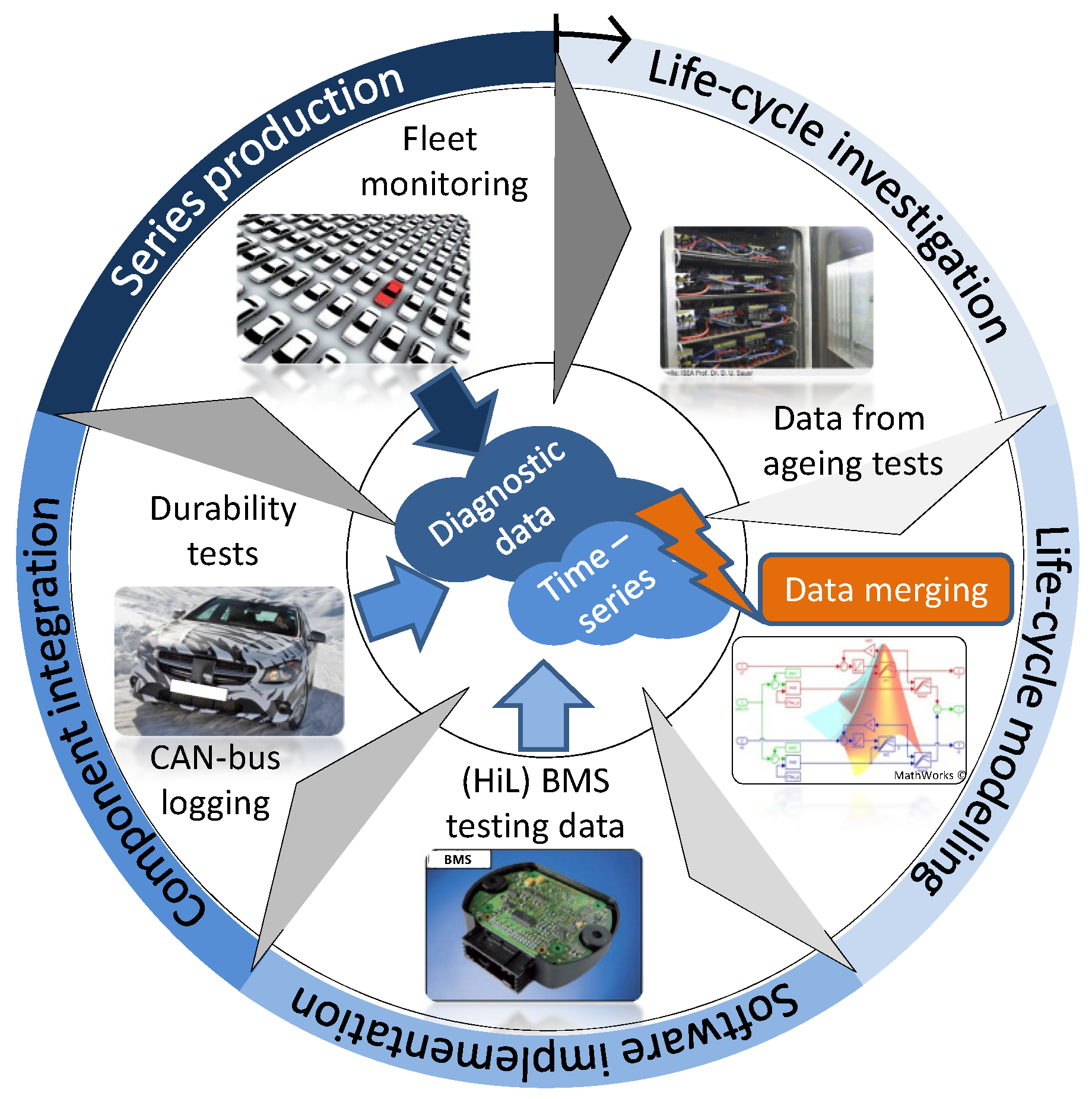
Original equipment manufacturers (OEMs) are concerned with performance losses as well as battery health and life-time restrictions when bringing the lithium-ion battery technology to the customers. Power and capacity fade are two primary metrics of lithium-ion battery degradation impacting directly the customer range and confidence, especially the latter one [1]. However, battery fade is a complex phenomenon provoked by environmental conditions and utilization modes [2]. In an attempt to capture the real-world utilization impacts on battery degradation, OEMs perform, at the first step of an automotive development cycle for lithium-ion batteries as shown in Figure 1, ageing tests on single cells by applying realistic duty cycles on them [3,4]. However, these duty cycles are vague approximations and do not account for the daily variation and unpredictability of such a system [5]. One way to deal with this uncertainty in life-cycle assessment is to oversize the battery and to narrow its operating window to ensure that the vehicle meets minimum requirements like acceleration possibility and available range at the end of its life-time.
This waste of performance and also expenses can be avoided and still a life-time and cost optimized battery can be developed. Real-time monitoring of certain battery internal dynamics unlocks their full potential by enabling an operation near physical limits without sacrificing safety and/or durability. The states and parameters of these internal dynamics are directly measurable only with invasive methods in specialized laboratory environments. Hence, the core challenge for acquiring these internal states and parameters lies in their computation which is based on the only available information in real-time consisting of the measurements of voltage, current and temperature. In the existing literature, the different real-time state and parameter estimation algorithms for lithium-ion batteries can be broadly classified based on the kind of model used: (1) data-driven approaches [6], (2) equivalent circuit model-based algorithms (ECM) [7,8] and (3) electrochemical model-based [9,10,11,12,13,14,15]. The latter ones are derived from electrochemical principles that describe intercalation and diffusion of lithium-ions and the electrochemical kinetics of battery electrodes with the merit of ensuring each model parameter to retain a proper physical meaning. Full order pseudo-two-dimensional (P2D) electrochemical models consist of coupled non-linear partial differential equations (PDE). Such a model was developed in [9] and validated over a wide temperature and current range. Although, this model can accurately predict internal state variables, the difficult mathematical structure of P2D models is generally too complex for suitable estimator/observer design. This circumstance has led to different kinds of model reduction techniques before the estimator is designed. Following this, in [10] a data-driven model-reduction method for a strict electrochemical model was introduced. The gained model is compared to the original electrochemical model from [9], showing a very high approximation quality. A similar approach was done by [11] where a P2D battery model is simulated first to obtain data for the proposed subsystem identification approach. Another way to reduce the order of an electrochemical model is to approximate the electrodes as spherical particles resulting in a single particle model (SPM). This model is very often used in combination with classical observers, such as the Kalman Filter and the Luenberger observer. In addition, there also exist alternative designs for adaptive observers based on a non-linear geometric observer approach for state of charge (SoC) estimation [12] or for simultaneous SoC and SoH estimation including a backstepping PDE state estimator, Padé-based parameter identifier, non-linear identifiability analysis and adaptive output function inversion [13]. Furthermore, to overcome the simplification by only considering electrochemical dynamics under isothermal conditions, the authors in [14] combined a SPM along with lumped thermal dynamics to derive adaptive observers. In a further study, the same authors adopted the electrochemical-thermal model approach together with sliding mode observer methodology to be able to detect, isolate and estimate some battery internal electrochemical faults [15].
Fault diagnosis in lithium-ion batteries has seen a growing interest among industry and academic researchers in the past decade. Model-based fault diagnosis techniques have been extensively applied to the challenge of accurate fault diagnosis in lithium-ion batteries due to their inherent benefits of lower costs and high flexibility. For real-time applications, the aforementioned ECM algorithms have the benefit of their simple formulation and good representation of battery dynamics without high computational power demand. Often used equivalent circuits are extensions to the Thevenin model, with an additional RC parallel circuit [7,8]. The equivalent circuit parameters have to be modelled as functions of different operating conditions such as SoC, temperature and current to capture the battery behaviour over a large operating range, including signature faults. Multiples of these signature faults can be extracted to provide a set of conditions to be detected in case of an upcoming emergency. The authors in [7] define some battery operation like overcharge and overdischarge as possible faults by extracting the desired equivalent circuit parameters via an offline electrochemical impedance spectroscopy (EIS). After obtaining the ECM for the two signature faults, they apply a multi-model adaptive estimation technique for detecting and diagnosing a possible overcharge or overdischarge in the battery operation. Completely new possibilities are opened when the battery operational parameters like the states of internal battery dynamics, estimated by the aforementioned approaches, are available for a fleet management system.
There exist many studies that aim to optimize the battery operational utilization of (hybrid) electrical vehicles (H)EV to reduce costs and identify preventive maintenance activities. An early work which addresses the benefits of a computer-based BMS for recording and subsequent analysis of battery operational parameters can be found in [16]. The authors stated that each user of a fleet has different requirements, and therefore the software-driven BMS should be adapted for particular users to enable an efficient overall management of a current fleet. The keyword to achieve this task is an active fleet management—a personalized health monitoring of every battery built in a hybrid or electric vehicle by telematics devices [17], as the final step in the product development cycle of Figure 1. Such a system is usually set up on a telematics data server containing a large amount of raw data packets collected from the vehicles of a fleet, during diagnostic sessions in dealer’s workshops, or via telematics devices over-the-air [18]. Therefore, this data is filtered and analysed in various aspects, e.g., to identify an imminent failure of a component. At this point, the first of the aforementioned state estimation models, the so-called data-driven approach emerges and provide significant advantages over the electrochemical model-based and the ECM. The often reported main drawback of data-driven approaches, like the requirement of a large amount of data over the whole operating range, is not so significant in an automotive environment. As Figure 1 shows, single components like the cells or the whole product passes through different stages of development resulting in each step in a large amount of well sorted and documented data covering the whole operating range for which the final product is specified. Thus, the data-driven approaches are the first choice for a state estimation model in an automotive environment. One way to deal with such large databases and to calculate the remaining capacity of an entire fleet is already shown in [19]. The authors set up a hypothesis that all the batteries in the fleet will age the same way as investigated battery modules come from the same serial production. In contrast, our approach requires an accurate estimation of degradation parameters of a lithium-ion battery and a prognosis for their future deployment on-board each vehicle.
The aim of this contribution is the development of a novel data-driven battery health monitoring algorithm with a degradation prognosis capability particularly adapted for usage in a fleet management system. The idea behind such a system is to identify a potential failure of each battery build in a vehicle based on that degradation prognosis data, so preventive maintenance activities could be started. Due to limited capability of transfer devices, the received raw data by a telematics server is limited in its amount—it is of diagnostic data type, as shown in Figure 1, with finite information contained. Therefore, an on-board health monitoring algorithm needs to calculate an individual degradation prognosis model for each battery and provides a limited model parameter set via diagnostic devices to the fleet management system. Furthermore, as battery degradation is unique for each vehicle, because of various environmental conditions and application modes, the real-world utilization needs to be captured in compact form and provided in addition to the degradation model parameters.
2. Life-Cycle Investigation on Cell and Battery Level
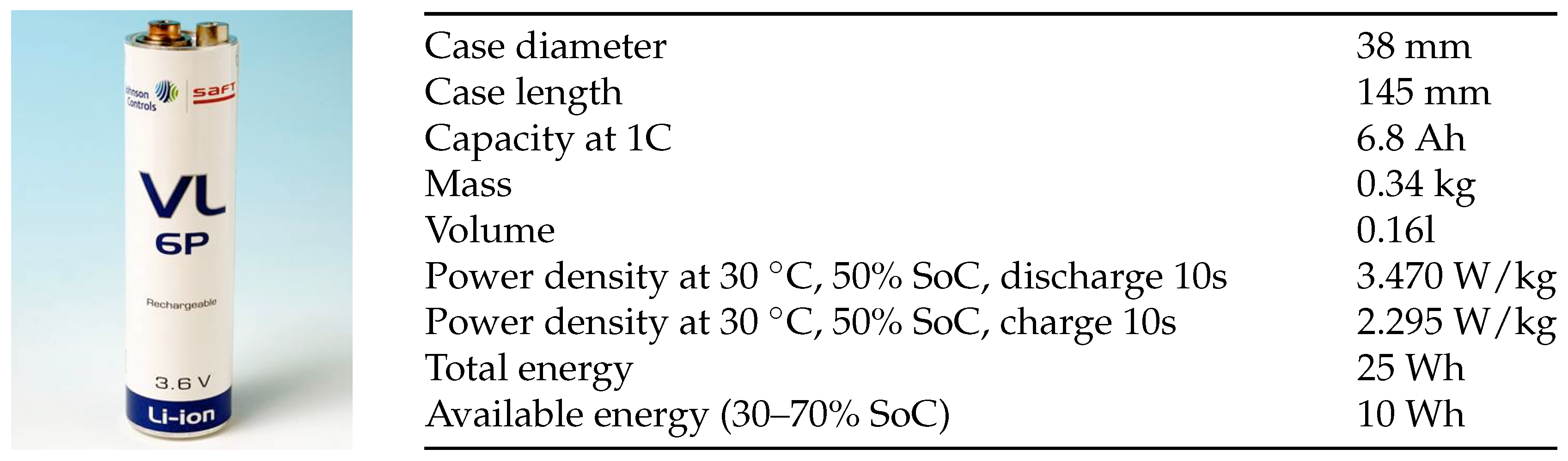
The typical life-cycle investigation on lithium-ion cells usually starts with a large scale of cell degradation tests with a pre-defined duty-cycle. For this work, 12 high-power lithium-ion cells for automotive application in hybrid vehicles were used for the experimental investigation on cell level. The deployed cell is shown in Figure 2 together with its main specification, taken from [20]. The cell has a nickel-cobalt-aluminium (NCA) cathode chemistry and is well known for its excellent calendar and cycle life which was already reported in [21]. The experimental investigation was performed on an automated testing equipment consisting of a climate chamber to simulate the different operating temperatures and a programmable electronic load. To obtain comparable starting conditions for the cycling, every test scenario begins with a full cycle, which implies one full discharge and one full charge with 1 C current. After a relaxation time, which was dependent on the adjusted climate chamber temperature, the cells are discharged to a certain SoC value before the actual cycling starts. The performed testing scenarios on cell and battery level differ in terms of their ambient temperature, the start-SoC and load profile, named in this investigation from HV1 to HV12. They are summarized in Table 1 and Table 2 for each tested cell, numbered from 535–540 and 605–610, as well as for the two tested batteries (nr. 4198 & nr. 2041). At the end of each testing scenario, capacity tests were made, so the cells’ performances could be monitored during the whole testing time. Each charging and discharging during the capacity tests is done with the constant current constant voltage (CCCV) method.
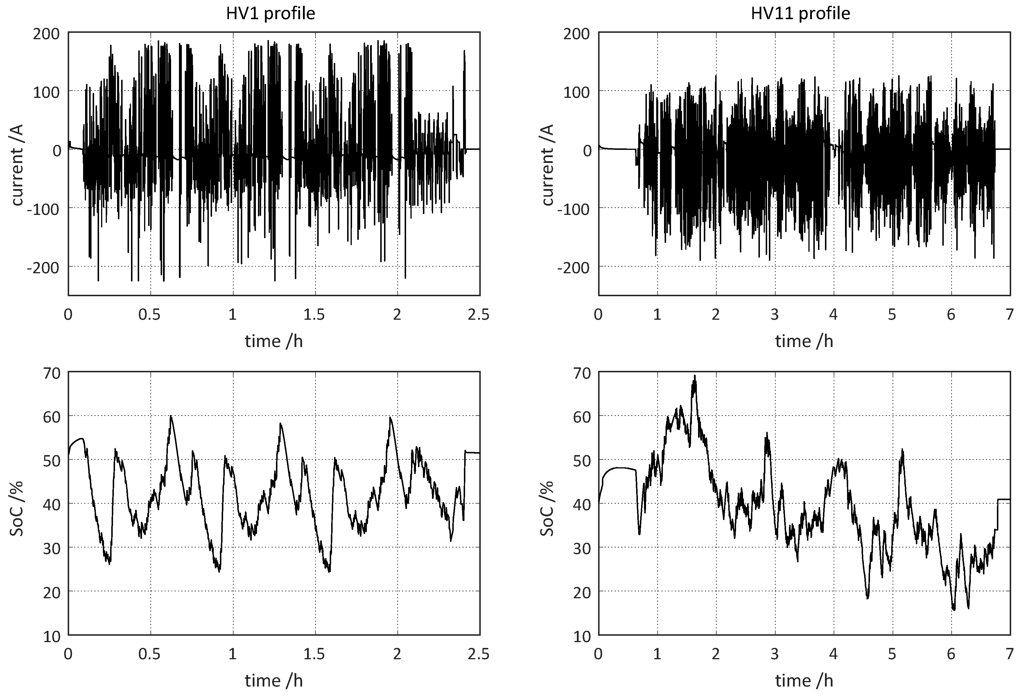
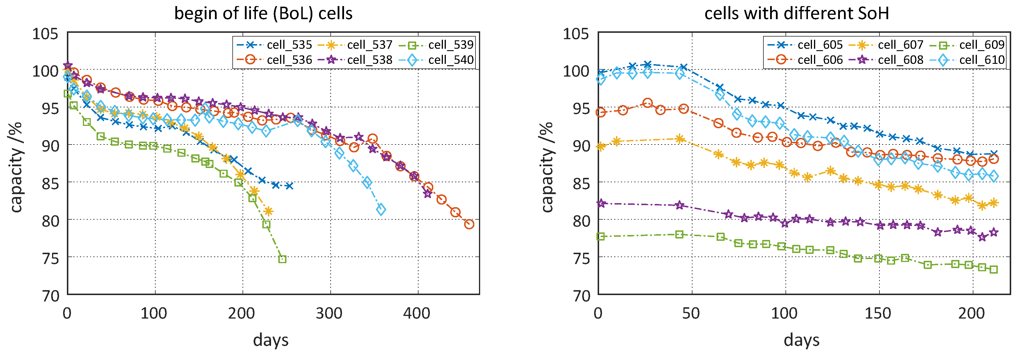
The cells 535–540 experienced a cyclically repeated real-world current profile (HV1) shown on the upper left corner of Figure 3 together with the corresponding SoC-trend on the plot below. The cycling was performed at room temperature, with different start-SoC levels for each pair of three cells. The only modification in the test procedure was switching the start-SoC from 55% to 45% for the cell number 535. If the test scenarios in a certain time period remained unvaried, they are indicated with a ditto mark (″) in the Table 1. The impact of the different start-SoC levels on the degradation behaviour is obvious, when considering the time when the cells reached their end of life (EoL) criteria. While the cells starting with 45% SoC remained in the test over a year, the cells with a start-SoC of 55% reached their EoL already after 250 days. The resulting capacity loss that occurred during cycling can be observed in the left graph of Figure 4.
Due to changes in the start-SoC, the cell 535 shows a slightly different ageing behaviour compared to the two cells which remained at the higher SoC level. The cell shows even recovery symptoms so that the remaining capacity is higher by almost 10% when this pair of three cells reached their EoL defined by 85% of remaining capacity. By considering these results, the following question arises immediately: how can one be assured that the tested duty-cycle HV1 is representative of real-world loads?
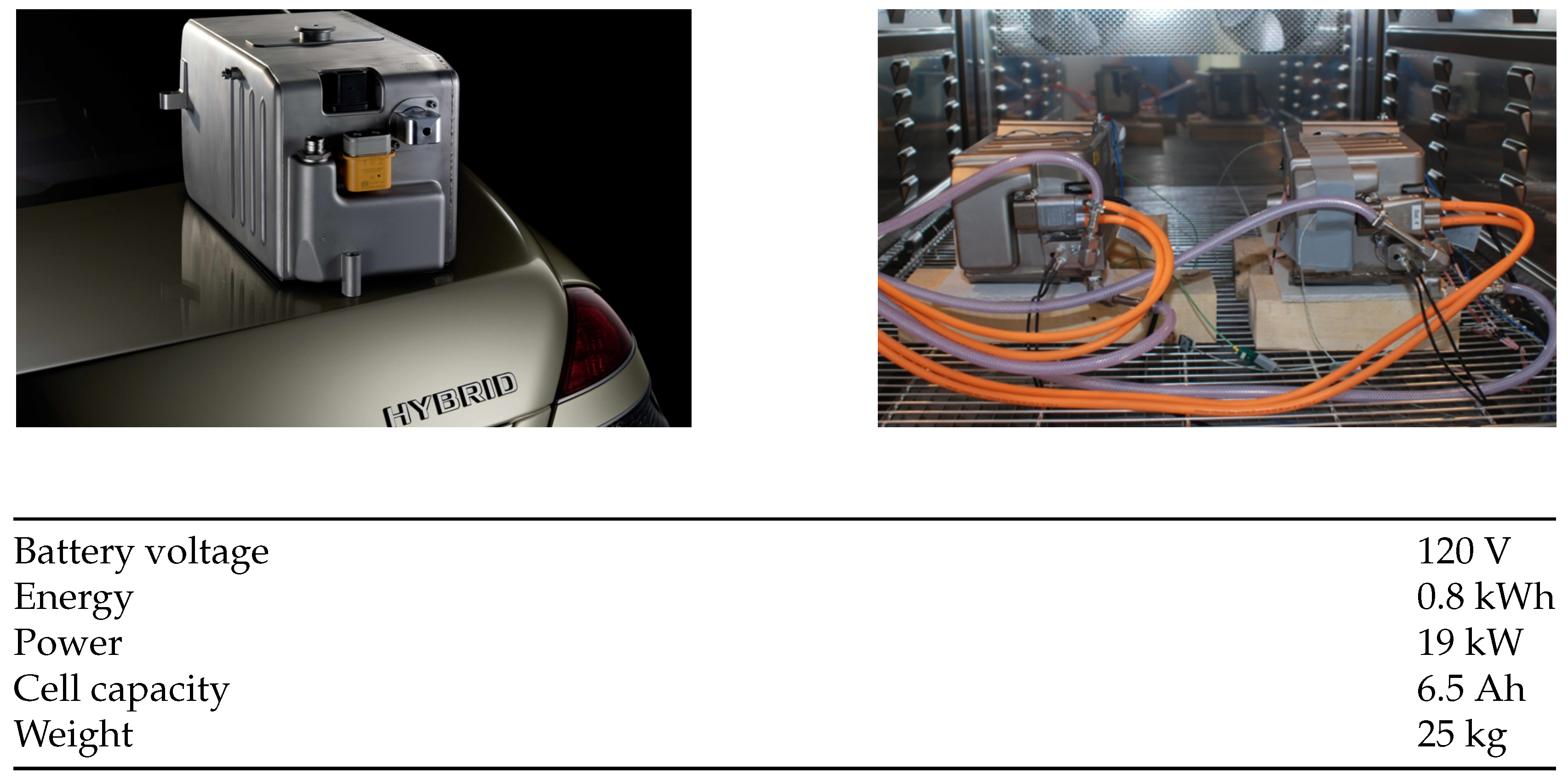
To counteract this unilateral life-cycle investigation result, intensive endurance tests were performed with different Mercedes-Benz hybrid vehicles to capture the various operating conditions with the build-in data-loggers [22]. This vehicle type is equipped with a lithium-ion battery, which is shown in Figure 5, while the main electrical characteristics of this battery are summarized in the table below. One of these recorded load profiles is introduced by the Figure 3, on the upper right corner with the corresponding SoC-trend below, and lasts about 6 h. Such varying real-word load profiles, recorded at different temperature- and SoC-levels, occur at the third and fourth stage of the development cycle in Figure 1. To obtain testing conditions as close as possible to real operation, it is indispensable to use this recorded data for the cyclic ageing of single cells. Therefore, the cells 605–610 were exposed to much more varying load profiles (HV2-HV12), ambient temperatures and start-SoCs as this was the case for the cells from Table 1. The detailed test sequences can be seen from Table 2.
The observed capacity loss is given in the right graph of Figure 4 and shows a more differentiated capacity fade over time for each cell. It can be concluded that some of the load profiles were more intensive and affected capacity fade more heavily, while others were quite mild. Furthermore, the capacity values are scattered already at the begin of the cycle life investigation. Although the cells were taken from the same batch after production, three cells were already exposed to cycle ageing prior to this investigation and the other three cells were stored at room temperature during this time and therefore show higher capacities. In this way, the impact of a certain load profile on different levels of solid electrolyte interphase (SEI) formation in the particular cells should be demonstrated.
Furthermore, the recorded real-world duty cycles (HV6-HV12) were disposed to two lithium-ion batteries in laboratory conditions over a long period of time as shown on the right side of Figure 5. Again, one battery was taken directly after production whereas the second one already experienced a usage during vehicle endurance testing for over 50.000 km. The batteries were operated in an environment identical to their installation space in a vehicle in terms of ambient temperature and battery cooling. The conducted test sequence can be seen in Table 2. For most of the testing time, both batteries underwent the same load profile except one short period where the profile differs for each battery. As it is not possible to cyclically investigate enough batteries in laboratory conditions to represent a whole fleet, single cells of each battery will represent single (H)EVs in the further course of this work. This simplification is legitimated by the individual physical behaviour of each of the 35 single cells inside one battery. Their internal parameters like the resistance, the capacity or the self-discharge rate diverges from cell to cell. In this way, a small “fleet” of seventy “vehicles”, which all slightly differ, is available for validation purposes. The next section will show how the measured time-transient data during cell and battery testing is converted to a data type which is available in a fleet management system.
3. Modelling the Ageing Behaviour of Lithium-Ion Cells
A key step of an automotive development cycle for lithium-ion batteries is the development of an accurate ageing model. Such a model formulates the degradation process as a function of battery operations [23] and is therefore indispensable in the early product development phase. When it is built upon real-world battery operation data, an accurate ageing model performs estimations about degradation behaviour of the utilized lithium-ion cell type, to ensure its life expectancy as a battery component. However, an ageing model—depending on the modelling approach—can also be an important element of the BMS. By being part of a continuous health monitoring process, it observes the vital battery parameters like the actual capacity and performs prognosis for their deployment. Furthermore, such a health monitoring process produces also an output relevant for a fleet management system when accessible e.g., during dealer’s workshops, or via telematics devices over-the-air. This is only possible if the process output data is of diagnostic type.
The decision to implement an ageing model into a BMS for degradation prognosis purposes depends, beside the chosen modelling approach, mostly on the accuracy of such a model. By being modelled only on life-cycle investigation data, it is hardly to believe that such a model will perform well in all possible operation conditions over lifetime. Therefore, all real-world battery operation data which come up during the software implementation and testing phase of the BMS as well as data from durability tests with whole batteries, should be considered in the modelling of the ageing behaviour. The basics for this approach are introduced in the next subsections.
3.1. Data Preprocessing by Histograms—Load Collectives
By considering the different data types generated during the whole battery development cycle from Figure 1, the following question arises: how can the relevant information for the modelling of the ageing behaviour contained in the data be merged together? Time-transient data from laboratory investigations on cells and from CAN-bus data-loggers in (H)EVs need a uniform consideration as well as the diagnostic data received by a fleet management system. An appropriate way to achieve this is to convert time-transient battery operation data into histograms by following clearly defined rules. As this idea is not new, it was already published in [6,24]; the present work introduces a further modification of it.
Building histograms of time-transient data results in a massive data reduction and, therefore, loss of relevant information. The idea behind using histograms is to put the information contained in the resulting distributions in relationship with the observed capacity fade. The capacity is a relatively slow changing internal battery parameter, calculated e.g., by coulomb-counting and only at certain battery operation events like the charging procedure. This results in relatively long lasting time series in the interval between two proper calculated capacity values that need to be transformed into histograms. These time series can contain several billions of data-points, so the classical rules for defining the number of histogram bins would fail resulting in thousands of bins as these rules are dependent on the data length. The interesting histogram central moments like mean, variance and standard deviation can be calculated by a moving window approach directly on times-series data. However, this reduces the large amount of data-points only to three relevant values which is too much data reduction. Therefore, a time series of battery relevant signals like the current, cell-voltages, temperature or SoC measured in a time interval between two calculated capacity values needs to be separated into segments first before converting them into histograms – or so called load collectives in our case.
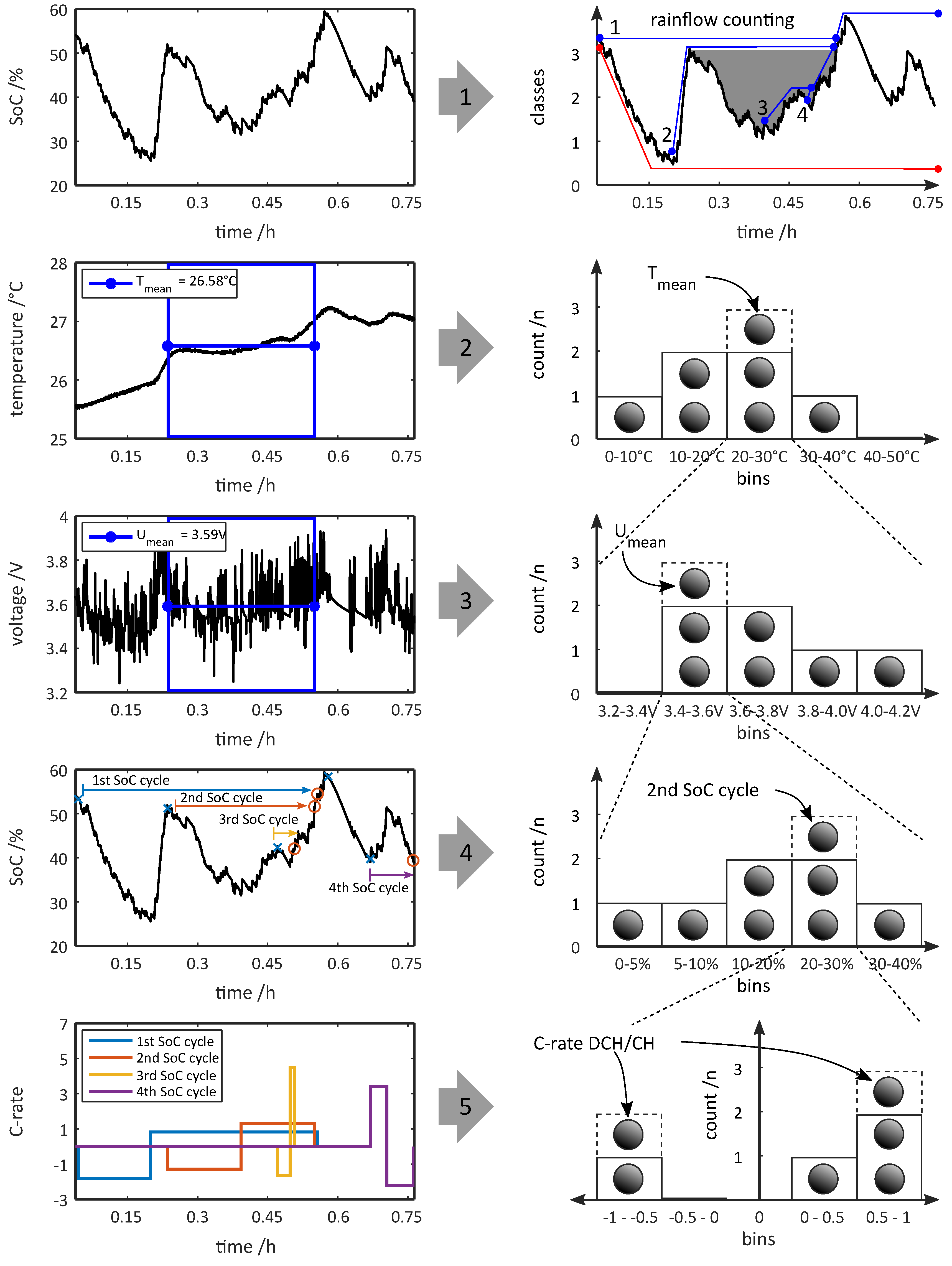
Although there exist some really interesting Bayesian approaches for finding change points in time series for their segmentation [25], we prefer a more “controllable” approach with the well known rainflow-counting algorithm from machinery. In [6], an application of this algorithm for counting the depth of discharges (DoD) in the SoC-signal was shown, in which the resulting cycles were classified in their mean and amplitude afterwards. Later on, an improvement to this cycle counting was introduced in [24] by explaining each DoD-cycle in a time series by its corresponding charge and discharge-rate. Furthermore, each DoD-cycle has its corresponding mean cell voltage and temperature which can also be classified by a histogram. At this point, we introduce our new approach to build the histograms from battery data, the so-called “nested” load collective, for which the construction procedure is shown in Figure 6.
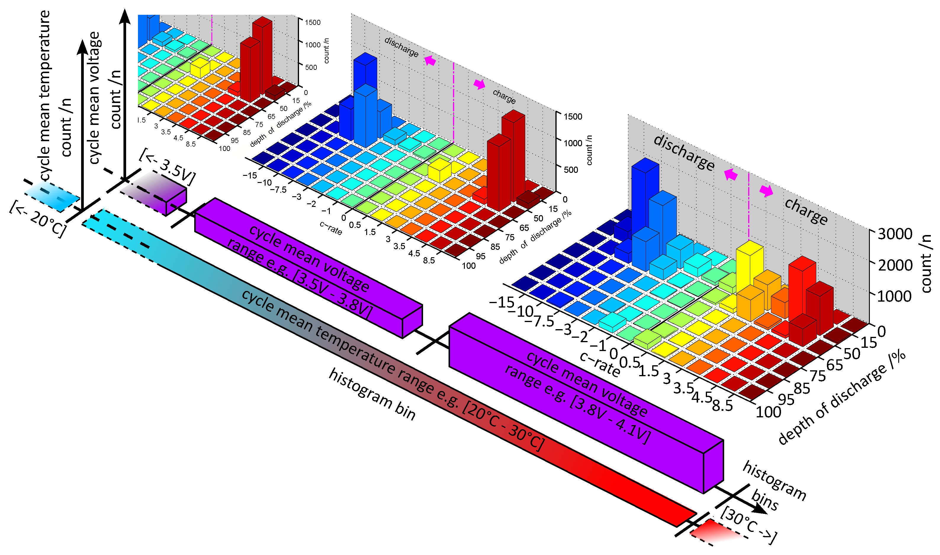
By following the numeration in Figure 6, the rainflow algorithm identifies the existent SoC-cycles first, in the shown section of the HV1 profile from Figure 3. A good way to describe the rainflow algorithm is to imagine rain drops falling down a pagoda-style roof. The rain-drops arise at the maximum of the curve, flow to the next minimum and drop down, e.g., the red line. Or they arise at a minimum and flow to the next maximum of the curve (if the diagram is rotated by 90° clockwise) to drop down. Rainflows starting from a lower minimum interrupt, the rainflows which start at a higher one, e.g., the blue line starting from 3 is interrupted by the blue line starting at 2. In this way, four SoC-cycles are identified in the shown profile section. For the time-period of each of these cycles, the mean temperature and voltage is calculated in the next two steps, shown in the 2nd and 3rd graph on the left side of Figure 6. The last step of the proposed procedure provides a calculation of an approximated C-rate according to [24] for each SoC-cycle shown in the fourth graph. The histogram building procedure on the right side of Figure 6 can be demonstrated e.g., for the time-period of the SoC-cycle which is highlighted in grey in the upper right plot of Figure 6. After classifying the mean temperature of the same time-period in a 1D-histogram in the second step of the procedure, the mean voltage in the identical time-period (blue rectangles in the second and third graphs on the left) is calculated and stored in a further 1D-histogram, but which is “nested” into the “20–30 °C” bin of the temperature histogram. As the fourth step of the procedure, the grey highlighted 2nd SoC-cycle is stored into the corresponding 1D-histogram, connected to the “3.4 V–3.6 V” bin of the voltage histogram. As the final step, for the 2nd SoC-cycle, an approximated C-rate is calculated and stored separately for the discharge and charge rate in the last 1D-histogram, again “nested” into the certain bin of the histogram from one step before. This procedure results in a complex load collective which is shown as an exemplary illustration in Figure 7. By nesting the load collectives, interaction effects can be considered. Therefore, our expectation of this procedure is to preserve as much relevant information from the time series data as possible for our model-based approach.
3.2. Data-Driven Modelling
In Section 1, different real-time state and parameter estimation algorithms from literature, based either on electrochemical or equivalent circuit models, were presented. However, for this approach it is often difficult to determine the model parameters [26]. The strength of a data-driven modelling technique is the ability to transform high-dimensional and noisy data into lower dimensional information for diagnostic or prognostics tasks. The main drawback of such approaches is that their efficiency is highly dependent on the quantity and quality of operational data from the system which needs to be modelled [27]. As this work commences with an experimental investigation on a large scale in Section 2, the amount of available data will suffice for an in-depth validation of our already proposed data-driven model from [6]. In addition, the present work introduces an alternative probabilistic modelling approach, which is used for comparison purposes. These two modelling techniques are now introduced in the following subsections.
3.2.1. Support Vector Regression
Support vector regression (SVR) has been used in connection with load collectives as the basic data to health monitoring purposes of lithium-ion batteries, e.g., in [6]. A detailed tutorial on this method can be found in [28], on which this paragraph is based. Given training data , the goal of support vector regression is to find a function which has at most deviation from the values and is as flat as possible. First, assume is linear, hence it has the form . To ensure flatness, one has to minimize . In addition, constraints have to make sure that the deviation between and is not larger than . However, this is often not feasible. Hence, one has to allow for errors and introduce slack variables, here denoted by and . This results in the following optimization problem [28]:
The constant C describes the trade-off between the flatness of and the errors. In many cases, the optimization problem in (1) can be solved more easily in its dual formulation [28]. The solution of this problem is
where and stand for the Lagrange multipliers from the Lagrange function of the optimization problem. If either or is non-zero, is called a support vector.
So far, was assumed to be linear. The algorithm can be extended to the non-linear case by mapping into some feature space using a non-linear map and by applying support vector regression afterwards. Unfortunately, this might be computationally infeasible. However, (2) shows that only depends on the dot product of and x. Hence, one only needs to know the dot product between the mappings of and x, not the mapping itself. This dot product, , corresponds to a kernel function . Hence, can be expressed as
The kernel function has to satisfy certain conditions, which can be found in [28].
3.2.2. Relevance Vector Machine for Regression
Relevance vector machines (RVM) have been used for forecasts related to lithium-ion batteries, for instance in [26,29]. This introduction follows them as well as [30]. In this work, a RVM is adopted for use with load collective data for the first time. Suppose we are given measurements adopted to use with histograms from the dependent variable and from inputs . Their relationship is described by a model and error . This can be expressed by [30]
The errors are assumed to be independent, normally distributed random variables with mean zero and variance . Hence, the joint probability density function of the errors is given by
The model is a linear combination of basis functions [30]. Hence, , w being a vector of weights and . In matrix notation, equation (4) can be written as
where is a matrix containing . The aim is to find values for w such that generalises well to new data and w is sparse, which means that most elements of w are equal to zero. Sparsity controls the complexity of the model and avoids overfitting. Furthermore, it is useful if memory resources are limited as in the case of a battery management system. The training vectors , which are associated with non-zero elements of w, are called relevance vectors. Using the normality assumption in (5), one can derive the likelihood function [30]
One approach might be to maximize the likelihood with respect to w. However, this can result in overfitting because the complexity of the model is not controlled [30]. Controlling complexity means to control the growth of the weights in w. In a bayesian setting, this is done by using a prior distribution on w [30]. It is specified by . stand for hyperparameters which have their own prior distribution given by , where a and b stand for the parameters of the gamma distribution. In addition, there is a prior distribution for the inverse variance . In accordance with the literature, we set . Its prior distribution is specified as , where c and d are the parameters of the gamma distribution. Using the likelihood, the prior distributions and Bayes’ theorem, one can calculate , as it is done in [29]. This distribution can be used to compute the predictive distribution as in [30]. It is given by
3.3. Incremental Approach for On-Board Implementation
Batch versions of SVR and RVM, which are introduced in the two subsections above, have to be retrained from scratch whenever a new data point is added to the training set. This is not feasible for on-board applications, because the whole data set used for batch training would have to be stored on board. Hence, an incremental approach is used. This incremental approach is based on the idea of [31] for support vector machines, which was extended to relevance vector machines in [26]. The procedure is the following: whenever a new data point comes in and the last prediction error was higher than a certain threshold, a new training set is created consisting of the relevance vectors and the new data point. The relevance vector machine is subsequently retrained using the new training set. With this approach, the data points from the former training set which were no relevance vectors are deleted. This leads to low memory requirements, because only the relevance vectors and the new data point have to be stored. However, one should be aware that potential future relevance vectors are also deleted. The procedure for support vector regression is similar, with the only difference being that support vectors are used instead of relevance vectors.
3.4. Parameter Tuning and Feature Selection
For support vector regression, the hyper-parameters C, and a kernel parameter (in our case for a Gaussian kernel) have to be chosen. For the relevance vector machine, a parameter of the basis function has to be selected. Furthermore, a feature selection has to be conducted, too. Both tasks are done using repeated grid-search cross-validation for variable selection and parameter tuning as described in [32]. The feature selection method used in the repeated grid-search cross-validation is the regressional relief-F algorithm (RRELIEFF) from [33]. The selection of hyper-parameters and variables takes place in the batch case. They are not changed during incremental learning because of the computational restrictions of the battery management system.
3.5. Degradation Prognosis Approach
A simple degradation prognosis approach feasible for on-board implementation was already introduced in [6]. As the future battery operation is not known, one option is to multiply the already stored values in the load collectives by a factor to achieve a battery load extrapolation. This extrapolated load collectives serve as the input for an incremental SVM or RVM implemented on-board, to estimate the capacity value in the near feature. Due to limited computational capabilities on-board, more sophisticated approaches in modelling load variability especially for machinery [34] are reserved only for off-board use.
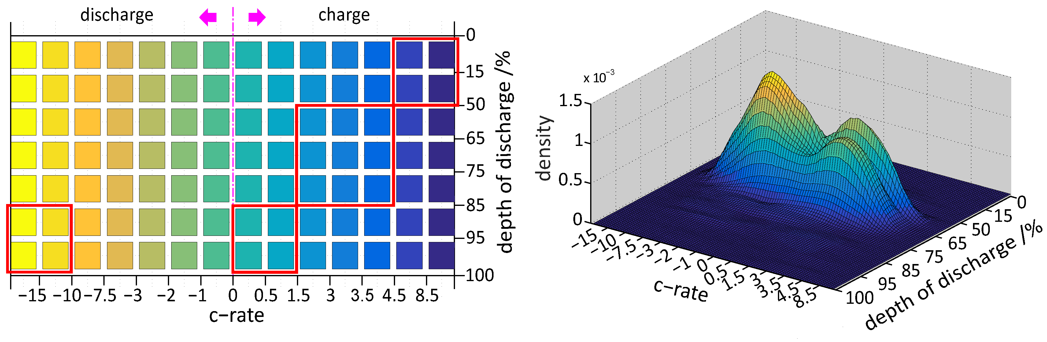
At this point, we introduce a utilization of these methods to extrapolate the described load collectives of a battery for the first time reported in literature. By examining the 2D-histogram from Figure 7, it is evident that this discrete distribution has many empty bins in some regions. It is expected that many of these bins would have counts in them if the battery would operate for a longer time. An expected, load collective for any desired number of counted DoD-cycles from Figure 7 could be constructed by randomly placing cycles into the histogram. Each cycle is placed then into the histogram with the choice of bins weighted by the probability of each bin so that the bins with higher probabilities have more cycles on average. The probability of each bin is estimated and smoothed using a kernel density estimator on the data set of the histogram [34]. This data set consists of the mean of each bin appearing according to the number of data points in the respective bin.
The kernel density estimator for a sample for is defined as [35]
where K denotes the kernel function. As in [34], the Epanechnikov kernel function was chosen. An example for extrapolating the SoC/C-rate 2D-histogram from Figure 7 at 20–30 °C and 3.4–3.6 V for the HV1-profile with this kernel type, is shown on the right side of Figure 8 below.
Furthermore, the variability in histograms can be modelled individually by defining “damage” regions in the load collective directly as shown with red rectangles in Figure 8 on the left. These regions can also have a physical background; it is well-known that high loading currents at low temperatures can have an influence on the ageing due to lithium plating [21] or a high discharging current affects ageing, too. By choosing different bandwidths for the kernel in certain regions of the load collective, more variability can be achieved in them resulting in a histogram extrapolation that affects the ageing most.
4. Model Implementation and Usage by Fleet Management System
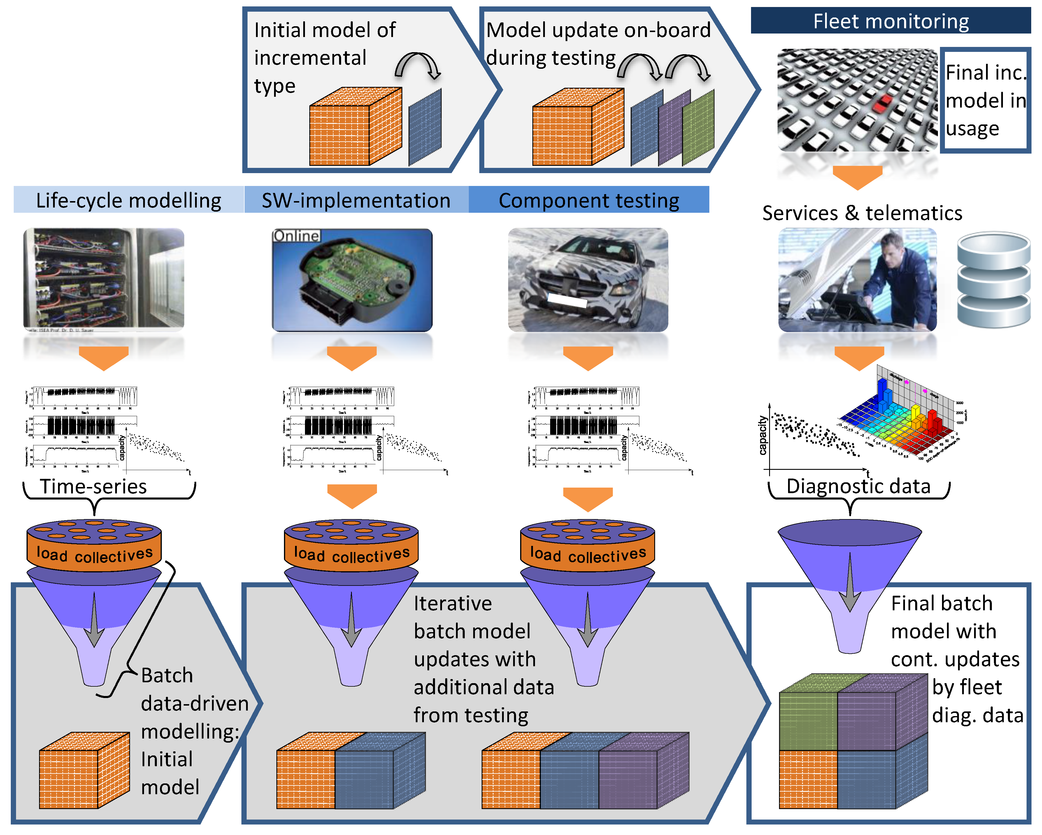
Finally, after explaining the basics for our battery degradation modelling and prognosis approach, the model implementation and usage by a fleet management system is introduced in Figure 9. We distinguish between a model implementation on-board the BMS (arrows at the top) and a model for off-board usage (bottom arrows), on workstations with installed MATLAB© software. The single steps from the battery development cycle of Figure 1 are shown vertically from the left to the right of the picture. The initial degradation model is firstly built by a batch-modelling process based on experimental data from life-cycle investigations on single cells, as introduced in Figure 4. The conversion of time series data from the laboratory is performed by load collectives to obtain the desired distributions of all battery relevant signals according to Section 3.1. This is performed every time new data is available in the following product development steps, e.g., during BMS testing or endurance tests of vehicles. Thus, it is obvious why the circumstance with building load collectives is indispensable. If diagnostic data from a certain fleet, which is accessible via diagnostic sessions in dealers’ workshops or via telematic devices i.e., according to [18], the data contains load collectives with an identical structure as they were used in the batch-modelling process from the beginning; the developed degradation model can actively support the fleet management in health monitoring and prognosis.
Furthermore, the initial batch model is iteratively updated by incoming data during further battery development steps and in this way gathers additional “knowledge” about the different degradation behaviours from varying operating conditions, e.g., during endurance tests in hot or cold countries. At the end, when the series production starts, a final batch model is set up which is able to perform degradation prognosis by our approach from Section 3.5 for each vehicle based on its set of load collectives or even a whole fleet by e.g., averaging their load collectives. Nevertheless, the batch-model updates do not stop here. As part of an active fleet management, the batch-model is updated iteratively by incoming load collectives which may contain further relevant information on battery degradation. The goal behind this procedure is to identify the ageing impacting factors continuously by performing an intensive feature selection on the whole data set, reaching from the life-cycle investigation to the actual point in time. This information is very precious in the planning of life-cycle tests on cells for the next battery product generation.
In parallel to the batch-model, an incremental variant of the initial model can be implemented into the BMS during the software implementation phase together with the new “nested” load collectives. This type of model updates itself incrementally each time a new capacity value is calculated on-board, which happens often during the development phase e.g., by testing vehicles on the roller test bench. After that, an already updated incremental model is ready for series production where further adaptation to the individual degradation of a certain battery takes place. As described in Section 3.5, this model performs a simple degradation prognosis for the capacity value on-board the vehicle which is a valuable input for e.g., variable battery operation window.
5. Results and Discussion
In the past, a lot of battery health monitoring approaches suffered from the unavailability of applicable data for validation. Most of the accomplished investigations are based on very uniform tests, batteries are cycled only at one or a few values of SoC, temperature, and/or DoDs, so that the obtained approaches are at least not validated for an application in real-world dynamical situations. As already introduced, for our approach there exists a portfolio of measurements reaching from life-cycle investigations on lithium-ion cells in laboratory conditions to measurements from endurance tests on battery level which should guarantee a thorough validation of the developed models.
5.1. Batch Model
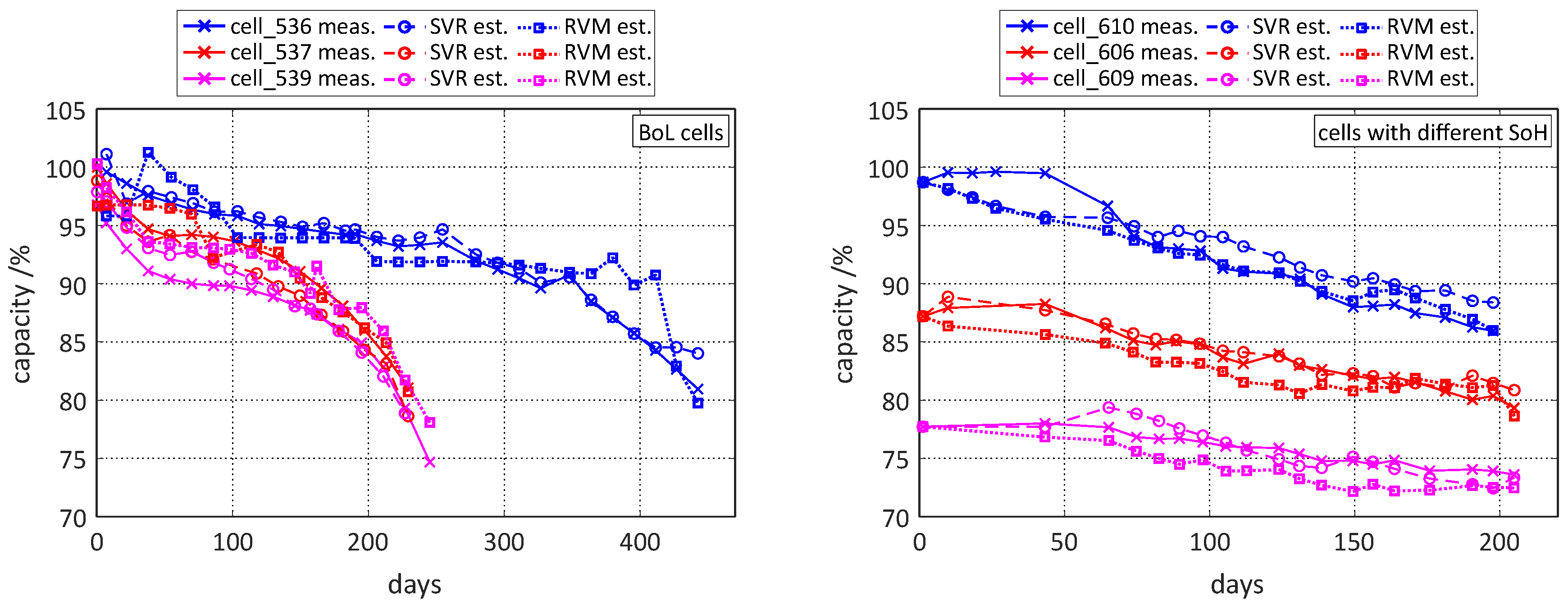
The aim of the batch modelling process in the case of a SVR approach is to find a function which is simultaneously as flat as possible and which approximates the capacity degradation trend the best. By following the steps from Section 3 and starting with a data set of all available input-output pairs of a process, e.g., the ageing behaviour of cells in a life cycle investigation, this process results in the generation of an initial model from Figure 9, which contains only the support vectors. Additionally, the RVM approach also results in establishing an initial model by considering only the life cycle investigation data. This model contains the relevance vectors needed for the predictive distribution function from Equation (8). Figure 10 shows the results of adopting both approaches only on life cycle data (left graph) and on the same data set, but iteratively updated by measurements from vehicle durability testing on the right.
5.2. Incremental Model
This work also introduces an incremental type of the data-driven modelling approaches from Section 3.2. The initial batch models of SVR and RVM type from Figure 9 are both capable for an on-board implementation to the BMS which was already shown in [6].
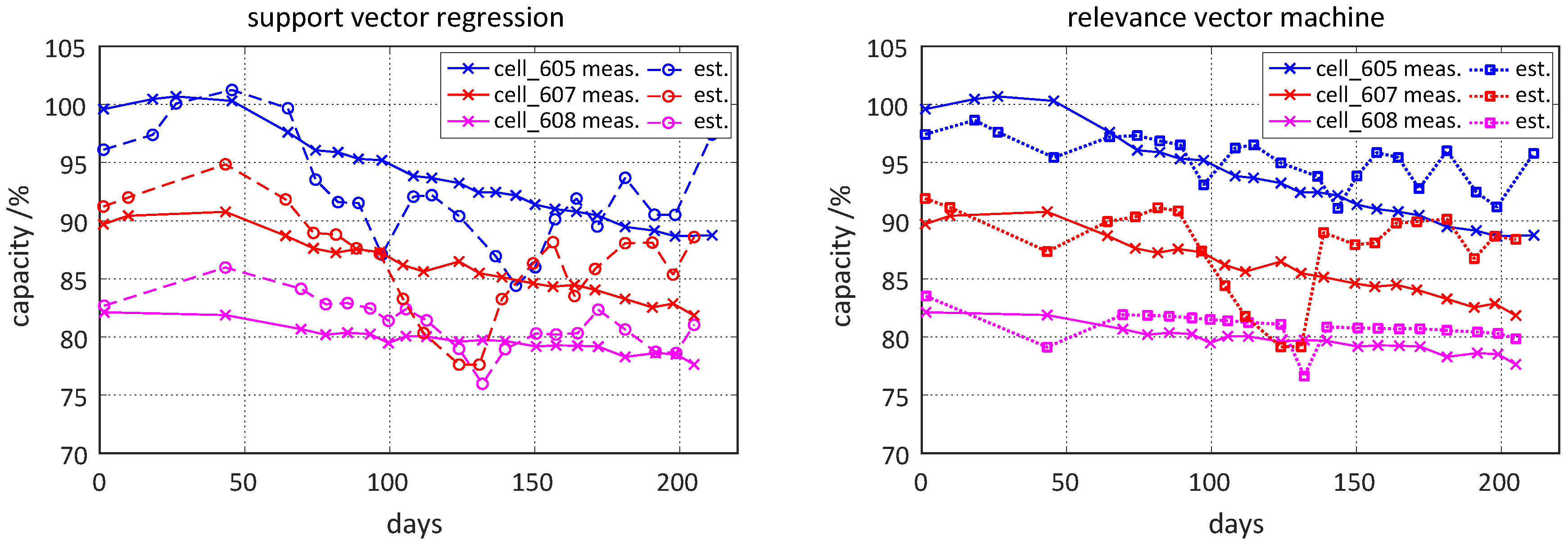
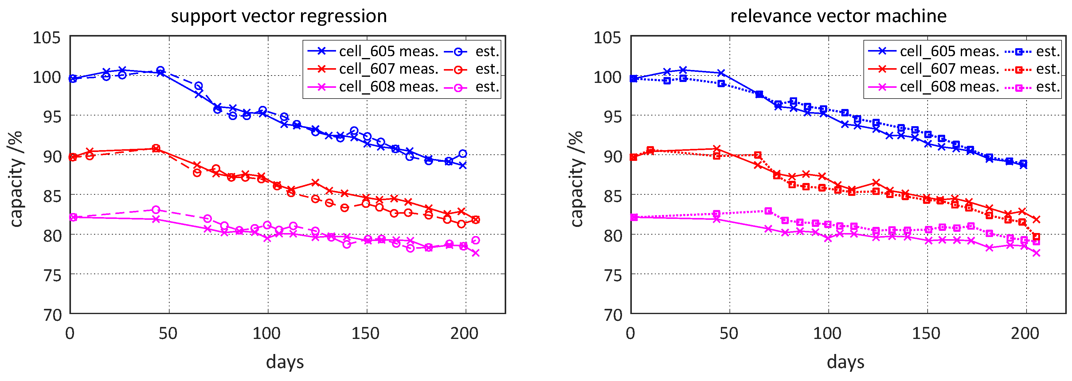
If these initial batch models are only based on data from life cycle investigations without an on-board incremental update enhancement, the prognosis of the capacity degradation is not satisfactory when applied to data from vehicle durability tests as the Figure 11 presents. The reason for that could be a vague duty cycle used in the laboratory investigations which does not represent very well the variability of a real-world battery utilization. Therefore, the support or relevance-vectors of the batch model, stored in the BMS, need an incremental update by new incoming input-output data pairs comprising always a set of load collectives as input and an actual capacity value as the output of a data point. In doing so, an on-board incrementally updated batch model, either of SVR or RVM type, is able to track the capacity degradation trend very precisely as Figure 12 illustrates. In this way, updated data-driven models are in the best position to perform an accurate prognosis of the capacity degradation at every point in time as they incorporate the “knowledge” about the degradation behaviour from the life-cycle investigations on.
By considering the model results from Figure 12, it is obvious that both approaches, either the SVR or the RVM, perform well in terms of tracking the capacity degradation trend when finding new appropriate support or relevance vectors for the incremental model.
However, the RVM has one crucial advantage over the SVR—its model output also provides a probability distribution for the predicted capacity values. This confidence interval contains with 95% probability the true capacity value. Therefore, for further validation, this model type is taken into close consideration.
5.3. On-Board and Fleet Management Prognosis Results
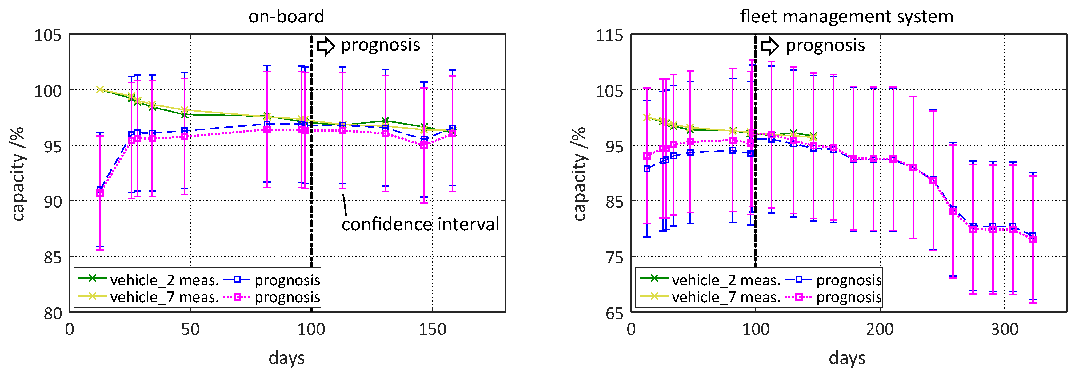
Finally, the prognosis capability of the on-board approach as well as of the fleet management system can be validated on battery data from durability tests of Figure 5. Until now, this data is unseen by the two model approaches, neither by the final RVM batch model from Figure 9 nor the incremental RVM model type, and therefore, represents a future real use case together with the series production start. For clarity, only two cells from a batch of 70 cells were chosen randomly for validation purposes. The prognosis results for the incremental model type are depicted on the left of the Figure 13.
By starting with a quite wrong estimated capacity for both “vehicles”, it can be noticed that the incremental model adapts itself to the degradation trend more and more by hitting it after 100 days of battery utilization. At this point, a first capacity prognosis for the next slightly more than 50 days can be started by generating input data for the incremental RVM through repeating the very last available set of load collectives from the BMS memory multiple times. This results for both “vehicles” in a predicted capacity degradation, which is pretty close to the measured capacity trend. It is remarkable that, straight after the second incremental update, all the measured capacity values lie inside the confidence interval which should in fact contain the true capacity value with a 95% probability.
The prognosis results of the fleet management system are presented on the right of Figure 13. For the first 100 days, the incremental model update is performed on-board and this model, together with all load collectives of this period, are available for the fleet management system according to Figure 9. Now, the received load collectives can be extrapolated by adopting the kernel method from Section 3.5. For that, the load collective counts present on the 100th day can be treated as a whole during extrapolation, resulting in a 100-day long prognosis window whereas a higher resolution for the capacity degradation trend would be preferred. Therefore, the load collective counts are divided into smaller “slices” for extrapolation, resulting in the shown trend of Figure 13. Although the cycling was stopped at 150 days, the prognosis interval was extended up to 300 days to demonstrate the impact of the chosen Epanechnikov kernel. The predicted fast capacity degradation is probably realistic if the cycling has continued and by considering the capacity decay in Figure 4. The rather wide confidence intervals should be investigated more in detail in future work.
6. Conclusions
A novel data-driven battery health monitoring algorithm for usage in fleet management systems was developed. It allows the regression function to adapt to the individual ageing behaviour of the battery. This leads to accurate predictions for the two investigated approaches, the support vector regression and the relevance vector regression. By providing a probability distribution for the predicted vaules, the relevance vector regression has an advantage over the support vector regression as the confidence intervals can be obtained to consider the prediction uncertainty. Since only the respective support relevance vectors have to be stored and not the full training data set, the algorithm has low memory requirements. Another advantage of the algorithm is the possibility of long-term predictions by using extrapolated load collectives by kernel density estimation. In the data under consideration this led to realistic predictions.
Author Contributions
Conceptualization, A.N.; Methodology, A.N. and J.B.; Software, A.N. and J.B.; Validation, A.N. and J.B.; Formal Analysis, J.B.; Investigation, A.N. and J.B.; Resources, A.N.; Data Curation, A.N.; Writing—Original Draft Preparation, A.N.; Writing—Review & Editing, B.S., M.B. and K.D.; Visualization, A.N.; Supervision, B.S., M.B. and K.D.; Project Administration, A.N.
Funding
This research received no external funding.
Conflicts of Interest
The authors declare no conflict of interest.
Abbreviations
The following abbreviations are used in this manuscript:
| SoH | state of health |
| OEM | original equipment manufacturer |
| ECM | equivalent circuit model |
| P2D | pseudo-two-dimensional |
| PDE | partial differential equation |
| SPM | single particle model |
| SoC | state of charge |
| BMS | battery management system |
| EIS | electrochemical impedance spectroscopy |
| (H)EV | (hybrid) electric vehicle |
| NCA | nickel-cobalt-aluminium |
| CCCV | constant current constant voltage |
| EoL | end of life |
| SEI | solid electrolyte interphase |
| CAN | controller area network |
| HiL | hardware in the loop |
| DoD | depth of discharge |
| SVR | support vector regression |
| RVM | relevance vector machines |
| RRELIEFF | regressional relief-F |
References
- Badey, Q.; Cherouvrier, G.; Reynier, Y.; Duffault, J.M.; Franger, S. Ageing forecast of lithium-ion batteries for electric and hybrid vehicles. Curr. Top Electrochem. 2011, 1, 65–79. [Google Scholar]
- Samadani, E.; Mastali, M.; Farhad, S.; Fraser, R.A.; Fowler, M. Li-ion battery performance and degradation in electric vehicles under different usage scenarios. Int. J. Energy Res. 2015, 40, 379–392. [Google Scholar] [CrossRef]
- Danzer, M.A.; Liebau, V.; Maglia, F. Aging of lithium-ion batteries for electric vehicles. In Advances in Battery Technologies for Electric Vehicles; Scrosati, B., Garche, J., Tillmetz, W., Eds.; Woodhead Publishing: Sawston, UK, 2015; pp. 359–387. ISBN 978-1-78242-377-5. [Google Scholar]
- Dubarry, M.; Svoboda, V.; Hwu, R.; Liaw, B.Y. A roadmap to understand battery performance in electric and hybrid vehicle operation. J. Power Source 2007, 174, 366–372. [Google Scholar] [CrossRef]
- Mallia, E.; Finley, D.; Bauman, J.; Goody, M. Using EV Telematics to Monitor Real-World Battery Health for EV Owners and Fleet Operators. In Proceedings of the Electric Vehicle Symposium & Exhibition 29, Montreal, QC, Canada, 19–22 June 2016. [Google Scholar]
- Nuhic, A.; Terzimehic, T.; Soczka-Guth, T.; Buchholz, M.; Dietmayer, K. Health Diagnosis and Remaining Useful Life Prognostics of Lithium-Ion Batteries Using Data-Driven Methods. J. Power Source 2013, 239, 680–688. [Google Scholar] [CrossRef]
- Sidhu, A.; Izadian, A.; Anwar, S. Adaptive Nonlinear Model-Based Fault Diagnosis of Li-Ion Batteries. IEEE Trans. Ind. Electron. 2015, 62, 1002–1011. [Google Scholar] [CrossRef] [Green Version]
- Remmlinger, J.; Buchholz, M.; Meiler, M.; Bernreuter, P.; Dietmayer, K. State-of-health monitoring of lithium-ion batteries in electric vehicles by on-board internal resistance estimation. J. Power Source 2011, 196, 5357–5363. [Google Scholar] [CrossRef]
- Tippmann, S.; Walper, D.; Balboa, L.; Spier, B.; Bessler, W.G. Low-temperature charging of lithium-ion cells part I: Electrochemical modeling and experimental investigation of degradation behavior. J. Power Source 2014, 252, 305–316. [Google Scholar] [CrossRef]
- Remmlinger, J.; Tippmann, S.; Buchholz, M.; Dietmayer, K. Low-temperature charging of lithium-ion cells Part II: Model reduction and application. J. Power Source 2014, 254, 268–276. [Google Scholar] [CrossRef]
- Zhou, X.; Ersal, T.; Stein, J.L.; Bernstein, D.S. Battery Health Diagnostics Using Retrospective-Cost Subsystem Identification: Sensitivity to Noise and Initialization Errors; ASME Paper; ASME: New York, NY, USA, 2013. [Google Scholar] [CrossRef]
- Wang, Y.; Fang, H.; Sahinoglu, Z.; Wada, T.; Hara, S. Adaptive Estimation of the State of Charge for Lithium-Ion Batteries: Nonlinear Geometric Observer Approach. IEEE Trans. Control Syst. Technol. 2015, 23, 948–962. [Google Scholar] [CrossRef] [Green Version]
- Moura, S.J.; Chaturvedi, N.A.; Krstic, M. Adaptive PDE Observer for Battery SOC/SOH Estimation via an Electrochemical Model. ASME J. Dyn. Syst. Meas. Control 2013, 136, 101–110. [Google Scholar] [CrossRef]
- Dey, S.; Ayalew, B.; Pisu, P. Nonlinear Adaptive Observer Design for a Li-Ion Cell Based on Coupled Electrochemical-Thermal Model. ASME J. Dyn. Syst. Meas. Control 2015, 137, 1–12. [Google Scholar] [CrossRef]
- Dey, S.; Ayalew, B. A Diagnostic Scheme for Detection, Isolation and Estimation of Electrochemical Faults in Lithium-Ion Cells. In Proceedings of the ASME 2015 Dynamic Systems and Control Conference, Columbus, OH, USA, 28–30 October 2015; Volume 4. [Google Scholar]
- Lenain, P.; Kechmire, M.; Smaha, J. Monitoring fleets of electric vehicles: optimizing operational use and maintenance. J. Power Source 1994, 53, 335–338. [Google Scholar] [CrossRef]
- Barré, A.; Suard, F.; Gérard, M.; Riu, D. Battery Capacity Estimation and Health Management of an Electric Vehicle Fleet. In Proceedings of the IEEE Vehicle Power and Propulsion (VPCC), Coimbra, Portugal, 27–30 October 2014. [Google Scholar]
- Hermansson, F.; Axelsson, L.; Granström, R. Experiences from Data Collection in Living Labs-The Swedish National Database for Car Movements. In Proceedings of the Electric Vehicle Symposium & Exhibition 29, Montreal, QC, Canada, 19–22 June 2016. [Google Scholar]
- Vichard, L.; Ravey, A.; Morando, S.; Harel, F.; Venet, P.; Pelissier, S.; Hissel, D. Battery Aging Study Using Field Use Data. In Proceedings of the IEEE Vehicle Power and Propulsion Conference (VPPC), Belfort, France, 11–14 December 2017. [Google Scholar]
- Broussely, M. CHAPTER THIRTEEN - Battery Requirements for HEVs, PHEVs, and EVs: An Overview. In Electric and Hybrid Vehicles; Pistoia, G., Ed.; Elsevier: Amsterdam, The Netherlands, 2010; pp. 305–345. ISBN 978-0-444-53565-8. [Google Scholar]
- Broussely, M.; Biensan, Ph.; Bonhomme, F.; Blanchard, P.; Herreyre, S.; Nechev, K.; Staniewicz, R.J. Main aging mechanisms in Li ion batteries. J. Power Source 2005, 146, 90–96. [Google Scholar] [CrossRef]
- Lamm, A.; Warthmann, W.; Soczka-Guth, T.; Kaufmann, R.; Spier, B.; Friebe, P.; Stuis, H.; Mohrdieck, C. Lithium-Ionen-Batterie—Erster Serieneinsatz im S 400 Hybrid. In Automobiltechnische Zeitschrift; Springer: Wiesbaden, Germany, 2009; Volume 111, pp. 490–499. [Google Scholar]
- Xu, B.; Oudalov, A.; Ulbig, A.; Andersson, G.; Kirschen, D.S. Modeling of Lithium-Ion Battery Degradation for Cell Life Assessment. IEEE Trans. Smart Grid 2018, 9, 1131–1140. [Google Scholar] [CrossRef]
- Nuhic, A.; Hu, R.; Buchholz, M.; Dietmayer, K. A Health-Monitoring and Life-Prediction Approach for Lithium-Ion Batteries Based on Fatigue Analysis. In Proceedings of the Advanced Automotive Batteries Conference Europe (AABC), Strasbourg, France, 24–28 June 2013. [Google Scholar]
- Oliver, J.J.; Forbes, C.S. Bayesian Approaches to Segmenting a Simple Time Series; Monash Econometrics and Business Statistics Working Papers 14/97; Monash University, Department of Econometrics and Business Statistics: Melbourne, Australia, 1997. [Google Scholar]
- Liu, D.; Zhou, J.; Pan, D.; Peng, Y.; Peng, X. Lithium-Ion Battery Remaining Useful Life Estimation with an Optimized Relevance Vector Machine Algorithm with Incremental Learning. Measurement 2015, 63, 143–151. [Google Scholar] [CrossRef]
- Luo, J.; Namburu, M.; Pattipati, K.; Qiao, L.; Kawamoto, M.; Chigusa, S. Model-based prognostic techniques. In Proceedings of the IEEE Systems Readiness Technology Conference AUTOTESTCON, Anaheim, CA, USA, 22–25 September 2003; pp. 330–340. [Google Scholar]
- Smola, A.J.; Schölkopf, B. A tutorial on support vector regression. Stat. Comput. 2004, 14, 199–222. [Google Scholar] [CrossRef] [Green Version]
- Wang, D.; Miao, Q.; Pecht, M. Prognostics of Lithium-Ion Batteries Based on Relevance Vectors and a Conditional Three-Parameter Capacity Degradation Model. J. Power Source 2013, 239, 253–264. [Google Scholar] [CrossRef]
- Tipping, M.E. Sparse Bayesian Learning and the Relevance Vector Machine. J. Mach. Learn. Res. 2001, 1, 211–244. [Google Scholar] [CrossRef]
- Syed, N.A.; Liu, H.; Sung, K.K. Incremental Learning with Support Vector Machines. In Proceedings of the Workshop on Support Vector Machines at the International Joint Conference on Articial Intelligence (IJCAI-99), Stockholm, Sweden, 31 July–6 August 1999. [Google Scholar]
- Krstajic, D.; Buturovic, L.J.; Leahy, D.E.; Thomas, S. Cross-Validation Pitfalls when Selecting and Assessing Regression and Classification Models. J. Cheminform. 2014, 6, 10. [Google Scholar] [CrossRef] [PubMed]
- Robnik-Sikonja, M.; Kononenko, I. An Adaptation of Relief for Attribute Estimation in Regression. In Proceedings of the ICML ’97 Fourteenth International Conference on Machine Learning, Nashville, TN, USA, 8–12 July 1997; pp. 296–304. [Google Scholar]
- Socie, D.; Pompetzki, M. Modeling Variability in Service Loading Spectra. J. ASTM Int. 2004, 1, 1–12. [Google Scholar] [CrossRef]
- Haerdle, W.; Mueller, M.; Sperlich, S.; Werwatz, A. Nonparametric and Semiparametric Models; Springer: Berlin, Germany, 2004. [Google Scholar]
Figure 1.
Development cycle for a lithium-ion battery in an automotive environment.

Figure 2.
The VL6P lithium-ion cell and its specification [20].
Figure 2.
The VL6P lithium-ion cell and its specification [20].

Figure 3.
Some of the deployed load profiles with their corresponding SoC-trends below.

Figure 4.
Capacity loss during cycling with a single HV1 (left) and various real-world load profiles (HV1-HV12) on the (right) graph.
Figure 4.
Capacity loss during cycling with a single HV1 (left) and various real-world load profiles (HV1-HV12) on the (right) graph.

Figure 5.
The Mercedes-Benz S400 Hybrid battery from [22] with its main specification [20]. The right picture shows the same battery type in a durability test.

Figure 6.
Construction procedure of “Nested” load collectives for battery data segmentation.

Figure 7.
Exemplary illustration of “Nested” load collectives.

Figure 8.
Example of extrapolating load collectives by a certain kernel-type (Epanechnikov).

Figure 9.
Model usage on-board and by a fleet management system respectively, for health monitoring and degradation prognosis of lithium-ion batteries.
Figure 9.
Model usage on-board and by a fleet management system respectively, for health monitoring and degradation prognosis of lithium-ion batteries.

Figure 10.
Batch model results validated on data only from life cycle measurements with BoL cells (left) and on a updated data set by measurements from vehicle durability tests on the (right) graph.
Figure 10.
Batch model results validated on data only from life cycle measurements with BoL cells (left) and on a updated data set by measurements from vehicle durability tests on the (right) graph.

Figure 11.
Results from a SVR and RVM initial batch model from Figure 9 without an incremental update enhancement on data from vehicle durability tests.
Figure 11.
Results from a SVR and RVM initial batch model from Figure 9 without an incremental update enhancement on data from vehicle durability tests.

Figure 12.
Incremental model results when the initial batch model is updated iteratively on the same data set containing cells of different SoH.
Figure 12.
Incremental model results when the initial batch model is updated iteratively on the same data set containing cells of different SoH.

Figure 13.
RVM prognosis results from the on-board approach on the left graph and from the fleet management system, respectively, for a longer time period on the right.
Figure 13.
RVM prognosis results from the on-board approach on the left graph and from the fleet management system, respectively, for a longer time period on the right.


Table 1.
Schedule of the conducted test sequences on cell-level repeating only one load profile.
| Days \ Cell nr. | 535 | 536 | 537 | 538 | 539 | 540 |
|---|---|---|---|---|---|---|
| 1–120 | HV1 @ 55% SoC & 25 °C | HV1 @ 45% SoC & 25 °C | HV1 @ 55% SoC & 25 °C | HV1 @ 45% SoC & 25 °C | HV1 @ 55% SoC & 25 °C | HV1 @ 45% SoC & 25 °C |
| 121–250 | HV1 @ 45% SoC & 25 °C |  | | | | |
| 251–450 | EoL | | EoL | | EoL | |
Table 2.
Schedule of the performed test sequences containing real-world load profiles, respectively for the conducted tests on cell (a) and battery-level (b).
Table 2.
Schedule of the performed test sequences containing real-world load profiles, respectively for the conducted tests on cell (a) and battery-level (b).
| (a) | ||
| Days \ Cell nr. | 605–610 | |
| 1–21 | HV1 - HV3 | |
| @ 65% SoC & 30 °C | ||
| 22–52 | HV1 - HV4 | |
| @ 65% SoC & 40 °C | ||
| 53–80 | HV2 - HV4 | |
| @ 55% SoC & 15 °C | ||
| 81–100 | HV1 - HV3 | |
| @ 45% SoC & 25 °C | ||
| 101–112 | HV4 | |
| @ 55% SoC & 25 °C | ||
| 113–126 | HV5 | |
| @ 55% SoC & 0 °C | ||
| 127–132 | HV1 | |
| @ 45% SoC & 25 °C | ||
| 133–146 | HV5 | |
| @ 55% SoC & 0 °C | ||
| 147–153 | HV3 - HV4 | |
| @ 55% SoC & 40 °C | ||
| 154–162 | HV3 - HV4 | |
| @ 55% SoC & 15 °C | ||
| (b) | ||
| Days \ Battery nr. | 4198 | 2041 |
| 1–35 | HV6 | |
| @ 50% SoC & 25 °C | ||
| 36–46 | Idle | |
| period | ||
| 47–79 | HV7 | |
| @ 50% SoC & 15 °C | ||
| 80–95 | HV8 | |
| @ 40% SoC & 10 °C | ||
| 96–108 | HV10 | |
| @ 40% SoC & 0 °C | ||
| 109–121 | HV9 | |
| @ 60% SoC & 20 °C | ||
| 122–142 | HV10 | |
| @ 45% SoC & 40 °C | ||
| 143–153 | HV9 | |
| @ 60% SoC & 40 °C | ||
| 154–165 | HV10 | |
| @ 45% SoC & 40 °C | ||
| 166–177 | HV6 | HV12 |
| @ 50% SoC & 25 °C | @ 50% SoC & 25 °C | |
| 178–190 | HV11 | |
| @ 45% SoC & 15 °C | ||
© 2018 by the authors. Licensee MDPI, Basel, Switzerland. This article is an open access article distributed under the terms and conditions of the Creative Commons Attribution (CC BY) license (http://creativecommons.org/licenses/by/4.0/).
Share and Cite
MDPI and ACS Style
Nuhic, A.; Bergdolt, J.; Spier, B.; Buchholz, M.; Dietmayer, K. Battery Health Monitoring and Degradation Prognosis in Fleet Management Systems. World Electr. Veh. J. 2018, 9, 39. https://doi.org/10.3390/wevj9030039
AMA Style
Nuhic A, Bergdolt J, Spier B, Buchholz M, Dietmayer K. Battery Health Monitoring and Degradation Prognosis in Fleet Management Systems. World Electric Vehicle Journal. 2018; 9(3):39. https://doi.org/10.3390/wevj9030039
Chicago/Turabian StyleNuhic, Adnan, Jonas Bergdolt, Bernd Spier, Michael Buchholz, and Klaus Dietmayer. 2018. "Battery Health Monitoring and Degradation Prognosis in Fleet Management Systems" World Electric Vehicle Journal 9, no. 3: 39. https://doi.org/10.3390/wevj9030039