Solar Photovoltaic Integration in Monopolar DC Networks via the GNDO Algorithm

Abstract

This paper focuses on minimizing the annual operative costs in monopolar DC distribution networks with the inclusion of solar photovoltaic (PV) generators while considering a planning period of 20 years. This problem is formulated through a mixed-integer nonlinear programming (MINLP) model, in which binary variables define the nodes where the PV generators must be located, and continuous variables are related to the power flow solution and the optimal sizes of the PV sources. The implementation of a master–slave optimization approach is proposed in order to address the complexity of the MINLP formulation. In the master stage, the discrete-continuous generalized normal distribution optimizer (DCGNDO) is implemented to define the nodes for the PV sources along with their sizes. The slave stage corresponds to a specialized power flow approach for monopolar DC networks known as the successive approximation power flow method, which helps determine the total energy generation at the substation terminals and its expected operative costs in the planning period. Numerical results in the 33- and 69-bus grids demonstrate the effectiveness of the DCGNDO optimizer compared to the discrete-continuous versions of the Chu and Beasley genetic algorithm and the vortex search algorithm.

1. Introduction

1.1. General Context

Direct current (DC) networks have increased their participation in the electrical sector due to DC distribution’s advantages regarding energy losses, voltage profile behavior, and controllability properties [1,2]. In addition, DC distribution technologies are becoming a real alternative for providing electrical service to multiple users due to the advances made in power electronic converters, small-scale renewable energy sources, and energy storage systems, as most of these devices work with DC power. Therefore, this makes their connection to DC distribution networks more natural in contrast with classical AC networks, where power electronic inverters are mandatory [3,4]. Electrical distribution networks with DC technology can be built with two topologies, i.e., monopolar and bipolar configurations. Monopolar DC networks correspond to distribution grids with a positive pole and a return wire (neutral) that allow multiple linear and non-linear loads to be interconnected between both conductors, which are supplied with a single voltage magnitude [5]. Bipolar DC grids comprise two poles (positive and negative poles) and a neutral wire that make it possible to connect loads with a monopolar voltage magnitude as well as bipolar loads between the positive and negative poles that experience twice as much voltage in their terminals [2].

Due to construction costs, most of the existing DC distribution networks have been built with a monopolar structure, as this requires 33% fewer investments in conductors than the bipolar configuration. Therefore, this research focuses on the analysis of monopolar DC networks while considering the optimal power injection from renewables in order to reduce the expected annual operating costs in terminals of the substation, i.e., the power electronic converter that interfaces the conventional AC network with the monopolar DC network.

1.2. Motivation

The efficient integration of renewable energy resources in electrical networks effectively reduces greenhouse gas emissions into the atmosphere caused by fossil sources [6]. In this research, the optimal integration of PV generation units is explored as an opportunity to provide sustainable alternatives in order to ensure global development for future generations [7,8]. PV sources are a reliable and mature electricity generation technology with long useful life periods (higher than 20 years) and low maintenance in non-seasonal countries. Hence, this makes them an attractive technology for home applications (self-consumption) and microgrids and general distribution grids from the point of view of utility companies, given the tax reductions provided by the regulations of the electrical sector in countries where the presence of renewable generation is insignificant in comparison with conventional generation sources [9].

The integration of PV sources in electrical distribution networks, even if operated with DC monopolar technology, is not an easy task since its mathematical modeling belongs to the family of mixed-integer nonlinear programming (MINLP) models. The nature of these models makes it necessary to develop efficient solution methodologies that address complexities with reduced computational effort. Therefore, the MINLP model that represents the studied problem is solved in this research by applying a master–slave optimization methodology. The main advantage of using metaheuristic optimizers is the possibility of guiding the exploration and exploitation of the solution space by using a fitness function that allows exploring infeasible solution regions in the search for local and global optimal solutions.

1.3. State-of-the-Art Review

There are multiple optimization methodologies to address the problem regarding the optimal placement and sizing of renewable energy resources in electrical networks. These methodologies include particle swarm optimization (PSO) [10], the vortex search algorithm (VSA) [11], the improved Harris hawks optimizer [12], teaching learning-based optimization [13], genetic algorithms [14], the Smalling area technique [15], population-based incremental learning [16], and mathematics-based approaches in the general algebraic modeling system (GAMS) [17]. The main characteristic of the optimization methodologies above is that they focus only on minimizing power losses in order to solve the problem regarding renewable energy integration (placement/sizing) in electrical networks. Power losses are minimized considering only the demand condition, which does not occur in a real electrical system, since the said condition is continuously changing throughout the day.

On the other hand, optimization methodologies based on metaheuristic techniques that use a master–slave strategy have been considered to address the problem of optimal PV integration. In [11], a discrete-continuous version of the VSA technique was implemented for optimal PV integration in electrical distribution networks while considering daily load and generation profiles. In [18], the problem regarding optimal PV integration in DC networks to reduce greenhouse gas emissions was solved via the GAMS software. In [19], the optimal integration of wind power generation in electrical distribution networks was studied while including the reactive power capability and wind speed curves. Wind power integration was implemented in the GAMS software by proposing an MINLP model. In [20], a hybrid metaheuristic technique to size and locate the distributed generation was presented. This hybrid technique combined PSO and gravitational search techniques, which minimize the total energy losses in a distribution network and simultaneously maximize the profit of its distributed generation. Ref. [21] presented optimal PV integration in distribution networks using mixed-integer second-order cone programming. Second-order cone programming guarantees the global optimum of a relaxed model while reducing the processing times and eliminating the standard deviation. However, this integration only includes the minimization of energy losses in the electrical network.

1.4. Contribution and Scope

The main contributions of this research are the following:

i.

The application of the GNDO approach to the problem regarding the optimal placement and sizing of PV sources in monopolar DC distribution networks by improving the existing literature results reported in [22] via the application of the discrete-continuous VSA.

ii.

The combination of the GNDO approach with the efficient successive approximation power flow method using a master–slave optimization strategy. The main advantage of this combination lies in its reduced processing times (less than 10 min) to solve the studied problem in the DC versions of the IEEE 33- and IEEE 69-bus grids, with excellent numerical results.

It is worth mentioning that, in this research, optimal renewable generation planning for distribution networks is carried out by considering that the PV sources are designed to track the maximum power point [23]. This allows minimizing the computational complexity of the optimization model, as the decision variables are associated with the nodes where the PV sources will be located and their nominal power rates. In contrast, when the maximum power point is not tracked, it is also necessary to determine the daily dispatch of each generator, which considerably increases the size of the solution space.

On the other hand, it is essential to highlight that our contribution is based on applying a well-established optimization algorithm based on distribution probabilities in order to solve complex optimization problems, i.e., the GNDO approach. However, this research does not contribute with a new version of this algorithm. Our contribution is indeed the master–slave integration between the GNDO approach and the successive approximation power flow method to locate and size renewable generators based on PV sources for monopolar DC networks. Even though this problem was previously solved for AC distribution networks by [24], the difference lies in the grid structure, as monopolar DC networks do not include frequency and reactive concepts, which makes their mathematical formulation and physical behavior widely different from AC grids.

1.5. Document Structure

The remainder of this document is organized as follows. Section 2 presents the mathematical formulation that describes, via an MINLP formulation, the problem regarding the optimal placement and sizing of PV sources in monopolar DC distribution networks. This formulation is based on the branch power flow problem presented by [25], with the only restriction that it is validated for strictly radial distribution networks. Section 3 presents the proposed master–slave solution approach based on combining the GNDO algorithm and the successive approximation power flow method. Section 4 presents the main characteristics of the two test feeders based on the DC versions of the IEEE 33- and IEEE 69-bus grids. Section 5 reveals the main numerical results and their comparisons with two metaheuristics known as the Chu and Beasley genetic algorithm and the discrete-continuous version of the vortex search algorithm. Finally, Section 6 lists the main concluding remarks of this research and some proposals for future work.

2. Mathematical Formulation

The MINLP model that represents the problem regarding the optimal placement and sizing of PV generators in monopolar DC networks is presented below.

Objective function

$$\begin{array}{cc}\hfill & min{z}_{\mathrm{costs}}=z_1+z_2+z_3,\hfill \end{array}$$

(1)

Subject to.

$$\begin{array}{cc}\hfill & z_1=C_{\mathrm{kWh}}T\left(\frac{r_a}{1-{(1+r_a)}^{-y}}\right)\left(\sum _{h\in \mathcal{H}}\sum _{i\in \mathcal{N}}{p}_{si,h}^{sub}\Delta h\right)\left(\sum _{t\in \mathcal{T}}{\left(\frac{1+r_e}{1+r_a}\right)}^t\right),\hfill \end{array}$$

(2)

$$\begin{array}{cc}\hfill & z_2=C_{pv}\left(\frac{r_a}{1-{(1+r_a)}^{-y}}\right)\left(\sum _{i\in \mathcal{N}}{p}_i^{pv}\right),\hfill \end{array}$$

(3)

$$\begin{array}{cc}\hfill & z_3=C_{O\&M}T\left(\sum _{h\in \mathcal{H}}\sum _{i\in \mathcal{N}}{G}_h^{pv}{p}_i^{pv}\Delta h\right)\hfill \end{array}$$

(4)

$$\begin{array}{cc}\hfill & p_{ij,h}-R_{ij}{i}_{ij,h}^2-\sum _{k:\left(jk\right)\in \mathcal{L}}{p}_{jk,h}=P_{j,h}^d-G_h^{pv}{p}_j^{pv},\left\{\begin{array}{c}\forall j\in \mathcal{N},j\ne \mathrm{slack}\\ \forall h\in \mathcal{H}\end{array}\right\},\hfill \end{array}$$

(5)

$$\begin{array}{cc}\hfill & v_{j,h}^2=v_{i,h}^2-2R_{ij}{p}_{ij,h}+R_{ij}^2{i}_{ij,h}^2,\left\{\forall ij\in \mathcal{L},\forall h\in \mathcal{H}\right\},\hfill \end{array}$$

(6)

$$\begin{array}{cc}\hfill & p_{ij,h}=v_{i,h}{i}_{ij,h},\left\{\forall ij\in \mathcal{L},\forall h\in \mathcal{H}\right\}\hfill \end{array}$$

(7)

$$\begin{array}{cc}\hfill & x_j{P}_{pv}^{min}\le p_j^{pv}\le x_j{P}_{pv}^{max}\left\{\forall j\in \mathcal{N}\right\},\hfill \end{array}$$

(8)

$$\begin{array}{cc}\hfill & v_j^{min}\le v_{j,h}\le v_j^{max}\left\{\forall j\in \mathcal{N},\forall h\in \mathcal{H}\right\},\hfill \end{array}$$

(9)

$$\begin{array}{cc}\hfill & -i_{ij}^{max}\le i_{ij,h}\le i_{ij}^{max}\left\{\forall ij\in \mathcal{L},\forall h\in \mathcal{H}\right\},\hfill \end{array}$$

(10)

$$\begin{array}{cc}\hfill & \sum _{i\in \mathcal{N}}{x}_j\le N_{pv}^{max},\hfill \end{array}$$

(11)

$$\begin{array}{cc}\hfill & x_j\in \left\{0,1\right\},\left\{\forall i\in \mathcal{N}\right\},\hfill \end{array}$$

(12)

where $z_{\mathrm{costs}}$ corresponds to the value of the objective function that defines the total annual grid operating costs; $z_1$ is the component of the objective function associated with the total costs of energy purchasing in the slack source; $z_2$ represents the value of the objective function related with the total annual investments in PV generation plants; $z_3$ defines the variable costs of the PV generators, which is calculated as a function of the total expected energy generated during the planning period; $C_{\mathrm{kWh}}$ represents the expected energy costs of energy at the substation bus; T is the mean duration of an ordinary year; $r_e$ and $r_a$ are the interest rates regarding the possible increments of the energy service and the expected return of the utility company that will invest in PV solutions for its grids; $p_{si,h}^{sub}$ is the power output at the substation terminals for each period of time; $\Delta h$ is a period of time defined as $1$ h for daily operative scenarios; $C_{pv}$ is a linear cost factor that defines the investment value of a kWp of PV generation installed in the distribution grid; y is the total number of years of the planning period; $p_i^{pv}$ is a decision variable that determines the optimal size of the PV source connected at node i; $C_{O\&M}$ is a constant factor that defines the administration, operation, and maintenance costs of the PV generation units per unit of energy generated; $G_h^{pv}$ corresponds to the per-unit expected generation curve that is used to implement a maximum power point tracking strategy in the PV inverters; $p_{ij,h}$ ($p_{jk,h}$) represents the power sent from node i (j) to node j (k) in the period of time h; $R_{ij}$ means the resistance value of the branch in the route $ij$; $i_{ij,h}$ is the current flow in the branch that connects node i and node j in the period of time h; $P_{j,h}^d$ represents the total constant power consumption at node j in the period of time h; $v_{i,h}$ ($v_{j,h}$) is the voltage value at node i (j) for the period of time h; $x_j$ is the decision variable that determines whether a PV source is installed at node j ($x_j=1$) or not ($x_j=0$); $P_{pv}^{min}$ and $P_{pv}^{min}$ correspond to the lower and upper limits regarding the admissible PV source sizes that can be installed in the distribution network; $v_j^{min}$ and $v_j^{max}$ are the minimum and maximum voltage regulation bounds admissible in the daily operation for each node j at any given time; $i_{ij}^{max}$ corresponds to the thermal bound associated with the conductor installed in route $ij$; and $N_{pv}^{max}$ means the maximum number of PV sources that can be installed in the distribution grid.

The interpretation of the mathematical model is as follows. Equation (1) corresponds to the objective function formulation comprising the operating cost of the network, which is associated with the acquisition of energy at the substation bus during the planning period, and the investment and operation costs of the PV sources (see Equations (2)–(4), respectively). Equation (5) is one of the more complex constraints associated with the power equilibrium at each demand node at any time, which is due to its nonlinear and non-convex structure [25]. Equation (6) is also non-convex, and it represents the voltage drop in each line as a function of the current and power flows. Equation (7) corresponds to the application of Tellegen’s second theorem, which associates the instantaneous power in an element with its voltage and current. Inequality constraints (8)–(10) determine the admissible values for the PV sizes, as well as the voltage and current magnitudes, respectively. Equation (11) limits the maximum number of PV generation units installed in the DC distribution network. Finally, Equation (12) shows the binary nature of the decision variable $x_j$.

Remark 1.

The optimization model (1)–(12) is from the MINLP family, which makes it difficult to solve via classical optimization methods, such as the Branch and Cut and interior-point techniques. This is due to the high probability of getting stuck in the local optimum solutions.

To deal with the complexity of the solution of the MINLP model (1)–(12), this study implements a master–slave optimization methodology based on the power flow approach for multiple periods and the generalized normal distribution optimizer in the master stage. The following section presents the proposed solution methodology in detail.

3. Solution Methodology

In order to deal with the problem regarding the optimal placement and sizing of PV generation sources in monopolar DC distribution networks, this work proposes a master–slave solution methodology [26]. The master stage is entrusted with defining the nodes where the PV sources are to be located along with their optimal sizes. The slave stage is entrusted with solving the multiperiod power flow problem to calculate the energy generation costs at the substation bus [24]. The master and slave optimization stages are described in the following subsections.

3.1. Generalized Normal Distribution Optimization Algorithm

The GNDO approach is a mathematics-inspired algorithm based on the philosophy of Gaussian distribution, which allows describing multiple natural and physical phenomena with a high level of precision [27]. A Gaussian distribution function generally takes the form presented in Equation (13).  

$$\begin{array}{c}\hfill f\left(x\right)=\frac{1}{\sqrt{2\pi }\delta }\exp \left(\frac{{\left(x-\mu \right)}^2}{2{\delta }^2}\right),\end{array}$$

(13)

where x is a random variable that represents the probability of distribution, which is associated with the scaling ($\delta$) and the location ($\mu$) parameters [28].

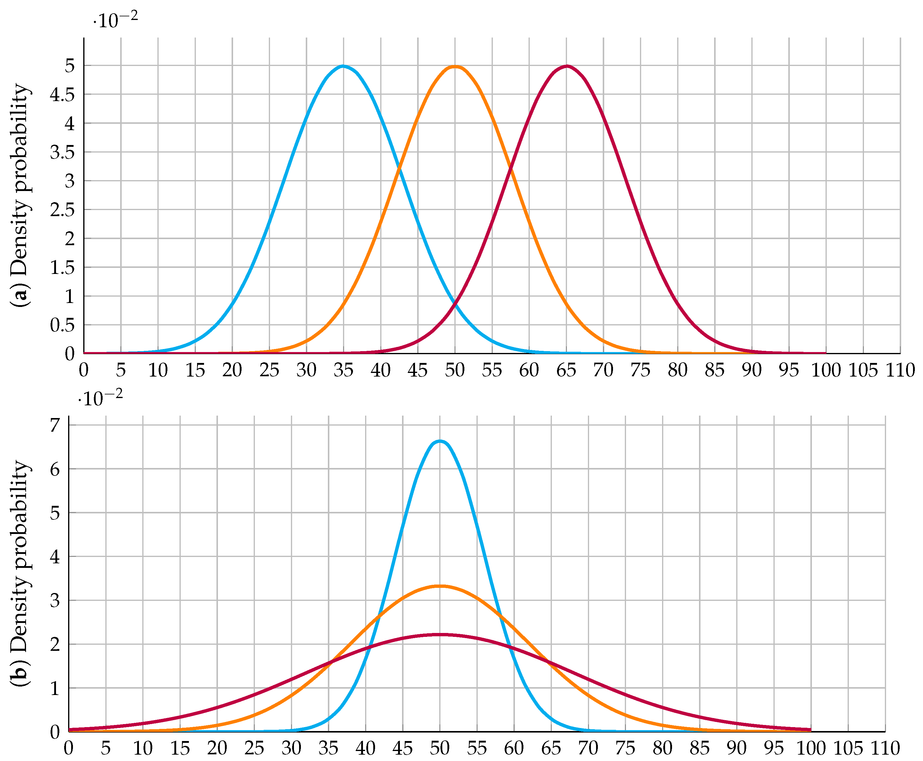
Note that parameters $\mu$ and $\delta$ determine the mean and standard deviation values of the random variables x. To illustrate the effect of these parameters in the behavior of Equation (13), Figure 1 presents the Gaussian distribution for different values of $\mu$ and $\delta$ [27].

In order to understand the behavior of the Gaussian distribution in Figure 1, note that (i) the movement of the Gaussian distribution is given by the direction of the increase in the $\mu$ parameter. At the same time, its standard deviation and amplitude remain constant due to the fixed value of the $\delta$ parameter (see Figure 1a); and (ii) the amplitude and standard deviation are modified when the $\delta$ parameter is changed, whereas the location of the Gaussian distribution remains fixed since the $\mu$ parameter is constant, as can be seen in Figure 1b).

Considering the advantage of Gaussian distributions in describing multiple physical and natural phenomena with a high level of precision, the author of [27] proposed an efficient and reliable optimization approach that combines the advantages of distribution probabilities with combinatorial optimization methods (population-based optimization algorithms).

The main features of the GNDO are listed below:

✔

An initial population is generated with a normal distribution throughout the solution space. This initial population evolves through the solution space to explore and exploit its promissory sub-regions. During the first stages of the optimization process, the variances regarding the positions of the solution individuals show minimal variations, and the location of the decision variables concerning the global optimal solution can be considered to be randomly distributed with a normal structure.

✔

As the evolution process through the solution space advances, the main position and the standard deviation are continuously decreased. This is done in order to pass from the exploration phase to the exploration of the solution space, i.e., refining the solution around the best solution reached.

✔

At the end of the optimization process, the variance of the positions between all the solution individuals and the distance between the mean position and the optimal solution reach minimum values.

Considering the characteristics mentioned above of the GNDO approach, the local and global exploration features of this optimization approach are presented below [24].

3.1.1. Local Exploration

Local exploration is typical of combinatorial optimization methods, where the population’s current solutions are evolving to find a better, optimal one. Considering the strong relationship between all solution individuals in the population in iteration t and the normal distribution, a generalized rule is defined for each individual, as presented in Equation (14):

$$\begin{array}{c}\hfill v_i^t={\mu }_i+{\delta }_i\eta ,i=1,2,\cdots ,N_i,\end{array}$$

(14)

where $v_i^t$ is the trailing vector of solution individual i in the current iteration; ${\mu }_i$ is the generalized mean location of individual i in iteration t; $\delta$ represents its generalized standard deviation; and $\eta$ is defined as a penalization factor. Note that $N_i$ is the total number of solutions in the population; each one of the individuals is generated in the form presented in Equation (15), which shows the general codification used to determine the nodes and the optimal sizes of the PV generators to be installed in the monopolar distribution network).

$$\begin{array}{c}\hfill x_i^t=\left[7,k,\cdots ,25|2.3006,p_k^{pv},\cdots ,1.2235\right]\end{array}$$

(15)

It is worth mentioning that, with this codification, the values of the objective function regarding the costs of the PV sources and their operation $z_2$ and $z_3$ are easily obtained.

Note that, in Equation (14), the parameters ${\mu }_i$, ${\delta }_i$, and $\eta$ are obtained using Equations (16) and (18).

$$\begin{array}{c}\hfill {\mu }_i=\frac{1}{3}\left(x_i^t+x_{\mathrm{best}}^t+M\right),\end{array}$$

(16)

$$\begin{array}{c}\hfill {\delta }_i=\frac{1}{\sqrt{3}}{\left({\left(x_i^t-\mu \right)}^2+{\left(x_{\mathrm{best}}^t-\mu \right)}^2+{\left(M-\mu \right)}^2\right)}^{\frac{1}{2}},\end{array}$$

(17)

$$\begin{array}{c}\hfill \eta =\left\{\begin{array}{ccc}{\left(-\log \left({\lambda }_1\right)\right)}^{\frac{1}{2}}cos\left(2\pi {\lambda }_2\right)& \mathrm{if}& a\le b\\ {\left(-\log \left({\lambda }_1\right)\right)}^{\frac{1}{2}}cos\left(2\pi {\lambda }_2+\pi \right)& \mathrm{if}& a>b\end{array}\right.\end{array}$$

(18)

In Equations (16)–(18), the parameters a, b, ${\lambda }_1$, and ${\lambda }_2$ are values in the range between 0 and 1, generated with a uniform distribution. In addition, $x_{\mathrm{best}}^t$ represents the best solution reached so far, and M corresponds to a vector that contains the mean position of the current individuals in the population. The way to calculate M is presented in Equation (19).

$$\begin{array}{c}\hfill M=\frac{1}{N_i}\sum _{i=1}^{N_i}{x}_i^t.\end{array}$$

(19)

3.1.2. Global Exploration

In combinatorial optimization, global exploration means using advanced evolution rules to explore the solution space and find promissory solution regions that are likely to harbor the global optimal solution [29]. In the GNDO approach, based on the recommendations of [27], the global exploration stage has three main components, which are combined in Equation (20).

$$\begin{array}{c}\hfill v_i^t=x_i^t+\beta \times \left(|{\lambda }_3|\times v_1\right)+\left(1-\beta \right)\times \left(|{\lambda }_4|\times v_2\right),\end{array}$$

(20)

where $\beta \times \left(|{\lambda }_3|\times v_1\right)$ has information regarding the local solution region, and $\left(1-\beta \right)\times \left(|{\lambda }_4|\times v_2\right)$ has information of the global solution space. Note that ${\lambda }_3$ and ${\lambda }_4$ represent random numbers obtained using a normal distribution, $\beta$ corresponds to a randomly chosen adjusting parameter between 0 and 1, and $v_1$ and $v_2$ are also two trail vectors.

$$\begin{array}{c}\hfill v_1=\left\{\begin{array}{ccc}{x}_i^t-x_j^t& \mathrm{if}& A_f\left(x_i^t\right)<A_f\left(x_j^t\right)\\ x_j^t-x_i^t& & \mathrm{otherwise}\end{array}\right.\end{array}$$

(21)

$$\begin{array}{c}\hfill v_2=\left\{\begin{array}{ccc}{x}_k^t-x_k^t& \mathrm{if}& A_f\left(x_k^t\right)<A_f\left(x_m^t\right)\\ x_m^t-x_k^t& & \mathrm{otherwise}\end{array}\right.\end{array}$$

(22)

Note that in Equations (21) and (22), the subscripts j, k, and m represent integer numbers associated with three positions of the solutions in the current population. The only restriction applicable to these numbers is that they must be different from each other and the analyzed individual i.

Before deciding whether the potential solution individual $v_i^t$ will be part of the next population, each one of the elements must be checked in order to ensure the feasibility of the solution, i.e.,

$$\begin{array}{c}\hfill v_{i,l}^t=\left\{\begin{array}{ccc}{v}_{i,l}^t& \mathrm{if}& x_l^{min}\le v_{i,l}^t\le x_l^{max}\\ v_{i,l}^t=x_l^{min}+{\lambda }_5\left(x_l^{max}-x_l^{min}\right)& & \mathrm{otherwise}.\end{array}\right.\end{array}$$

(23)

where $x_j^{min}$ and $x_j^{max}$ are the lower and upper admissible limits of the variable j, respectively. Note that, due to the restriction implied by the integer nature of the decision variables associated with the nodes where the PV sources are to be located, the first $N_{pv}^{ava}$ is rounded to its nearest integer value. In order to choose the next solution individual, the following rule is applied:

$$\begin{array}{c}\hfill x_i^{t+1}=\left\{\begin{array}{ccc}{v}_i^t& \mathrm{if}& A_f\left(v_i^t\right)<A_f\left(x_i^t\right)\\ x_i^t& & \mathrm{otherwise}\end{array}\right.\end{array}$$

(24)

3.2. Power Flow Solution

The power flow problem in electrical engineering is nonlinear and associated with determining the voltage variables in electrical systems under steady-state operating conditions [30]. In the case of the optimal siting and sizing of PV generation units in monopolar DC networks, the power flow solution is the fundamental key to determining the total energy purchasing costs at terminals of the substation [24]. In this research, the power flow solution technique implemented is the successive approximation method reported in [22].

The general power flow formula for the successive approximation power flow method is given in Equation (25).

$$\begin{array}{c}\hfill V_{d,h}^{m+1}=Y_{dd}^{-1}\left[{diag}^{-1}\left(V_{d,h}^m\right)\left(P_{pv,h}-P_{d,h}\right)-Y_{ds}{V}_{s,h}\right],\end{array}$$

(25)

where m is the counter assigned to the power flow iterations; $V_d$ is a vector that contains all the demanded voltage variables for each period h; $P_{pv,h}$ corresponds to a vector that contains the power outputs in the PV generators for each period h; $P_{d,h}$ represents a vector that contains all the power consumption in the load nodes for each period h; $V_{s,h}$ is the voltage output at the substation bus at any period; $Y_{dd}$ contains all the conductance relations among load nodes, which is a square invertible matrix; $Y_{ds}$ represents a rectangular matrix that associates the substation bus with the load nodes; and $diag\left(u\right)$ corresponds to a diagonal matrix composed of the elements of the u vector.

To determine whether the power flow Formula (25) has converged to the power flow solution, the difference between the voltage magnitudes of two continuous iterations is evaluated as defined in Equation (26).

$$\begin{array}{c}\hfill \underset{h}{max}\left\{\left|\right|V_{d,h}^{m+1}|-|V_{d,h}^m\left|\right|\right\}\le \gamma ,\end{array}$$

(26)

where $\gamma$ represents the maximum convergence error, i.e., $\gamma =1\times {10}^{-10}$ [22].

Once the power flow problem is solved by reaching the desired convergence, the power flow generation in the substation bus is obtained via Equation (27).

$$\begin{array}{c}\hfill P_{s,h}^{sub}=\left\{diag\left(V_{s,h}\right)\left(Y_{ss}{V}_{s,h}+Y_{sd}{V}_{d,h}\right)\right\}.\end{array}$$

(27)

Note that, with the power generation values at the substation bus, which are given by Equation (27), the component of the objective function $z_1$ is obtained. One of the most important aspects of combinatorial optimization is that it uses a fitness function to replace the original objective function, thus enabling the exploration of infeasible solution regions in the search for better objective function values (which increases the probabilities of finding the global optimum) [31,32]. The proposed fitness function for the studied problem takes the following structure.

$$\begin{array}{c}\hfill A_f=z_{\mathrm{cost}}+\left[\begin{array}{c}{\gamma }_1\underset{h}{max}\left\{|V_{d,h}|-v_d^{max},0\right\}+{\gamma }_2\underset{h}{max}\left\{|v_d^{min}-\left|V_{d,h}\right|,0\right\}-\\ {\gamma }_3\underset{h}{min}\left\{P_{s,h}^{sub},0\right\}-{\gamma }_4\underset{kj,h}{min}\left\{i_{kj}^{max}-\left|i_{kj,h}\right|,0\right\}\end{array}\right],\end{array}$$

(28)

Note that, in $A_f$, the parameters ${\gamma }_1$, ${\gamma }_2$, ${\gamma }_3$, and ${\gamma }_4$ correspond to the penalization factors of the objective function. These factors are activated in case the voltage regulation limits the maximum admissible current flow in the lines, or the positive semi-definite power generation requirements in a slack source are violated. Based on the recommendations of [24], the magnitude of said factors is selected as $100\times {10}^3$.

The main characteristic of the fitness function defined in Equation (28) is that when all the constraints of the optimization model (1)–(11) are fulfilled, the $A_f$ value is equal to the objective function, i.e., the global optimum the solution that guides the GNDO in the exploration and exploitation of the solution space is indeed the optimal solution of the MINLP model of Equations (1)–(11).

3.3. Summary of the Optimization Methodology

The application of the GNDO approach to solve the MINLP model defined from Equations (1)–(11) is summarized in Algorithm 1.

Note that the application of Algorithm 1 is general for any optimization problem. Nevertheless, two modifications are necessary to adapt the GNDO approach to multiple engineering optimization problems: (i) selecting the adequate codification of the studied problem and (ii) modifying the slave stage for the adequate fitness function evaluator.

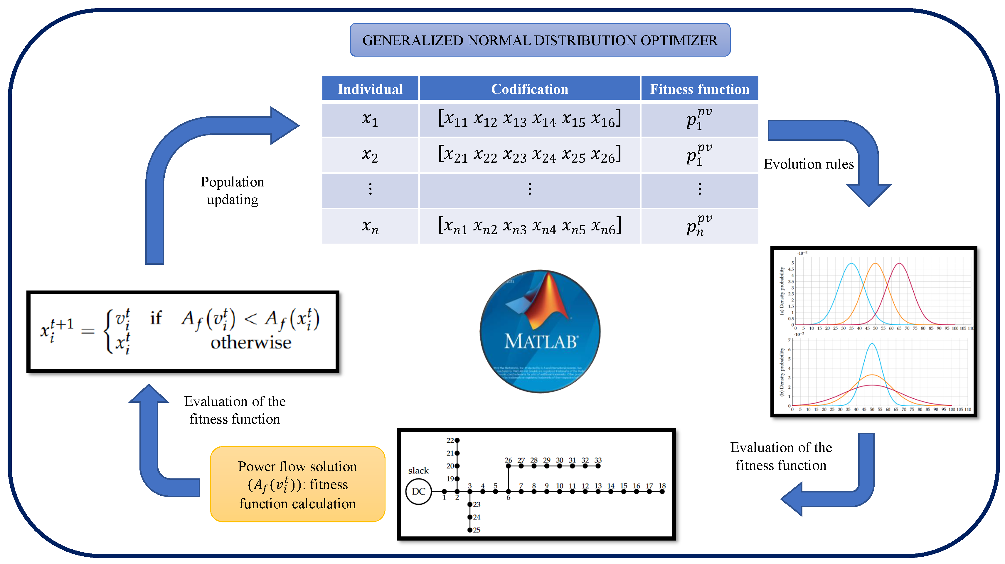
Figure 2 illustrates the general implementation of the proposed GNDO approach to locate and size PV sources in monopolar DC networks. Note that the codification is carried out using matrix representation, and power flow evaluation is performed via a power flow function also implemented in the MATLAB coding.   

Algorithm 1: Application of the GNDO method to locate and size PV sources in monopolar DC networks.

4. Test Feeder Characteristics and Problem Parametrization

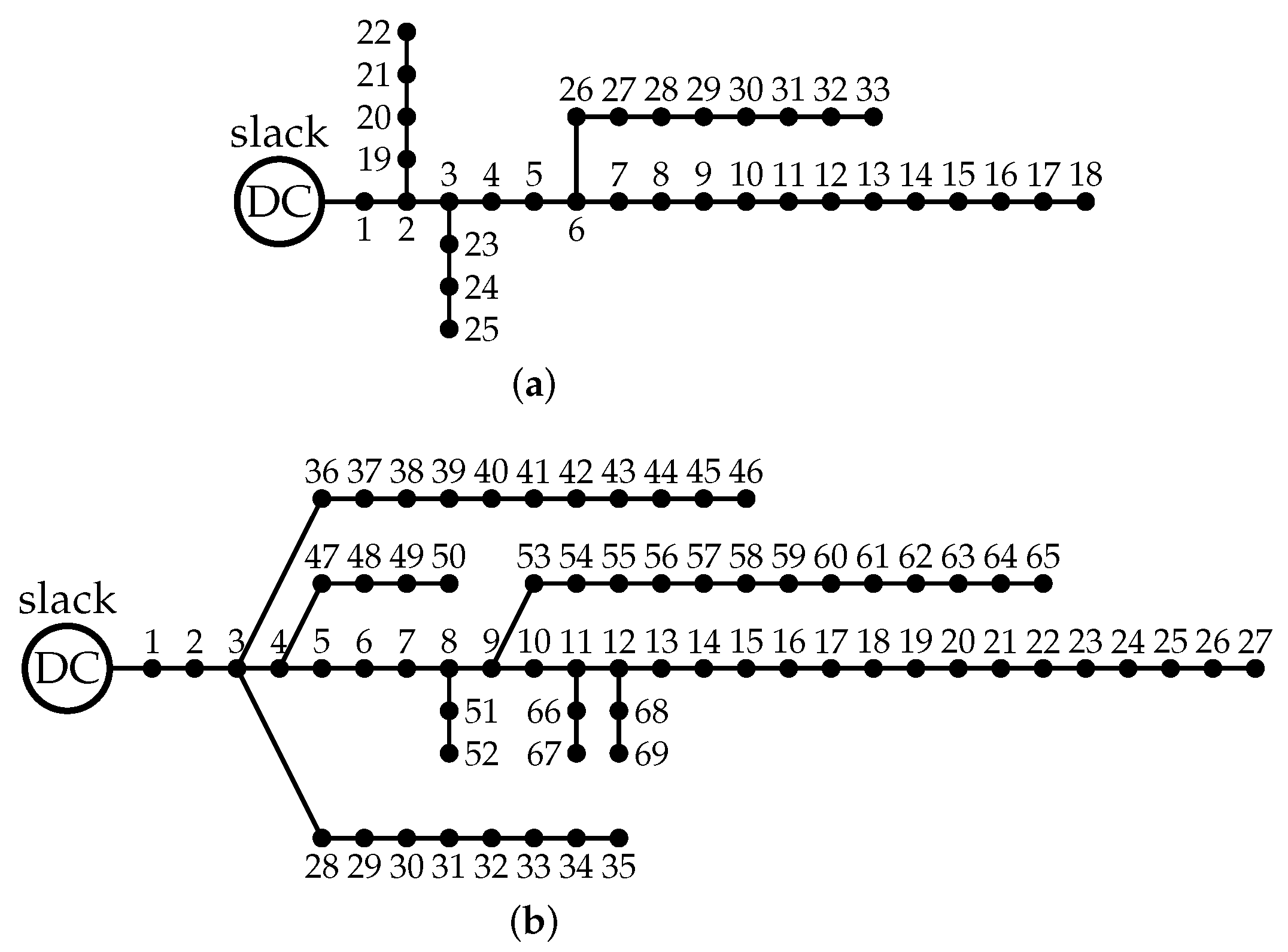
To study the problem regarding the optimal placement and sizing of PV generation sources in monopolar DC networks, two test feeders composed of 33 and 69 nodes were considered [22]. These systems correspond to the DC monopolar adaptation of the classical IEEE 33- and IEEE 69-bus grids [17].

4.1. First Test Feeder

The electrical configuration of the 33-bus grid is depicted in Figure 3a. This system’s main characteristic is that it operates with a monopolar DC voltage of $12.66$ kV between the positive pole and the return wire. All the branch and load parameters of this test feeder are listed in

Table 1. First test feeder, composed of 33 nodes.

Node i	Node j	${\mathit{R}}_{\mathbf{ij}}$ ($\mathbf{\Omega }$)	${\mathit{P}}_{\mathit{j}}$ (kW)	Node i	Node j	${\mathit{R}}_{\mathbf{ij}}$ ($\mathbf{\Omega }$)	${\mathit{P}}_{\mathit{j}}$ (kW)
1	2	0.0922	100	17	18	0.7320	90
2	3	0.4930	90	2	19	0.1640	90
3	4	0.3660	120	19	20	1.5042	90
4	5	0.3811	60	20	21	0.4095	90
5	6	0.8190	60	21	22	0.7089	90
6	7	0.1872	200	3	23	0.4512	90
7	8	1.7114	200	23	24	0.8980	420
8	9	1.0300	60	24	25	0.8960	420
9	10	1.0400	60	6	26	0.2030	60
10	11	0.1966	45	26	27	0.2842	60
11	12	0.3744	60	27	28	1.0590	60
12	13	1.4680	60	28	29	0.8042	120
13	14	0.5416	120	29	30	0.5075	200
14	15	0.5910	60	30	31	0.9744	150
15	16	0.7463	60	31	32	0.3105	210
16	17	1.2860	60	32	33	0.3410	60

.

4.2. Second Test Feeder

The electrical configuration of the 69-bus grid is depicted in Figure 3b. This system’s main characteristic is that it operates with a monopolar DC voltage of $12.66$ kV between the positive pole and the return wire. All the branch and load parameters for this test feeder are listed in

Table 2. Second test feeder, composed of 69 nodes.

Node i	Node j	${\mathit{R}}_{\mathbf{ij}}$ ($\mathbf{\Omega }$)	${\mathit{P}}_{\mathit{j}}$ (kW)	Node i	Node j	${\mathit{R}}_{\mathbf{ij}}$ ($\mathbf{\Omega }$)	${\mathit{P}}_{\mathit{j}}$ (kW)
1	2	0.0005	0	3	36	0.0044	26
2	3	0.0005	0	36	37	0.0640	26
3	4	0.0015	0	37	38	0.1053	0
4	5	0.0251	0	38	39	0.0304	24
5	6	0.3660	2.6	39	40	0.0018	24
6	7	0.3810	40.4	40	41	0.7283	1.2
7	8	0.0922	75	41	42	0.3100	0
8	9	0.0493	30	42	43	0.0410	6
9	10	0.8190	28	43	44	0.0092	0
10	11	0.1872	145	44	45	0.1089	39.22
11	12	0.7114	145	45	46	0.0009	39.22
12	13	1.0300	8	4	47	0.0034	0
13	14	1.0440	8	47	48	0.0851	79
14	15	1.0580	0	48	49	0.2898	384.7
15	16	0.1966	45.5	49	50	0.0822	384.7
16	17	0.3744	60	8	51	0.0928	40.5
17	18	0.0047	60	51	52	0.3319	3.6
18	19	0.3276	0	9	53	0.1740	4.35
19	20	0.2106	1	53	54	0.2030	26.4
20	21	0.3416	114	54	55	0.2842	24
21	22	0.0140	5	55	56	0.2813	0
22	23	0.1591	0	56	57	1.5900	0
23	24	0.3460	28	57	58	0.7837	0
24	25	0.7488	0	58	59	0.3042	100
25	26	0.3089	14	59	60	0.3861	0
26	27	0.1732	14	60	61	0.5075	1244
3	28	0.0044	26	61	62	0.0974	32
28	29	0.0640	26	62	63	0.1450	0
29	30	0.3978	0	63	64	0.7105	227
30	31	0.0702	0	64	65	1.0410	59
31	32	0.3510	0	11	66	0.2012	18
32	33	0.8390	14	66	67	0.0047	18
33	34	1.7080	19.5	12	68	0.7394	28
34	35	1.4740	6	68	69	0.0047	28

.

4.3. Parametrization of the Studied Problem

To determine the objective function value and calculate the fitness function, all the parameters in

Table 3. Fitness and objective function parametrization.

Parameter	Value	Unit	Parameter	Value	Unit
$C_{\mathrm{kWh}}$	0.1390	US$/kWh	T	365	days
$t_a$	10	%	$t_e$	2	%
y	20	years	$\Delta h$	1	h
$C_{\mathrm{PV}}$	1036.49	US$/kWp	$C_{O\&M}$	0.0019	US$/kWh
$p_i^{pv,max}$	2400	kW	$p_i^{pv,min}$	0	kW
$N_{pv}^{ava}$	3	–	$\Delta V$	±10	%
${\gamma }_1$	$100\times {10}^3$	US$/V	${\gamma }_2$	$100\times {10}^3$	US$/V
${\gamma }_3$	$100\times {10}^3$	US$/W	${\gamma }_4$	$100\times {10}^3$	US$/A

were employed [22].

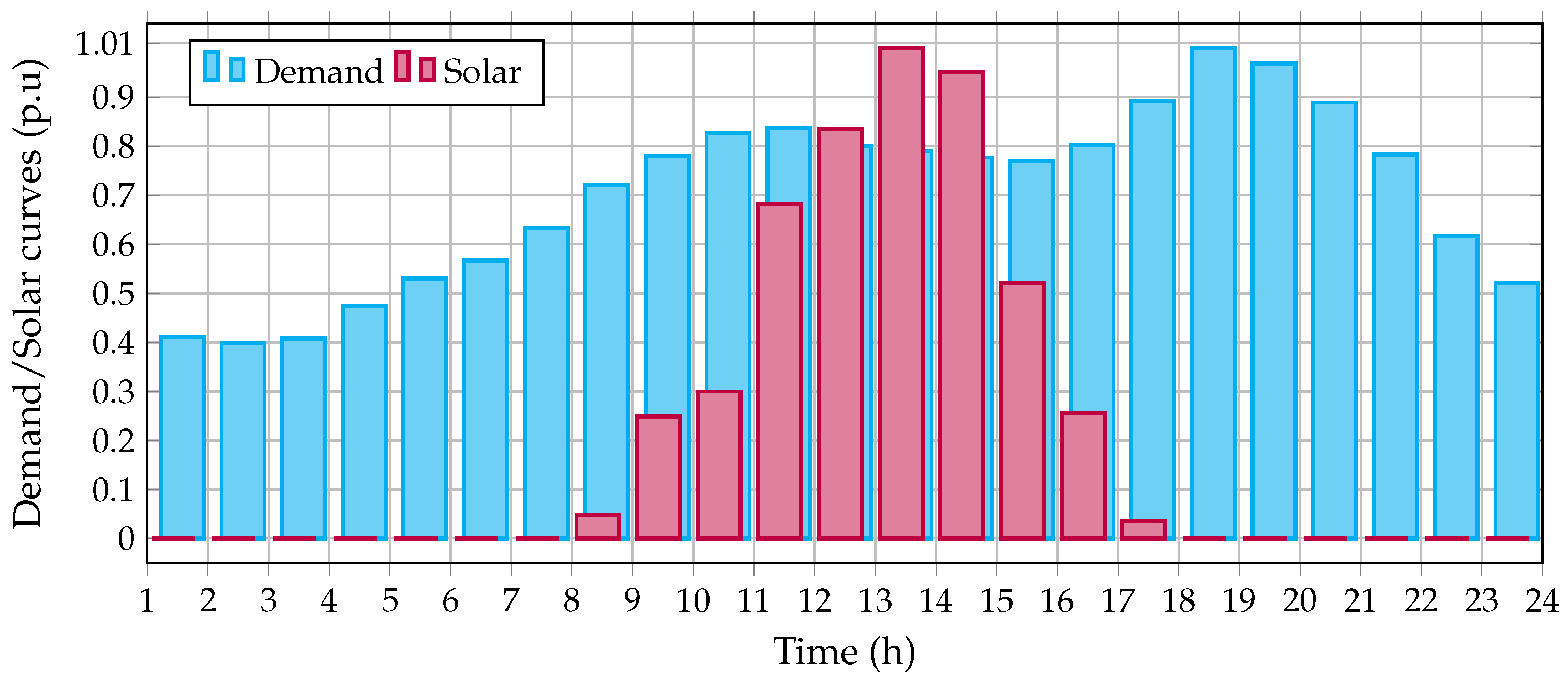
On the other hand, in order to evaluate the expected daily behavior of the monopolar DC networks under study, this research considered the generation and demand curves of Medellín, Colombia, as depicted in Figure 4. These curves were adapted from [24]. It is worth mentioning that Colombia is a non-seasonal country, which implies that the average yearly demand and solar generation curves are enough for installing PV generation units.

Remark 2.

Our contribution considers the expected power generation from the solar source in the typical metropolitan area of Medellín, Colombia. The maximum size considered for the solar sources is 2400 kW. Due to the fact that it is a planning project, the expected generation curve is taken into account. This curve was calculated using historical data (1 year) for this city with an hourly resolution. A recursive artificial neural network was used to determine the expected daily behavior.

5. Computational Validation

Two efficient metaheuristics were used to show the efficiency of the proposed GNDO algorithm at locating and sizing PV generation units in monopolar DC distribution networks. The metaheuristics were the Chu and Beasley genetic algorithm (AGCB) and the discrete-continuous vortex search algorithm (DCVSA) [22]. The computational implementation of the metaheuristic optimizers was carried out in MATLAB using our scripts. Regarding the software, Matlab version R2021b was used in the 64-bits version of Microsoft Windows. Hardware-wise, an Intel(R) Core(TM) i7–7700HQ CPU 2.80 GHz computer with 24 GB of RAM was used.

A population size of 10 individuals, 1000 iterations, and 100 repetitions of each algorithm was used in order to make an adequate comparison between the proposed GNDO approach and the CGBA and the DCVSA.

5.1. Results for the First Test Feeder

Table 4. Application of the GNDO approach to the location and sizing of PV generation in the 33-bus grid and comparison of results with literature reports.

Method	Site (Node)/Size (kW)	${\mathit{z}}_{\mathbf{cost}}$ (US$/Year)
Bench. case	–	3,644,043.01
CBGA	$\left\{\begin{array}{c}11\left(1162.95\right),14\left(943.48\right),31\left(1482.75\right)\end{array}\right\}$	2,662,724.82
DCVSA	$\left\{\begin{array}{c}9\left(580.31\right),15\left(1291.37\right),31\left(1715.59\right)\end{array}\right\}$	2,662,425.32
GNDO	$\left\{\begin{array}{c}10\left(974.26\right),16\left(920.22\right),31\left(1692.51\right)\end{array}\right\}$	2,662,371.59

presents the numerical results in the 33-bus grid when the proposed and comparative metaheuristics were implemented.

The numerical results in Table 4 show the following:

✔

The reduction concerning the benchmark case with the CBGA was about USD/year 981,318.19, which corresponds to $26.9294\%$. The reduction reached with the DCVSA was about USD/year 981,617.69, ($26.9376\%$), and the best solution for the benchmark case was reached with the proposed GNDO approach, with USD/year 981,671.42, i.e., a reduction of $26.9391\%$. These results show that all the optimizers yield an annual expected reduction of USD 981,300.00 per year of operation. Furthermore, comparing the best literature report (solution with the DCVSA in [22] with the proposed GNDO approach, an improvement of about USD/year 53.73 is achieved, which makes it the best result reported in the current literature for the 33-bus grid with a DC monopolar configuration.

✔

The three algorithms detected that one of the best sites to locate a PV source is node 31, where injections of power higher than 1540 kW are listed. This location demonstrates that the 33-bus grid is one of the most sensitive nodes to install PV sources concerning the expected improvement of the objective function. In addition, the total PV capacity installed with the CBGA is $3589.18$ kW, $3587.27$ kW with the DCVSA, and $3586.99$ kW with the proposed GNDO. These values show that, for the 33-bus grid, the proposed GNDO installed less power with better objective function values, which a better nodal selection can explain in comparison with the CBGA and the DCVSA.

As for the processing times, it is worth mentioning that the proposed GNDO approach takes an average time of 159.99 s to solve the studied problem, which shows that for solving a nonlinear programming model with integer and continuous variables (solution space with infinite dimensions), the proposed GNDO approach takes less than 3 min. This implies that a utility company can use this approach to evaluate hundreds of nodal locations for PV generation units with lower processing times in order to find an adequate solution from both economic and technical perspectives.

5.2. Results for the Second Test Feeder

Table 5. Application of the GNDO approach to the location and sizing of PV generation in the 69-bus grid and comparison of results with literature reports.

Method	Site (Node)/Size (kW)	${\mathit{z}}_{\mathbf{cost}}$ (US$/Year)
Bench. case	–	3,817,420.38
CBGA	$\left\{\begin{array}{c}19\left(790.80\right),61\left(1789.05\right),64\left(1147.42\right)\end{array}\right\}$	2,785,598.86
DCVSA	$\left\{\begin{array}{c}23\left(772.01\right),62\left(2340.27\right)63\left(618.53\right)\end{array}\right\}$	2,785,538.58
GNDO	$\left\{\begin{array}{c}19\left(497.00\right),61\left(2399.99\right),64\left(847.04\right)\end{array}\right\}$	2,785,011.53

shows the numerical results in the 69-bus grid when the proposed and comparative metaheuristics were implemented.

The results in Table 5 allow observing the following:

✔

The proposed GNDO approach achieves the best reduction with respect to the benchmark case, with a value of USD/year 1,032,408.85, i.e., $27.044\%$. The DCVSA reached an annual reduction of USD/year 1,031,881.8, corresponding to an improvement of $27.0309\%$, and the CBGA reduced the expected annual operating costs by about USD/year 1,031,821.52, i.e., $27.0293\%$ with respect of the benchmark case.

✔

The nodes to locate PV generators for the proposed GNDO and the CBGA are the same, i.e., nodes 19, 61, and 64. However, the sizes assigned to the PV sources in these nodes differ between them. This behavior is explained by using the Gaussian distribution functions and decreasing the radius in the GNDO approach, which allows shifting from exploring the solution space to exploiting it.

✔

The improvement obtained with the GNDO with respect to the CBGA was USD 587.33 per year of operation, whereas, for the DCVSA, this improvement was about USD/year $527.05$. These results demonstrate that the proposed master–slave optimizer is the best current solution reported for the 69-bus DC network with a monopolar configuration, i.e., the GNDO represents the reference point for future research in this area.

It is worth mentioning that the proposed GNDO approach takes about $376.88$ s to solve the problem regarding the optimal placement and sizing of PV sources in monopolar DC distribution networks, i.e., it takes less than 6.5 min to solve a highly complex optimization problem with excellent numerical results.

6. Conclusions and Future Work

This research addressed the problem concerning the optimal placement and sizing of PV generation units in monopolar DC distribution grids with a radial structure by applying a master–slave optimization approach. In the master stage, the GNDO approach was used to define the nodal location and sizes of the PV sources by using a discrete-continuous codification, whereas the slave stage corresponded to an efficient DC power flow approach that allowed evaluating the fitness function. Numerical results in the DC monopolar versions of the IEEE 33- and IEEE 69-bus grids demonstrate that the GNDO approach allowed reaching better results than the DCVSA with reductions of USD/year 53.73, and USD/year 527.05, respectively, which turns the proposed master–slave approach into the best current reference regarding the studied problem.

As for the processing times, the proposed GNDO approach took less than 3 and 6.5 min to solve the MINLP model (1)–(12) in test feeders with 33 and 69 nodes, respectively. These results implied discrete solution spaces of 4960 and 50,116 nodal combinations and infinite possibilities regarding continuous variables, yielding the best numerical results in connection with the objective function when compared to those of the CBGA and the DCVSA.

The main limitation of the proposed optimization approach corresponds to the design of the PV systems, taking into account that these operate by tracking the maximum power point. However, it is possible to obtain better objective function values if these PV sources are freely operated, i.e., under a multi-period, optimal power flow design.

As future works, the following work could be carried out: (i) extending the application of the GNDO approach in order to solve the problem of the optimal selection, location, and operation of batteries in AC and DC distribution grids; and (ii) transforming the exact MINLP model (1)–(12) into a mixed-integer conic formulation that allows determining the best set of nodes and their optimal sizes via convex programming.

References

- Li, J.; Liu, F.; Wang, Z.; Low, S.H.; Mei, S. Optimal Power Flow in Stand-Alone DC Microgrids. IEEE Trans. Power Syst. 2018, 33, 5496–5506. [Google Scholar] [CrossRef] [Green Version]
- Garces, A. On the Convergence of Newton’s Method in Power Flow Studies for DC Microgrids. IEEE Trans. Power Syst. 2018, 33, 5770–5777. [Google Scholar] [CrossRef] [Green Version]
- Strzelecki, R.M.; Benysek, G. (Eds.) Power Electronics in Smart Electrical Energy Networks; Springer: London, UK, 2008. [Google Scholar] [CrossRef]
- Junior, M.E.T.S.; Freitas, L.C.G. Power Electronics for Modern Sustainable Power Systems: Distributed Generation, Microgrids and Smart Grids—A Review. Sustainability 2022, 14, 3597. [Google Scholar] [CrossRef]
- Lee, J.O.; Kim, Y.S.; Jeon, J.H. Generic power flow algorithm for bipolar DC microgrids based on Newton–Raphson method. Int. J. Electr. Power Energy Syst. 2022, 142, 108357. [Google Scholar] [CrossRef]
- Lamb, W.F.; Grubb, M.; Diluiso, F.; Minx, J.C. Countries with sustained greenhouse gas emissions reductions: An analysis of trends and progress by sector. Clim. Policy 2021, 22, 1–17. [Google Scholar] [CrossRef]
- Lima, M.; Mendes, L.; Mothé, G.; Linhares, F.; de Castro, M.; da Silva, M.; Sthel, M. Renewable energy in reducing greenhouse gas emissions: Reaching the goals of the Paris agreement in Brazil. Environ. Dev. 2020, 33, 100504. [Google Scholar] [CrossRef]
- López, A.R.; Krumm, A.; Schattenhofer, L.; Burandt, T.; Montoya, F.C.; Oberländer, N.; Oei, P.Y. Solar PV generation in Colombia—A qualitative and quantitative approach to analyze the potential of solar energy market. Renew. Energy 2020, 148, 1266–1279. [Google Scholar] [CrossRef]
- Cuervo, F.I.; Arredondo-Orozco, C.A.; Marenco-Maldonado, G.C. Photovoltaic power purchase agreement valuation under real options approach. Renew. Energy Focus 2021, 36, 96–107. [Google Scholar] [CrossRef]
- Moradi, M.H.; Abedini, M. A combination of genetic algorithm and particle swarm optimization for optimal DG location and sizing in distribution systems. Int. J. Electr. Power Energy Syst. 2012, 34, 66–74. [Google Scholar] [CrossRef]
- Paz-Rodríguez, A.; Castro-Ordoñez, J.F.; Montoya, O.D.; Giral-Ramírez, D.A. Optimal integration of photovoltaic sources in distribution networks for daily energy losses minimization using the vortex search algorithm. Appl. Sci. 2021, 11, 4418. [Google Scholar] [CrossRef]
- Selim, A.; Kamel, S.; Alghamdi, A.S.; Jurado, F. Optimal placement of DGs in distribution system using an improved harris hawks optimizer based on single-and multi-objective approaches. IEEE Access 2020, 8, 52815–52829. [Google Scholar] [CrossRef]
- Mohanty, B.; Tripathy, S. A teaching learning based optimization technique for optimal location and size of DG in distribution network. J. Electr. Syst. Inf. Technol. 2016, 3, 33–44. [Google Scholar] [CrossRef] [Green Version]
- Ayodele, T.; Ogunjuyigbe, A.; Akinola, O. Optimal location, sizing, and appropriate technology selection of distributed generators for minimizing power loss using genetic algorithm. J. Renew. Energy 2015, 2015, 832917. [Google Scholar] [CrossRef] [Green Version]
- Raharjo, J.; Adam, K.B.; Priharti, W.; Zein, H.; Hasudungan, J.; Suhartono, E. Optimization of Placement and Sizing on Distributed Generation Using Technique of Smalling Area. In Proceedings of the 2021 IEEE Electrical Power and Energy Conference (EPEC), Toronto, ON, Canada, 22–31 October 2021; pp. 475–479. [Google Scholar]
- Grisales-Noreña, L.F.; Gonzalez Montoya, D.; Ramos-Paja, C.A. Optimal sizing and location of distributed generators based on PBIL and PSO techniques. Energies 2018, 11, 1018. [Google Scholar] [CrossRef] [Green Version]
- Kaur, S.; Kumbhar, G.; Sharma, J. A MINLP technique for optimal placement of multiple DG units in distribution systems. Int. J. Electr. Power Energy Syst. 2014, 63, 609–617. [Google Scholar] [CrossRef]
- Montoya, O.D.; Grisales-Noreña, L.F.; Gil-González, W.; Alcalá, G.; Hernandez-Escobedo, Q. Optimal location and sizing of PV sources in DC networks for minimizing greenhouse emissions in diesel generators. Symmetry 2020, 12, 322. [Google Scholar] [CrossRef] [Green Version]
- Gil-González, W.; Montoya, O.D.; Grisales-Noreña, L.F.; Perea-Moreno, A.J.; Hernandez-Escobedo, Q. Optimal placement and sizing of wind generators in AC grids considering reactive power capability and wind speed curves. Sustainability 2020, 12, 2983. [Google Scholar] [CrossRef] [Green Version]
- Radosavljević, J.; Arsić, N.; Milovanović, M.; Ktena, A. Optimal placement and sizing of renewable distributed generation using hybrid metaheuristic algorithm. J. Mod. Power Syst. Clean Energy 2020, 8, 499–510. [Google Scholar] [CrossRef]
- Gil-González, W.; Garces, A.; Montoya, O.D.; Hernández, J.C. A mixed-integer convex model for the optimal placement and sizing of distributed generators in power distribution networks. Appl. Sci. 2021, 11, 627. [Google Scholar] [CrossRef]
- Cortés-Caicedo, B.; Molina-Martin, F.; Grisales-Noreña, L.F.; Montoya, O.D.; Hernández, J.C. Optimal Design of PV Systems in Electrical Distribution Networks by Minimizing the Annual Equivalent Operative Costs through the Discrete-Continuous Vortex Search Algorithm. Sensors 2022, 22, 851. [Google Scholar] [CrossRef]
- Hlaili, M.; Mechergui, H. Comparison of Different MPPT Algorithms with a Proposed One Using a Power Estimator for Grid Connected PV Systems. Int. J. Photoenergy 2016, 2016, 1728398. [Google Scholar] [CrossRef] [Green Version]
- Montoya, O.D.; Grisales-Noreña, L.F.; Ramos-Paja, C.A. Optimal Allocation and Sizing of PV Generation Units in Distribution Networks via the Generalized Normal Distribution Optimization Approach. Computers 2022, 11, 53. [Google Scholar] [CrossRef]
- Farivar, M.; Low, S.H. Branch Flow Model: Relaxations and Convexification—Part I. IEEE Trans. Power Syst. 2013, 28, 2554–2564. [Google Scholar] [CrossRef]
- Crainic, T.G.; Toulouse, M. Parallel Meta-heuristics. In International Series in Operations Research & Management Science; Springer: Berlin/Heidelberg, Germany, 2010; pp. 497–541. [Google Scholar] [CrossRef]
- Zhang, Y.; Jin, Z.; Mirjalili, S. Generalized normal distribution optimization and its applications in parameter extraction of photovoltaic models. Energy Convers. Manag. 2020, 224, 113301. [Google Scholar] [CrossRef]
- Abdel-Basset, M.; Mohamed, R.; Abouhawwash, M.; Chang, V.; Askar, S. A Local Search-Based Generalized Normal Distribution Algorithm for Permutation Flow Shop Scheduling. Appl. Sci. 2021, 11, 4837. [Google Scholar] [CrossRef]
- Xu, J.; Zhang, J. Exploration-exploitation tradeoffs in metaheuristics: Survey and analysis. In Proceedings of the 33rd Chinese Control Conference, Nanjing, China, 28–30 July 2014. [Google Scholar] [CrossRef]
- Garces, A. Uniqueness of the power flow solutions in low voltage direct current grids. Electr. Power Syst. Res. 2017, 151, 149–153. [Google Scholar] [CrossRef]
- Sahin, O.; Akay, B. Comparisons of metaheuristic algorithms and fitness functions on software test data generation. Appl. Soft Comput. 2016, 49, 1202–1214. [Google Scholar] [CrossRef]
- Hanh, L.T.M.; Binh, N.T.; Tung, K.T. A Novel Fitness function of metaheuristic algorithms for test data generation for simulink models based on mutation analysis. J. Syst. Softw. 2016, 120, 17–30. [Google Scholar] [CrossRef]
Figure 1.
Variations in the Gaussian distribution as a function of the changes in the and parameters: (a) behavior of the Gaussian distribution when is fixed, and is varied; (b) behavior of the Gaussian distribution when is fixed, and is varied.
Figure 2.
General implementation of the GNDO approach in MATLAB software for the studied problem.
Figure 3.
Test feeder topologies: (a) 33-bus grid and (b) 69-bus grid.
Figure 4.
Daily demand and generation curves of Medellín, Colombia.