Experimental Measurement Benchmark for Compressible Fluidic Unsteady Jet


University Lille, CNRS, ONERA, Arts et Metiers Paris Tech, Centrale Lille, FRE2017–LMFL, Laboratoire de Mécanique des Fluides de Lille–Kampé de Fériet, F-59000 Lille, France
*
Author to whom correspondence should be addressed.
Actuators 2018, 7(3), 58; https://doi.org/10.3390/act7030058
Submission received: 23 July 2018
/
Revised: 20 August 2018
/
Accepted: 6 September 2018
/
Published: 10 September 2018
(This article belongs to the Special Issue Synthetic Jet Actuators)
Abstract
:A benchmark of different measurement techniques is presented to characterize the dynamic response of a synthetic jet actuator working in compressible regime. The setup involves a piston-based synthetic jet, as well as the benchmarked measurements are hot-wire, cold-wire, Laser Doppler Anemometry, pressure transducer, and Schlieren visualization. Measured flow temperatures range from 20 °C to 150 °C, pressure ranges from 0.5 atm to 4 atm, and velocity are up to 300 m/s. The extreme values of these ranges are reached in an oscillating fashion at a frequency ranging from 30 to 100 Hz. The measurements are pointing out the limitation of cold-wire measurements, due to its high thermic inertia. The results show consistency in the velocity measurements, within 10% in the worst case, between all measurement techniques and the errors are traced back to the calibration ranges, whose sensitivity is also studied.
Keywords:
compressible jet; measurements; calibration; synthetic-jet; hot-wire; cold-wire; LDA; Schlieren; shadowgraphy1. Introduction
In the compressible regime, the velocity and pressure fields are coupled to the thermodynamic state of the fluid. From an experimental standpoint, this implies that the characterization of a compressible fluid through indirect measurements is more challenging, since relations between the properties of interest become dependent on more variables than in their incompressible counterpart. Furthermore, all these variables should in rigor be measured simultaneously.
An illustrating example is the problem of determining the fluid velocity using pitot probes or hot-wires. In the case of pitot probes and in the incompressible regime, the pressure is measured, and a simple correlation exists through the Bernoulli or Saint Venant equations which allow calculating the velocity. However, in the compressible regime, the relations change and the pressure now correlates with the Mach number—a number which, unsurprisingly, involves an intrinsically thermodynamic variable, the speed of sound. A similar problem arises if one attempts to determine the fluid velocity using a hot-wire. In the incompressible regime, the fluid velocity correlates with the heat exchange between the electrically charged wire and the fluid, which in turn correlates with its electrical signal, allowing the measurement. However, in the weakly compressible regime, the heat exchange will depend on the Reynolds number—which involves a thermodynamic variable, the fluid density. Moreover, in the strongly compressible regime, the heat exchange will also depend on the Mach number. The compressible regime thus invalidates classical approaches for indirectly measuring the relevant magnitudes in fluid mechanics, and tailored relations and methods involving simultaneous measurements or further knowledge about the state of the fluid are required.
The objective of this work is to provide a benchmark of different instruments and techniques available to locally characterize an oscillating fluid in the compressible subsonic regime.
A review on the state of the art for time-resolved measurement probes at the beginning of this millennium is contained in Reference [1]. Techniques such as hot-wire anemometry, Laser Doppler anemometry and fast-response aerodynamics probes are compared in that article.
Hot-wire anemometry (HWA) aims to obtain the time-resolved local mass-flux. It is a quick accurate technique and requires an easy setup which, according to Reference [2], makes it one of the most widely used intrusive measurement techniques for velocity in fluctuating flows. However, measurements in compressible flows with a hot-wire are non-trivial, since as stated before correlations of their signal with physical magnitudes happen to be multifactorial. Most of the research to deal with that problem was made in the second half of the last century, beginning with Kovasznay’s milestone on the measurement in the supersonic and transonic regime [3]. A recent overview of the latest developments on the subject is contained in Reference [4]. More specific information on hot-wire metrology is also available in transonic [5] and supersonic [6] regimes.
A combination of hot-wire and cold-wire to characterize unsteady flows is used in [7], and is utilized in this study to compute the velocity output. On the analytical models for the estimation of mass flow rate, the reader can refer to the recent work of Zong and Kotsonis [8], on plasma synthetic jet actuators. Here, cold-wires generally lack the hot-wire’s fast time response, and their time response can be measured following Reference [9]. However, and up to 20 kHz, time-resolved temperature probes using the cold-wire concept are developed in Reference [10]. The calibration of hot-wires varies according to their regime, and can be done following Reference [11], and a revised approach in Reference [12].
Laser Doppler anemometry (LDA) in compressible flows offers the advantages of unambiguous signal interpretation, since the laser Doppler anemometer senses velocity only, and has the benefit of non-intrusiveness [13]. As explained in Reference [13], the accuracy of an LDA measurement is determined by the Signal-to-Noise Ratio (SNR), which depends on the lens, the size of the seeding particles, and the power of the laser. A trade-off exists in which the size should be small enough to follow the fluid lines, but large enough to be correctly sensed by the LDA without introducing much noise.
As the flow field visualization methods are concerned, an up-to-date thorough review of Schlieren and shadowgraph techniques can be accessed in Reference [14]. Both methods are qualitative, and their main advantage is their non-intrusiveness and their capability to visualize an entire field. The Schlieren technique allows measurement with continuity in time, while the shadowgraphy takes a number of discrete images within a very short time interval. Therefore, while the Schlieren method is useful to obtain insight on the flow dynamics, the shadowgraphy can uncover high-frequency phenomena, as used in this article.
In this paper, the benchmarking will be done over a synthetic jet, which can constitute a source of subsonic, transonic and supersonic flows. Moreover, since the applications of the synthetic jet are multiple, like flow control [15,16] or cooling [17,18], with significant research on this topic [19,20,21,22], this benchmark takes interest for both applied and theoretical experimental research. This choice also provides the possibility to test the measurements methodology validity for characterizing unsteady flows with fast response.
The techniques to be benchmarked are: Laser Doppler Anemometry, single-wire hot-wire, cold-wire, pressure transducer, Schlieren, and shadowgraphy visualization. Details can be found in [23].
This article is divided into three main sections: In Section 2, on experimental setup and instrumentation, the benchmark setup and the technical characterization of the various measurement instruments are described. In Section 3, the results and discussion section, the aforementioned techniques are used to characterize the synthetic jet and compared against each other. The article concludes with Section 4, on the perspectives and opportunities of future work that this article unlocks.
2. Experimental Setup and Instrumentation
In the following two subsections the experimental setup and instrumentation are presented.
2.1. Setup
The experiment is carried out in a workbench specifically designed to characterize fluidic actuators [24,25]. In this subsection, the geometry on which the experiments were carried out, and the different techniques are briefly introduced.
The synthetic jet actuator is comprised of a cavity open to the exterior by a circular orifice, and with one side moving thanks to an oscillating piston. The measured data considered are cavity pressure (unsteady Kulite sensor), ambient pressure (Druck sensor), output temperature (cold-wire), output velocity (LDA and hot-wire), output flow field (Schlieren), operating piston engine (tachymeter).
For the experiment, the different instruments are installed around the actuator. Except the cold-wire and hot-wire measurements, the others are performed individually, and not at the same time. Results from the different instruments are later synchronized to the piston cyclic motion for comparison purposes, since phenomena are periodic, due to a constant piston frequency.
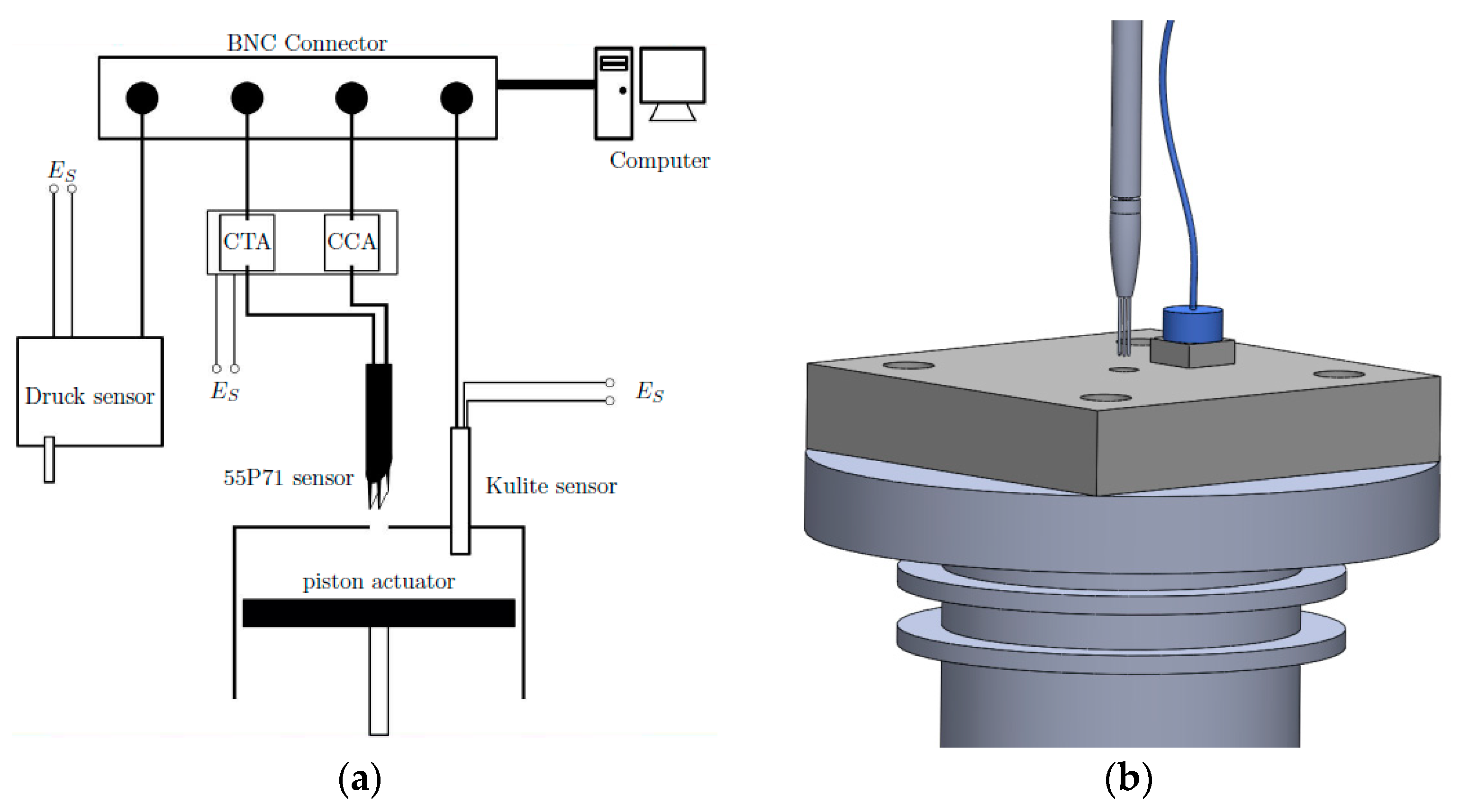
The jet module, including the transducer, the electric motor and the frequency sensor, is placed on the test bench. The supply tube for the parallel array wires is mounted on a multi-axis system, which allows adjusting the position of the wires before and during the measurement. The multi-axis system is driven by electric motors in the three directions which makes it possible to place the hot- and cold-wire precisely and to survey the spatially homogeneity of the jet flow. An internal LabVIEW tool is used to set the position of the multi-axis system. The Kulite sensor measuring the cavity chamber pressure is connected to the top orifice plate, and the Druck sensor that monitors the ambient pressure measurement is placed on the test bench next to the other equipment, to reduce the influence of the jet stream on the sensor. Figure 1 shows a schematic drawing of the measurement cycle with the main devices as sensors, the actuator and the connection to the computer unit. The sensors are connected to a BNC2090 module, also shown in Figure 1. The connector is then linked to a computer. The data acquisition system is comprised of two National Instrument DAQ cards, NI PCI-6123 and NI-PCI-6120. With an in house LabVIEW program, the sensors voltage can be recorded during the measurement.
All measurement equipment’s are certified, verified and connected to the metrological laboratory of ONERA Lille center, itself connected to the national primary standards.
2.1.1. Actuator Geometry
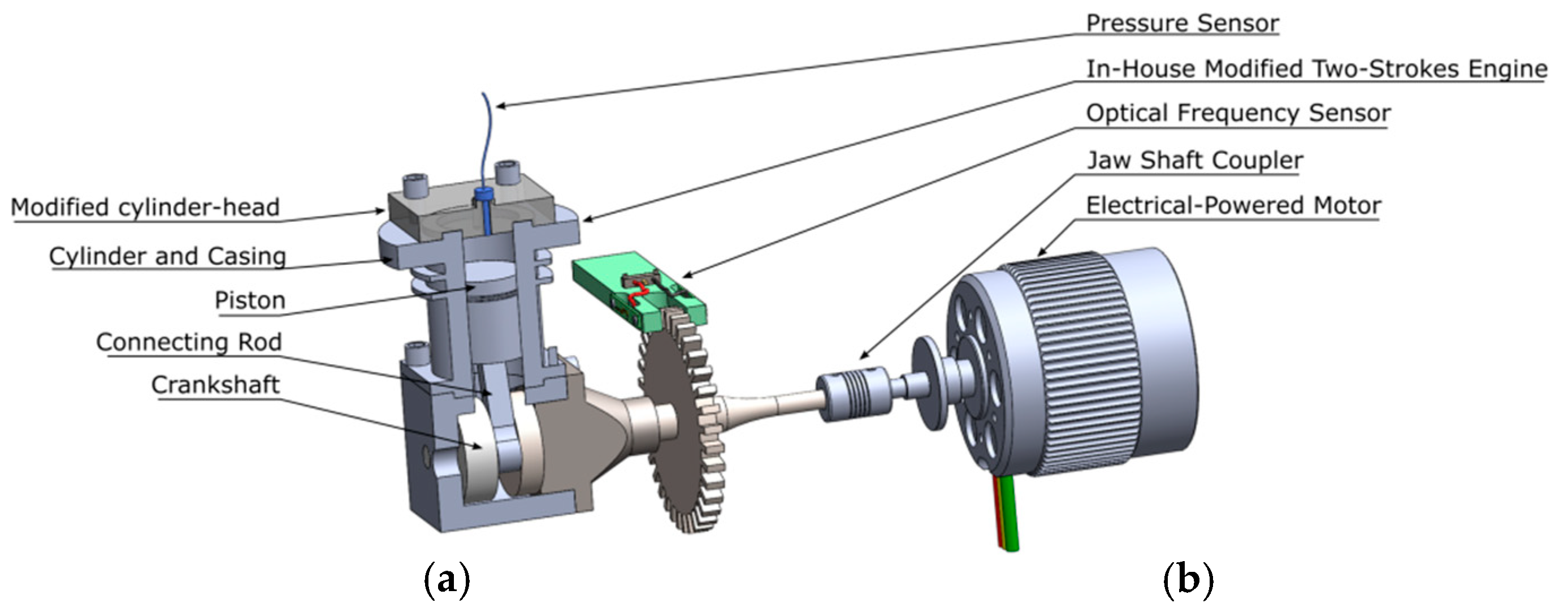
The work presented here is applied to an in-house-modified two-stroke piston-based synthetic jet. Figure 2 shows the two main components of the actuator: (1) The electric motor, and (b) the four-stroke engine. The velocity of the electric motor is variable and can be adjusted by the supply current. With a small jaw shaft coupler, the electric motor is connected to the crankshaft axis.
The cylinder of the two-stroke engine is modified so that the inlet and the exhaust ports are obstructed. The cylinder head is then replaced by a flat plate featuring a cylindrical exit nozzle at its center (d = 2.7 mm). In Figure 2 the open piston engine without the modified cylinder head is shown. The piston has a displacement of 4.89 cc.
The combination of the displacement and the small size of the outlet enabled to create a synthetic jet at the exit nozzle. A setscrew in the modified cylinder head allows the installation of a Kulite sensor that could capture the time-resolved chamber pressure. Figure 3 shows the head of the piston with the outlet and the attached pressure probe next to it.
On the axis of the electric motor and the stroke engine, a disk with 60 gaps is installed. A sensor can sense the gaps and convert the data into the rotational speed. In this study the piston stroke is set at 3 driving frequencies—5030 rpm (83 Hz), 7000 rpm (117 Hz), and 9977 rpm (167 Hz).
The piston cycle can be decomposed into two parts: Firstly, the piston compresses the air in the chamber and produces a hot and high speed air jet through the circular orifice, thereby increasing the pressure and temperature of the chamber. In the second half of the cycle, the piston expands the air in the chamber, reducing its pressure and temperature, and the orifice sucks in the surrounding ambient air.
2.1.2. Hot- and Cold-Wire Anemometry
The hot- and cold-wire are manipulated by means of a high precision mechanical robotic arm. For the hot- and cold-wire measurement a probe of type 55P71 from Dantec Dynamics (Copenhagen, Denmark) is used. The probe is a parallel array hot-wire probe that is usually operated in the CT (Constant Temperaure) mode, but is used in this study by taking one wire for the HWA, while measuring the temperature with the second wire in CC (Constant Current) mode. A Dantec Streamware A/D Conditioner is then used for the acquisition. Six hundred samples are taken, at a 10 kHz frequency rate, for each measuring point. The properties of the wire used are provided in Table 1.
The wires disturb the flow and have an influence on measurements behind the disturbance. Using the wires in a parallel configuration has the advantage to minimize the interaction between the wires, compared to e.g., a classical X-array hot-wire probe. The hot- and cold-wire are very sensitive to calibration shifts. Therefore, the calibration of both techniques has to be done on the same day as the measurement.
2.1.3. Unsteady Cavity Pressure Transducer
An unsteady piezoresistive pressure transducer Kulite© (XTL 190M) was placed on the upper side of the piston chamber, whose frequency and range of measurement are large enough to capture the compression-decompression cycle. In this study, 5000 points are acquired at 10 kHz rate. The sensor is first calibrated in the metrological laboratory of ONERA Lille, using a Mensor pressure controller of type CPC6000. The sum of the uncertainty of the sensor and the residual for the smallest pressure point corresponds to a deviation of less than 1% of the minimal pressure (35 kPa), while the uncertainty of the pressure value for in the highest pressure point corresponds to less than 0.4% of the maximum value (195 kPa).
2.1.4. Ambiant Pressure Transducer
Besides the Kulite sensor, a second pressure probe is used to sense the ambient pressure condition during the measurement. The ambient pressure is important for two reasons. On the one hand, the ambient condition in the test facility depends on the weather condition on the day of the measurement and has an influence on the experiments. On the other hand, in a free-jet, the static pressure is equal to the ambient pressure and thus, this measurement allows us to evaluate the results. For the ambient pressure measurement, a resonant pressure transducer (RPT) is used. The sensor is of type RPT 410 V from Druck Inc. (New York, NY, USA) with the accuracy ±0.5 mbar. The sensor has a pressure range of 60,000 Pa to 110,000 Pa, which is totally sufficient to measure the ambient pressure in the test facility. The accuracy for this sensor for temperatures between −10 °C and 50 °C is named to be ±50 Pa.
2.1.5. Laser Doppler Anemometry
The LDA measurements are realized, thanks to a Dantec back-scatter LDA System (FlowExplorer), including the optical probes and the signal processor. The optical probe is used for the laser beams generation and the intensity measurement of the scattered light. The signal processor (BSA) converts the signal from the optical probes into velocity. A lens with a focal length of 300 mm is used, which results in an angle of 11.31° between the beams and allows for the measurement of velocities ranging up to 300 m/s. Further than this value, the Signal-to-Noise Ratio is too low to obtain an accurate measurement. The used lens generates a probe volume length of 0.7 mm, which means it can measure the particles in the jet without the influence of particles around the jet. For the LDA measurements, the air is seeded with oil particles of size about 100 μm. For each measurement points, expected number of bins is acquired to reach a validation rate close to 100%. The optical probe of the FlowExplorer is installed with a vertical angle of 6°. Therefore, one of the beams is almost parallel to the surface of the jet outlet, while the other beam points in the outlet. With this setup it becomes possible to measure at a height of x = 1 mm above the outlet. Trying to set the probe volume closer to the outlet is not successful and leads to strong reflections of the beams on the object, which makes the measurement unfeasible, as shown in Figure 4.
2.1.6. Schlieren Photography
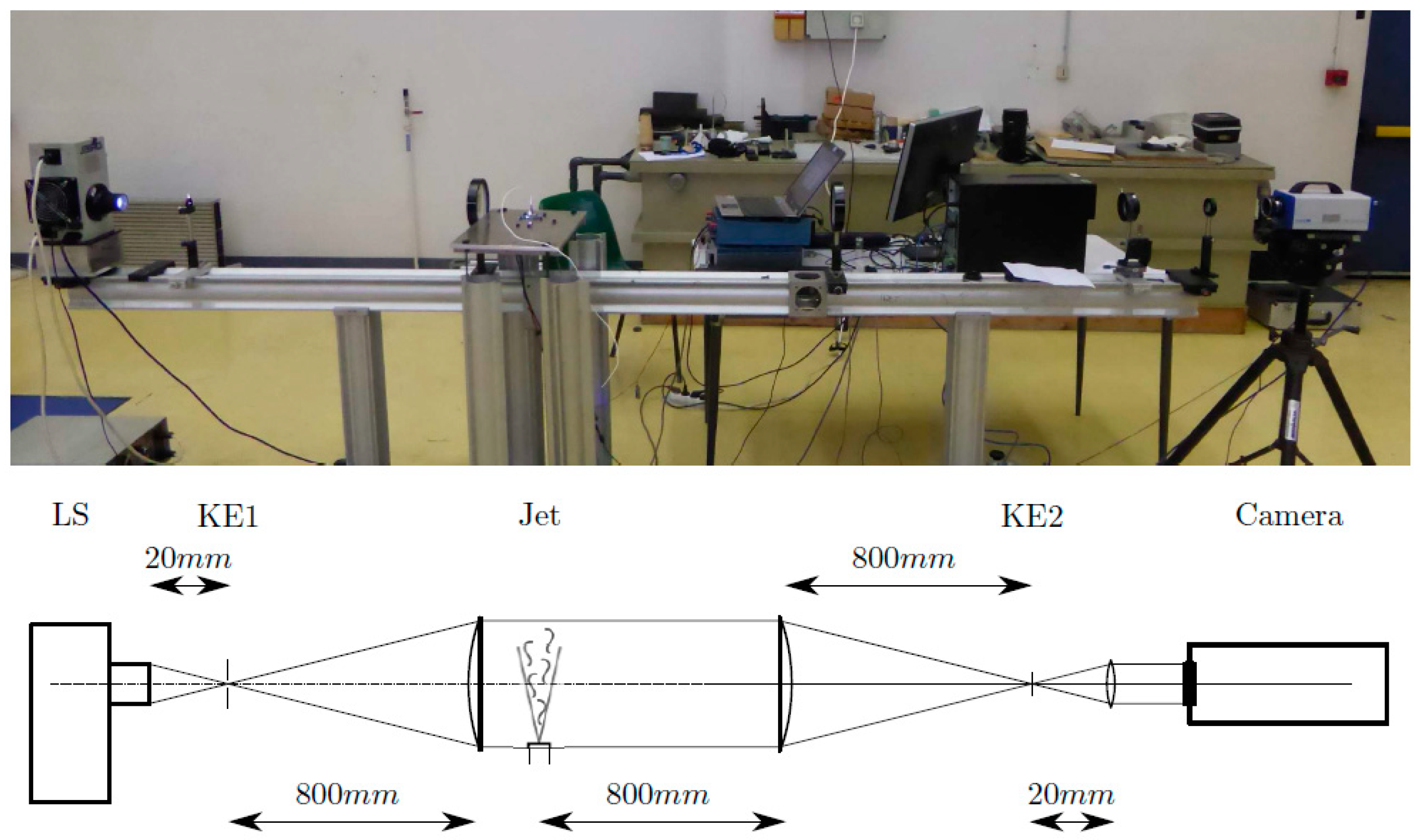
For the Schlieren Photography, the chosen camera is a Cam-Recorder 450 provided by Optronics (Goleta, CA, USA) and has a frame rate of up to 1000 fps, which allows enough resolution of the flow despite the synthetic jet’s high frequency. Figure 5 shows a picture of the setup, as well as the schematic drawing of the lens system. On the left side is the lamp that is used as the source of non-coherent white xenon light (LS). The lens system in the lamp housing (ORIEL 66055) has a focal length of f1 = 20 mm. A circular knife edge (KE1) is placed in the focus of the light source to decrease the blur in the image, by cutting off light rays that are not in the focus. A lens (L1) with a diameter of 120 mm and a focal length of fL1 = 800 mm collimates the light rays and a second lens (L2), with the same diameter and focal length, brings the light rays to a focus again. In the regime in between the two lenses, L1 and L2, the light rays are parallel, and the observed object has to be placed 800 mm (focal length of L2) in front of the second lens. A second knife edge (KE2) is placed in the focus again to cut off parts of the light. A third lens (L3), with a diameter of 30 mm, is placed in front of the camera to collimate the light rays again and refocus the light rays to increase the sharpness of the image.
2.1.7. Shadowgraphy
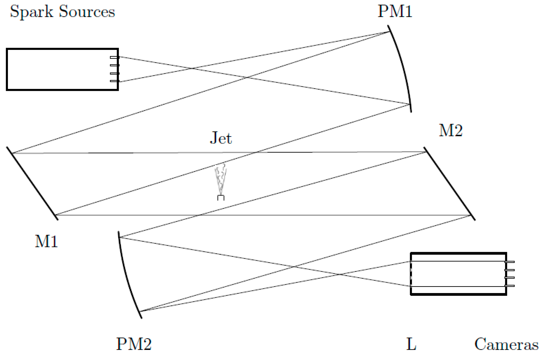
Another setup used with the optical methods, is the Z-type shadowgraphy system. In contrast to the previous lens-type system, parabolic mirrors are used instead of lenses for this configuration. Therefore, the spherical aberration of the lenses does not occur. The schematic drawing of the used system in Figure 6 is a slightly modified Z-type system, since two additional plane mirrors are used, M1 and M2. The parabolic mirrors PM1 and PM2 replace the lenses of the previous setup. To change the shadowgraphy to the Schlieren method, knife edges have to be placed in the focal length of PM2 in Figure 6. In the front plane of the camera box, a system of lenses (L) is installed to focus the light rays on the cameras. The 12 Cranz-Schardin spark sources, together with 12 cameras, create a system that works as a slow-motion camera. The sparks of the sources are generated with a time shift, which makes it possible to take the 12 images with a frequency of up to 5 MHz. For a frequency of the synthetic jet of 150 Hz (9000 rpm), the time lapse between the sparks is set to 280 μs. This value results from dividing the period of the jet and dividing it by the amount of sparks. This means that the time between two images, taken by the cameras, is 560 μs.
2.2. Methods
As stated in the introduction, classical approaches for indirect measurement must be tailored to take into account compressibility effects. Since LDA is a direct method that is still valid in the subsonic regime, and Schlieren and Shadowgraphy are qualitative methods that are based on compressibility effects, there will be a need to use a tailored approach with the wired anemometry technique. This section is therefore devoted to explaining the hot- and cold-wire method, its calibration, sensitivity and the way to obtain the temperature, mass flow and velocity from the raw electrical signals.
The main idea is to register data from the cold-wire and simultaneously from the hot-wire. The temperature can be recovered from the cold wire signal, and the mass flux and speed from the hot-wire signal, with aid of the temperature data. For further discussions and details on the calibration range and technique limitations, the reader can refer to Reference [23].
2.2.1. Calibration Equation for Hot Wire
Based on the studies of King [26], the Nusselt number , which is the ratio of convective to conductive heat transfer that characterizes the heat exchange of the hot-wire and the fluid can be related to the fluid’s Reynolds number , the ratio of inertial forces to viscous forces, as
where and are constants and a value of n = 0.5 suggested by King leads to the so called King’s law.
Neglecting diffusion and radiation, and assuming that the Joule heating is the key driver of heat exchange, the Nusselt number relates to the electric voltage as
where is the electrical resistance of the wire, is its length, is the thermal conductivity of the fluid, and are the temperature of the wire and the fluid respectively. These are approximately constant properties, implying that follows a linear regression with the Nusselt number.
The dependency between the electric voltage E and the Reynolds number is obtained by using King’s law as Ansatz and combining the constant properties in two new parameters and , functions of the temperature of the fluid:
A first order Taylor expansion in temperature leaves the correlation which is used in this study:
where is the velocity, the density and A and B are constants to be experimentally determined.
2.2.2. Sensitivity
There are two common ways to express the sensitivities of the hot-wire. Morkovin [27] describes the fluctuation in the output voltage E’ in supersonic flow as
where is the total temperature , and are the sensitivity coefficients. To obtain this equation the properties are separated in time mean values and fluctuation terms: , ,.
Bruun [28] suggests to express the sensitivities for the fluctuation in the output voltage as
Since, following King’s law, the hot-wire output in compressible flow is sensitive to the mass flux.
Taking the time-average of the previous equation results, and assuming constant sensitivities, we obtain the following relation:
The value for these sensitivities can be found by placing the hot-wire in a flow and individually varying the mass flux and the stagnation temperature, while measuring the response of the output voltage. Therefore, special equipment is necessary to ensure the conditions for the measurement.
2.2.3. Velocity Decoupling
So far, only results for the mass flux and recovery temperature, and not for the velocity, are obtained. To find the density of the flow, using the ideal gas law, the static flow temperature is missing. Since the velocity is unknown as well, it is not possible to get the static temperature T just from the definition of the recovery temperature ,
where is the freestream temperature, r is the recovery factor, the freestream velocity and the constant heat capacity.
Olczyk [7] suggests an iterative method to calculate the density of the flow. The mass flux and the recovery temperature are measured with the wires. Since the stream of the synthetic jet is a free-jet, which flows in the environment, the static pressure of the flow is equal to the ambient pressure . In the first iteration step the static temperature of the flow is said to be equal to the recovery temperature . Using the ideal gas equation, the density of the first iteration can be calculated, which makes it possible to split the measured mass flux up and obtain the velocity . Since a constant Prandtl number and are assumed, the recovery factor can be calculated as Kurganov [29] suggests, for turbulent flows, and thus the temperature for the next iteration as well from its definition. Repeating the iteration leads to a convergence of the density. The stop criterion for this iterative procedure has been set as that the change in the density between two iterations is of the order of the machine epsilon.
3. Results and Discussion
3.1. Cavity Pressure
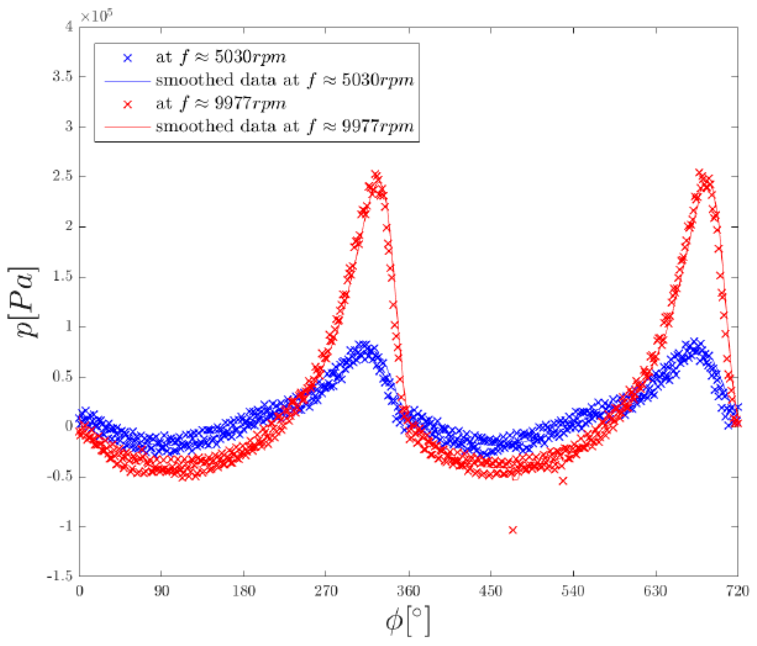
Figure 7 shows the data points of the relative cavity pressure at two different piston frequencies, 9977 and 5030 rpm. In this figure, the exhaust and intake regimes can be identified. The positive relative pressures correspond to the exhaust, which is generated by the compression of the air in the cavity, while the negative gauge pressure results from the expansion in the cavity and generates the intake flow. Due to the reason that the ambient pressure is constant during a measurement sequence, the cycles of the relative pressures are the same as for the absolute pressures, but with an offset in the ambient pressure.
The figure shows a clear asymmetry between the compression and decompression cycle. Another interesting feature is the singularity at 360°, in which the trend of the pressure drop suddenly changes from a linear to a much slower parabolic one. This kind of qualitative abrupt changes is, in fluid mechanics, commonly due to a bifurcation of a meaningful magnitude beyond a critical value. In this case, it is concluded through later evaluations that the change is due to the inflow Mach number trespassing the sonic threshold.
3.2. Temperature at Output
From the tension data of the cold-wire taken at the orifice exit it is possible to obtain the recovery temperature values, shown in Figure 8. The low temperatures correspond to the intake of air in the cavity, while the high temperatures occur during the exhaust of air. This fact is verified by synchronizing the temperature and the pressure measurements. In the cycle of the piston actuator, the piston motor compresses the air inside the cavity which increases the static temperature of the air.
Comparing the recovery temperature of the two settings at 5030 rpm and 9977 rpm, it turns out that the minima are within the same range for both settings, while the maxima for the higher frequency are considerably higher. The values are compared later in this section for different frequencies, to show the development of the maximal and minimal temperature better.
3.3. Mass Flux Output
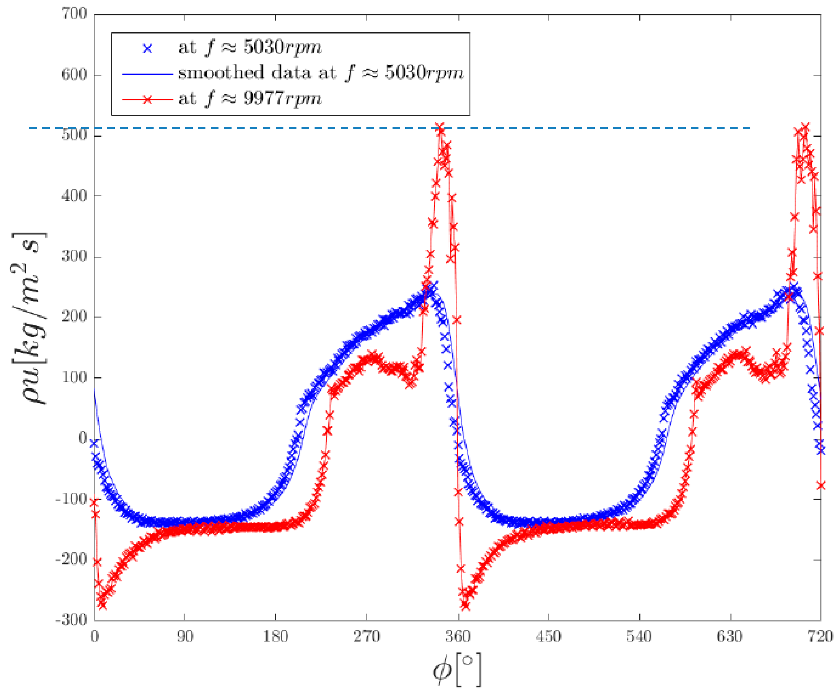
The recovery temperature in the flow is already obtained and the direction of the flow is defined by using the pressure data. Therefore, Equation (4) can be used to get the mass flux from the HWA tension data acquired at the orifice exit. The mass flux cycle is shown in Figure 9 for two complete cycles and the same frequencies as in previous diagrams. Positive sign means ejecting gas, while negative sign implies aspiration.
There are three main flow features arising from an inspection of the figure. The first one is the constant mass flow during the whole aspiration phase. Later it will be found that the regime is exactly sonic, suggesting the existence of a critical mass flow as it exists for the similar case of a reservoir-nozzle system [30]. The second is the mass flux varies in a slower rate during the onset of the jet phase than during its offset, when it falls sharply, for both chosen frequencies. Finally, the third features is the behavior of the mass flow at higher frequencies during the jet phase, and its transition to the aspiration phase, presents respectively dispersed-data at stagnated growth, and a steep over and undershoot. The latter features are suspected to be either artificial or inaccurate, as the following discussion suggests.
The aforementioned fast change short before transitioning to the aspiration phase is registered in the hot-wire signal. According to the evaluated data, the flow reaches supersonic velocities at these samples. In supersonic flow, Kovasznay [3] mentions that the relation between the heat transfer of a hot-wire in supersonic flow and the mass flux changes and thus, its equation has to be adjusted. However, this is only possible by performing a calibration in supersonic flow. This implies that this overshoot is no longer an accurate prediction of the true mass flow, since only calibrations in the subsonic domain have been made.
A steep decrease in the mass flux down to negative velocities, right after the maximal mass flux is reached, is also noticed. Furthermore, it can be observed a remarkably low minimum mass flux at 9977 rpm, before the values stabilized as the aspiration regime onsets. This effect only occurs for higher frequencies, larger than about 7000 rpm and gets stronger as the piston frequency increases. The need for the shadowgraphy visualization is, therefore, justified and the real change in temperature is very fast during the drop, as opposed as the measured one. The reason behind is that the ambient air fills rapidly the space which was previously covered by an over 200 °C air, temperature measured by the cold-wire. This fast change is not recorded by the cold-wire, which cannot follow a change of 200 °C to 20 °C in less than 560 μs, the span between two shadowgraphy measurements. This implies that the low minimum shown at Figure 9 is an artificial feature appearing because the cold-wire’s sampling capability is not fast enough to adapt and follow the rapidly changing unsteady temperature.
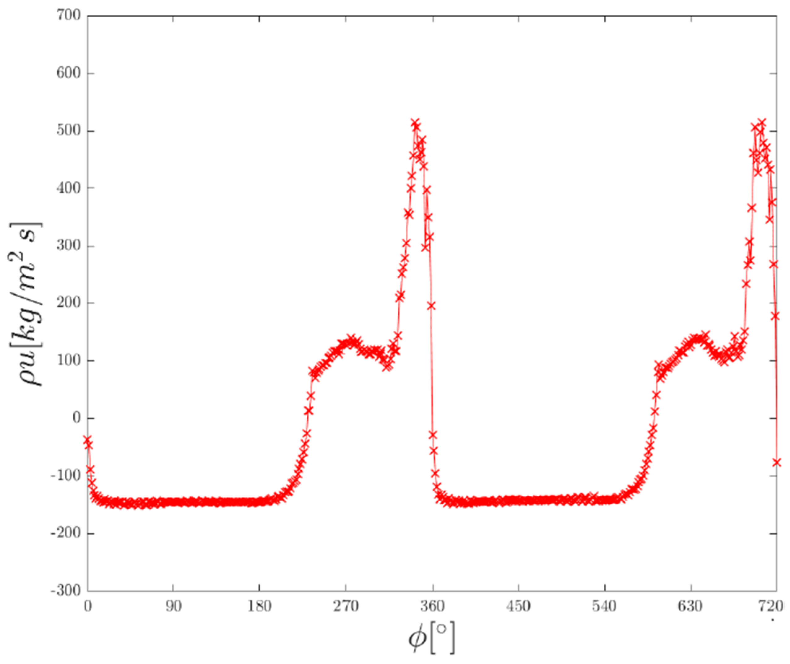
There is other evidence which supports this thesis: The effect does not appear in the voltage data of neither the hot-wire, nor of the cold-wire, and since the actuator is a zero-net mass flux actuator, the overall mass flux during one cycle has to be zero, and it is not in the case.
As a matter of fact, if following the shadowgraphy visualizations we introduced a hypothetical fast decay in temperature into the measurement as in Figure 10, the resulting mass flow chart would be the one shown in Figure 11, which contains no undershoot. To obtain this hypothetical behavior of a cold-wire with faster response, the cold-wire temperatures have to be adjusted to a behavior that is expected to occur for a faster sensor response. In the data in Figure 10 the decrease in the temperature is made steeper. The point in which the steep decrease starts is the same point as in the hot-wire data, so that the behavior of the cold-wire data corresponds to the hot-wire one. Then, Evaluating the tension data of the hot-wire now, using the manipulated recovery temperature, leads to the Figure 11 behavior.
3.4. Velocity Output
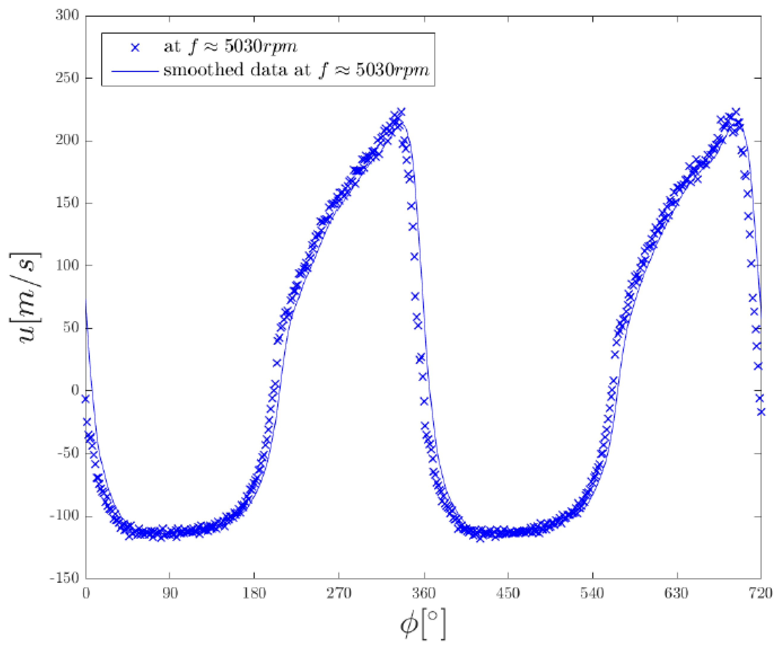
The velocity profile for the subsonic case is readily obtainable by means of Olczyk’s iterative procedure [7], based on the previously obtained temperature and mass flux data. The iterations converge for all frequencies smaller than 6500 rpm. LDA and Schlieren measurements, see Figure 15, show that the divergence is due to the reach of the supersonic regime, consistent with the fact that Olczyk’s procedure only works for subsonic flows.
Figure 12 shows the resulting velocity cycle at the orifice, which follows a similar evolution to that of the mass flux. As in the mass flux chart, the velocity stagnates during the inflow phase, it increases during the outflow phase, and then suddenly drops when transitioning to the inflow phase.
While the data shown in Figure 12 is taken at the orifice, the measurement can be very sensitive to the location of the probe. Figure 13 shows the recorded maximum and minimum velocity for different probe locations along the axis of the orifice. The chart’s x-coordinate begins at the orifice and is positive towards the outside (see axis definition in Figure 1).
The figure shows that while the maximum outwards velocity is constant in a neighborhood of the orifice, the maximum inwards velocity decays very fast with the distance. This implies that it exists a high sensitivity of the measurement on the spatial placement of the probe during the aspiration phase of a synthetic jet, and thus specifying the exact location of the measurement matters.
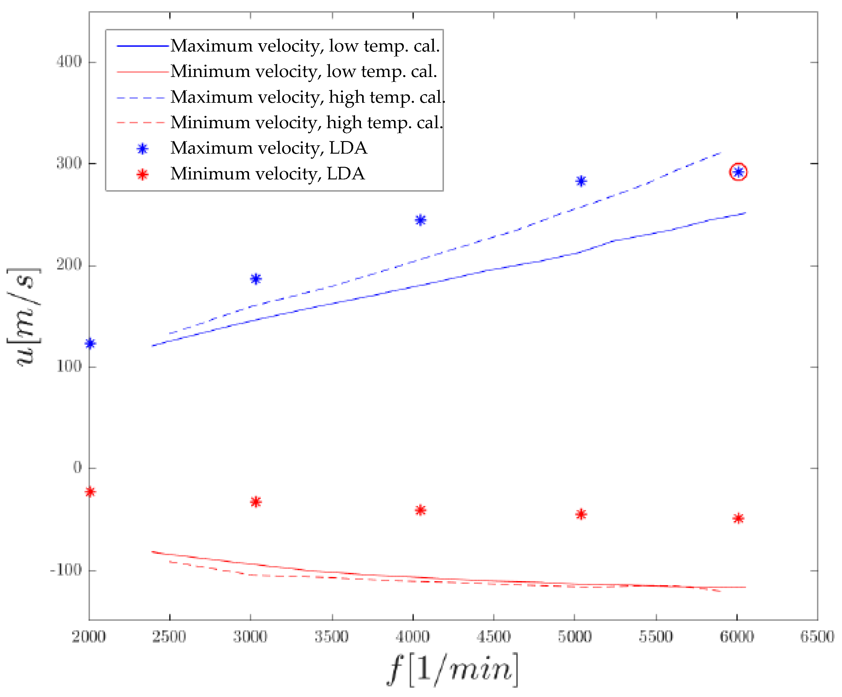
The maximal and minimal velocity peaks for different frequencies were measured at the orifice using the combined cold-wire/hot-wire technique, for different temperature calibrations, and at a 1mm distance with the LDA. The comparison is shown in Figure 14.
The blue data in Figure 14 represent maximum outwards velocity, and the red data represent maximum velocity towards the cavity. The dots represent LDA measurements, and the lines represent the hot-wire and cold-wire measurements. As the hot- and cold-wire measurements are concerned, the continuous line represents the output from a temperature calibration which did not cover the high temperature range, and the segmented line represents the output from a temperature calibration which did include up to 200 °C temperature values.
It is to be noted that the LDA measurement takes place at a distance of 1 mm outwards from the orifice, and the hot-wire/cold-wire measurements inside orifice. This explains the difference in value for the minimum speed.
The last LDA point, marked with a red circle, seems to not follow the trend. At this point, the excess of noise, due to the limited velocity range of the LDA lens (up to 300 m/s) could have influenced the measured velocity.
Comparing the hot- and cold-wire method with the LDA for the inwards velocities is challenging, for both measurements were taken at a distance of 1 mm and the velocity field is very sensitive at its surrounding during the intake. However, the LDA data is consistent with the previously presented spatial decay at a distance of 1 mm, see Figure 13, characterized by the hot- and cold-wire method. One should also notice that at the orifice exit, the inward velocity comes from the y-z plane direction, and that the hot- and cold-wire senses mostly x-component velocity.
It is shown earlier that the maximal velocity is not sensitive to the distance to the orifice where the measurement takes place. Therefore, the fact that the LDA measurement was taken at 1 mm distance of where the hot- and cold-wire measurements were taken should not affect the comparison. The second set of hot-wire and cold-wire measurements give a closer result to that of the LDA, resulting in a difference of about 10%, or 10 to 20 m/s.
The values for the minimum velocities of both hot-wire and cold-wire datasets seem identical, but diverge for the maximum velocities as they increase. This is consistent with the fact that both measurements involved different temperature calibrations, one only using ambient and colder temperature and the other ambient and hotter temperature. As the maximum velocity increases, the output temperature increases as well, and thus the dataset diverge.
It can be concluded, from the previous ideas, that the two measurement methods can give reliable results in the subsonic compressible regime, provided that the instruments do not exceed their measurement ranges and the hot- and cold-wire are properly calibrated, for both temperature and speed. However, it has been proven for this test case that even if they are not calibrated in the proper temperature range, the results can be satisfactory up to a 10% error.
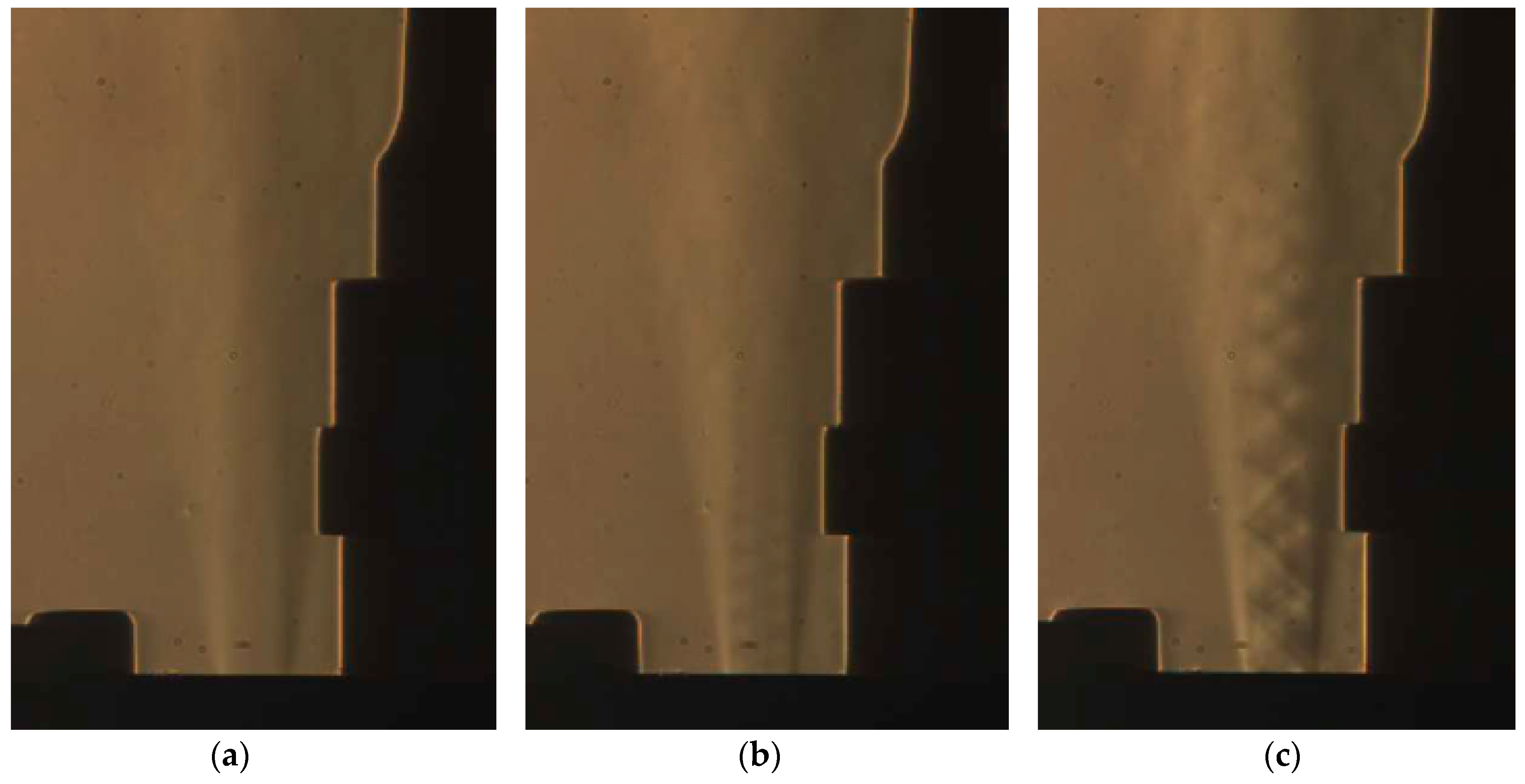
3.5. Visualization Schlieren
The qualitative Schlieren visualization helps determine the different regimes and qualitative flow characteristics, which have three main applications: Firstly, to understand the dynamics of the experiment and ensure that the setup has no leakages and has been properly made. Secondly, to conveniently choose the measurement instruments and the location of the probes. And thirdly and most importantly, to synchronize in time the qualitative effects with the quantitative measurements in a post-processing phase to cross-validate them.
The images shown at Figure 15 correspond to the flow generated by a 5030 rpm piston frequency, 7000 rpm, and 9977 rpm. It is shown that the velocity measured by both the hot- and cold-wire method and the LDA are consistent with the respectively subsonic, transonic and supersonic regimes of the images.
This visualization sheds further evidence on the fact that the divergence of the Olczyk’s iteration to extract the velocity from the hot-wire and cold-wire measurements for frequencies above 6500 rpm is caused by the onset of supersonic flow.
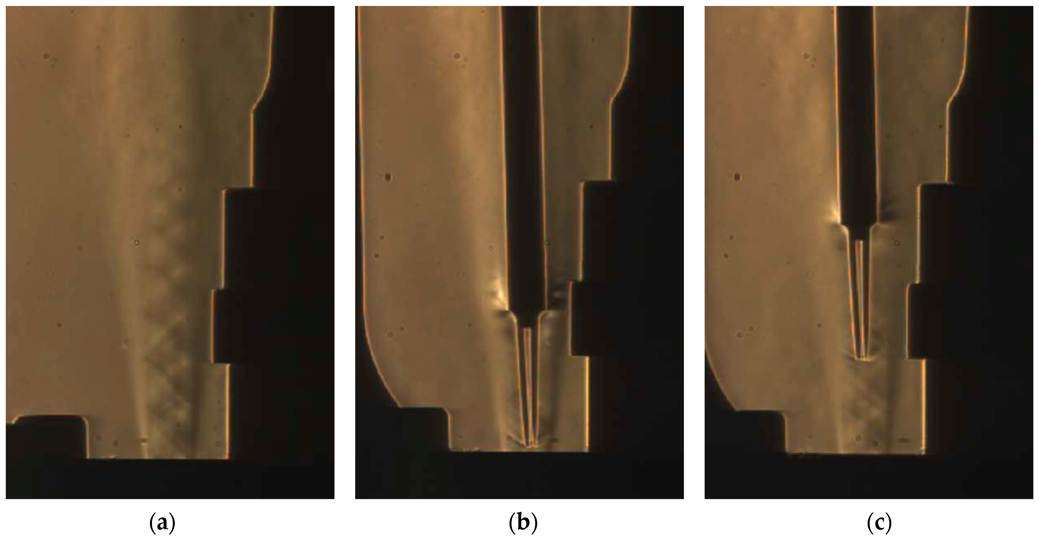
The set of images of Figure 16 was taken to demonstrate the influence and intrusiveness of the hot-wire technique. The parallel setup for the wires was chosen to avoid the influence of the heating coming from the hot-wire on the cold-wire. For the qualitative image, it appears that the shock waves in the jet between the orifice exit and the probe prongs still keep their original patterns.
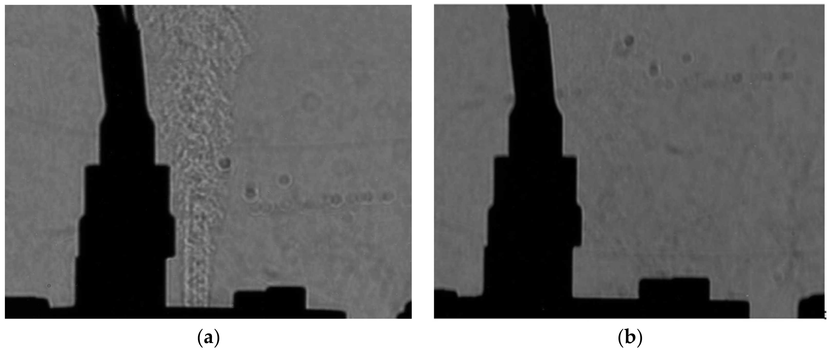
3.6. Visualization Shadowgraphy
In order to characterize the quick transition time between the exhausting phase and the intake phase, the images shown in Figure 17, made with the Cranz-Schardin spark sources and the shadowgraphy method, are analyzed.
The flow oscillates at 9000 rpm, or 150 Hz. The right picture follows the picture on the left with a time gap of 560 μs, or 8% of the complete piston period. In the left image the supersonic flow with the expansion fans and the compression shocks appears. 560 μs later, in the right picture, the jet structure disappears completely. This means that, at this frequency, the change in temperature with time is about 3 × 10⁵ K/s between the two phases, this explains why the cold-wire could not capture the transition.
4. Conclusions and Future Work
A benchmark of different measurement techniques has been carried out, and the dynamic response of a piston-based synthetic jet actuator working in compressible regime has been characterized. Indirect methods such as the cold- and hot-wire anemometry have been adapted and combined to recover the velocity, and different time-resolved data such as the cavity pressure, as well as the velocity, temperature and mass flow at the synthetic jet output have been compared from different measurement instruments.
As the combined cold-wire and hot-wire technique to measure temperature and speed is concerned, a study on the sensitivity of the velocity with respect to the temperature calibration has also been made. The experiment has been carried out with two different calibrations for the cold-wire: One with low temperatures and thus extrapolation, and another one with high temperatures and interpolation. The velocity measurements from the proper high temperature calibration show the best fit with the LDA results, as they differ 10% at most. The deviation with respect to the results from the cold temperature calibration increases as the piston frequency, and thus the output temperature, increases.
A strong velocity gradient has been measured in the neighborhood of the orifice during the aspiration phase, so an accurate measurement of the position of the probe is necessary for the repeatability of the results. This accurate positioning was possible thanks to an automatized workbench.
LDA results show consistency with the cold-wire and hot-wire technique during the exhausting phase. During the aspiration phase, a direct comparison was not possible, due to the fact that reflections of the laser on the synthetic jet top orifice were unavoidable, unless the laser beam was placed at least at a distance from the orifice of 1 mm. However, the fast decay of velocity with the distance to the synthetic jet orifice was characterized, and the values measured by the LDA at a distance of 1 mm are consistent with this characterization.
A strong density time-derivative, and thus temperature time-derivative, has been measured in the vicinity of the orifice in the transition between the exhausting and the aspiration phase. The change of temperature in time has been estimated to 200 K per 560 μs, estimation in excess as the shadowgraphy did not allow further resolution on time. The cold-wire could not capture this fast transition, and this implies that the recorded mass-flow during a short period after that drop in temperature was not accurate.
The measurement of the velocity was possible for the compressible subsonic flows. However, when using higher piston frequencies, the velocity iterations diverged, and Schlieren measurements showed that the reason behind was a change in the flow regime from subsonic to supersonic. More research is needed to apply the cold-wire and hot-wire technique to the transonic regime.
Author Contributions
Conceptualization, P.M., J.D. and Q.G.; Methodology, P.F., P.M., C.O., J.D. and Q.G.; Software, J.D.; Formal Analysis, P.M.; Writing-Original Draft Preparation, P.F. and C.O.; Writing-Review & Editing, Q.G.; Supervision, Q.G.
Funding
Part of this work has been financed by the ELSAT2020 project, co-financed by the European Union with the European Regional Development Fund, the French state and the Hauts-de-France Region Council.
Conflicts of Interest
The authors declare no conflict of interest.
References
- Kupferschmied, P.; Köppel, P.; Gizzi, W.; Roduner, C.; Gyarmathy, G. Time-resolved flow measurements with fast-response aerodynamic probes in turbomachines. Meas. Sci. Technol. 2000, 11, 1036–1054. [Google Scholar] [CrossRef]
- Blackwelder, R.F. Hot-Wire and Hot-Film Anemometers. In Methods of Experimental Physics; Emrich, R.J., Ed.; Academic Press, Inc.: New York, NY, USA, 1981. [Google Scholar]
- Kovasznay, L.S.G. The Hot-Wire Anemometer in Supersonic Flow. J. Aeronaut. Sci. 1950, 17, 565–572. [Google Scholar] [CrossRef]
- Lomas, C.G. Fundamentals of Hot-Wire Anemometry; Cambridge University Press: Cambridge, UK, 2011. [Google Scholar]
- Horstman, C.C.; Rose, W.C. Hot-Wire Anemometry in Transonic Flow; NASA: Washington, DC, USA, 1975.
- Smits, A.J.; Muck, K.C. Constant temperature hot-wire anemometer practice in supersonic flows. Exp. Fluids 1984, 2, 33–41. [Google Scholar] [CrossRef]
- Olczyk, A. Problems of unsteady temperature measurements in a pulsating flow of gas. Meas. Sci. Technol. 2008, 19, 055402. [Google Scholar] [CrossRef]
- Zong, H.; Kotsonis, M. Formation, evolution and scaling of plasma synthetic jets. J. Fluid Mech. 2018, 837, 147–181. [Google Scholar] [CrossRef]
- Antonia, R.A.; Browne, L.W.B.; Chambers, A.J. Determination of times constants of cold-wires. Rev. Sci. Instrum. 1981, 52, 1382–1385. [Google Scholar] [CrossRef]
- Buttsworth, D.R.; Jones, T.V. A fast-response total temperature probe for unsteady compressible flows. J. Eng. Gas Turbines Power 1998, 120, 694–702. [Google Scholar] [CrossRef]
- Johnston, R.; Fleeter, S. Compressible flow hot-wire calibration. Exp. Fluids 1997, 22, 444–446. [Google Scholar] [CrossRef]
- Cukurel, B.; Acarer, S.; Arts, T. A novel perspective to high-speed cross-hot-wire calibration. Exp. Fluids 2012, 53, 1073–1085. [Google Scholar] [CrossRef]
- Johnson, D.A. Laser Doppler Anemometry; NASA: Washington, DC, USA, 1988.
- Settles, G.S.; Hargather, M.J. A review of recent developments in schlieren and shadowgraph techniques. Meas. Sci. Technol. 2017, 28, 042001. [Google Scholar] [CrossRef]
- Dandois, J.; Garnier, E.; Sagaut, P. DNS/LES of Active Separation Control. In Direct and Large-Eddy Simulation, 6th ed.; Lamballais, E., Friedrich, R., Geurts, B.J., Métais, O., Eds.; Springer: Dordrecht, The Netherlands, 2016; pp. 459–466. [Google Scholar]
- Cattafesta, L.N. Actuators for Active Flow Control. Annu. Rev. Fluid Mech. 2011, 43, 247–272. [Google Scholar] [CrossRef]
- Gao, S.; Zhang, J.Z.; Tan, X.M. Experimental study on heat transfer characteristics of synthetic jet driven by piston actuator. Sci. China Technol. Sci. 2012, 55, 1732–1738. [Google Scholar] [CrossRef]
- Lee, C.Y.Y.; Woyciekoski, M.L.; Copetti, J.B. Experimental study of synthetic jets with rectangular orifice for electronic cooling. Exp. Therm. Fluid Sci. 2016, 78, 242–248. [Google Scholar] [CrossRef]
- Van Buren, T.; Amitay, M. Comparison between finite-span steady and synthetic jets issued into a quiescent fluid. Exp. Therm. Fluid Sci. 2016, 75, 16–24. [Google Scholar] [CrossRef]
- Van Buren, T.; Whalen, E.; Amitay, M. Vortex formation of a finite-span synthetic jet: High Reynolds numbers. Phys. Fluids 2014, 26, 014101. [Google Scholar] [CrossRef]
- Paolillo, G.; Salvatore, C.; Cardone, G. The evolution of quadruple synthetic jets. Exp. Therm. Fluid Sci. 2017, 89, 259–275. [Google Scholar] [CrossRef]
- Smith, B.L.; Swift, G.W. A comparison between synthetic jets and continuous jets. Exp. Fluids 2003, 34, 467–472. [Google Scholar] [CrossRef]
- Maier, P. Experimental Characterization of an Unsteady Compressible Jet. Master’s Thesis, Institute of Aerodynamics and Gas Dynamics, the University of Stuttgart, Stuttgart, Germany, 2017. [Google Scholar]
- Gallas, Q.; Pruvost, M. Characterization of fluidic micro-actuators. In Proceedings of the Workshop on Safety and Control Valves, Von Karman Institute, Rhode-St-Genèse, Belgium, 8–9 April 2015. [Google Scholar]
- Ternoy, F.; Dandois, J.; Eglinger, E.; Delva, J. Overview of ONERA Fluidic Actuators in Aerodynamics. In Proceedings of the Actuator 2018, Bremen, Germany, 25–27 June 2018. [Google Scholar]
- King, L.V. On the Convection of Heat from Small Cylinders in a Stream of Fluid: Determination of the Convection of Small Platinum Wires with Applications to Hot-Wire Anemometry. Phil. Trans. R. Soc. Lond. A 1914, 90, 563–570. [Google Scholar]
- Morkovin, M.V. Fluctuations and Hot-Wire Anemometry in Compressible Flows; North Atlantic Treaty Organization: Paris, France, 1956; p. 24. [Google Scholar]
- Bruun, H.H. Hot-Wire Anemometry; Oxford University Press: Oxford, UK, 1995. [Google Scholar]
- Kurganov, V.A. Adiabatic wall temperature. Available online: http://www.thermopedia.com/content/291/ (accessed on 7 September 2018).
- Briassulis, G.; Honkan, A.; Andreopoulos, J.; Watkins, C.B. Applications of hot-wire anemometry in shock-tube flows. Exp. Fluids 1995, 19, 29–37. [Google Scholar] [CrossRef]
Figure 1.
Schematic of the measurement setup for the cold-wire, hot-wire and pressure sensors (a) hardware setup, (b) 3D view.
Figure 1.
Schematic of the measurement setup for the cold-wire, hot-wire and pressure sensors (a) hardware setup, (b) 3D view.

Figure 2.
Main components of the synthetic jet actuator: (a) Open piston motor, and (b) electric motor.
Figure 2.
Main components of the synthetic jet actuator: (a) Open piston motor, and (b) electric motor.

Figure 3.
Modified cylinder head with the nozzle of d = 2.7mm and the attached pressure probe.

Figure 4.
Cylinder head with the nozzle of d = 2.7mm and the attached pressure probe.

Figure 5.
Picture and schematic drawing of the lens-type Schlieren test setup.

Figure 6.
Schematic drawing of the Z-type shadowgraphy test setup with the spark system.

Figure 7.
Evolution of the relative cavity pressure over two cycles at the frequencies 5030 and 9977 rpm.
Figure 7.
Evolution of the relative cavity pressure over two cycles at the frequencies 5030 and 9977 rpm.

Figure 8.
Evolution of the recovery temperature over two cycles at the frequencies 5030 and 9977 rpm, taken at the orifice exit.
Figure 8.
Evolution of the recovery temperature over two cycles at the frequencies 5030 and 9977 rpm, taken at the orifice exit.

Figure 9.
Evolution of the mass flux over two cycles at the frequencies 5030 and 9977 rpm, taken at the orifice exit. The dotted horizontal line shows the limit of the calibration range.
Figure 9.
Evolution of the mass flux over two cycles at the frequencies 5030 and 9977 rpm, taken at the orifice exit. The dotted horizontal line shows the limit of the calibration range.

Figure 10.
Hypothetical evolution of the temperature over two cycles at the frequency 9977 rpm, taken at the orifice exit. A discontinuous temperature drop is introduced.
Figure 10.
Hypothetical evolution of the temperature over two cycles at the frequency 9977 rpm, taken at the orifice exit. A discontinuous temperature drop is introduced.

Figure 11.
Hypothetical evolution of the mass flow over two cycles at the frequency 9977 rpm, taken at the orifice exit, as a result of the temperature profile shown at Figure 10.
Figure 11.
Hypothetical evolution of the mass flow over two cycles at the frequency 9977 rpm, taken at the orifice exit, as a result of the temperature profile shown at Figure 10.

Figure 12.
Evolution of the velocity over two cycles at the frequency 5030 rpm, taken at the orifice exit.
Figure 12.
Evolution of the velocity over two cycles at the frequency 5030 rpm, taken at the orifice exit.

Figure 13.
Maximal inwards (crosses x) and outwards (asterisks *) velocity measured at the synthetic jet output, as a function of the outwards distance to the synthetic jet output, at the frequency 5030 rpm.
Figure 13.
Maximal inwards (crosses x) and outwards (asterisks *) velocity measured at the synthetic jet output, as a function of the outwards distance to the synthetic jet output, at the frequency 5030 rpm.

Figure 14.
Maximum outwards (blue) and inwards (red) velocity as a function of the piston frequency. Comparison of the Laser Doppler anemometry (LDA) measurements (dots) with the hot- and cold-wire measurements (lines). Sensitivity of the hot- and cold-wire velocity measurement on the cold-wire calibration: Results using only extrapolation and low temperature to calibrate (continuous line), and interpolation and the whole range of temperatures (segmented line).

Figure 15.
Schlieren images of the jet at the frequency (a) 5030 rpm, (b) 7000 rpm, and (c) 9977 rpm.
Figure 15.
Schlieren images of the jet at the frequency (a) 5030 rpm, (b) 7000 rpm, and (c) 9977 rpm.

Figure 16.
Intrusiveness of the hot- and cold-wire method on the flow (a) without the probe, (b) with probe above the orifice exit, (c) with probe away from orifice exit. Images taken with the Schlieren method and a piston frequency of 9977 rpm.
Figure 16.
Intrusiveness of the hot- and cold-wire method on the flow (a) without the probe, (b) with probe above the orifice exit, (c) with probe away from orifice exit. Images taken with the Schlieren method and a piston frequency of 9977 rpm.

Figure 17.
Shadowgraphy pictures of the flow separated by 560 μs during (a) expulsion phase and (b) ingestion phase of the synthetic jet.
Figure 17.
Shadowgraphy pictures of the flow separated by 560 μs during (a) expulsion phase and (b) ingestion phase of the synthetic jet.


Table 1.
Properties of the wire of type 55P71 used for the HWA.
| Sensor Material | Plated Tungsten |
|---|---|
| Sensor diameter | 5 μm |
| Sensor length | 1.25 mm |
| Sensor resistance at ϑref = 20 °C | 3.41 Ω |
| Sensor lead resistance | 0.5 Ω |
| Temperature coefficient at ϑref | 0.36%/°C |
© 2018 by the authors. Licensee MDPI, Basel, Switzerland. This article is an open access article distributed under the terms and conditions of the Creative Commons Attribution (CC BY) license (http://creativecommons.org/licenses/by/4.0/).
Share and Cite
MDPI and ACS Style
Fernandez, P.; Delva, J.; Ott, C.; Maier, P.; Gallas, Q. Experimental Measurement Benchmark for Compressible Fluidic Unsteady Jet. Actuators 2018, 7, 58. https://doi.org/10.3390/act7030058
AMA Style
Fernandez P, Delva J, Ott C, Maier P, Gallas Q. Experimental Measurement Benchmark for Compressible Fluidic Unsteady Jet. Actuators. 2018; 7(3):58. https://doi.org/10.3390/act7030058
Chicago/Turabian StyleFernandez, Pablo, Jerome Delva, Celestin Ott, Philipp Maier, and Quentin Gallas. 2018. "Experimental Measurement Benchmark for Compressible Fluidic Unsteady Jet" Actuators 7, no. 3: 58. https://doi.org/10.3390/act7030058
Note that from the first issue of 2016, this journal uses article numbers instead of page numbers. See further details here.