Article

High-Throughput Ground Cover Classification of Perennial Ryegrass (Lolium Perenne L.) for the Estimation of Persistence in Pasture Breeding

1
Agriculture Victoria, Hamilton Centre, Hamilton, Victoria 3300, Australia
2
School of Agriculture and Food, Faculty of Veterinary and Agricultural Sciences, the University of Melbourne, Victoria 3010, Australia
3
Agriculture Victoria, Ellinbank Centre, Ellinbank, Victoria 3821, Australia
4
Agriculture Victoria, AgriBio, Centre for AgriBioscience, Bundoora, Victoria 3083, Australia
5
School of Applied Systems Biology, La Trobe University, Bundoora, Victoria 3086, Australia
*
Author to whom correspondence should be addressed.
Agronomy 2020, 10(8), 1206; https://doi.org/10.3390/agronomy10081206
Submission received: 14 July 2020 / Revised: 3 August 2020 / Accepted: 14 August 2020 / Published: 17 August 2020

Abstract

:
Perennial ryegrass (Lolium perenne L.) is one of the most important forage grass species in temperate regions of Australia and New Zealand. However, it can have poor persistence due to a low tolerance to both abiotic and biotic stresses. A major challenge in measuring persistence in pasture breeding is that the assessment of pasture survival depends on ranking populations based on manual ground cover estimation. Ground cover measurements may include senescent and living tissues and can be measured as percentages or fractional units. The amount of senescent pasture present in a sward may indicate changes in plant growth, development, and resistance to abiotic and biotic stresses. The existing tools to estimate perennial ryegrass ground cover are not sensitive enough to discriminate senescent ryegrass from soil. This study aimed to develop a more precise sensor-based phenomic method to discriminate senescent pasture from soil. Ground-based RGB images, airborne multispectral images, ground-based hyperspectral data, and ground truth samples were taken from 54 perennial ryegrass plots three years after sowing. Software packages and machine learning scripts were used to develop a pipeline for high-throughput data extraction from sensor-based platforms. Estimates from the high-throughput pipeline were positively correlated with the ground truth data (p < 0.05). Based on the findings of this study, we conclude that the RGB-based high-throughput approach offers a precision tool to assess perennial ryegrass persistence in pasture breeding programs. Improvements in the spatial resolution of hyperspectral and multispectral techniques would then be used for persistence estimation in mixed swards and other monocultures.

1. Introduction

Perennial ryegrass (Lolium perenne L.) has become the most widely sown perennial forage grass in temperate regions due to its high productivity, nutritive value, and ability to tolerate a range of grazing practices. However, it may have poor persistence due to its low tolerance to both abiotic and biotic stresses [1]. Differences in persistence between perennial ryegrass cultivars may arise from variations in tolerance to abiotic and biotic stresses such as drought, heat, pests, and diseases. The productivity of a sward may depend on the number of plants per unit area and the size of individual plants [2]. The size of individual plants is influenced by the number of living tillers per plant and the size of the individual tillers. Tiller density of a sward can decline with time and gradually expose bare ground, which in turn provides opportunities for invading weed species to germinate and colonize. Tiller density decline will reduce the productivity of the sward in subsequent years.
The most profitable pasture relies on the process of a product (e.g., meat or milk) over time [3]. If the number of plants in a sward declines after being exposed to extreme stress conditions, the total financial benefits of the farm may decrease due to a reduction in pasture production and the subsequent costs associated with pasture renovation [4,5]. Moreover, if the expected dry matter production declines, additional purchased feed and/or a reduction in the stocking rate may be required to balance the energy requirements of livestock [6]. The additional expenses for supplementary feed, pasture renovation, and reducing the stocking rate are likely to negatively impact on financial returns for the farm system [7]. The improvement of persistence in pasture cultivars has become one of the primary objectives of breeding programs [2]. The assessment of persistence in pasture breeding depends on the visual estimation of ground cover or ranking populations (subjective measurement) by counting the number of surviving plants per unit area [1]. Taking data from manual methods at regular intervals may be satisfactory for ranking pasture cultivars in small-scale experiments composed of a smaller number of plots; however, more cost-effective tools are required for pasture persistence estimation in large-scale breeding programs. Senescent leaves, stems, and pseudostems in perennial ryegrass swards result from pasture senescence [8], which may be accompanied by chlorosis and the subsequent death of mature tissue. Pasture senescence is the process of the remobilization and transfer of soluble constituents from mature to immature plant tissues that occurs with the advancing age of plant parts, or through abiotic and biotic stresses [9]. Pasture senescence may indicate changes in plant growth, development, and resistance to abiotic and biotic stresses [10], and the amount of senescent pasture on the soil surface of breeding plots can be used as a key indicator of persistence in cultivar evaluation.
Due to rapid technology development, interest in exploring the use of high-throughput phenotyping (HTP) approaches has been reported for quantifying perennial ryegrass biomass, nutritive characteristics, and persistence in pasture breeding [11,12,13]. We have recently developed an object-based image analysis approach for perennial ryegrass persistence estimation [1]. The phenomic data derived from ground-based Red, Green, and Blue (RGB) color images and aerial-based multispectral images showed a positive correlation with the manually assessed pasture ground cover. However, the workflow was not sensitive enough to discriminate senescent pasture from bare ground in the breeding plots. Living healthy pasture absorbs most of the energy from incident radiation in the visible region and reflects a large portion of the energy in the 400–1100 nm wavelength region of the electromagnetic spectrum (EMS) [1]. The discrimination of green pasture from bare soil and senescent pasture is more likely using the spectral properties of reflectance spectrum in the 400–1100 nm wavelength region. However, the reflectance spectra of senescent pasture and bare ground lack the unique spectral signature in the 400–1100 nm wavelength region of the reflectance spectrum [14]. This makes the discrimination between soil and senescent pasture difficult or nearly impossible using the reflectance characters of the 400–1000 nm wavelength region. Therefore, the normalized difference senescent vegetation index (NDSVI) has been introduced to estimate the fractional senescent vegetation cover in grasslands using reflectance the spectra in the shortwave infrared (SWIR) region [15]. The NDSVI was computed by dividing the difference of the satellite-based shortwave infrared (1650 nm) and visible red (660 nm) bands by their summation. However, the spectral responses in these regions can be distorted due to the presence of moisture in senescent tissues. Cellulose, hemicellulose, lignin, and other structural components of plant tissue relate to wavelengths 2100 nm in the reflectance spectrum of senescent plant materials. The absorption near 2100 nm is absent from the soil or green vegetation reflectance spectra [16], and this can be used to discriminate the senescent fraction of pasture ground cover. Daughtry et al. [9] proposed the cellulose absorption index (CAI) to describe the presence of senescent plant-related absorption features in the 2000–2200 nm wavelength region. A recent study also showed that the CAI derived from satellite images has potential for the estimation of regional non-photosynthetic biomass in grassland [17]. Many other attempts have been made to estimate the senescent ground cover in grassland or conventional cropping using satellite-based remote sensed data [18,19,20]. The current ground level pixel resolution of a satellite is limited to 10–30 m2 per pixel, with an image update on average every 5–10 days [21]. Moreover, the spectral inconsistency of surface reflectance against solar and atmospheric cloud effects may reduce the quality of satellite-based phenomics data. Therefore, satellite imagery may not provide adequate image resolution and frequency for phenotyping pasture traits in breeding plots, and the adaption of satellite remote sensing remains challenging for pasture senescence estimation. The sensors deployed on unmanned aerial vehicles (UAV) and ground platforms such as unmanned ground vehicles (UGVs) and manual push-behind and motor-driven carts can achieve a ground sampling distance (GSD) as small as 2 cm [21]. The adaption of proximal sensing platforms may offer more precise and low-cost tools for pasture senescent estimation. Recent studies showed that proximal spectroradiometer and fluorescence sensors have been used in distinguishing non-photosynthetic plant materials from soils in laboratory conditions [22]. However, fluorescence imaging may not be an ideal technique for field-based phenotyping due to its high energy requirement to generate a fluorescence signal. Moreover, Cai et al. 2016 [23] showed that two time series of RGB images and an image processing algorithm can be used to quantify the progression of plant senescence in wheat and chickpea plants under a controlled environment. Therefore, high-resolution proximal RGB images and more precise algorithms such as machine leaning (ML) may offer the potential for pasture senescence estimation.
With improving computer power and advances in programming, the application of advanced machine learning (ML) algorithms has increased in remote sensing approaches for precision agriculture. The K-nearest neighbor (k-NN) analysis is a machine learning script and a decision making rule that can be used for investigating patterns of spatial distribution within two-dimensional datasets, such as RGB and multispectral images [24]. In the K-nearest neighbor analysis, images are classified according to the relationship of its k-NN with the reference data set (training or learning samples, manually labelled by an operator) [25]. The k-NN algorithm has been used in recent remote sensing studies for classifying agricultural land cover types using Landsat-5 TM imagery [26] and weed identification [27]. However, there is a lack of knowledge on the application of ML approaches in pasture phenotyping. This paper investigates advanced ML algorithms and the potential of vegetation indices to develop precise tools to estimate pasture senescence in breeding programs using high-throughput phenotyping.

2. Materials and Methods

2.1. The Study Site

The experiment was conducted at Lardner Park research facility in Lardner, Victoria, Australia (38.2156° S, 145.8746° E, 128 m above sea level; Figure 1). The study site consisted of a randomized complete block trial with 54 plots in three replicates. The size of a single plot was 5 m × 1.2 m, and the trial site covered approximately 400 m2. The trial was sown in autumn 2016 by Barenbrug Australia and managed with repeated cutting at approximately 5 cm height during the growing season. Harvests were scheduled to occur when the highest yielding plots were assessed to have approximately 2500 kg/ha biomass. The weed invasion of the trial was actively eliminated using mechanical methods and by spraying herbicide.

2.2. Visual Pasture Ground Fraction Estimation

Data collection was undertaken on 15 May 2019 at the autumn harvest three years after sowing. The ground cover (senescent and green fractions) was assessed after destructive harvest within a quadrat (50 cm × 50 cm) at three subsample points within each plot (red polygons in Figure 1) by three experienced researchers using a previously described protocol [28]. One hundred and sixty-two subsample data points were used for the visual ground fraction estimation. The visual ground fraction estimation was carried out within each subsample point after destructive harvesting using a shearing clipper (Model: VS84-S, Heiniger AG, Switzerland). The location of each subsample point was manually marked using luminous metal pegs to use the same location for subsequent data collection. The sample points were also located using a real-time kinematic global navigation satellite system (RTK GNSS) receiver (Model: Emlid Reach RS+, Emlid Ltd., Saint Petersburg, Russia) to identify the same location in the phenomic data extraction pipeline. The RTK GNSS receiver consisted of a base station and receiver, and was able to georectify at a 1 cm precision.

2.3. Dry Weight Ranking for Pasture Senescent Estimation

The dry weight ranking (DWR) technique was used as a manual method for ground cover classification [29]. A quadrat was placed at pre-defined sampling points of plots, and the standing biomass within the quadrat was cut at an approximately 5 cm height from the ground level using a shearing clipper (Model: VS84-S, Heiniger AG, Switzerland). Subsamples (200–300 g) were taken from each clipped sample and separated into three categories: living pasture, senescent pasture, and other (if anything is present). These fractions of each subsample were separately oven dried at 60 °C to a constant mass and weighed using a Mettler Toledo GmbH compact scale (Model: ICS6x5-1; Mettler-Toledo Ltd., Toledo, OH, USA) to the nearest 0.1 g. The percentage of the senescent pasture fraction was calculated using a method described in the standard DWR technique [29].

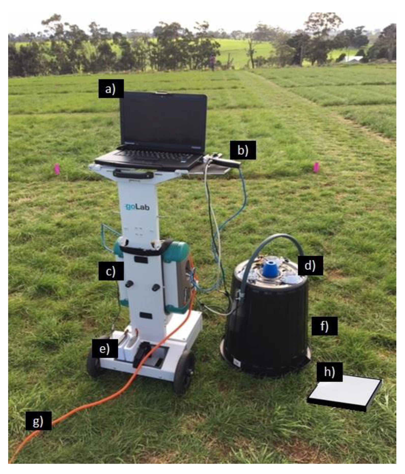
2.4. Ground-Based Spectra Collection

The spectral reflectance was sampled above each subsampling point using the ASD FieldSpec® HiRes 4 (Malvern Analytical, United Kingdom) and light-shield [12]. The FieldSpec® Hi-Res 4 provides spectral performance across the full range of the solar irradiance spectrum (350–2500 nm), and the sampling resolution of the collected spectra was 1 nm. The light-shield was made from an inverted plastic bin, painted with BLACK 2.0 (manufacturer: Culture Hustle) matte paint (Figure 2) fitted with a full spectrum of three halogen lamps [12]. The spectrometer calibration and spectra collection were controlled and saved using the ASD RS3™ software (Malvern Analytical, United Kingdom, www.malvernpanalytical.com) installed on a laptop. The reflectance value was saved into ASD file format.

2.5. Ground-Based Image Acquisition

RGB images from each sampling point were captured using a tripod-mounted digital single-lens reflex (DSLR) 12.8-megapixel camera (Model: Canon 5D, Canon Inc., Ota, Tokyo, Japan). Each RGB image was acquired 1 m above the sampling point at the nadir view before and after mechanical clipping (Figure 3). A quadrat (50 cm × 50 cm) was placed at each sampling point prior to image acquisition to maintain the same field of view in all the RGB images. The image acquisition was carried out under partially cloudy conditions to avoid shadows in the RGB images, and the tripod was maintained at the same level during image acquisition using the inbuilt levelling tool. The RGB images were saved in the jpeg file format to use in the data extraction pipeline.

Airborne Multispectral Image Acquisition

Ground Control Points (GCPs) were located within the experimental area to obtain the georectification of airborne images within 2 cm in image pre-processing steps. Multispectral images were taken before and after destructive harvesting using a RedEdge-M multispectral camera (MicaSence, Inc., Washington, United States), that was deployed using a 3DR Solo quadcopter (3D Robotics, Berkeley, CA, USA). The camera was equipped with a GNSS receiver and image location data stored in the EXIF format for each image collected. The maximum ground sampling distance of a RedEdge-M sensor is 8 cm per pixel (per band) at a 120 m height. The RedEdge-M has five narrow bands (Band 1: Blue—475 nm wavelength, 20 nm bandwidth; Band 2: Green—560 wavelength, 20 nm bandwidth; Band 3: Red—668 nm wavelength, 10 nm bandwidth; Band 4: Near Infrared—840 nm wavelength, 40 nm bandwidth; Band 5: Red Edge—717 wavelength, 10 nm bandwidth). The 3DR solo quadcopter is capable of autonomous flight and powered by 5200 mAh Li-Po Solo battery (3D Robotics, Berkeley, CA, USA), which give a flight time about 10–20 min.
The Tower 4.0.1 Beta (Aero Hawk Technologies, USA; https://aero-hawk.com/) android application was used for designing, saving, and loading the pre-designed flight path into the quadcopter and used to automate the flight during data acquisition. The turning points of the flight path were defined outside the area of interest to ensure that the whole experimental site was measured. The image overlap of the flight mission was set to 80% forward and 75% sideways, as recommended for the RedEdge-M sensor. The quadcopter was flown at an altitude of 30 m above ground level, with the ground speed of the quadcopter set to 6 ms−1 (21.6 km/h) to enable the capture of stable images. Calibration targets with known reflectance values (3%, 6%, 11%, 22%, and 33%) were kept on the ground within the field of view of the sensor during image acquisition. The reflectance value of each target was used in the data extraction workflow to convert the collected digital number values to reflectance values.

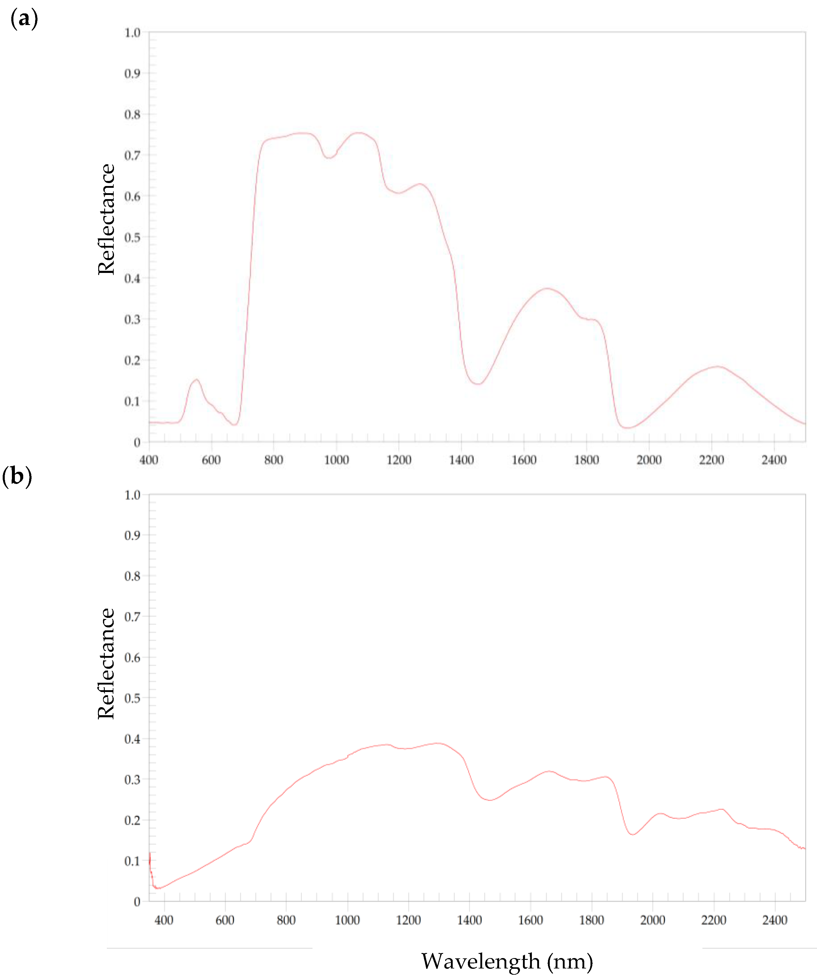
2.6. Hyperspectral Data Extraction

The spectra (ADS files) from the ASD FieldSpec® HiRes 4 were opened in the ViewSpec Pro™ software (Malvern Analytical, United Kingdom, www.malvernpanalytical.com) (Figure 4), and converted spectral information into a txt file format. Spectral data extracted to the txt file were used to calculate the following vegetation indices.
Cellulose   Absorption   Index   ( CAI ) = 0.5   ( R 2.0 + R 2.2 ) R 2.1 Normalised   Difference   Lignin   Index   ( NDLI ) = Log ( 1 R 1.7 ) Log ( 1 R 1.6 ) Log ( 1 R 1.7 ) + Log ( 1 R 1.6 ) Plant   Senecence   Reflectance   Index   ( PSRI ) = R 680 R 500 R 750
where R2.0, R2.1, R2.2, R1.7, R1.6, R680, R500, and R750 are reflectance factors in bands at 2.00–2.05, 2.08–2.13, 2.19–2.24, 1.754, 1.680, 0.680, 0.500, and 0.750 μm, respectively [30,31].

2.7. Data Extraction from Airborne Multispectral Images

A digital terrain model (DTM) and orthomosaic image of each multispectral band (green, blue, NIR, red, and red edge) were generated using the Pix4D mapper 4.2.16 software (Pix4D SA, Switzerland; https://www.pix4d.com/). The geometric calibration was performed in the Pix4D 4.2.16 software (Pix4D SA, Switzerland; https://www.pix4d.com/) workflow using 16 ground control points (GCPs) of the experimental site. The georeferencing RMS error and GSD (ground sampling distance) of the orthomosaic images were around 2 cm (Table 1). The coordinate reference system (CRS), EPSG: 32755—WGS 84/UTM zone 55S, was used as an output coordinate system for the DTM and orthomosaic images in the Pix4D workflow. The radiometric calibration for the orthomosaic images derived from the Pix4D workflow was undertaken in QGIS 2.18.20 (QGIS Development Team, 2017, Raleigh, NC, USA; https://qgis.org/) using the Zonal statistics plugin and raster calculator. The RedEdge-M multispectral camera records the intensity of the electromagnetic radiation for each pixel as a raw digital number (DN), and the radiometric calibration process converts DNs into more meaningful units, called radiance or reflectance.
The plot overlay and subsample quadrats with the same CRS were digitized, importing the calibrated orthomosaic images and the GPS location of the subsampling points into QGIS 2.18.20 (QGIS Development Team, 2017, Raleigh, NC, USA; https://qgis.org/). The orthomosaic images (raster format) of the broadband vegetation indices, listed in Table 2, were generated under the default CRS (EPSG: 32755—WGS 84/UTM zone 55S) using the raster calculator. The reflectance values of the generated vegetation indices within the digitized subsample quadrats were extracted through the Zonal statistics plugin for use in future data analysis.

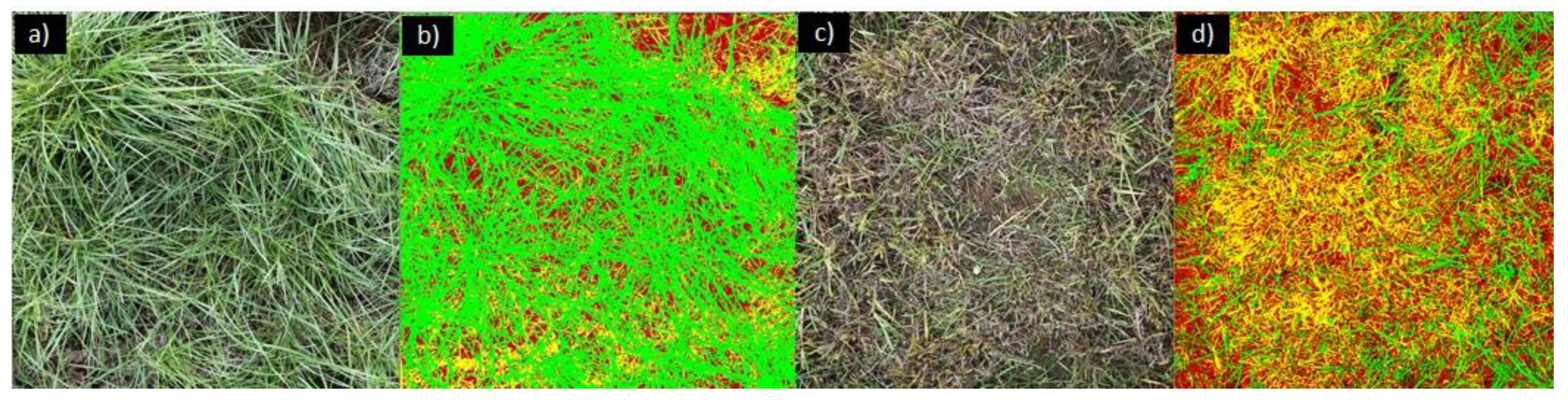
2.8. Data Extraction from Ground-Based RGB Images

Image processing was undertaken using a developed set of rules in eCognition developer 9.3.2 (Trimble Germany GmbH, Munich, Germany; http://www.ecognition.com/). The image pixels exterior to the area of interest (outside the quadrat border) of each original RGB image were removed using the ImageJ software (https://imagej.nih.gov/ij/). After image pre-processing, the raw tiff files were imported into eCognition developer 9.3.2, and an image processing algorithm, called “K-nearest neighbor” (k-NN) analysis was executed to classify the pixels into perennial ryegrass plants, soil, and senescent plant material and create a classified object layer. The accuracy of image classification was checked by analyzing the correlation coefficient of each class (living perennial ryegrass, senescent ryegrass, and soil) in the k-NN analysis workflow. The k-NN analysis is a standard machine-learning method that has been extended to large-scale data classification using a training data set. After image classification, the data was exported as a csv (comma-separated values) file using an inbuilt “export object statistics” algorithm in eCognition developer 9.3.2 (Trimble Germany GmbH, Munich, Germany; http://www.ecognition.com/).

2.9. Data Analysis

Statistical analyses were performed in Genstat 18.2.0.18409 (https://www.vsni.co.uk) and R-4.0.2 (https://cran.ms.unimelb.edu.au/). The sensor-based data were validated by performing a correlation coefficient and principal components analysis between the digital phenomics data and the manual data. The perennial ryegrass ground cover classification was predicted by fitting linear regression models between the high-throughput phenotyping data (RGB image-based ground cover classification, multispectral image-based VIs, and ground-based hyperspectral VIs) and ground truth data (manual ground cover classification and dry matter ranking data).

3. Results

3.1. Validation of K-Nearest Neighbor Analysis for Ground Cover Classification

The performance of the k-NN analysis for estimating the senescent pasture biomass is presented in Table 3. The green and senescent fractions extracted from preharvest RGB images showed a strong positive correlation with the dry matter yield of green and senescent fractions (green fraction—r = 0.665, p < 0.001; senescent fraction—r = 0.831, p < 0.001). There was a strong positive correlation between the green fraction extracted from the postharvest RGB images and the manual green fraction estimates (r = 0.774, p < 0.001). There was correlation between the perennial ryegrass senescent fraction derived from the postharvest RGB images and the manual senescent fraction estimates (r = 0.805, p < 0.001), and the postharvest RGB image-based bare ground estimates also showed a strong positive relationship with the manual bare ground estimates.

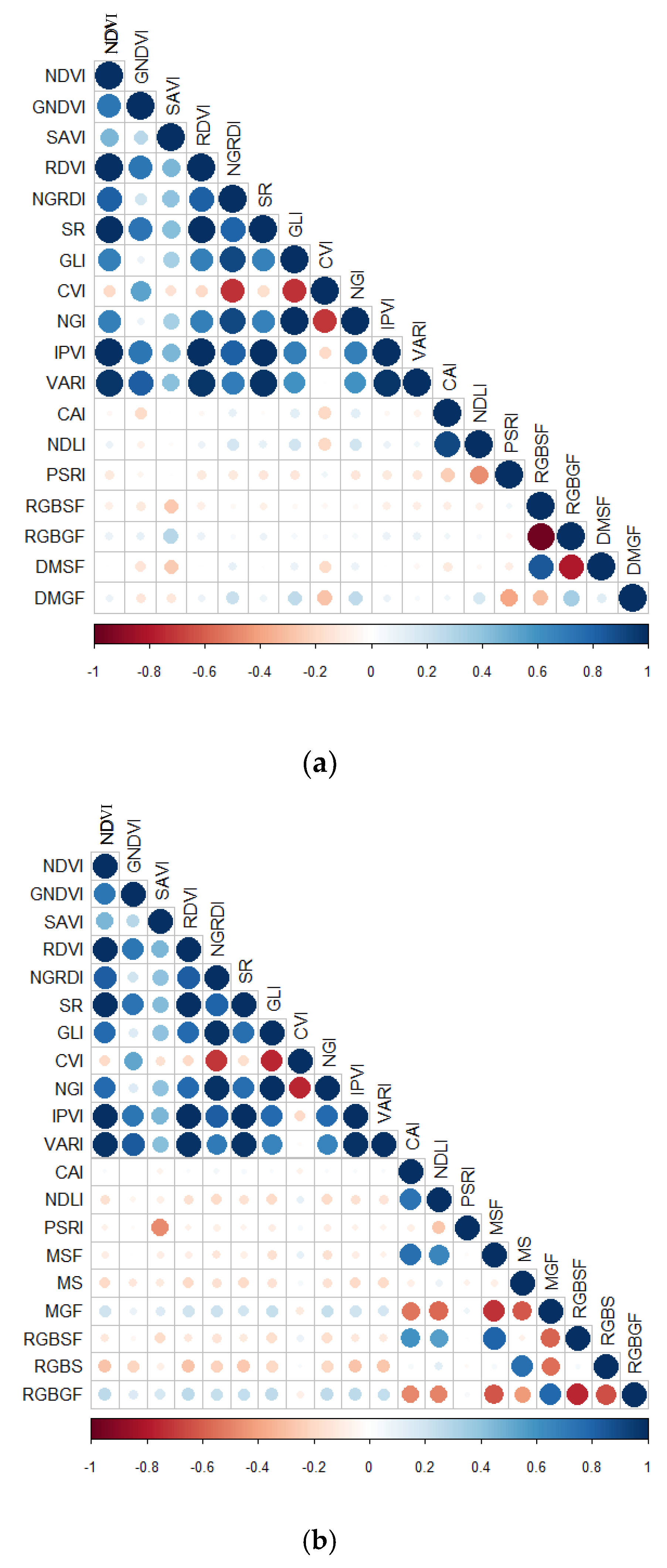
3.2. Optimum Vegetation Indices for Ground Cover Classification

As shown in Figure 5, except for the green normalized difference vegetation Index (GNDVI), green leaf index (GLI), and normalized green intensity (NGI), there was no correlation between the vegetation indices extracted from the preharvest multispectral images and the preharvest ground cover fraction of both the manual and RGB sensor-based ground fraction estimates (p > 0.05), (GNDVI vs. DMGF—r = 0.211, p > 0.01,GLI vs. DMGF—r = 0.253, p > 0.01; NGI vs. DMGF—r = 0.283, p > 0.01). Hyperspectral VI; the plant senescence reflectance index (PSRI) extracted from the preharvest field spec. data showed a negative relationship with both the RGB-sensor-based green fraction and the dry matter yield of the green fraction (PSRI vs. RGBGF—r = −0.205, p = 0.009; PSRI vs. DMGF—r = −0.395, p < 0.001). Most of the vegetation indices extracted from the postharvest multispectral images had strong positive correlations with the RGB image-derived and manually estimated green fractions (Figure 5, p < 0.05). However, there was a poor correlation between the senescent fraction (both RGB sensor-based and manual) and the pretharvest multispectral image-derived VIs (Figure 5, p < 0.05). Moreover, there was no correlation between the soil-adjusted vegetation index (SAVI) extracted from the postharvest multispectral images (Figure 5, p > 0.05). Except for the plant senescence reflectance index (PSRI), the other two tested postharvest hyperspectral VIs showed a strong positive relationship with the senescent and soil fraction estimated from the postharvest RGB images and visual estimates (Figure 5). The principal component analysis (PCA) showed a strong relationship between the VIs and ground cover classification in the post-harvest data (Figure 6).

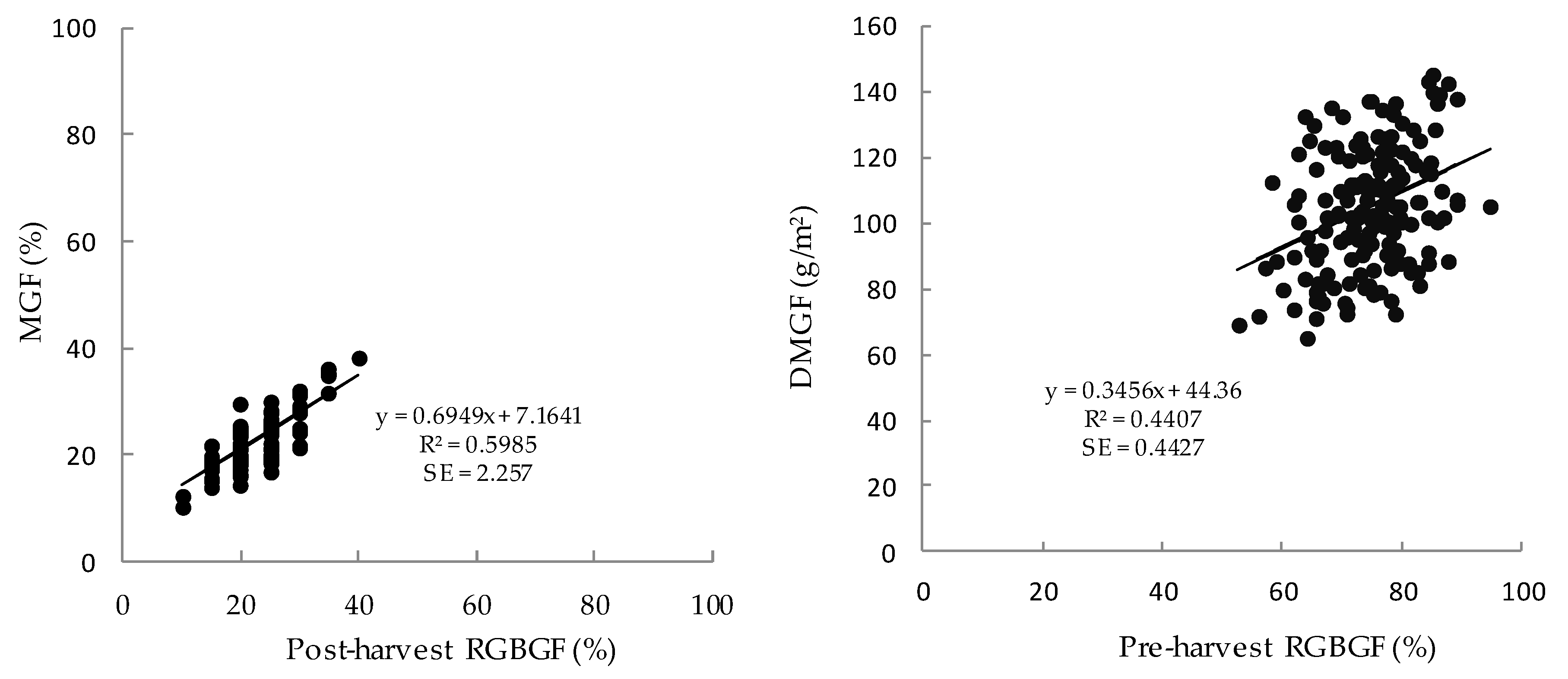
3.3. Prediction of Green Fraction (Figure 7)

3.4. Prediction of Bare Ground (Figure 8)

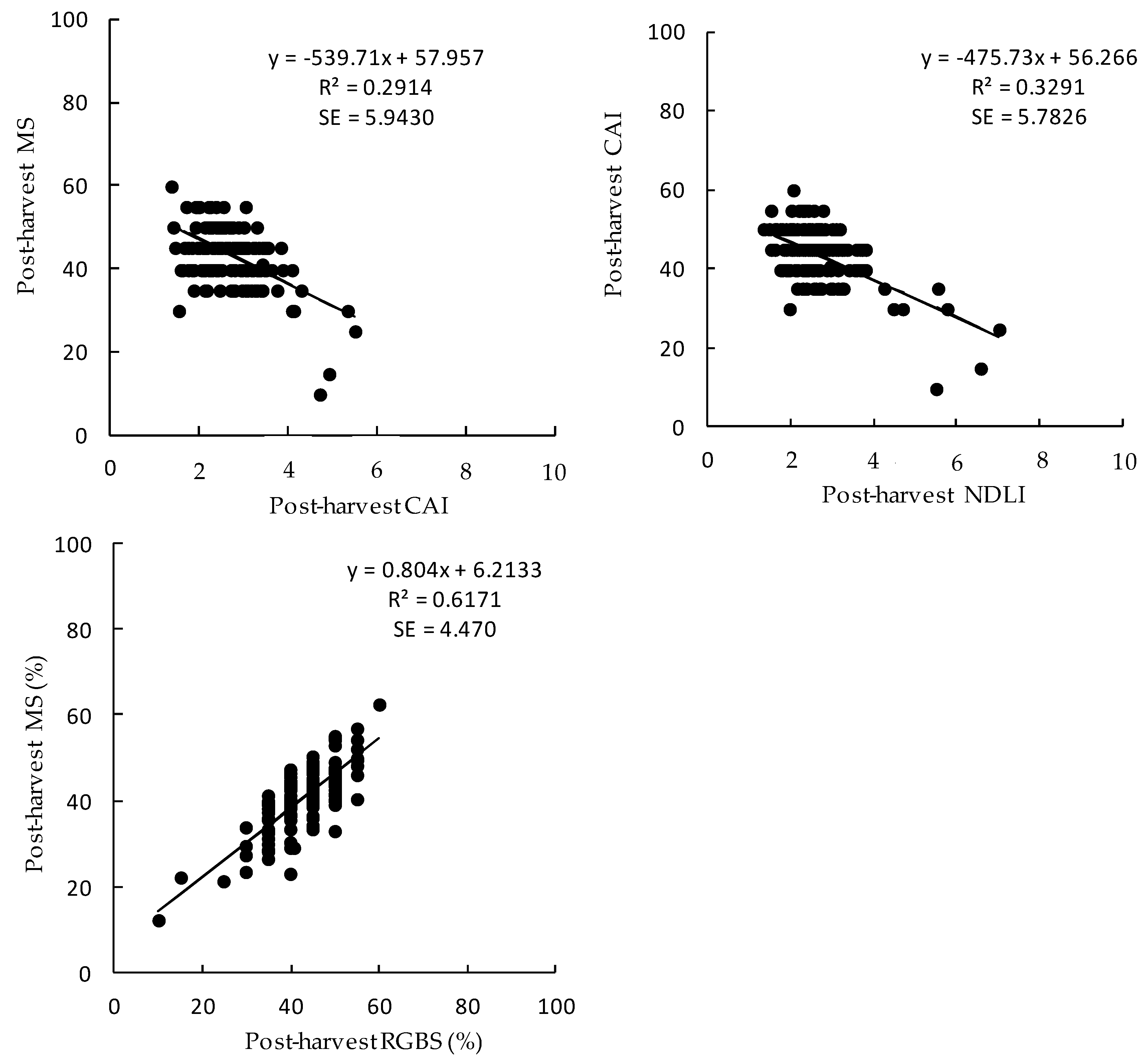
3.5. Prediction of Senescent Fraction (Figure 9)

The sensor-based phenotyping parameters showed multiple positive and negative correlations with the perennial ryegrass green and senescent fractions and bare ground estimates (Figure 5, p > 0.05), with the best combinations being for senescent, green, and bare ground predictions. As shown in Figure 7, the plot-level green fraction estimated from the postharvest RGB images showed a positive linear regression with the manual green fraction (R2 = 0.5985, p < 0.001, standard error (SE) = 2.257) estimates and the dry matter weight of green fraction (R2 = 0.4407, p < 0.001, SE = 0.4427). However, the bare ground extracted from the postharvest RGB images showed a very strong relationship with the postharvest ground cover estimates (Figure 8; R2 = 0.6176, p < 0.001, SE = 4.470). The postharvest cellulose absorption index and normalized showed a strong negative linear relationship with the postharvest manual ground cover estimation (Figure 8; MS vs. CAI—R2 = 0.2914, p < 0.001, SE = 5.9430; MS vs. NDLI—R2 = 0.3291, p < 0.001, SE = 5.7826). The best models involving senescent fraction prediction showed a strong relationship between both the pre and postharvest sensor-based and manually extracted data (Figure 9). The postharvest RGB image-based senescent fraction showed a strong linear relationship for the dry matter percentage of the senescent fraction (R2 = 0.7067, p < 0.001, SE = 4.070) and senescent fraction prediction (Figure 9; R2 = 0.6547, p < 0.001, SE = 3.083). The postharvest manual dry matter fraction and RGB image-based senescent fraction estimates were noted for the hyperspectral VIs testing for the senescent fraction prediction. The postharvest cellulose absorption index had a positive linear relation with the postharvest manual senescent fraction (R2 = 0.5707, p < 0.001, SE = 3.648) and the RGB image-based senescent fraction (R2 = 0.3685, p < 0.001, SE = 4.169), and the postharvest normalized difference lignin index also showed a positive linear regression model for senescent fraction prediction (Figure 9).

4. Discussion

This study established a sensor-based tool for ground cover classification using phenomic data acquired from both ground-based and air borne sensors. The proposed tools could overcome challenges associated with existing persistence estimation methods in large-scale pasture breeding programs, such as the discrimination of senescent pasture from bare ground. The spectral properties of bare ground and senescent pasture in the visible and near-infrared regions of EMS are similar [41]. As such, the discrimination of senescent pasture from bare ground in breeding plots is challenging using a standard image analysis process [1]. This image analysis tool could quantify the senescent pasture in the presence of living tissues and bare soil background.
Perennial ryegrass has no net growth during summer in the south-west region of Australia due to the high temperatures and water deficit. However, the opening rain and temperature decline in autumn offer perfect conditions to begin active growth in perennial ryegrass [42], which provides an ideal time to assess persistence. Therefore, data collection after autumn break is more informative for perennial ryegrass persistence estimation. Due to the active growth of perennial ryegrass after the first significant rain event in autumn, plant canopy of the breeding plots can be fully closed, and amount of the senescent plant materials under the canopy may not be visible from the top of the canopy. Therefore, manual and sensor-based phenomic data acquisition were carried out prior to and after the destructive harvest, and we have validated the pre-harvest sensor-based data using the dry weight ranking and the post-harvest sensor-based data using visual scoring [1,29]. Manual ground cover estimation can be sometimes subjective [1]. Therefore, we have increased the frequency of data points by adding three subsampling points in each plot. Moreover, the use of three independent experienced breeders for visual ground cover estimation may reduce the impact of human errors in ground truth sampling.
A study conducted on chickpeas and wheat under a controlled environment showed that quantification of plant senescence was successful using RGB-based high-throughput phenotyping [23], although the application of that pipeline may be challenging for pasture senescence estimation under field conditions. We have demonstrated a method of processing RGB images in an automated workflow that provides an accurate, rapid estimation of senescent pasture under large-scale field conditions. The positive correlation between the senescent fraction derived from RGB images and the manually estimated phenomics data such as the dry matter content of the senescent fraction and the manual senescent fraction indicated the potential of RGB images and a machine learning image analysis script for the accurate discrimination of bare ground from senescent pasture under field conditions (Figure 10). The approximately similar correlation between the preharvest RGB sensor-based ground cover and the dry matter ranking data for both senescent and green pasture may show a poor relationship between the amount of senescent and green fraction in breeding plots (Table 3). The strength of this relationship may be highly fluctuated due to the rate of senescent pasture degradation overtime. The K-nearest neighbor image analysis algorithm was used as the decision-making element to covert the RGB sensor data into a low-cost plant senescence estimating tool. The K-nearest neighbor image classification was based on thresholding the intensity level of segmented pixels using known classes (labelled manually by the user) and high-resolution images, which is essential for accurate image classification [43]. In this study, RGB images were acquired 1 m above an area of interest (nadir position) using a DSLR camera to maintain a constant pixel resolution throughout the data acquisition process. One of the disadvantages of the k-NN image classification is that it requires a high computational power to execute the script. However, this process can be sped up by reducing the training samples or increasing the image segmentation size. Proximal image acquisition from tripod mounted RGB camera would require substantial labor and time, especially in large-scale breeding programs [1]. Therefore, data acquisition needs to be modified to deploying an RGB camera on a UAV to facilitate large-scale screenings and frequent measurements from pasture breeding trials.
The incident energy absorption near 2100 nm is absent in soil reflectance spectra [16]. However, the senescent plant tissue shows absorption features around 2100, 2280, 2340, 1680, 2270, 2330 and 2380 nm due to the presence of lignin and cellulose [44] (Figure 9). The use of these absorption features may offer the possibility to discriminate senescent pasture from bare ground and living plant material. Hyperspectral VIs related to lignin and cellulose absorption features were found effective for estimation of non-photosynthetic vegetation cover in crops using satellite-based hyperspectral remote sensing [41,45]. Breeding trials of perennial ryegrass may require assessing their performance at the single plant level or row plot level for a number of years, thus the potential of satellite-based remote sensing may still be problematic due to poor spatial and temporal resolution of deployed sensors. However, this study proved that the use of a hyperspectral sensor could provide more accurate discrimination of bare ground from senescent pasture under low (~30%) vegetation cover conditions. The presence of higher amounts of green vegetation may create considerable spectral noise in the reflected spectrum due to existing cellulose, moisture and lignin of living plant material [41]. It has been shown that CAI was easily affected by green vegetation cover [45]. Preharvest green fractions of breeding plots were greater than 70%. Therefore, the preharvest hyperspectral VIs showed a poor relationship with manually estimated and RGB-based senescence fraction of pasture ground cover. However, Daughtry et al. [46] found that small fractions of green vegetation in the field of view of data acquisition have little impact on the linear relationship between CAI and the crop residue cover. The green pasture cover of sub plots was less than 30% after a destructive harvest in this study, and we have observed a strong positive relationship between the postharvest senescent fraction and the hyperspectral VIs derived from the postharvest field spec data (Figure 5). The model for bare ground prediction showed a weak negative relationship between the hyperspectral VIs and estimated soil area. Cellulose absorption features can be varied due to the soil moisture and color [41]. As such, further research is necessary to assess the performance of the hyperspectral VIs for predicting plant senescence of breeding trials under different soil and moisture conditions.
The multispectral sensor deployed on a UAV is the most common method for phenomic data acquisition in precision agriculture and offers precise phenomic data for living pasture fractional cover estimation [1]. Vegetation indices based on green fraction estimation can be limited due to the saturation of the spectral band after a certain amount of biomass density or ground cover [47]. Therefore, the preharvest broadband VIs showed a poor relationship with the preharvest ground truth data, but the broadband VIs estimated from the postharvest multispectral data indicated that spectral information acquired from broadband sensors could be used to estimate the green fraction under a low vegetation cover. Small-scale multispectral cameras such as a Micasense Red Edge sensor and a Parrot Sequoia sensor are sensitive only for a small section of EMS. These sensors acquire typically discreet broad bands like red, green, red edge, and blue, which reduces the capacity of capturing small differences in spectral properties of reflected spectra. We observed a poor correlation between broadband vegetation indices, derived from the pre and postharvest multispectral images and the manual pasture senescence estimates. This suggests that the potential of UAV-based low-cost spectral sensors is insufficient to obtain accurate estimates of canopy senescence and their dynamics. However, the relationship between broadband VIs and the senescent pasture fraction could be improved by using a high-resolution spectral camera. Broadband VIs indices like normalized difference tillage index (NDTI) and simple tillage index (STI) extracted from a satellite deployed multispectral camera were successfully used for non-photosynthetic biomass estimation in forests [48], crop fields [43] and grasslands [20]. However, the resolution of satellite VIs for estimating plant senescence at the single plant level is still challenging in precision agriculture.

5. Conclusions

Pasture senescence is an important phenotypic trait for the assessment of responses in plants to abiotic and biotic stressors. Data from ground-based and airborne sensors and image analysis software offer a platform to develop precise phenomic tools to classify perennial ryegrass ground cover for the assessment of persistence in breeding programs. This finding may support the future assessment of pasture persistence in breeding programs at a low cost from small-scale to large-scale plot trials. Visual scorings for ground cover classification could be replaced by ML-based image analysis pipeline or hyperspectral sensors without a significant loss of precision. This study showed that UAV-attached low-cost multispectral sensors may have less potential to discriminate senescent plant tissue in pasture ground cover. The findings of this study are encouraging for pasture breeders, as they imply that pasture senescence dynamics can be accurately tracked using less sophisticated and potentially cheaper spectral sensors. We conclude that the RGB-based high-throughput approach offers a fast, accurate method to assess perennial ryegrass persistence in pasture breeding programs. Improvements in spatial resolution of hyperspectral and multispectral techniques would then be used for persistence estimation in mixed swards and other monocultures.

Author Contributions

Data collection and analysis, writing—original draft preparation C.J.; review and editing, P.B., J.J., and G.S.; supervision, review, and editing, K.S.; read and approved the final manuscript, C.J., P.B., J.J., G.S., and K.S. All authors have read and agreed to the published version of the manuscript.

Funding

This research was funded by Dairy Australia, Gardiner Dairy Foundation and Agriculture Victoria Research.

Acknowledgments

We thank Elly Polonowita, Chaya Smith, Senani Karunaratne, Anna Thompson, Kelly Rentsch, Stewie Burch, and Dani Stayches for their support for data collection.

Conflicts of Interest

The authors declare no conflict of interest.

References

  1. Jayasinghe, C.; Badenhorst, P.; Wang, J.; Jacobs, J.; Spangenberg, G.; Smith, K. An Object-Based Image Analysis Approach to Assess Persistence of Perennial Ryegrass (Lolium perenne L.) in Pasture Breeding. Agronomy 2019, 9, 501. [Google Scholar] [CrossRef] [Green Version]
  2. Wilkins, P.W. Breeding perennial ryegrass for agriculture. Euphytica 1991, 52, 201–214. [Google Scholar] [CrossRef]
  3. Scott, B.; Roberts, A.; Conyers, M. Management of soil acidity in long-term pastures of south-eastern Australia: A review. Anim. Prod. Sci. 2001, 40, 1173–1198. [Google Scholar] [CrossRef]
  4. Shakhane, L.M.; Mulcahy, C.; Scott, J.M.; Hinch, G.N.; Donald, G.E.; Mackay, D.F. Pasture herbage mass, quality and growth in response to three whole-farmlet management systems. Anim. Prod. Sci. 2013, 53, 685–698. [Google Scholar] [CrossRef] [Green Version]
  5. Doyle, C.; Lazenby, A. The effect of stocking rate and fertilizer usage on income variability for dairy farms in England and Wales. Grass Forage Sci. 2006, 39, 117–127. [Google Scholar] [CrossRef]
  6. McKenzie, F.R.; Jacobs, J.L.; Kearney, G. Effects of spring grazing on dryland perennial ryegrass/white clover dairy pastures. 1. Pasture accumulation rates, dry matter consumed yield, and nutritive characteristics. Aust. J. Agric. Res. 2006, 57, 543–554. [Google Scholar] [CrossRef]
  7. Malcolm, B.; Smith, K.F.; Jacobs, J.L. Perennial pasture persistence: The economic perspective. Crop Pasture Sci. 2014, 65, 713–720. [Google Scholar] [CrossRef]
  8. Woodward, S.J.R. Quantifying different causes of leaf and tiller death in grazed perennial ryegrass swards. N. Z. J. Agric. Res. 1998, 41, 149–159. [Google Scholar] [CrossRef]
  9. Allen, V.G.; Batello, C.; Berretta, E.J.; Hodgson, J.; Kothmann, M.; Li, X.; McIvor, J.; Milne, J.; Morris, C.; Peeters, A.; et al. An international terminology for grazing lands and grazing animals. Grass Forage Sci. 2011, 66, 2–28. [Google Scholar] [CrossRef]
  10. Makanza, R.; Zaman-Allah, M.; Cairns, J.E.; Magorokosho, C.; Tarekegne, A.; Olsen, M.; Prasanna, B.M. High-Throughput Phenotyping of Canopy Cover and Senescence in Maize Field Trials Using Aerial Digital Canopy Imaging. Remote Sens. 2018, 10, 330. [Google Scholar] [CrossRef] [Green Version]
  11. Gebremedhin, A.; Badenhorst, P.E.; Wang, J.; Spangenberg, G.C.; Smith, K.F. Prospects for Measurement of Dry Matter Yield in Forage Breeding Programs Using Sensor Technologies. Agronomy 2019, 9, 65. [Google Scholar] [CrossRef] [Green Version]
  12. Smith, C.; Cogan, N.; Badenhorst, P.; Spangenberg, G.; Smith, K. Field Spectroscopy to Determine Nutritive Value Parameters of Individual Ryegrass Plants. Agronomy 2019, 9, 293. [Google Scholar] [CrossRef] [Green Version]
  13. Borra-Serrano, I.; De Swaef, T.; Aper, J.; Ghesquiere, A.; Mertens, K.; Nuyttens, D.; Saeys, W.; Somers, B.; Vangeyte, J.; Roldán-Ruiz, I.; et al. Towards an objective evaluation of persistency of Lolium perenne swards using UAV imagery. Euphytica 2018, 214, 142. [Google Scholar] [CrossRef]
  14. Aase, J.K.; Tanaka, D.L. Reflectances from Four Wheat Residue Cover Densities as Influenced by Three Soil Backgrounds. Agron. J. 1991, 83, 753–757. [Google Scholar] [CrossRef]
  15. Qi, J.; Marsett, R.; Heilman, P.; Bieden-bender, S.; Moran, S.; Goodrich, D.; Weltz, M. RANGES improves satellite-based information and land cover assessments in southwest United States. Eos Trans. Am. Geophys. Union 2002, 83, 601–606. [Google Scholar] [CrossRef]
  16. Daughtry, C. Discriminating Crop Residues from Soil by Shortwave Infrared Reflectance. Agron. J. 2001, 93, 125–131. [Google Scholar] [CrossRef]
  17. Ren, H.; Zhou, G.; Zhang, F.; Zhang, X. Evaluating cellulose absorption index (CAI) for non-photosynthetic biomass estimation in the desert steppe of Inner Mongolia. Chin. Sci. Bull. 2012, 57, 1716–1722. [Google Scholar] [CrossRef] [Green Version]
  18. Roberts, D.A.; Smith, M.O.; Adams, J.B. Green vegetation, nonphotosynthetic vegetation, and soils in AVIRIS data. Remote Sens. Environ. 1993, 44, 255–269. [Google Scholar] [CrossRef]
  19. Daughtry, C.S.T.; McMurtrey, J.E.; Chappelle, E.W.; Hunter, W.J.; Steiner, J.L. Measuring crop residue cover using remote sensing techniques. Theor. Appl. Climatol. 1996, 54, 17–26. [Google Scholar] [CrossRef]
  20. Ren, S.; Chen, X.; An, S. Assessing plant senescence reflectance index-retrieved vegetation phenology and its spatiotemporal response to climate change in the Inner Mongolian Grassland. Int. J. Biometeorol. 2017, 61, 601–612. [Google Scholar] [CrossRef]
  21. Kim, J.Y. Roadmap to High Throughput Phenotyping for Plant Breeding. J. Biosyst. Eng. 2020, 45, 43–55. [Google Scholar] [CrossRef]
  22. Daughtry, C.S.T.; McMurtrey, J.E.; Kim, M.S.; Chappelle, E.W. Estimating crop residue cover by blue fluorescence imaging. Remote Sens. Environ. 1997, 60, 14–21. [Google Scholar] [CrossRef]
  23. Cai, J.; Okamoto, M.; Atieno, J.; Sutton, T.; Li, Y.; Miklavcic, S.J. Quantifying the Onset and Progression of Plant Senescence by Color Image Analysis for High Throughput Applications. PLoS ONE 2016, 11, e0157102. [Google Scholar] [CrossRef] [PubMed] [Green Version]
  24. Beggan, C.; Hamilton, C. New image processing software for analyzing object size-frequency distributions, geometry, orientation, and spatial distribution. Comput. Geosci. 2009, 36, 539–549. [Google Scholar] [CrossRef]
  25. Bieniecki, W.; Grabowski, S. Nearest neighbor classifiers for color image segmentation. In Proceedings of the International Conference Modern Problems of Radio Engineering, Telecommunications and Computer Science, Lviv-Slavsko, Ukraine, 28 February 2004. [Google Scholar] [CrossRef]
  26. Dingle Robertson, L.; King, D.J. Comparison of pixel- and object-based classification in land cover change mapping. Int. J. Remote Sens. 2011, 32, 1505–1529. [Google Scholar] [CrossRef]
  27. Rehman, T.; Mahmud, M.; Chang, Y.; Jin, J.; Shin, J. Current and future applications of statistical machine learning algorithms for agricultural machine vision systems. Comput. Electron. Agric. 2018, 156, 585–605. [Google Scholar] [CrossRef]
  28. McCormick, L.H.; Lodge, G.M. A field kit for producers to assess pasture health in the paddock. In Proceedings of the 10th Australian Agronomy Conference, Hobart, Tasmania, 28 January–1 February 2001. [Google Scholar]
  29. Mannetje, L.; Haydock, K.P. The dry-weight-rank method for the botanical analysis of pasture. Grass Forage Sci. 1963, 18, 268–275. [Google Scholar] [CrossRef]
  30. Erdle, K.; Mistele, B.; Schmidhalter, U. Comparison of active and passive spectral sensors in discriminating biomass parameters and nitrogen status in wheat cultivars. Field Crops Res. 2011, 124, 74–84. [Google Scholar] [CrossRef]
  31. Hunt, R.; Hively, W.; McCarty, G.; Daughtry, C.; Forrestal, P.; Kratochvil, R.; Carr, J.; Allen, N.; Fox-Rabinovitz, J.; Miller, C. NIR-Green-Blue High-Resolution Digital Images for Assessment of Winter Cover Crop Biomass. GISci. Remote Sens. 2011, 48, 86–98. [Google Scholar] [CrossRef]
  32. Haboudane, D.; Miller, J.R.; Tremblay, N.; Zarco-Tejada, P.J.; Dextraze, L. Integrated narrow-band vegetation indices for prediction of crop chlorophyll content for application to precision agriculture. Remote Sens. Environ. 2002, 81, 416–426. [Google Scholar] [CrossRef]
  33. Fu, Y.; Yang, G.; Wang, J.; Feng, H. A comparative analysis of spectral vegetation indices to estimate crop leaf area index. Intell. Autom. Soft Comput. 2013, 19, 315–326. [Google Scholar] [CrossRef]
  34. Prabhakara, K.; Hively, W.D.; McCarty, G.W. Evaluating the relationship between biomass, percent groundcover and remote sensing indices across six winter cover crop fields in Maryland, United States. Int. J. Appl. Earth Obs. Geoinf. 2015, 39, 88–102. [Google Scholar] [CrossRef] [Green Version]
  35. Jordan, C.F. Derivation of Leaf-Area Index from Quality of Light on the Forest Floor. Ecology 1969, 50, 663–666. [Google Scholar] [CrossRef]
  36. Louhaichi, M.; Borman, M.M.; Johnson, D.E. Spatially Located Platform and Aerial Photography for Documentation of Grazing Impacts on Wheat. Geocarto Int. 2001, 16, 65–70. [Google Scholar] [CrossRef]
  37. Vincini, M.; Frazzi, E. Comparing narrow and broad-band vegetation indices to estimate leaf chlorophyll content in planophile crop canopies. Precis. Agric. 2011, 12, 334–344. [Google Scholar] [CrossRef]
  38. Woebbecke, D.M.; Meyer, G.E.; Von Bargen, K.; Mortensen, D.A. Color Indices for Weed Identification Under Various Soil, Residue, and Lighting Conditions. Trans. ASAE 1995, 38, 259–269. [Google Scholar] [CrossRef]
  39. Payero, J.O.; Christopher, N.; Wright, J.L. Comparison of eleven vegetation indices for estimating plant height of alfalfa and grass. Appl. Eng. Agric. 2004, 20, 385–393. [Google Scholar] [CrossRef] [Green Version]
  40. Gitelson, A.A.; Kaufman, Y.J.; Stark, R.; Rundquist, D. Novel algorithms for remote estimation of vegetation fraction. Remote Sens. Environ. 2002, 80, 76–87. [Google Scholar] [CrossRef] [Green Version]
  41. Nagler, P.; Inoue, Y.; Glenn, E.; Russ, A.; Daughtry, C. Cellulose absorption index (CAI) to quantify mixed soil–plant litter scenes. Remote Sens. Environ. 2003, 87, 310–325. [Google Scholar] [CrossRef]
  42. Waller, R.A.; Sale, P.W.G. Persistence and productivity of perennial ryegrass in sheep pastures in south-western Victoria: A review. Aust. J. Exp. Agric. 2001, 41, 117–144. [Google Scholar] [CrossRef]
  43. Najafi, P.; Navid, H.; Feizizadeh, B.; Eskandari, I. Remote sensing for crop residue cover recognition: A review. Agric. Eng. Int. CIGR E-J. 2018, 20, 63–69. [Google Scholar]
  44. Bannari, A.; Staenz, K.; Khurshid, K.S. Remote sensing of crop residue using Hyperion (EO-1) data. In Proceedings of the IEEE International Geoscience & Remote Sensing Symposium, Barcelona, Spain, 23–28 July 2007; pp. 2795–2799. [Google Scholar]
  45. Daughtry, C.; Hunt, E.R.; Doraiswamy, P.C.; McMurtrey, J.E. Remote Sensing the Spatial Distribution of Crop Residues. Agron. J. 2005, 97, 864–871. [Google Scholar] [CrossRef]
  46. Daughtry, C.S.T.; Hunt, E.R.; McMurtrey, J.E. Assessing crop residue cover using shortwave infrared reflectance. Remote Sens. Environ. 2004, 90, 126–134. [Google Scholar] [CrossRef]
  47. Zhao, F.; Xu, B.; Yang, X.; Jin, Y.; Li, J.; Xia, L.; Chen, S.; Ma, H. Remote Sensing Estimates of Grassland Aboveground Biomass Based on MODIS Net Primary Productivity (NPP): A Case Study in the Xilingol Grassland of Northern China. Remote Sens. 2014, 6, 5368–5386. [Google Scholar] [CrossRef] [Green Version]
  48. Higgins, M.A.; Asner, G.P.; Perez, E.; Elespuru, N.; Alonso, A. Variation in photosynthetic and nonphotosynthetic vegetation along edaphic and compositional gradients in northwestern Amazonia. Biogeosciences 2014, 11, 3505–3513. [Google Scholar] [CrossRef] [Green Version]
Figure 1. (a) Preharvest composite RGB orthomosaic of experimental site; (b) the expanded area of the study site (red transparent area of image (a)), where black color polygons represent the boundaries of the experimental plot and red color polygons represent the subsampling locations in each plot.
Agronomy 10 01206 g001
Figure 2. The ASD FieldSpec® HiRes 4 spectroradiometer setup for spectra collection in field conditions. (a) Field laptop; (b) 10° lens, scrambler, and pistol-grip; (c) the FieldSpec® Hi-Res 4; (d) halogen lights; (e) energy supply for the spectroradiometer; (f) light-shield; (g) power supply to the light-shield; and (h) Spectralon® reference panel.
Agronomy 10 01206 g002
Figure 3. (a) Camera arrangement for RGB image acquisition at a sampling point, (b) preharvest RGB image of a sampling point (c) postharvest RGB image of the same sampling point.
Agronomy 10 01206 g003
Figure 4. The spectral reflectance of a perennial ryegrass breeding plot, (a) before and (b) after the destructive harvest, where the spectra were generated using the ASD FieldSpec® HiRes 4 hyperspectral data with no derivatives.
Agronomy 10 01206 g004
Figure 5. The correlogram for ground cover fractions and vegetation indices; plot (a) shows the preharvest data and plot (b) represents the postharvest data. Positive correlations are displayed in blue and negative correlations in red color. Color intensity and the size of the circle are proportional to the correlation coefficients. MSF is manual senescent fraction, MGF is manual green fraction, MS is manual soil cover, RGBSF is RGB sensor-based senescent fraction, RGBGF is RGB sensor-based green fraction, and RGBS is RGB sensor-based soil cover. DMSF is the dry matter percentage of the senescent fraction, and DMGF is the dry matter percentage of the green fraction.
Agronomy 10 01206 g005
Figure 6. The principal component analysis. The loading plots of the components 1 and 2 obtained from the ground cover fractions and vegetation indices; plot (a) shows the preharvest data and plot (b) represents the postharvest data. MSF is manual senescent fraction, MGF is manual green fraction, MS is manual soil cover, RGBSF is RGB sensor-based senescent fraction, RGBGF is RGB sensor-based green fraction, and RGBS is RGB sensor-based soil cover. DMSF is the dry matter percentage of the senescent fraction, and DMGF is the dry matter percentage of the green fraction.
Agronomy 10 01206 g006
Figure 7. Linear regression models for green fraction prediction, n = 162, where RGBGF is RGB image-based green fraction, MGF is manual green fraction, and DMGF is the dry matter of the green fraction.
Agronomy 10 01206 g007
Figure 8. Linear regression for bare ground prediction, n = 162, where MS is manual soil area, RGBSF is RGB image-based soil area, CAI is cellulose absorption index, and NDLI is normalized difference lignin index.
Agronomy 10 01206 g008
Figure 9. Linear regression for the plot-level perennial ryegrass dead fraction prediction, n = 162, where MSF is the manual senescent fraction, DMSF is the dry matter of the senescent fraction, RGBSF is the RGB image-based senescent fraction, CAI is the cellulose absorption index, and NDLI is the normalized difference lignin index.
Agronomy 10 01206 g009
Figure 10. K-nearest neighbor image classification of preharvest (a) and postharvest (c) images of the same plot (plot no 8); (b,d) are classified images of original images, where green color represents living pasture, yellow color represents senescent pasture, and brown color area is bare ground.
Agronomy 10 01206 g010
Table 1. Details of UAV image acquisition and orthomosaic quality summary.
FlightImage Overlap
Forward/Side
Flight Speed
(m/s)
Flight Height
(m)
Georeferencing Mean RMS Error (m)GSD
(cm/pixels)
Pre-harvest80%/75%6300.0192.26
Post-harvest80%/75%6300.0102.16
Table 2. List of the broadband vegetation indices used in this study.
Vegetation IndexAbbreviationEquation
Normalised Difference Vegetation IndexNDVI(Rn − Rr)/(Rn + Rr) [11,30]
Green Normalised Difference Vegetation IndexGNDVI(Rn − Rg)/(Rn + Rg) [31]
Soil Adjusted Vegetation IndexSAVI(Rn − Rr)/(Rn + Rr + 0.5) × (1 + 0.5) [32]
Renormalised Difference Vegetation IndexRDVI(Rn − Rr)/(Rn + Rr)1/2 [33]
Normalised green-Red difference indexNGRDI(Rg − Rr)/(Rg + Rr)1/2 [34]
Simple Ratio IndexSRIRn/Rr [35]
Green Leaf indexGLI(2 × Rg − Rr − Rb)/(2 × Rg + Rr + Rb) [36]
Chlorophyll Vegetation IndexCVIRn × Rr/Rg2 [37]
Normalised Green IntensityNGIRg/(Rr + Rg + Rb) [38]
Infrared Percentage Vegetation IndexIPVIRn/(Rn + Rr) [39]
Visible Atmospherically Resistant IndexVARI(Rn − Rr)/(Rr + Rg + Rb) [40]
Rn is the near infrared band reflectance, Rr is the red band reflectance, Rg is the green band reflectance, and Rb is the blue band reflectance.
Table 3. The comparison of the manual and RGB sensor-based ground cover classification.
ParameterSpearman’s Correlationp-Value
RGBSF vs DMSF (Preharvest)0.831<0.001
RGBGF vs. DMGF (Preharvest)0.665<0.001
RGBSF vs MSF (Postharvest)0.805<0.001
RGBGF vs. MGF (Postharvest)0.774<0.001
RGBS vs. MS (Postharvest)0.782<0.001
DMSF is the dry matter percentage of senescent fraction, DMGF is the dry matter percentage of green fraction, RGBDF is the RGB sensor-based senescent fraction, RGBGF is the RGB sensor-based green fraction, RGBS is the RGB sensor-based soil cover, MSF is the manual senescent fraction, MGF is the manual green fraction, and MS is the manual soil cover.

