Distributed Passive Actuation Schemes for Seismic Protection of Multibuilding Systems

Abstract

In this paper, we investigate the design of distributed damping systems (DDSs) for the overall seismic protection of multiple adjacent buildings. The considered DDSs contain interstory dampers implemented inside the buildings and also interbuilding damping links. The design objectives include mitigating the buildings seismic response by reducing the interstory-drift and story-acceleration peak-values and producing small interbuilding approachings to decrease the risk of interbuilding collisions. Designing high-performance DDS configurations requires determining convenient damper positions and computing proper values for the damper parameters. That allocation-tuning optimization problem can pose serious computational difficulties for large-scale multibuilding systems. The design methodology proposed in this work—(i) is based on an effective matrix formulation of the damped multibuilding system; (ii) follows an $H_{\infty }$ approach to define an objective function with fast-evaluation characteristics; (iii) exploits the computational advantages of the current state-of-the-art genetic algorithm solvers, including the usage of hybrid discrete-continuous optimization and parallel computing; and (iv) allows setting actuation schemes of particular interest such as full-linked configurations or nonactuated buildings. To illustrate the main features of the presented methodology, we consider a system of five adjacent multistory buildings and design three full-linked DDS configurations with a different number of actuated buildings. The obtained results confirm the flexibility and effectiveness of the proposed design approach and demonstrate the high-performance characteristics of the devised DDS configurations.

1. Introduction

Over the last few years, an increasing research effort has been invested in the analysis, design and implementation of distributed damping systems (DDSs) for seismic protection of buildings and civil structures [1,2]. That kind of passive energy-dissipation systems is formed by a set of damping elements installed at suitable locations of the structure. DDSs are simple, reliable and robust and, when properly designed, are able to produce a remarkable reduction of the overall seismic vibrational response [3,4,5]. Broadly speaking, three main issues related to the damping elements have to be addressed in DDS design—(i) technical setup determination, (ii) allocation and (iii) tuning. Determination of the technical setup is a preliminary step, which is strongly conditioned by the particular problem under consideration and involves selecting a particular kind of damping devices and, possibly, setting other technical characteristics such as the type of damper mounting, maximum damping capacity or maximum stroke [6,7]. It can also include some overall characteristics as the total number of allowed dampers or the overall damping capacity. The allocation problem requires determining a suitable set of structural positions to implement the dampers, and the tuning problem consists in computing adequate values for the damper parameters. For a given technical setup, the allocation and tuning issues are clearly interlinked and both must be simultaneously solved in order to obtain a DDS design with high-performance characteristics. The combined allocation-tuning problem can be formulated as a constrained optimization problem, with a set of decision variables that describes the different allocation schemes and parameter values of the damping devices, an objective function that allows evaluating the suitability of the corresponding DDSs, and a system of constraints that incorporate relevant features of the considered technical setup. To solve allocation-tuning optimization problems (ATOPs), a wide variety of computational strategies have been proposed, which include specialized optimization methods [8,9,10,11,12] and adaptations of general-purpose optimization algorithms [13,14,15]. Specialized optimization methods are specifically designed for particular kinds of ATOPs and, sometimes, can produce remarkably effective results for the considered problem. However, it should be highlighted that solving ATOPs for large structural systems can be a hard computational task, due to a number of factors such as high dimensionality, the combination of discrete and continuous decision variables, the presence of complex structural constraints, and the computational cost associated to the evaluation of the objective function. In this context, taking advantage of state-of-the-art general-purpose optimization solvers can be an element of critical relevance.

The general goal of the paper is to design high-performance DDSs for seismic protection of multibuilding systems (MBSs) formed by a row of m adjacent buildings as the one schematically displayed in Figure 1. There certainly exists a large number of works on DDS design for single buildings in the literature; some recent discussions on the topic can be found in References [5,6,7,15,16]. For the particular case of $m=2$ adjacent buildings, the number of references is remarkably smaller but yet significant. Works in this line include different kinds of interbuilding damping devices [17,18,19] and actuation schemes [20,21,22]. In contrast, to our best knowledge, the more general case of DDS design for MBSs with $m\ge 3$ adjacent buildings remains practically unexplored.

To keep the complexity of the considered problem within a reasonable level, in this work we assume that all the buildings have identical dynamic characteristics [20,21]. That choice allows simplifying the notations in the overall mathematical model and can help to clarify the effects produced by the DDS, which otherwise could be confounded by the action of the distinct building responses. Moreover, as rows of adjacent identical buildings is a quite common arrangement in residential areas, the selected MBS configuration can be considered as a case of potential practical interest [23]. Also for simplicity, the buildings are modeled as linear planar frames and the damping devices are assumed to be fluid viscous dampers (FVDs), which have proved to be effective energy-dissipation elements in structural vibration control and bring the modeling advantage of admitting a reasonably linear representation [7]. Attending to the structural placement, the DDS can contain two different kinds of dampers—(i) interstory dampers, which are implemented between consecutive stories of the same building and produce a resistant force proportional to the corresponding interstory velocity and (ii) interbuilding dampers, which are implemented as linking elements between stories located at the same level in adjacent buildings and produce a resistant force proportional to the relative velocity of the linked stories. The DDS can also include two types of building damping configurations of particular interest—(i) nonactuated buildings, which do not contain any interstory damper and (ii) linked buildings, which are linked to all their adjacent buildings by means of interbuilding dampers. For instance, in the MBS presented in Figure 1, buildings ${\mathcal{B}}^{\left(2\right)}$ and ${\mathcal{B}}^{\left(3\right)}$ are nonactuated; buildings ${\mathcal{B}}^{\left(1\right)}$, ${\mathcal{B}}^{\left(2\right)}$ and ${\mathcal{B}}^{\left(3\right)}$ are linked; ${\mathcal{B}}^{\left(4\right)}$ is only partially linked and ${\mathcal{B}}^{\left(5\right)}$ is unlinked. It should be observed that the DDS implementation can be carried out without internal modifications of nonactuated buildings, which can be an important factor in retrofitting. The relevance of linked configurations lies in the fact that they can help to mitigate the vibrational response of nonactuated buildings and can also provide an effective protection against interbuilding impacts (pounding) [22,23]. To incorporate those aspects in the DDS design and reducing the number of optimization variables, we introduce the schemes of allowed damper positions, which specify the interstory and interbuilding locations where the dampers can be implemented. Finally, we complete the technical setup determination by setting the maximum damping capacity of the dampers, the overall maximum damping capacity of the DDS and the total number of allowed damping elements.

In order to define the ATOP, the generic goal of improving the overall seismic response of the MBS is formulated as a triplet of particular design objectives: (i) reducing the magnitude of the buildings interstory drifts, (ii) reducing the magnitude of the buildings floor accelerations and (iii) reducing the interbuilding approachings. Objectives (i) and (ii) are applicable to single-building designs, and are respectively associated to the protection of the buildings structural and nonstructural elements [16,24]. Objective (iii) is specific to MBS designs and is associated to avoiding interbuilding impacts, which can produce severe damage to both structural and nonstructural elements. In order to obtain a computationally effective procedure, we select the overall vector of interstory drifts as controlled output and follow a single-objective $H_{\infty }$ approach [25,26]. That choice sets the reduction of interstory drifts as the primary objective and, at the same time, is able to produce positive results in mitigating the story accelerations [22]. As for design objective (iii), reduction of interbuilding approachings can be attained by enforcing a full-linked configuration in the optimization constraints [27,28]. Computationally, the selected $H_{\infty }$ objective-function avoids conducting numerical simulations of seismic time-responses and admits a fast evaluation using the hinfnorm function of the Matlab Robust Control Toolbox [29,30]. The ATOP solutions are obtained with the genetic algorithm (GA) solver provided by the Matlab Global Optimization Toolbox, which allows using hybrid sets of discrete and continuous optimization variables, permits defining a sufficiently wide variety of optimization constraints and facilitates an easy implementation of parallel computing [31]. To demonstrate the flexibility of the proposed methodology, three different DDSs are designed for the seismic protection of a MBS formed by $m=5$ adjacent five-story buildings. After that, a proper set of numerical simulations are conducted using the full-scale 180-component of the El Centro 1940 seismic record as ground acceleration disturbance. The obtained results corroborate the effectiveness of the proposed design procedure and confirm its computational efficiency for large-scale problems.

The content of the rest of the paper is as follows—in Section 2, a general mathematical model for plain and damped MBSs is presented. The main elements of the optimization procedure are discussed in Section 3. In Section 4, three different DDSs for a five-building system are designed. In Section 5, the corresponding seismic time-responses are computed and compared. Finally, in Section 6, some brief conclusions and future research lines are provided.

Remark 1.

To reduce the problem complexity and facilitate an effective computational solution, a number of model simplifications have been introduced in the paper, which should be carefully considered for a proper understanding of the scope and applicability of the proposed design methodology. Specifically, buildings are considered as linear multistory planar frames with stories of the same height. In the multibuilding systems, all the buildings are identical, with the same mass, stiffness and damping matrices, and there are no vertical differences between stories placed at the same level in different buildings. The damping elements are ideal linear dampers and the damping constants can take any real value in a prescribed interval. The interbuilding separations are assumed to be large enough to avoid interbuilding impacts. Additionally, the effect of some relevant elements such as the soil-structure interaction and the seismic wave propagation have been neglected.

Remark 2.

The considered problem requires a complex system of notations. To obtain a more organized and clear presentation, throughout this paper symbols related to interstory elements will be usually marked with hats and those corresponding to interbuilding elements will be signaled with tildes. When convenient, overlines will be used to distinguish some elements related to the overall MBS. Thus, for example, ${\widehat{n}}_j$ will denote the number of interstory dampers in building ${\mathcal{B}}^{\left(j\right)}$, the number of interbuilding dampers between buildings ${\mathcal{B}}^{\left(j\right)}$ and ${\mathcal{B}}^{(j+1)}$ will be indicated by ${\tilde{n}}_j$, and the overall number of degrees of freedom in the MBS will be represented by $\overline{n}$.

2. Mathematical Model

In this section we present mathematical models for the dynamical response of MBSs equipped with a distributed set of interstory and interbuilding FVDs. The proposed models are fully formulated in matrix form and include state-space representations to facilitate an efficient computational implementation, which is a factor of critical relevance in the practical application of the design procedure.

2.1. Plain Building Model

Let us consider a MBS system formed by a row of m adjacent n-story buildings with identical dynamic characteristics. In the plain configuration, we assume that the buildings damping is only due to the effect of the structural damping, and the dynamical response of building ${\mathcal{B}}^{\left(j\right)}$ can be modeled in the following form:

$${\mathbf{M}}_b{\ddot{\mathbf{q}}}^{\left(j\right)}\left(t\right)+{\mathbf{C}}_b{\dot{\mathbf{q}}}^{\left(j\right)}\left(t\right)+{\mathbf{K}}_b{\mathbf{q}}^{\left(j\right)}\left(t\right)=-{\mathbf{M}}_b{\left[\mathbf{1}\right]}_{n\times 1}\ddot{w}\left(t\right),$$

(1)

where ${\mathbf{q}}^{\left(j\right)}\left(t\right)={[q_1^j\left(t\right),\dots ,q_n^j\left(t\right)]}^T$ is the vector of story displacements with respect to the ground (see Figure 2); ${\mathbf{M}}_b$, ${\mathbf{C}}_b$ and ${\mathbf{K}}_b$ are the building mass, damping and stiffness matrices, respectively, which are common to all the buildings; ${\left[\mathbf{1}\right]}_{n\times 1}$ is a column vector of size n with all its entries equal to one; and $\ddot{w}\left(t\right)$ is the acceleration of the seismic ground disturbance. The building mass matrix has the diagonal form

$${\mathbf{M}}_b=\mathrm{diag}[m_1,\dots ,m_n]=\left[\begin{array}{cc}{m}_1& \\ & \ddots \\ & & m_n\end{array}\right],$$

(2)

where $m_i$ is the mass of the ith story. The stiffness matrix has the following tridiagonal structure:

$${\mathbf{K}}_b=\left[\begin{array}{ccccc}{k}_1+k_2& -k_2& & & \\ -k_2& k_2+k_3& -k_3& & \\ & \dots & \dots & \dots & \\ & & -k_{n-1}& k_{n-1}+k_n& -k_n\\ & & & -k_n& \phantom{-}{k}_n\end{array}\right],$$

(3)

where $k_i$ is the stiffness coefficient of the ith story. The stiffness matrix can be computed in the form

$${\mathbf{K}}_b=\mathbf{P}\mathrm{diag}[k_1,\dots ,k_n]{\mathbf{P}}^T,$$

(4)

where $\mathrm{diag}[k_1,\dots ,k_n]$ is the diagonal matrix defined by the story stiffness coefficients and $\mathbf{P}\in {\mathbb{R}}^{n\times n}$ is the upper band-diagonal matrix

$$\mathbf{P}=\left[\begin{array}{ccccc}1& -1& & & \\ & \phantom{-}1& -1& & \\ & & \dots & \dots & \\ & & & 1& -1\\ & & & & \phantom{-}1\end{array}\right],$$

(5)

with the following elements:

$$\left\{\begin{array}{cc}{\left[P\right]}_{i,i}=1,\hfill & i=1,\dots ,n,\hfill \\ {\left[P\right]}_{i,i+1}=-1,\hfill & i=1,\dots ,n-1,\hfill \\ {\left[P\right]}_{i,j}=0,\hfill & \mathrm{otherwise}.\hfill \end{array}\right.$$

(6)

When the story damping coefficients $c_i,i=1,\dots ,n$ are known, the structure of the building damping matrix ${\mathbf{C}}_b$ is similar to the structure of the stiffness matrix in Equation (3) and can be computed in the following form:

$${\mathbf{C}}_b=\mathbf{P}\mathrm{diag}[c_1,\dots ,c_n]{\mathbf{P}}^T.$$

(7)

Frequently, however, the damping coefficients $c_i$ cannot be properly determined and an approximate damping matrix ${\mathbf{C}}_b$ is computed by setting a suitable damping ratio on some of the building vibration modes [32]. Specifically, for the five-building model used in the numerical examples discussed in Section 4 and Section 5, the matrix ${\mathbf{C}}_b$ has been computed as a Rayleigh damping matrix by setting a 2% of relative damping in the first and fifth modes (see Equation (70)).

2.2. Interstory and Interbuilding Damping Models

The dynamical response of building ${\mathcal{B}}^{\left(j\right)}$ can be improved by introducing a system of $0<{\widehat{n}}_j\le n$ additional interstory dampers ${\widehat{\mathcal{C}}}^{\left(j\right)}=[{\widehat{p}}^{\left(j\right)},{\widehat{c}}^{\left(j\right)}]$, where ${\widehat{c}}^{\left(j\right)}=[{\widehat{c}}_1^j,\dots ,{\widehat{c}}_{{\widehat{n}}_j}^j]$ is the list of damping coefficients and ${\widehat{p}}^{\left(j\right)}=[{\widehat{p}}_1^j,\dots ,{\widehat{p}}_{{\widehat{n}}_j}^j]$ is a list that contains the story levels at which the dampers are implemented. The dynamical response of building ${\mathcal{B}}^{\left(j\right)}$ equipped with the additional interstory damping system ${\widehat{\mathcal{C}}}^{\left(j\right)}$ can be modeled in the form

$${\mathbf{M}}_b{\ddot{\mathbf{q}}}^{\left(j\right)}\left(t\right)+\left[{\mathbf{C}}_b+{\widehat{\mathbf{C}}}^{\left(j\right)}\right]{\dot{\mathbf{q}}}^{\left(j\right)}\left(t\right)+{\mathbf{K}}_b{\mathbf{q}}^{\left(j\right)}\left(t\right)=-{\mathbf{M}}_b{\left[\mathbf{1}\right]}_{n\times 1}\ddot{w}\left(t\right),$$

(8)

where the damping matrix ${\widehat{\mathbf{C}}}^{\left(j\right)}$ can be computed as

$${\widehat{\mathbf{C}}}^{\left(j\right)}={\widehat{\mathbf{P}}}^{\left(j\right)}\mathrm{diag}[{\widehat{c}}_1^j,\dots ,{\widehat{c}}_{{\widehat{n}}_j}^j]{\left\{{\widehat{\mathbf{P}}}^{\left(j\right)}\right\}}^T$$

(9)

by considering the diagonal matrix $\mathrm{diag}[{\widehat{c}}_1^j,\dots ,{\widehat{c}}_{{\widehat{n}}_j}^j]$ and the location matrix ${\widehat{\mathbf{P}}}^{\left(j\right)}\in {\mathbb{R}}^{n\times {\widehat{n}}_j}$ formed by the columns of the matrix $\mathbf{P}$ indicated in the placement list ${\widehat{p}}^{\left(j\right)}$. Thus, for example, the system of additional interstory dampers in Figure 2 contains ${\widehat{n}}_j=3$ dampers located at the story positions ${\widehat{p}}^{\left(j\right)}=[1,3,4]$. The corresponding placement and diagonal matrices are, respectively,

$${\widehat{\mathbf{P}}}^{\left(j\right)}=\left[\begin{array}{ccc}\hfill 1& \hfill 0& \hfill 0\\ \hfill 0& \hfill -1& \hfill 0\\ \hfill 0& \hfill 1& \hfill -1\\ \hfill 0& \hfill 0& \hfill 1\\ \hfill 0& \hfill 0& \hfill 0\end{array}\right],\mathrm{diag}[{\widehat{c}}_1^j,{\widehat{c}}_2^j,{\widehat{c}}_3^j]=\left[\begin{array}{ccc}{\widehat{c}}_1^j& 0& 0\\ 0& {\widehat{c}}_2^j& 0\\ 0& 0& {\widehat{c}}_3^j\end{array}\right]$$

(10)

and the matrix of additional interstory damping has the following form:   

$${\widehat{\mathbf{C}}}^{\left(j\right)}=\left[\begin{array}{ccccc}{\widehat{c}}_1^j& \phantom{-}0& \phantom{-}0& \phantom{-}0& \phantom{-}0\\ 0& \phantom{-}{\widehat{c}}_2^j& -{\widehat{c}}_2^j& \phantom{-}0& \phantom{-}0\\ 0& -{\widehat{c}}_2^j& {\widehat{c}}_2^j+{\widehat{c}}_3^j& -{\widehat{c}}_3^j& \phantom{-}0\\ 0& \phantom{-}0& -{\widehat{c}}_3^j& \phantom{-}{\widehat{c}}_3^j& \phantom{-}0\\ 0& \phantom{-}0& \phantom{-}0& \phantom{-}0& \phantom{-}0\end{array}\right].$$

(11)

Improving the dynamical response of nonactuated buildings and reducing the pounding risk between adjacent buildings can be achieved by introducing proper systems of additional interbuilding dampers ${\tilde{\mathcal{C}}}^{\left(j\right)}=[{\tilde{p}}^{\left(j\right)},{\tilde{c}}^{\left(j\right)}]$, where ${\tilde{c}}^{\left(j\right)}=[{\tilde{c}}_1^j,\dots ,{\tilde{c}}_{{\tilde{n}}_j}^j]$ is the list of damping coefficients, ${\tilde{p}}^{\left(j\right)}=[{\tilde{p}}_1^j,\dots ,{\tilde{p}}_{{\tilde{n}}_j}^j]$ is a list that contains the story levels between buildings ${\mathcal{B}}^{\left(j\right)}$ and ${\mathcal{B}}^{(j+1)}$ at which the interbuilding dampers are implemented, and ${\tilde{n}}_j$ is the number of dampers in ${\tilde{\mathcal{C}}}^{\left(j\right)}$. To compute the dynamical response of the buildings subjected to the action of interbuilding damping systems we define the interbuilding damping matrix ${\tilde{\mathbf{C}}}^{\left(j\right)}$ associated to the damping system ${\tilde{\mathcal{C}}}^{\left(j\right)}$ as

$${\tilde{\mathbf{C}}}^{\left(j\right)}={\tilde{\mathbf{P}}}^{\left(j\right)}\mathrm{diag}[{\tilde{c}}_1^j,\dots ,{\tilde{c}}_{{\tilde{n}}_j}^j]{\left\{{\tilde{\mathbf{P}}}^{\left(j\right)}\right\}}^T,$$

(12)

where $\mathrm{diag}[{\tilde{c}}_1^j,\dots ,{\tilde{c}}_{{\tilde{n}}_j}^j]$ is the diagonal matrix defined by the list of damping coefficients ${\tilde{c}}^{\left(j\right)}$ and the location matrix ${\tilde{\mathbf{P}}}^{\left(j\right)}\in {\mathbb{R}}^{n\times {\tilde{n}}_j}$ contains the columns of the identity matrix ${\mathbf{I}}_n$ indicated in the list of damper positions ${\tilde{p}}^{\left(j\right)}$. Thus, for example, the system of additional interbuilding dampers ${\tilde{\mathcal{C}}}^{\left(2\right)}$ implemented between buildings ${\mathcal{B}}^{\left(2\right)}$ and ${\mathcal{B}}^{\left(3\right)}$ in Figure 1 contains ${\tilde{n}}_2=3$ dampers with coefficients ${\tilde{c}}^{\left(2\right)}=\left[{\tilde{c}}_1^2,{\tilde{c}}_2^2,{\tilde{c}}_3^2\right]$, which are located at the story levels ${\tilde{p}}^{\left(2\right)}=[1,3,5]$. The corresponding placement and diagonal matrices are, respectively,

$${\tilde{\mathbf{P}}}^{\left(2\right)}=\left[\begin{array}{ccc}\hfill 1& \hfill 0& \hfill 0\\ \hfill 0& \hfill 0& \hfill 0\\ \hfill 0& \hfill 1& \hfill 0\\ \hfill 0& \hfill 0& \hfill 0\\ \hfill 0& \hfill 0& \hfill 1\end{array}\right],\mathrm{diag}[{\tilde{c}}_1^2,{\tilde{c}}_2^2,{\tilde{c}}_3^2]=\left[\begin{array}{ccc}{\tilde{c}}_1^2& 0& 0\\ 0& {\tilde{c}}_2^2& 0\\ 0& 0& {\tilde{c}}_3^2\end{array}\right]$$

(13)

and the matrix of additional interbuilding damping is

$${\tilde{\mathbf{C}}}^{\left(2\right)}=\left[\begin{array}{ccccc}{\tilde{c}}_1^2& 0& 0& 0& 0\\ 0& 0& 0& 0& 0\\ 0& 0& {\tilde{c}}_2^2& 0& 0\\ 0& 0& 0& 0& 0\\ 0& 0& 0& 0& {\tilde{c}}_3^2\end{array}\right].$$

(14)

For an m-building system equipped with the set of interstory and interbuilding damping systems ${\widehat{\mathcal{C}}}^{\left(1\right)},\dots ,{\widehat{\mathcal{C}}}^{\left(m\right)}$, ${\tilde{\mathcal{C}}}^{\left(1\right)},\dots ,{\tilde{\mathcal{C}}}^{(m-1)}$, the dynamical response of building ${\mathcal{B}}^{\left(j\right)}$ can be described by the model

$${\mathbf{M}}_b{\ddot{\mathbf{q}}}^{\left(j\right)}\left(t\right)+{\mathbf{f}}_d^{\left(j\right)}\left(t\right)+{\mathbf{K}}_b{\mathbf{q}}^{\left(j\right)}\left(t\right)=-{\mathbf{M}}_b{\left[\mathbf{1}\right]}_{n\times 1}\ddot{w}\left(t\right),$$

(15)

where the term ${\mathbf{f}}_d^{\left(j\right)}\left(t\right)$ denotes the total damping force acting on ${\mathcal{B}}^{\left(j\right)}$. Using the damping matrix ${\tilde{\mathbf{C}}}^{\left(j\right)}$ defined in Equation (12), the total damping force ${\mathbf{f}}_d^{\left(1\right)}\left(t\right)$ acting on the initial building ${\mathcal{B}}^{\left(1\right)}$ can be written in the following form:   

$${\mathbf{f}}_d^{\left(1\right)}\left(t\right)=\left[{\mathbf{C}}_b+{\widehat{\mathbf{C}}}^{\left(1\right)}+{\tilde{\mathbf{C}}}^{\left(1\right)}\right]{\dot{\mathbf{q}}}^{\left(1\right)}\left(t\right)-{\tilde{\mathbf{C}}}^{\left(1\right)}{\dot{\mathbf{q}}}^{\left(2\right)}\left(t\right);$$

(16)

for an interior building ${\mathcal{B}}^{\left(j\right)},j=2,\dots ,m-1$, we have

$${\mathbf{f}}_d^{\left(j\right)}\left(t\right)=-{\tilde{\mathbf{C}}}^{(j-1)}{\dot{\mathbf{q}}}^{(j-1)}\left(t\right)+\left[{\mathbf{C}}_b+{\widehat{\mathbf{C}}}^{\left(j\right)}+{\tilde{\mathbf{C}}}^{(j-1)}+{\tilde{\mathbf{C}}}^{\left(j\right)}\right]{\dot{\mathbf{q}}}^{\left(j\right)}\left(t\right)-{\tilde{\mathbf{C}}}^{\left(j\right)}{\dot{\mathbf{q}}}^{(j+1)}\left(t\right);$$

(17)

and for the final building ${\mathcal{B}}^{\left(m\right)}$, we obtain

$${\mathbf{f}}_d^{\left(m\right)}\left(t\right)=-{\tilde{\mathbf{C}}}^{(m-1)}{\dot{\mathbf{q}}}^{(m-1)}\left(t\right)+\left[{\mathbf{C}}_b+{\widehat{\mathbf{C}}}^{\left(m\right)}+{\tilde{\mathbf{C}}}^{(m-1)}\right]{\dot{\mathbf{q}}}^{\left(m\right)}\left(t\right).$$

(18)

Remark 3.

For notational convenience, we will assume that a nonactuated building ${\mathcal{B}}^{\left(j\right)}$ is equipped with an empty system of interstory dampers ${\widehat{\mathcal{C}}}^{\left(j\right)}=[{\widehat{p}}^{\left(j\right)},{\widehat{c}}^{\left(j\right)}]$, where ${\widehat{p}}^{\left(j\right)}$ and ${\widehat{c}}^{\left(j\right)}$ are empty lists and the number of dampers is ${\widehat{n}}_j=0$. In that case, we agree that ${\widehat{\mathbf{C}}}^{\left(j\right)}={\left[\mathbf{0}\right]}_{n\times n}$. Analogously, when there are no dampers implemented between buildings ${\mathcal{B}}^{\left(j\right)}$ and ${\mathcal{B}}^{(j+1)}$ we will consider an empty system of interbuilding dampers ${\tilde{\mathcal{C}}}^{\left(j\right)}=[{\tilde{p}}^{\left(j\right)},{\tilde{c}}^{\left(j\right)}]$, where ${\tilde{p}}^{\left(j\right)}$ and ${\tilde{c}}^{\left(j\right)}$ are empty lists. Also in that case, we have ${\tilde{n}}_j=0$ and set ${\tilde{\mathbf{C}}}^{\left(j\right)}={\left[\mathbf{0}\right]}_{n\times n}$.

2.3. Overall Multibuilding Model

By considering the overall vector of displacements

$$\mathbf{q}\left(t\right)=\left[\begin{array}{c}{\mathbf{q}}^{\left(1\right)}\left(t\right)\\ ⋮\\ {\mathbf{q}}^{\left(m\right)}\left(t\right)\end{array}\right],$$

(19)

the dynamical response of the overall multibuilding system can be described by the model

$$\mathbf{M}\ddot{\mathbf{q}}\left(t\right)+\left(\mathbf{C}+\widehat{\mathbf{C}}+\tilde{\mathbf{C}}\right)\dot{\mathbf{q}}\left(t\right)+\mathbf{K}\mathbf{q}\left(t\right)=-\mathbf{M}{\left[\mathbf{1}\right]}_{\overline{n}\times 1}\ddot{w}\left(t\right),$$

(20)

where $\overline{n}=m·n$ is the total number of degrees of freedom; $\mathbf{M}\in {\mathbb{R}}^{\overline{n}\times \overline{n}}$ and $\mathbf{K}\in {\mathbb{R}}^{\overline{n}\times \overline{n}}$ are the overall mass and stiffness matrices, respectively, which have the following block-diagonal structure:

$$\mathbf{M}=\mathrm{diag}\left[{\mathbf{M}}_b,\stackrel{\left(m\right)}{\dots },{\mathbf{M}}_b\right]=\left[\begin{array}{cc}{\mathbf{M}}_b& \\ & \ddots \\ & & {\mathbf{M}}_b\end{array}\right],\mathbf{K}=\mathrm{diag}\left[{\mathbf{K}}_b,\stackrel{\left(m\right)}{\dots },{\mathbf{K}}_b\right]=\left[\begin{array}{cc}{\mathbf{K}}_b& \\ & \ddots \\ & & {\mathbf{K}}_b\end{array}\right];$$

(21)

$\mathbf{C}\in {\mathbb{R}}^{\overline{n}\times \overline{n}}$ and $\widehat{\mathbf{C}}\in {\mathbb{R}}^{\overline{n}\times \overline{n}}$ are the overall matrices of structural and interstory damping, respectively, which also have a block-diagonal structure

$$\mathbf{C}=\mathrm{diag}\left[{\mathbf{C}}_b,\stackrel{\left(m\right)}{\dots },{\mathbf{C}}_b\right]=\left[\begin{array}{cc}{\mathbf{C}}_b& \\ & \ddots \\ & & {\mathbf{C}}_b\end{array}\right],\widehat{\mathbf{C}}=\mathrm{diag}\left[{\widehat{\mathbf{C}}}^{\left(1\right)},\dots ,{\widehat{\mathbf{C}}}^{\left(m\right)}\right]=\left[\begin{array}{cc}{\widehat{\mathbf{C}}}^{\left(1\right)}& \\ & \ddots \\ & & {\widehat{\mathbf{C}}}^{\left(m\right)}\end{array}\right];$$

(22)

and $\tilde{\mathbf{C}}\in {\mathbb{R}}^{\overline{n}\times \overline{n}}$ is a matrix that models the overall interbuilding damping and has the following block-tridiagonal structure:   

$$\tilde{\mathbf{C}}=\left[\begin{array}{ccccc}\phantom{-}{\tilde{\mathbf{C}}}^{\left(1\right)}& -{\tilde{\mathbf{C}}}^{\left(1\right)}& & & \\ -{\tilde{\mathbf{C}}}^{\left(1\right)}& {\tilde{\mathbf{C}}}^{\left(1\right)}+{\tilde{\mathbf{C}}}^{\left(2\right)}& -{\tilde{\mathbf{C}}}^{\left(2\right)}& & \\ & \dots & \dots & \dots & \\ & & -{\tilde{\mathbf{C}}}^{(m-2)}& {\tilde{\mathbf{C}}}^{(m-2)}+{\tilde{\mathbf{C}}}^{(m-1)}& -{\tilde{\mathbf{C}}}^{(m-1)}\\ & & & -{\tilde{\mathbf{C}}}^{(m-1)}& \phantom{-}{\tilde{\mathbf{C}}}^{(m-1)}\end{array}\right].$$

(23)

The matrix $\tilde{\mathbf{C}}$ can be computed as

$$\tilde{\mathbf{C}}=\mathbf{Q}\mathrm{diag}\left[{\tilde{\mathbf{C}}}^{\left(1\right)},\dots ,{\tilde{\mathbf{C}}}^{(m-1)}\right]{\mathbf{Q}}^T,$$

(24)

where $\mathbf{Q}\in {\mathbb{R}}^{\overline{n}\times (m-1)n}$ is the block-matrix

$$\mathbf{Q}=\left[\begin{array}{cccc}\phantom{-}{\mathbf{I}}_n& & & \\ -{\mathbf{I}}_n& {\mathbf{I}}_n& & \\ & \dots & \dots & \\ & & -{\mathbf{I}}_n& \phantom{-}{\mathbf{I}}_n\\ & & & -{\mathbf{I}}_n\end{array}\right],$$

(25)

defined by blocks ${\left[\mathbf{Q}\right]}_{i,j},i=1,\dots ,m,j=1,\dots ,m-1$ with the following form:

$$\left\{\begin{array}{cc}{\left[\mathbf{Q}\right]}_{i,i}={\mathbf{I}}_n,\hfill & i=1,\dots ,m-1,\hfill \\ {\left[\mathbf{Q}\right]}_{i+1,i}=-{\mathbf{I}}_n,\hfill & i=1,\dots ,m-1,\hfill \\ {\left[\mathbf{Q}\right]}_{i,j}={\left[\mathbf{0}\right]}_{n\times n},\hfill & \mathrm{otherwise},\hfill \end{array}\right.$$

(26)

where ${\left[\mathbf{0}\right]}_{n\times n}$ denotes the null matrix of dimension $n\times n$. For example, the five-building system in Figure 1 includes three non-empty interbuilding damping systems ${\tilde{\mathcal{C}}}^{\left(1\right)}$, ${\tilde{\mathcal{C}}}^{\left(2\right)}$ and ${\tilde{\mathcal{C}}}^{\left(3\right)}$ with ${\tilde{n}}_1=2$, ${\tilde{n}}_2=3$, and ${\tilde{n}}_3=5$ dampers, respectively. It also includes one empty damping system ${\tilde{\mathcal{C}}}^{\left(4\right)}$, which, according to Remark 3, has the damping matrix ${\tilde{\mathbf{C}}}^{\left(4\right)}={\left[\mathbf{0}\right]}_{5\times 5}$. In this case, we obtain the position and coefficient block-matrices

$$\mathbf{Q}=\left[\begin{array}{cccc}\phantom{-}{\mathbf{I}}_5\hfill & \phantom{-}{\left[\mathbf{0}\right]}_{5\times 5}\hfill & \phantom{-}{\left[\mathbf{0}\right]}_{5\times 5}\hfill & \phantom{-}{\left[\mathbf{0}\right]}_{5\times 5}\hfill \\ -{\mathbf{I}}_5\hfill & \phantom{-}{\mathbf{I}}_5\hfill & \phantom{-}{\left[\mathbf{0}\right]}_{5\times 5}\hfill & \phantom{-}{\left[\mathbf{0}\right]}_{5\times 5}\hfill \\ \phantom{-}{\left[\mathbf{0}\right]}_{5\times 5}\hfill & -{\mathbf{I}}_5\hfill & \phantom{-}{\mathbf{I}}_5\hfill & \phantom{-}{\left[\mathbf{0}\right]}_{5\times 5}\hfill \\ \phantom{-}{\left[\mathbf{0}\right]}_{5\times 5}\hfill & \phantom{-}{\left[\mathbf{0}\right]}_{5\times 5}\hfill & -{\mathbf{I}}_5\hfill & \phantom{-}{\mathbf{I}}_5\hfill \\ \phantom{-}{\left[\mathbf{0}\right]}_{5\times 5}\hfill & \phantom{-}{\left[\mathbf{0}\right]}_{5\times 5}\hfill & \phantom{-}{\left[\mathbf{0}\right]}_{5\times 5}\hfill & -{\mathbf{I}}_5\hfill \end{array}\right],\mathrm{diag}\left[{\tilde{\mathbf{C}}}^{\left(1\right)},{\tilde{\mathbf{C}}}^{\left(2\right)},{\tilde{\mathbf{C}}}^{\left(3\right)},{\left[\mathbf{0}\right]}_{5\times 5}\right]$$

(27)

and the overall interbuilding damping matrix has the following block structure:

$$\tilde{\mathbf{C}}=\left[\begin{array}{ccccc}\phantom{-}{\tilde{\mathbf{C}}}^{\left(1\right)}& -{\tilde{\mathbf{C}}}^{\left(1\right)}& \phantom{-}{\left[\mathbf{0}\right]}_{5\times 5}& \phantom{-}{\left[\mathbf{0}\right]}_{5\times 5}& {\left[\mathbf{0}\right]}_{5\times 5}\\ -{\tilde{\mathbf{C}}}^{\left(1\right)}& {\tilde{\mathbf{C}}}^{\left(1\right)}+{\tilde{\mathbf{C}}}^{\left(2\right)}& -{\tilde{\mathbf{C}}}^{\left(2\right)}& \phantom{-}{\left[\mathbf{0}\right]}_{5\times 5}& {\left[\mathbf{0}\right]}_{5\times 5}\\ \phantom{-}{\left[\mathbf{0}\right]}_{5\times 5}& -{\tilde{\mathbf{C}}}^{\left(2\right)}& {\tilde{\mathbf{C}}}^{\left(2\right)}+{\tilde{\mathbf{C}}}^{\left(3\right)}& -{\tilde{\mathbf{C}}}^{\left(3\right)}& {\left[\mathbf{0}\right]}_{5\times 5}\\ \phantom{-}{\left[\mathbf{0}\right]}_{5\times 5}& \phantom{-}{\left[\mathbf{0}\right]}_{5\times 5}& -{\tilde{\mathbf{C}}}^{\left(3\right)}& \phantom{-}{\tilde{\mathbf{C}}}^{\left(3\right)}& {\left[\mathbf{0}\right]}_{5\times 5}\\ \phantom{-}{\left[\mathbf{0}\right]}_{5\times 5}& \phantom{-}{\left[\mathbf{0}\right]}_{5\times 5}& \phantom{-}{\left[\mathbf{0}\right]}_{5\times 5}& \phantom{-}{\left[\mathbf{0}\right]}_{5\times 5}& {\left[\mathbf{0}\right]}_{5\times 5}\end{array}\right].$$

(28)

2.4. State-Space Model and Output Variables

By considering the state vector   

$$\mathbf{x}\left(t\right)=\left[\begin{array}{c}\mathbf{q}\left(t\right)\\ \dot{\mathbf{q}}\left(t\right)\end{array}\right],$$

(29)

the overall dynamical response of the multibuilding system can be described by a first-order state-space model

$$\dot{\mathbf{x}}\left(t\right)=\left({\mathbf{A}}_b+{\mathbf{A}}_d\right)\mathbf{x}\left(t\right)+\mathbf{B}\ddot{w}\left(t\right),$$

(30)

where the matrices

$${\mathbf{A}}_b=\left[\begin{array}{ccc}{\left[\mathbf{0}\right]}_{\overline{n}\times \overline{n}}& & {\mathbf{I}}_{\overline{n}}\\ -{\mathbf{M}}^{-1}\mathbf{K}& & -{\mathbf{M}}^{-1}\mathbf{C}\end{array}\right],\mathbf{B}=\left[\begin{array}{c}\hfill {\left[\mathbf{0}\right]}_{\overline{n}\times 1}\\ \hfill -{\left[\mathbf{1}\right]}_{\overline{n}\times 1}\end{array}\right]$$

(31)

are constant matrices that model the dynamical response of the nonactuated MBS and

$${\mathbf{A}}_d=\left[\begin{array}{ccc}{\left[\mathbf{0}\right]}_{\overline{n}\times \overline{n}}& & {\left[\mathbf{0}\right]}_{\overline{n}\times \overline{n}}\\ {\left[\mathbf{0}\right]}_{\overline{n}\times \overline{n}}& & -{\mathbf{M}}^{-1}\left(\widehat{\mathbf{C}}+\tilde{\mathbf{C}}\right)\end{array}\right]$$

(32)

is a matrix that reflects the action of the overall system of added dampers.

The vector of interstory drifts ${\widehat{\mathbf{r}}}^{\left(j\right)}\left(t\right)={[{\widehat{r}}_1^j\left(t\right),\dots ,{\widehat{r}}_n^j\left(t\right)]}^T$ corresponding to building ${\mathcal{B}}^{\left(j\right)}$ has the following components:

$$\left\{\begin{array}{c}{\widehat{r}}_1^j\left(t\right)=q_1^j\left(t\right),\hfill \\ {\widehat{r}}_i^j\left(t\right)=q_i^j\left(t\right)-q_{i-1}^j\left(t\right),\hfill & i=2,\dots ,n.\hfill \end{array}\right.$$

(33)

Using the matrix $\mathbf{P}$ in Equation (5), the vector ${\widehat{\mathbf{r}}}^{\left(j\right)}\left(t\right)$ can be computed as

$${\widehat{\mathbf{r}}}^{\left(j\right)}\left(t\right)={\mathbf{P}}^T{\mathbf{q}}^{\left(j\right)}\left(t\right),$$

(34)

and the overall vector of interstory drifts corresponding to the multibuilding system

$$\widehat{\mathbf{r}}\left(t\right)=\left[\begin{array}{c}{\widehat{\mathbf{r}}}^{\left(1\right)}\left(t\right)\\ ⋮\\ {\widehat{\mathbf{r}}}^{\left(m\right)}\left(t\right)\end{array}\right]$$

(35)

can be obtained in the form $\widehat{\mathbf{r}}\left(t\right)={\mathbf{C}}_{\widehat{r}}\mathbf{x}\left(t\right)$ with the output-matrix

$${\mathbf{C}}_{\widehat{r}}=\left[\mathrm{diag}{[\mathbf{P},\stackrel{\left(m\right)}{\dots },\mathbf{P}]}^T{\left[\mathbf{0}\right]}_{\overline{n}\times \overline{n}}\right].$$

(36)

The vector of total accelerations of the jth building

$${\mathbf{a}}^{\left(j\right)}\left(t\right)={[a_1^j\left(t\right),\dots ,a_n^j\left(t\right)]}^T={\ddot{\mathbf{q}}}^{\left(j\right)}\left(t\right)+{\left[\mathbf{1}\right]}_{n\times 1}\ddot{w}\left(t\right)$$

(37)

contains the story accelerations with respect to an inertial reference frame. Using the state vector $\mathbf{x}\left(t\right)$, the overall vector of total accelerations

$$\mathbf{a}\left(t\right)=\left[\begin{array}{c}{\mathbf{a}}^{\left(1\right)}\left(t\right)\\ ⋮\\ {\mathbf{a}}^{\left(m\right)}\left(t\right)\end{array}\right]$$

(38)

can be computed in the form   

$$\mathbf{a}\left(t\right)=-\left[\begin{array}{ccc}{\mathbf{M}}^{-1}\mathbf{K}& & {\mathbf{M}}^{-1}\left(\mathbf{C}+\widehat{\mathbf{C}}+\tilde{\mathbf{C}}\right)\end{array}\right]\mathbf{x}\left(t\right).$$

(39)

The vector of interbuilding approachings between buildings ${\mathcal{B}}^{\left(j\right)}$ and ${\mathcal{B}}^{(j+1)}$

$${\tilde{\mathbf{r}}}^{\left(j\right)}\left(t\right)={[{\tilde{r}}_1^j\left(t\right),\dots ,{\tilde{r}}_n^j\left(t\right)]}^T=-\left\{{\mathbf{q}}^{(j+1)}\left(t\right)-{\mathbf{q}}^{\left(j\right)}\left(t\right)\right\}$$

(40)

describes the variation of the interbuilding separation at the different story levels. As schematically illustrated in Figure 3, for a given interbuilding gap ${\Delta }_j$, the value ${\Delta }_j-{\tilde{r}}_i^j\left(t\right)$ indicates the separation between stories $s_i^j$ and $s_i^{j+1}$. Hence, positive values of the interbuilding approaching ${\tilde{r}}_i^j\left(t\right)$ will produce a reduction of the interbuilding separation, and a value ${\tilde{r}}_i^j\left(t\right)>{\Delta }_j$ will indicate an interbuilding impact at the ith story level. To avoid the computational complexity associated to building impacts, we will assume that the interbuilding gaps ${\Delta }_j,j=1,\dots ,m-1$ are large enough to avoid pounding. In that case, the approaching peak-value

$${\tilde{r}}_{\max }^{\left(j\right)}=\underset{1\le i\le n}{max}\left(\underset{t\ge 0}{max}{\tilde{r}}_i^j\left(t\right)\right)$$

(41)

obtained in numerical simulations of the seismic response can be taken as a lower bound of safe interbuilding separation between buildings ${\mathcal{B}}^{\left(j\right)}$ and ${\mathcal{B}}^{(j+1)}$ for the considered seismic excitation. Using the matrix $\mathbf{Q}$ in Equation (25), the overall vector of interbuilding approachings

$$\tilde{\mathbf{r}}\left(t\right)=\left[\begin{array}{c}{\tilde{\mathbf{r}}}^{\left(1\right)}\left(t\right)\hfill \\ ⋮\hfill \\ {\tilde{\mathbf{r}}}^{(m-1)}\left(t\right)\hfill \end{array}\right]$$

(42)

can be computed from the state vector in the form

$$\tilde{\mathbf{r}}\left(t\right)=\left[{\mathbf{Q}}^T{\left[\mathbf{0}\right]}_{(m-1)n\times \overline{n}}\right]\mathbf{x}\left(t\right).$$

(43)

3. Optimization Procedure

Due to the complexity of the considered problem, the structure of the optimization variables and constraints is a critical issue for computational efficiency. The selected genetic algorithm (GA) optimization solver permits simultaneously work with discrete and continuous variables. In the proposed optimization procedure, discrete binary variables are used to indicate the damper allocations while damping capacities are described by continuous variables. Also, two different kinds of constraints are employed: (i) preliminary constraints, which include the scheme of allowed damper positions $\overline{\sigma }$ and the total number of damping elements $n_d$ and (ii) solving constraints, which are regular optimization constraints imposed on the optimization variables. The preliminary constraints are established prior to the solving phase and determine the number and type of decision variables. The solving constraints are associated to the optimization solver and are used in the solving phase to enforce the binary character of allocation variables and controlling the feasibility of solutions with respect to the selected technical setup. In this section, we provide a detailed description of the schemes of allowed damper positions and the construction of the multibuilding model corresponding to a particular vector of optimization variables. Next, we discuss the main features of the objective function and the solving constraints.

3.1. Allowed Damper Positions, Dampers Allocation and Damping Coefficients

In order to determine the structure of the interstory damping systems, we introduce the scheme of allowed damper positions $\widehat{\sigma }=[{\widehat{\sigma }}^{\left(1\right)},\dots ,{\widehat{\sigma }}^{\left(m\right)}]$, where ${\widehat{\sigma }}^{\left(j\right)}=[{\widehat{\sigma }}_1^j,\dots ,{\widehat{\sigma }}_{{\widehat{\eta }}_j}^j]$ is a list that indicates the story levels in building ${\mathcal{B}}^{\left(j\right)}$ at which additional interstory dampers can be implemented and ${\widehat{\eta }}_j$ is the number of such allowed positions. When no additional interstory dampers are allowed in building ${\mathcal{B}}^{\left(j\right)}$, we agree that ${\widehat{\sigma }}^{\left(j\right)}$ is an empty list with ${\widehat{\eta }}_j=0$ elements. Analogously, to specify the structure of the interbuilding damping system, we introduce the scheme of allowed positions $\tilde{\sigma }=[{\tilde{\sigma }}^{\left(1\right)},\dots ,{\tilde{\sigma }}^{(m-1)}]$, where ${\tilde{\sigma }}^{\left(j\right)}=[{\tilde{\sigma }}_1^j,\dots ,{\tilde{\sigma }}_{{\tilde{\eta }}_j}^j]$ is a list that indicates the story levels between buildings ${\mathcal{B}}^{\left(j\right)}$ and ${\mathcal{B}}^{(j+1)}$ at which additional interbuilding dampers can be implemented and ${\tilde{\eta }}_j$ is the number of those allowed positions. Also in this case, the value ${\tilde{\eta }}_j=0$ indicates that ${\tilde{\sigma }}^{\left(j\right)}$ is an empty list and that no interbuilding dampers can be implemented between ${\mathcal{B}}^{\left(j\right)}$ and ${\mathcal{B}}^{(j+1)}$. The overall scheme of allowed damper positions

$$\overline{\sigma }=[{\widehat{\sigma }}^{\left(1\right)},\dots ,{\widehat{\sigma }}^{\left(m\right)},{\tilde{\sigma }}^{\left(1\right)},\dots ,{\tilde{\sigma }}^{(m-1)}]$$

(44)

has $\overline{\eta }=\widehat{\eta }+\tilde{\eta }$ elements with $\widehat{\eta }={\sum }_{j=1}^m{\widehat{\eta }}_j$ and $\tilde{\eta }={\sum }_{j=1}^{m-1}{\tilde{\eta }}_j$. To illustrate the introduced definitions, let us consider the scheme of allowed damper positions for the three-building system displayed in Figure 4, which permits implementing interstory dampers at the story levels 1–3 in buildings ${\mathcal{B}}^{\left(1\right)}$ and ${\mathcal{B}}^{\left(3\right)}$ (blue dashed squares) and interbuilding dampers at the interbuilding levels 4 and 5 (red dotted squares). In this case, we have

$$\begin{array}{ccccccccc}{\widehat{\sigma }}^{\left(1\right)}=[1,2,3]\hfill & \hfill & {\widehat{\sigma }}^{\left(2\right)}=\left[\right]\hfill & \hfill & {\widehat{\sigma }}^{\left(3\right)}=[1,2,3]\hfill & \hfill & {\tilde{\sigma }}^{\left(1\right)}=[4,5]\hfill & \hfill & {\tilde{\sigma }}^{\left(2\right)}=[4,5]\hfill \\ {\widehat{\eta }}_1=3\hfill & \hfill & {\widehat{\eta }}_2=0\hfill & \hfill & {\widehat{\eta }}_3=3\hfill & \hfill & {\tilde{\eta }}_1=2\hfill & \hfill & {\tilde{\eta }}_2=2\hfill \end{array}$$

(45)

with a total number of allowed damper positions $\overline{\eta }=10$.

To define the damper placement positions of an admissible interstory damping system for building ${\mathcal{B}}^{\left(j\right)}$, we introduce the allocation list ${\widehat{\alpha }}^{\left(j\right)}=[{\widehat{\alpha }}_1^j,\dots ,{\widehat{\alpha }}_{{\widehat{\eta }}_j}^j]$, where ${\widehat{\alpha }}_i^j$ is a binary variable that takes the values

$${\widehat{\alpha }}_i^j=\left\{\begin{array}{cc}1\hfill & \mathrm{if}\mathrm{an}\mathrm{interstory}\mathrm{damper}\mathrm{is}\mathrm{implemented}\mathrm{at}\mathrm{position}{\widehat{\sigma }}_i^j\mathrm{in}{\mathcal{B}}^{\left(j\right)},\hfill \\ 0\hfill & \mathrm{otherwise}.\hfill \end{array}\right.$$

(46)

The number of interstory dampers implemented in ${\mathcal{B}}^{\left(j\right)}$ is ${\widehat{n}}_j={\sum }_{i=1}^{{\widehat{\eta }}_j}{\widehat{\alpha }}_i^j$ and $\widehat{n}={\sum }_{j=1}^m{\widehat{n}}_j$ is the total number of interstory dampers. Analogously, the damper placement positions for an admissible interbuilding damping system between buildings ${\mathcal{B}}^{\left(j\right)}$ and ${\mathcal{B}}^{(j+1)}$ are defined by the allocation list of binary variables ${\tilde{\alpha }}^{\left(j\right)}=[{\tilde{\alpha }}_1^j,\dots ,{\tilde{\alpha }}_{{\tilde{\eta }}_j}^j]$, where ${\tilde{\alpha }}_i^j=1$ indicates that an interbuilding damper is implemented at level ${\tilde{\sigma }}_i^j$. The number of dampers implemented between ${\mathcal{B}}^{\left(j\right)}$ and ${\mathcal{B}}^{(j+1)}$ is ${\tilde{n}}_j={\sum }_{i=1}^{{\tilde{\eta }}_j}{\tilde{\alpha }}_i^j$ and $\tilde{n}={\sum }_{j=1}^{m-1}{\tilde{n}}_j$ is the total number of interbuilding dampers. For an admissible damping system with $n_d$ dampers, the actual damper placement positions can be described by an overall allocation list

$$\overline{\alpha }=[{\widehat{\alpha }}^{\left(1\right)},\dots ,{\widehat{\alpha }}^{\left(m\right)},{\tilde{\alpha }}^{\left(1\right)},\dots ,{\tilde{\alpha }}^{(m-1)}]$$

(47)

with the constraint $\widehat{n}+\tilde{n}=n_d$. For the scheme of allowed damper positions in Equation (45), the damping system displayed in Figure 4 has the following lists of allocated dampers:

$$\begin{array}{ccccccccc}{\widehat{\alpha }}^{\left(1\right)}=[1,1,0]\hfill & \hfill & {\widehat{\alpha }}^{\left(2\right)}=\left[\right]\hfill & \hfill & {\widehat{\alpha }}^{\left(3\right)}=[1,0,1]\hfill & \hfill & {\tilde{\alpha }}^{\left(1\right)}=[0,1]\hfill & \hfill & {\tilde{\alpha }}^{\left(2\right)}=[1,1]\hfill \\ {\widehat{n}}_1=2\hfill & \hfill & {\widehat{n}}_2=0\hfill & \hfill & {\widehat{n}}_3=2\hfill & \hfill & {\tilde{n}}_1=1\hfill & \hfill & {\tilde{n}}_2=2.\hfill \end{array}$$

(48)

The total number of allocated interstory and interbuilding dampers are $\widehat{n}=4$ and $\tilde{n}=3$, respectively. The overall list of allocated dampers

$$\overline{\alpha }=[\stackrel{{\widehat{\alpha }}^{\left(1\right)}}{\overbrace{1,1,0}},\stackrel{{\widehat{\alpha }}^{\left(3\right)}}{\overbrace{1,0,1}},\stackrel{{\tilde{\alpha }}^{\left(1\right)}}{\overbrace{0,1}},\stackrel{{\tilde{\alpha }}^{\left(2\right)}}{\overbrace{1,1}}]$$

(49)

contains $\overline{\eta }=10$ elements and indicates that the overall number of allocated dampers is $n_d=7$.

3.2. Optimization Variables and Associated Multibuilding Model

The optimization variables are organized in a list $v=[\overline{\alpha },d]$, where $\overline{\alpha }=[{\overline{\alpha }}_1,\dots ,{\overline{\alpha }}_{\overline{\eta }}]$ is the list of dampers allocation and $d=[d_1,\dots ,d_{n_d}]$ is the list of damping coefficients. To carry out the optimization process, for a given list of optimization variables $v=[\overline{\alpha },d]$, we have to compute the damping schemes ${\widehat{\mathcal{C}}}^{\left(1\right)},\dots ,{\widehat{\mathcal{C}}}^{\left(m\right)}$, ${\tilde{\mathcal{C}}}^{\left(1\right)},\dots ,{\tilde{\mathcal{C}}}^{(m-1)}$ and the associated damping matrices ${\widehat{\mathbf{C}}}^{\left(1\right)},\dots ,{\widehat{\mathbf{C}}}^{\left(m\right)}$, ${\tilde{\mathbf{C}}}^{\left(1\right)},\dots ,{\tilde{\mathbf{C}}}^{(m-1)}$. To simplify that task, we will denote by $\pi \left(L\right)$ the list of positions of the nonzero elements in the list $L=[l_1,\dots ,l_p]$. We will also use the shorthands $sum\left(L\right)={\sum }_{i=1}^p{l}_i$; $L(i_1:i_2)=[l_{i_1},\dots ,l_{i_2}]$ for $i_1\le i_2$; and $L\left(\pi \right)=[l_{{\pi }_1},\dots ,l_{{\pi }_k}]$ for a list of positions $\pi =[{\pi }_1,\dots ,{\pi }_k]$.

To obtain the matrices of interstory damping ${\widehat{\mathbf{C}}}^{\left(j\right)}$, $j=1,\dots ,m$, we consider the lists of allowed interstory damper positions ${\widehat{\sigma }}^{\left(j\right)}=[{\widehat{\sigma }}_1^j,\dots ,{\widehat{\sigma }}_{{\widehat{\eta }}_j}^j]$, $j=1,\dots ,m$. For j values with ${\widehat{\eta }}_j=0$, there can not be any interstory damper implemented in building ${\mathcal{B}}^{\left(j\right)}$ and we directly set ${\widehat{n}}_j=0$ and ${\widehat{\mathbf{C}}}^{\left(j\right)}={\left[\mathbf{0}\right]}_{n\times n}$. Next, we define the cumulative numbers ${\widehat{\theta }}_0=0$, ${\widehat{\theta }}_j={\widehat{\eta }}_1+\dots +{\widehat{\eta }}_j$, $j\ge 1$ and, for j values with ${\widehat{\eta }}_j>0$, we extract the list

$${\widehat{\alpha }}^{\left(j\right)}=[{\widehat{\alpha }}_1^j,\dots ,{\widehat{\alpha }}_{{\widehat{\eta }}_j}^j]=\overline{\alpha }({\widehat{\theta }}_{j-1}+1:{\widehat{\theta }}_j)$$

(50)

and compute the number of interstory dampers ${\widehat{n}}_j=sum({\widehat{\alpha }}^{\left(j\right)})$ allocated in ${\mathcal{B}}^{\left(j\right)}$. For j values with ${\widehat{n}}_j=0$, there are no dampers allocated in ${\mathcal{B}}^{\left(j\right)}$ and we set ${\widehat{\mathbf{C}}}^{\left(j\right)}={\left[\mathbf{0}\right]}_{n\times n}$; for j values with ${\widehat{n}}_j>0$, we compute the list of indexes ${\widehat{\pi }}^{\left(j\right)}=\pi ({\widehat{\alpha }}^{\left(j\right)})$ that contains the positions of the ${\widehat{n}}_j$ nonzero elements in ${\widehat{\alpha }}^{\left(j\right)}$ and obtain the list of interstory positions ${\widehat{p}}^{\left(j\right)}={\widehat{\sigma }}^{\left(j\right)}\left({\widehat{\pi }}^{\left(j\right)}\right)$ where the ${\widehat{n}}_j$ dampers are allocated. To compute the corresponding list of damping coefficients, we define the cumulative numbers ${\widehat{N}}_0=0$, ${\widehat{N}}_j={\widehat{n}}_1+\dots +{\widehat{n}}_j$, for $j\ge 1$, and extract the coefficient sublist ${\widehat{c}}^{\left(j\right)}=d({\widehat{N}}_{j-1}+1:{\widehat{N}}_j)$. After obtaining the actuation scheme ${\widehat{\mathcal{C}}}^{\left(j\right)}=[{\widehat{p}}^{\left(j\right)},{\widehat{c}}^{\left(j\right)}]$, the associated damping matrix ${\widehat{\mathbf{C}}}^{\left(j\right)}$ can be computed as indicated in Equation (9).

Analogously, to obtain the interbuilding damping matrices ${\tilde{\mathbf{C}}}^{\left(j\right)}$, $j=1,\dots ,m-1$, we consider the lists of allowed interbuilding damper positions ${\tilde{\sigma }}^{\left(j\right)}=[{\tilde{\sigma }}_1^j,\dots ,{\tilde{\sigma }}_{{\tilde{\eta }}_j}^j]$, $j=1,\dots ,m-1$. For j values with ${\tilde{\eta }}_j=0$, there can not be any interbuilding damper implemented between buildings ${\mathcal{B}}^{\left(j\right)}$ and ${\mathcal{B}}^{(j+1)}$, and we set ${\tilde{n}}_j=0$ and ${\tilde{\mathbf{C}}}^{\left(j\right)}={\left[\mathbf{0}\right]}_{n\times n}$. For j values with ${\tilde{\eta }}_j>0$, we consider the cumulative numbers ${\tilde{\theta }}_0=0$, ${\tilde{\theta }}_j={\tilde{\eta }}_1+\dots +{\tilde{\eta }}_j$, $j\ge 1$, extract the sublist

$${\tilde{\alpha }}^{\left(j\right)}=[{\tilde{\alpha }}_1^{\left(j\right)},\dots ,{\tilde{\alpha }}_{{\tilde{\eta }}_j}^{\left(j\right)}]=\overline{\alpha }(\widehat{\eta }+{\tilde{\theta }}_{j-1}+1:\widehat{\eta }+{\tilde{\theta }}_j)$$

(51)

and compute the number of interbuilding dampers ${\tilde{n}}_j=sum({\tilde{\alpha }}^{\left(j\right)})$ allocated between ${\mathcal{B}}^{\left(j\right)}$ and ${\mathcal{B}}^{(j+1)}$. For j values with ${\tilde{n}}_j=0$, there are no dampers allocated between ${\mathcal{B}}^{\left(j\right)}$ and ${\mathcal{B}}^{(j+1)}$, and we set ${\tilde{\mathbf{C}}}^{\left(j\right)}={\left[\mathbf{0}\right]}_{n\times n}$; for j values with ${\tilde{n}}_j>0$, we compute the list of indexes ${\tilde{\pi }}^{\left(j\right)}=\pi ({\tilde{\alpha }}^{\left(j\right)})$, which contains the positions of the ${\tilde{n}}_j$ nonzero elements in ${\tilde{\alpha }}^{\left(j\right)}$, and obtain the list of interbuilding positions ${\tilde{p}}^{\left(j\right)}={\tilde{\sigma }}^{\left(j\right)}\left({\tilde{\pi }}^{\left(j\right)}\right)$ where the dampers are allocated. To compute the corresponding list of damping coefficients, we define the cumulative numbers ${\tilde{N}}_0=0$, ${\tilde{N}}_j={\tilde{n}}_1+\dots +{\tilde{n}}_j$, for $j\ge 1$, and extract the sublist ${\tilde{c}}^{\left(j\right)}=d(\widehat{n}+{\tilde{N}}_{j-1}+1:\widehat{n}+{\tilde{N}}_j)$. From the interbuilding damping scheme ${\tilde{\mathcal{C}}}^{\left(j\right)}=[{\tilde{p}}^{\left(j\right)},{\tilde{c}}^{\left(j\right)}]$, the associated damping matrix ${\tilde{\mathbf{C}}}^{\left(j\right)}$ can be computed as indicated in Equation (12).

To illustrate the described procedure, let us consider the scheme of allowed damper positions in Equation (45), the overall list of allocated dampers in Equation (49) and the list of damping coefficients $d=[d_1,\dots ,d_7]$. First, we observe that ${\widehat{\eta }}_2=0$ and set ${\widehat{n}}_2=0$ and ${\widehat{\mathbf{C}}}^{\left(2\right)}={\left[\mathbf{0}\right]}_{5\times 5}$. Next, we compute the cumulative numbers

$${\widehat{\theta }}_0=0,{\widehat{\theta }}_1=3,{\widehat{\theta }}_2=3,{\widehat{\theta }}_3=6.$$

(52)

For $j=1$, we have ${\widehat{\eta }}_1=3$ and extract the sublist

$${\widehat{\alpha }}^{\left(1\right)}=\overline{\alpha }({\widehat{\theta }}_0+1:{\widehat{\theta }}_1)=\overline{\alpha }(1:3)=[1,1,0],$$

(53)

which indicates that there are ${\widehat{n}}_1=sum({\widehat{\alpha }}^{\left(1\right)})=sum\left([1,1,0]\right)=2$ interstory dampers allocated in building ${\mathcal{B}}^{\left(1\right)}$. The list of positions of the nonzero elements in ${\widehat{\alpha }}^{\left(1\right)}$ is ${\widehat{\pi }}^{\left(1\right)}=\pi \left([1,1,0]\right)=[1,2]$ and the list of interstory positions where the dampers are allocated is ${\widehat{p}}^{\left(1\right)}={\widehat{\sigma }}^{\left(1\right)}({\widehat{\pi }}^{\left(1\right)})={\widehat{\sigma }}^{\left(1\right)}\left([1,2]\right)=[1,2]$. To obtain the list of damping coefficients, we compute the cumulative numbers ${\widehat{N}}_0=0$, ${\widehat{N}}_1=2$, and extract the coefficient sublist ${\widehat{c}}^{\left(1\right)}=d({\widehat{N}}_0+1:{\widehat{N}}_1)=d(1:2)=[d_1,d_2]$. After computing the interstory actuation scheme ${\widehat{\mathcal{C}}}^{\left(1\right)}=[{\widehat{p}}^{\left(1\right)},{\widehat{c}}^{\left(1\right)}]$, we apply Equation (9) and obtain

$${\widehat{\mathbf{C}}}^{\left(1\right)}=\left[\begin{array}{ccccc}{d}_1+d_2& -d_2& \phantom{-}0& \phantom{-}0& \phantom{-}0\\ -d_2& \phantom{-}{d}_2& \phantom{-}0& \phantom{-}0& \phantom{-}0\\ \phantom{-}0& \phantom{-}0& \phantom{-}0& \phantom{-}0& \phantom{-}0\\ \phantom{-}0& \phantom{-}0& \phantom{-}0& \phantom{-}0& \phantom{-}0\\ \phantom{-}0& \phantom{-}0& \phantom{-}0& \phantom{-}0& \phantom{-}0\end{array}\right].$$

(54)

For $j=3$, we have ${\widehat{\eta }}_3=3$ and obtain the sublist ${\widehat{\alpha }}^{\left(3\right)}=\overline{\alpha }({\widehat{\theta }}_2+1:{\widehat{\theta }}_3)=\overline{\alpha }(4:6)=[1,0,1]$ and the number of dampers ${\widehat{n}}_3=sum({\widehat{\alpha }}^{\left(3\right)})=2$. The nonzero elements in ${\widehat{\alpha }}^{\left(3\right)}$ are placed at positions ${\widehat{\pi }}^{\left(3\right)}=\pi \left([1,0,1]\right)=[1,3]$, which produces the list of interstory damper positions ${\widehat{p}}^{\left(3\right)}={\widehat{\sigma }}^{\left(3\right)}\left({\widehat{\pi }}^{\left(3\right)}\right)={\widehat{\sigma }}^{\left(3\right)}\left([1,3]\right)=[1,3]$. With the values ${\widehat{n}}_2=0$ and ${\widehat{n}}_3=2$, we can complete the cumulative numbers ${\widehat{N}}_2=2$, ${\widehat{N}}_3=4$, and extract the coefficient sublist ${\widehat{c}}^{\left(3\right)}=d({\widehat{N}}_2+1:{\widehat{N}}_3)=d(3:4)=[d_3,d_4]$. According to Equation (9), the corresponding damping matrix is

$${\widehat{\mathbf{C}}}^{\left(3\right)}=\left[\begin{array}{ccccc}{d}_3& \phantom{-}0& \phantom{-}0& \phantom{-}0& \phantom{-}0\\ 0& \phantom{-}{d}_4& -d_4& \phantom{-}0& \phantom{-}0\\ 0& -d_4& \phantom{-}{d}_4& \phantom{-}0& \phantom{-}0\\ 0& \phantom{-}0& \phantom{-}0& \phantom{-}0& \phantom{-}0\\ 0& \phantom{-}0& \phantom{-}0& \phantom{-}0& \phantom{-}0\end{array}\right].$$

(55)

To obtain the interbuilding actuation schemes ${\tilde{\mathcal{C}}}^{\left(1\right)}$ and ${\tilde{\mathcal{C}}}^{\left(2\right)}$, we consider the total number of allowed interstory positions $\widehat{\eta }=6$, the numbers of allowed interbuilding dampers ${\tilde{\eta }}_1=2$ and ${\tilde{\eta }}_2=2$, and the cumulative values ${\tilde{\theta }}_0=0$, ${\tilde{\theta }}_1=2$ and ${\tilde{\theta }}_2=4$. For ${\tilde{\mathcal{C}}}^{\left(1\right)}$, we extract the sublist

$${\tilde{\alpha }}^{\left(1\right)}=\overline{\alpha }(\widehat{\eta }+{\tilde{\theta }}_0+1:\widehat{\eta }+{\tilde{\theta }}_1)=\overline{\alpha }(7:8)=[0,1]$$

(56)

and compute the number of interbuilding dampers ${\tilde{n}}_1=sum({\tilde{\alpha }}^{\left(1\right)})=1$ allocated between ${\mathcal{B}}^{\left(1\right)}$ and ${\mathcal{B}}^{\left(2\right)}$. The corresponding list of indexes ${\tilde{\pi }}^{\left(1\right)}=\pi ({\tilde{\alpha }}^{\left(1\right)})=\left[2\right]$ produces the list of interbuilding positions ${\tilde{p}}^{\left(1\right)}={\tilde{\sigma }}^{\left(1\right)}\left({\tilde{\pi }}^{\left(1\right)}\right)=\left[5\right]$ where the dampers are allocated. To obtain the list of damping coefficients, we consider the total number of allocated interstory dampers $\widehat{n}=4$ and the cumulative values ${\tilde{N}}_0=0$, ${\tilde{N}}_1=1$, and extract the sublist ${\tilde{c}}^{\left(1\right)}=d(\widehat{n}+{\tilde{N}}_0+1:\widehat{n}+{\tilde{N}}_1)=d(5:5)=\left[d_5\right]$. Next, by applying Equation (12), we obtain the corresponding interbuilding damping matrix

$${\tilde{\mathbf{C}}}^{\left(1\right)}=\left[\begin{array}{ccccc}0& 0& 0& 0& 0\\ 0& 0& 0& 0& 0\\ 0& 0& 0& 0& 0\\ 0& 0& 0& 0& 0\\ 0& 0& 0& 0& d_5\end{array}\right].$$

(57)

Finally, for the interbuilding damping system ${\tilde{\mathcal{C}}}^{\left(2\right)}$, we obtain the sublist of allocated dampers

$${\tilde{\alpha }}^{\left(2\right)}=\overline{\alpha }(\widehat{\eta }+{\tilde{\theta }}_1+1:\widehat{\eta }+{\tilde{\theta }}_2)=\overline{\alpha }(9:10)=[1,1],$$

(58)

the number of dampers ${\tilde{n}}_2=sum({\tilde{\alpha }}^{\left(2\right)})=2$, the list of indexes ${\tilde{\pi }}^{\left(2\right)}=\pi ({\tilde{\alpha }}^{\left(2\right)})=[1,2]$ and the cumulative value ${\tilde{N}}_2=3$, which produces the list of positions ${\tilde{p}}^{\left(2\right)}={\tilde{\sigma }}^{\left(2\right)}\left({\tilde{\pi }}^{\left(2\right)}\right)=[4,5]$ and the list of damping coefficients ${\tilde{c}}^{\left(2\right)}=d(\widehat{n}+{\tilde{N}}_1+1:\widehat{n}+{\tilde{N}}_2)=d(6:7)=[d_6,d_7]$. In this case, by applying Equation (12), we get the interbuilding damping matrix

$${\tilde{\mathbf{C}}}^{\left(2\right)}=\left[\begin{array}{ccccc}0& 0& 0& 0& 0\\ 0& 0& 0& 0& 0\\ 0& 0& 0& 0& 0\\ 0& 0& 0& d_6& 0\\ 0& 0& 0& 0& d_7\end{array}\right].$$

(59)

From matrices ${\widehat{\mathbf{C}}}^{\left(j\right)}$, $j=1,\dots ,m$ and ${\tilde{\mathbf{C}}}^{\left(j\right)}$, $j=1,\dots ,m-1$, we can obtain the overall damping matrices $\widehat{\mathbf{C}}$ and $\tilde{\mathbf{C}}$ given in Equations (22) and (23), respectively, and the overall state-space model for the damped MBS can be computed as indicated in Equation (30).

3.3. Objective Function and Optimization Constraints

For a linear system $\mathcal{S}$ with the state-space model

$$\mathcal{S}:\left\{\begin{array}{c}\dot{\mathbf{x}}\left(t\right)=\mathbf{A}\mathbf{x}\left(t\right)+\mathbf{B}\mathbf{w}\left(t\right),\hfill \\ \mathbf{z}\left(t\right)={\mathbf{C}}_z\mathbf{x}\left(t\right),\hfill \end{array}\right.$$

(60)

the $H_{\infty }$ system-norm

$$\gamma \left(\mathcal{S}\right)=\gamma (\mathbf{A},\mathbf{B},{\mathbf{C}}_z)=\underset{{\parallel \mathbf{w}\parallel }_2\ne 0}{sup}\frac{{\parallel \mathbf{z}\parallel }_2}{{\parallel \mathbf{w}\parallel }_2}$$

(61)

indicates the maximum energy-gain from the external disturbance $\mathbf{w}\left(t\right)$ to the controlled output $\mathbf{z}\left(t\right)$ [26,33]. Broadly speaking, the $H_{\infty }$ approach aims at minimizing the effect of the worst-case scenario by designing a system $\mathcal{S}$ with a minimum $\gamma$-value. In our case, we consider the seismic ground acceleration $\ddot{w}\left(t\right)$ as external disturbance and take the overall vector of interstory drifts $\widehat{\mathbf{r}}\left(t\right)$ given in Equation (35) as controlled output, which can be computed from the state vector using the controlled-output matrix ${\mathbf{C}}_{\widehat{r}}$ in Equation (36). As described in the previous section, a particular configuration of the DDS is specified by a list of optimization variables $v=[\overline{\alpha },d]$, where $\overline{\alpha }=[{\overline{\alpha }}_1,\dots ,{\overline{\alpha }}_{\overline{\eta }}]$ is the list of dampers allocation and $d=[d_1,\dots ,d_{n_d}]$ is the list of damping coefficients. According to Equation (30), the corresponding damped system $\mathcal{S}\left(v\right)$ admits the state-space representation

$$\mathcal{S}\left(v\right):\left\{\begin{array}{c}\dot{\mathbf{x}}\left(t\right)=\{{\mathbf{A}}_b+{\mathbf{A}}_d\left(v\right)\}\mathbf{x}\left(t\right)+\mathbf{B}\ddot{w}\left(t\right),\hfill \\ \widehat{\mathbf{r}}\left(t\right)={\mathbf{C}}_{\widehat{r}}\mathbf{x}\left(t\right),\hfill \end{array}\right.$$

(62)

where ${\mathbf{A}}_b$, $\mathbf{B}$ and ${\mathbf{C}}_{\widehat{r}}$ are constant matrices and ${\mathbf{A}}_d\left(v\right)$ has the form indicated in Equation (32). The associated $H_{\infty }$-cost of that DDS configuration is

$$\gamma \left(v\right)=\gamma ({\mathbf{A}}_b+{\mathbf{A}}_d\left(v\right),\mathbf{B},{\mathbf{C}}_{\widehat{r}}).$$

(63)

The GA solver included in the Matlab Global Optimization Toolbox allows working simultaneously with discrete and continuous optimization variables. Taking advantage of that feature, the allocation variables ${\overline{\alpha }}_1,\dots ,{\overline{\alpha }}_{\overline{\eta }}$ are declared as discrete variables and the constraints

$$0\le {\overline{\alpha }}_i\le 1,i=1,\dots ,\overline{\eta }$$

(64)

are used to define them as binary variables. To specify the total number of dampers, we have to set the condition ${\sum }_{i=1}^{\overline{\eta }}{\overline{\alpha }}_i=n_d$. As the selected optimization solver does not admit equality constraints on the discrete variables, we use the following pair of linear constraints to impose that condition

$$n_d-ϵ\le \sum _{i=1}^{\overline{\eta }}{\overline{\alpha }}_i,\sum _{i=1}^{\overline{\eta }}{\overline{\alpha }}_i\le n_d+ϵ,$$

(65)

where $ϵ$ is a small positive number. We also consider the sublists of interbuilding dampers allocation ${\tilde{\alpha }}^{\left(j\right)}=[{\tilde{\alpha }}_1^{\left(j\right)},\dots ,{\tilde{\alpha }}_{{\tilde{\eta }}_j}^{\left(j\right)}]$, $j=1,\dots ,m-1$, defined in Equation (51) and enforce a full-linked configuration by setting the linear constraints

$$\sum _{i=1}^{{\tilde{\eta }}_j}{\tilde{\alpha }}_i^{\left(j\right)}\ge 1,j=1,\dots ,m-1.$$

(66)

As to the continuous optimization variables $d_1,\dots ,d_{n_d}$, in this work we assume that all the dampers are FVDs with a maximum damping capacity $c_{\max }$ and the DDS has a maximum overall damping $c_{\mathrm{tot}}$. Accordingly, we set the bound constraints

$$0\le d_i\le c_{\max },i=1,\dots ,n_d$$

(67)

and the linear constraint

$$\sum _{i=1}^{n_d}{d}_i\le c_{\mathrm{tot}}.$$

(68)

In summary, the DDS optimal configuration can be obtained by solving the constrained optimization problem:

$${\mathcal{P}}_{{}_{\mathsf{\Gamma }}}:\left\{\begin{array}{c}\mathrm{minimize}\gamma \left(v\right)=\gamma ({\mathbf{A}}_b+{\mathbf{A}}_d\left(v\right),\mathbf{B},{\mathbf{C}}_{\widehat{r}}),\hfill \\ \mathrm{subject}\mathrm{to}v\in \mathsf{\Gamma },\hfill \end{array}\right.$$

(69)

where $\mathsf{\Gamma }$ denotes the set of all admissible v-lists that satisfy the system of constraints specified in Equations (64)–(68).

Remark 4.

Using thess()function of the Matlab Control System Toolbox [34], a state-space representation of the linear time-invariant model in Equation (60) can be created withsys=ss(A,B,Cz,0). After that, the corresponding $H_{\infty }$ system-norm in Equation (61) can be readily computed with the functionhinfnormof the Matlab Robust Control Toolbox [30] in the formgamma=hinfnorm(sys).

Remark 5.

It should be observed that the GA solver stops after a certain number of generations, producing only a suboptimal solution to the optimization problem ${\mathcal{P}}_{{}_{\mathsf{\Gamma }}}$. Moreover, due to its stochastic character, distinct solutions are typically obtained in different runs of the solver. From a practical point of view, however, suboptimal solutions with small γ-values are frequently able to define DDSs with high-performance characteristics and, in that sense, can be taken as acceptable solutions to the considered design problem.

4. DDS Designs

To illustrate the effectiveness and flexibility of the proposed design methodology, in this section we design three different DDSs for the seismic protection of a MBS formed by a row of $m=5$ identical five-story buildings with story masses ($\times {10}^5$ kg) $m_1=2.152$, $m_2=2.092$, $m_3=2.070$, $m_4=2.048$, $m_5=2.661$ and story stiffness coefficients ($\times {10}^8$ N/m) $k_1=1.47$, $k_2=1.13$, $k_3=0.99$, $k_4=0.89$ and $k_5=0.84$ [35]. The building damping matrix (in Ns/m)

$${\mathbf{C}}_b={10}^5\times \left[\begin{array}{ccccc}\phantom{-}2.602& -0.924& 0& 0& 0\\ -0.924& \phantom{-}2.196& -0.810& 0& 0\\ 0& -0.810& \phantom{-}1.995& -0.728& 0\\ 0& 0& -0.728& \phantom{-}1.867& -0.687\\ 0& 0& 0& -0.687& \phantom{-}1.274\end{array}\right]$$

(70)

has been computed as a Rayleigh damping matrix with 2% of relative damping in the first and fifth modes [32]. The DDSs damping devices are assumed to be linear FVDs with maximum damping capacity $c_{\max }=3.0\times {10}^7$ Ns/m. The maximum DDS damping capacity has been set to $c_{\mathrm{tot}}=1.5\times {10}^8$ Ns/m and the total number of damping devices has been restricted to $n_d=12$. Also, a full-linked configuration has been enforced on all the considered DDSs by forbidding empty interbuilding damping systems.

For the first damping configuration (DC1), we select the schemes of allowed interstory damper positions

$${\widehat{\sigma }}^{\left(1\right)}=[1,2,3,4,5],{\widehat{\sigma }}^{\left(2\right)}=\left[\right],{\widehat{\sigma }}^{\left(3\right)}=[1,2,3,4,5],{\widehat{\sigma }}^{\left(4\right)}=\left[\right],{\widehat{\sigma }}^{\left(5\right)}=[1,2,3,4,5]$$

(71)

and allowed interbuilding damper positions

$${\tilde{\sigma }}^{\left(1\right)}=[1,2,3,4,5],{\tilde{\sigma }}^{\left(2\right)}=[1,2,3,4,5],{\tilde{\sigma }}^{\left(3\right)}=[1,2,3,4,5],{\tilde{\sigma }}^{\left(4\right)}=[1,2,3,4,5],$$

(72)

which are schematically represented in Figure 5 by blue dashed and red dotted rectangles, respectively. That configuration keeps ${\mathcal{B}}^{\left(2\right)}$ and ${\mathcal{B}}^{\left(4\right)}$ as nonactuated buildings and allows implementing interstory dampers at all the interstory levels of buildings ${\mathcal{B}}^{\left(1\right)}$, ${\mathcal{B}}^{\left(3\right)}$ and ${\mathcal{B}}^{\left(5\right)}$, and interbuilding dampers at all interbuilding positions. In the optimization variable $v=[\overline{\alpha },d]$, the list of dampers allocations $\overline{\alpha }$ contains $\overline{\eta }=35$ binary variables, and the list of damping coefficients d includes $n_d=12$ continuous variables. For DC1, the solution provided by the GA solver to the optimization problem in Equation (69) includes the optimal allocation list

$$\overline{\alpha }=[\stackrel{{\widehat{\alpha }}^{\left(1\right)}}{\overbrace{1,1,1,0,0}},\stackrel{{\widehat{\alpha }}^{\left(3\right)}}{\overbrace{1,1,1,0,0}},\stackrel{{\widehat{\alpha }}^{\left(5\right)}}{\overbrace{0,1,1,0,0}},\stackrel{{\tilde{\alpha }}^{\left(1\right)}}{\overbrace{0,0,0,1,0}},\stackrel{{\tilde{\alpha }}^{\left(2\right)}}{\overbrace{0,0,1,0,0}},\stackrel{{\tilde{\alpha }}^{\left(3\right)}}{\overbrace{0,0,1,0,0}},\stackrel{{\tilde{\alpha }}^{\left(4\right)}}{\overbrace{0,0,1,0,0}}],$$

(73)

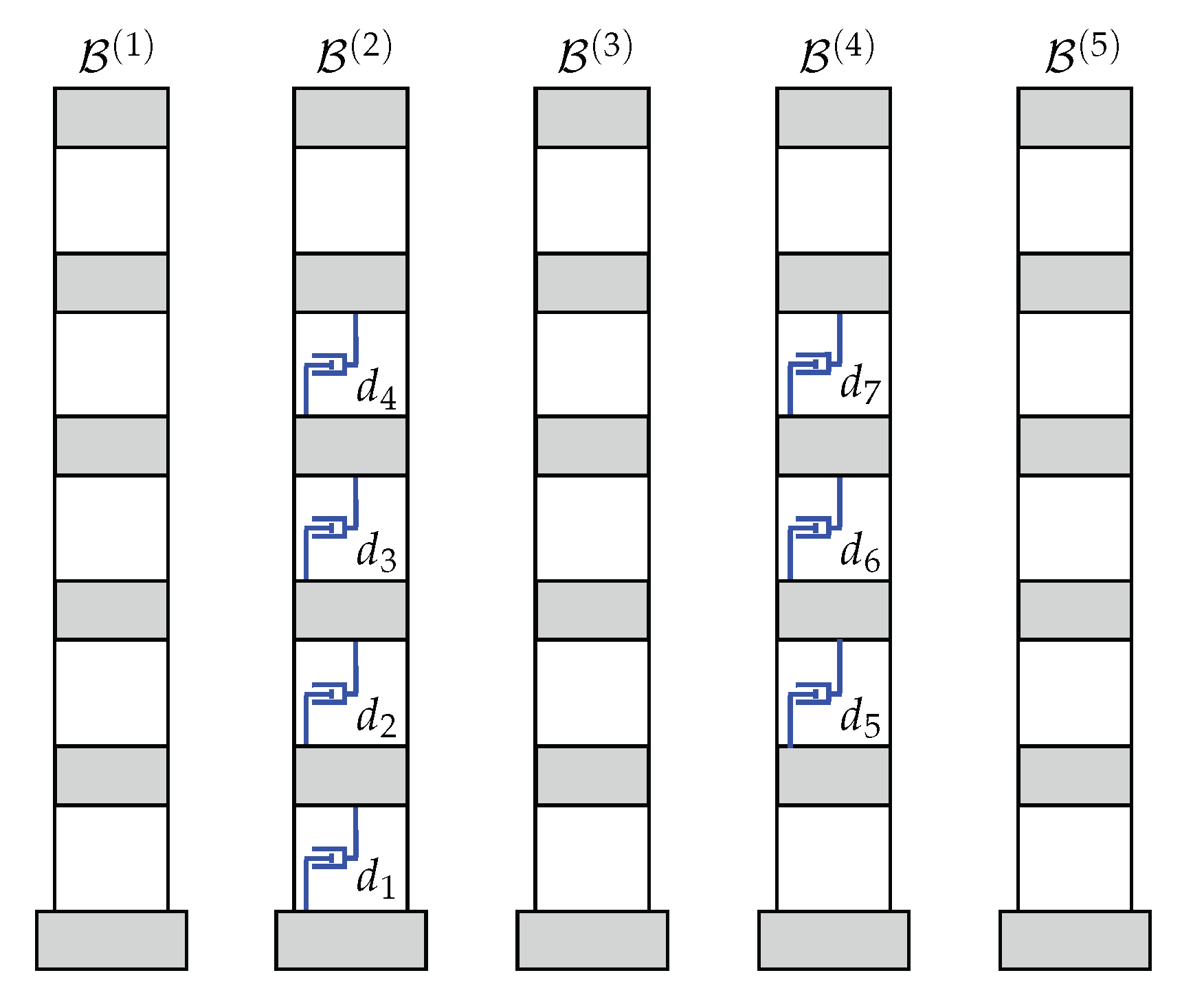
which corresponds to the system of interstory and interbuilding dampers displayed as blue and red small dashpots in Figure 5, respectively, and the damping coefficients collected in the first row of

Table 1. Values of the damping coefficients corresponding to the linked damping configurations DC1, DC2 and DC3 ($\times {10}^7$ Ns/m).

Conf.	${\mathit{d}}_1$	${\mathit{d}}_2$	${\mathit{d}}_3$	${\mathit{d}}_4$	${\mathit{d}}_5$	${\mathit{d}}_6$	${\mathit{d}}_7$	${\mathit{d}}_8$	${\mathit{d}}_9$	${\mathit{d}}_{10}$	${\mathit{d}}_{11}$	${\mathit{d}}_{12}$
DC1	1.4480	1.5137	1.3414	2.0098	2.1014	1.9725	1.5460	1.3074	0.4334	0.3683	0.8023	0.1528
DC2	1.8626	1.9882	1.7986	1.6611	2.1895	1.9489	1.6484	0.6311	0.4362	0.1519	0.0006	0.6828
DC3	2.6792	2.7151	2.5843	2.1407	0.2790	0.9873	0.7835	0.0009	1.3963	0.9310	0.0007	0.5018

.

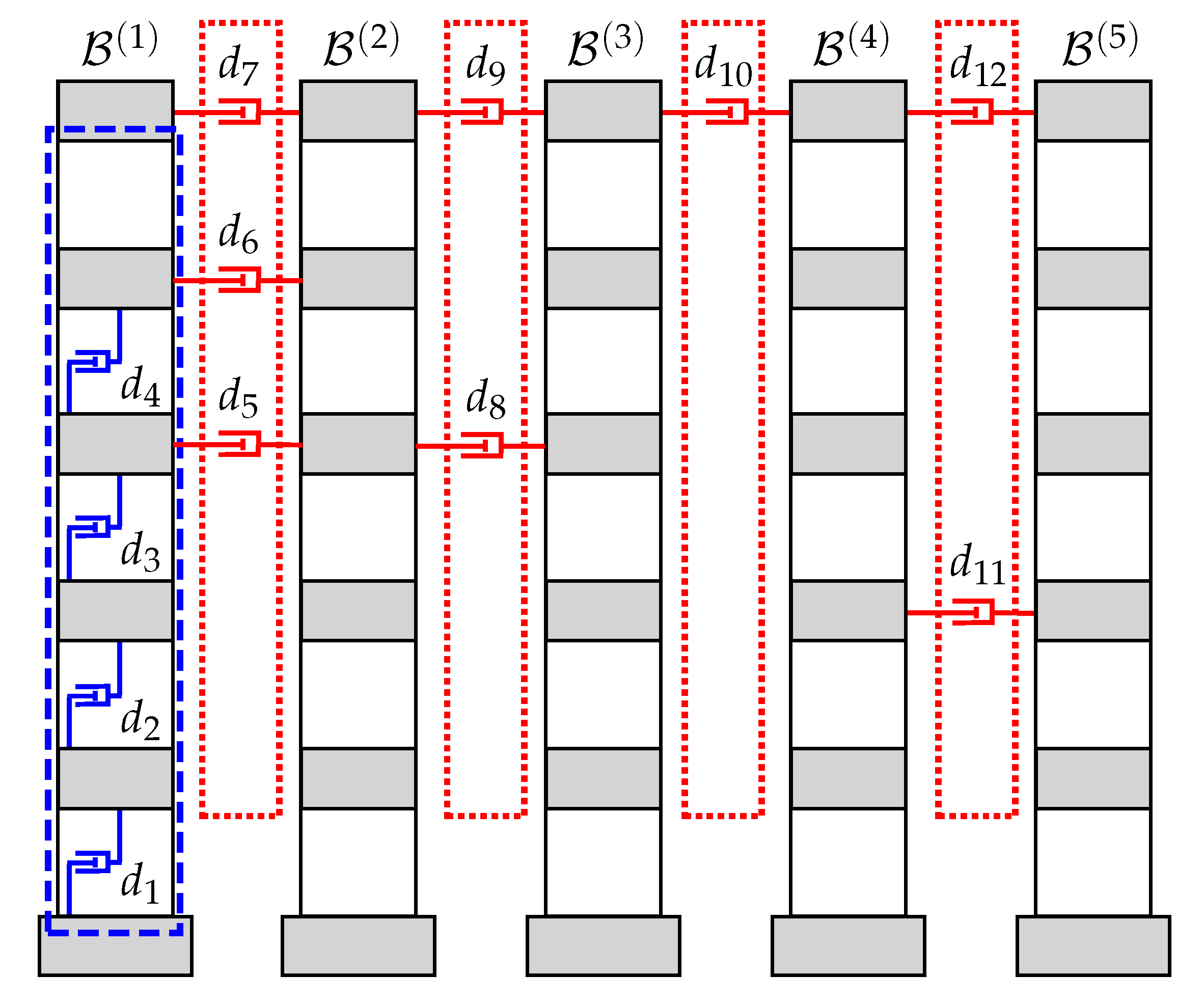
The second damping configuration (DC2), schematically displayed in Figure 6, allows placing dampers in the interstory positions

$${\widehat{\sigma }}^{\left(1\right)}=\left[\right],{\widehat{\sigma }}^{\left(2\right)}=[1,2,3,4,5],{\widehat{\sigma }}^{\left(3\right)}=\left[\right],{\widehat{\sigma }}^{\left(4\right)}=[1,2,3,4,5],{\widehat{\sigma }}^{\left(5\right)}=\left[\right]$$

(74)

and the interbuilding positions

$${\tilde{\sigma }}^{\left(1\right)}=[3,4,5],{\tilde{\sigma }}^{\left(2\right)}=[3,4,5],{\tilde{\sigma }}^{\left(3\right)}=[3,4,5],{\tilde{\sigma }}^{\left(4\right)}=[3,4,5],$$

(75)

which constrains the placement of interstory dampers to buildings ${\mathcal{B}}^{\left(2\right)}$ and ${\mathcal{B}}^{\left(4\right)}$ and restricts the placements of interbuilding dampers to the upper three interbuilding levels. In this second case, the total number of optimization variables is reduced to 34, with $\overline{\eta }=22$ binary allocation variables and $n_d=12$ continuous damping-coefficient variables. The optimal solution attained by the GA solver for DC2 includes the allocation list

$$\overline{\alpha }=[\stackrel{{\widehat{\alpha }}^{\left(2\right)}}{\overbrace{1,1,1,1,0}},\stackrel{{\widehat{\alpha }}^{\left(4\right)}}{\overbrace{0,1,1,1,0}},\stackrel{{\tilde{\alpha }}^{\left(1\right)}}{\overbrace{0,0,1}},\stackrel{{\tilde{\alpha }}^{\left(2\right)}}{\overbrace{0,0,1}},\stackrel{{\tilde{\alpha }}^{\left(3\right)}}{\overbrace{0,0,1}},\stackrel{{\tilde{\alpha }}^{\left(4\right)}}{\overbrace{1,1,0}}],$$

(76)

and the damping coefficients presented in the second row of Table 1.

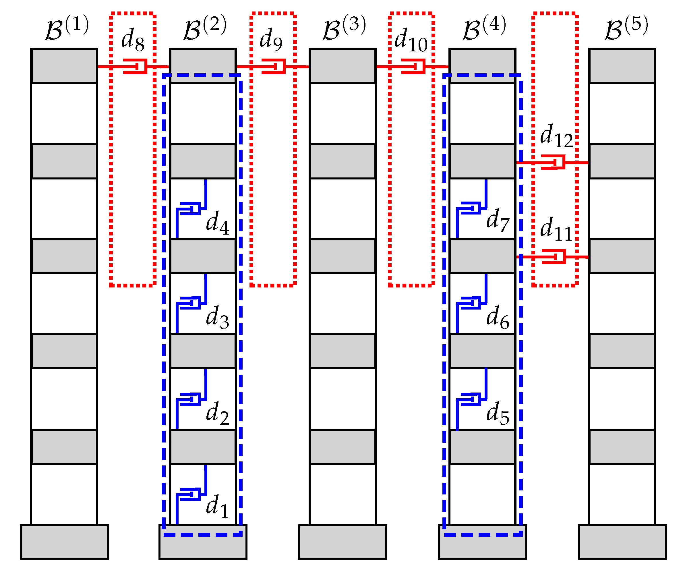
Finally, we consider the third damping configuration (DC3) displayed in Figure 7, which allows placing interbuilding dampers at all interbuilding positions and restricts interstory damper implementation to building ${\mathcal{B}}^{\left(1\right)}$. For that case, the schemes of allowed interstory and interbuilding damping positions are

$${\widehat{\sigma }}^{\left(1\right)}=[1,2,3,4,5],{\widehat{\sigma }}^{\left(2\right)}=\left[\right],{\widehat{\sigma }}^{\left(3\right)}=\left[\right],{\widehat{\sigma }}^{\left(4\right)}=\left[\right],{\widehat{\sigma }}^{\left(5\right)}=\left[\right]$$

(77)

and

$${\tilde{\sigma }}^{\left(1\right)}=[1,2,3,4,5],{\tilde{\sigma }}^{\left(2\right)}=[1,2,3,4,5],{\tilde{\sigma }}^{\left(3\right)}=[1,2,3,4,5],{\tilde{\sigma }}^{\left(4\right)}=[1,2,3,4,5],$$

(78)

respectively, and the total number of optimization variables is 37 with $\overline{\eta }=25$ binary damper-allocation variables and $n_d=12$ continuous damping-coefficient variables. The optimal allocation list obtained for DC3 is

$$\overline{\alpha }=[\stackrel{{\widehat{\alpha }}^{\left(1\right)}}{\overbrace{1,1,1,1,0}},\stackrel{{\tilde{\alpha }}^{\left(1\right)}}{\overbrace{0,0,1,1,1}},\stackrel{{\tilde{\alpha }}^{\left(2\right)}}{\overbrace{0,0,1,0,1}},\stackrel{{\tilde{\alpha }}^{\left(3\right)}}{\overbrace{0,0,0,0,1}},\stackrel{{\tilde{\alpha }}^{\left(4\right)}}{\overbrace{0,1,0,0,1}}],$$

(79)

and the corresponding damping coefficients are collected in the third row of Table 1.

Looking at the damping coefficient values in Table 1 and the structure of the optimal damper placements in Figure 5, Figure 6 and Figure 7, the following facts can be observed: (i) damping coefficients of interbuilding dampers are about one order of magnitude lower than those obtained for interstory dampers, (ii) interstory dampers tend to be placed in low building levels, and (iii) interbuilding dampers are preferably allocated at upper interbuilding positions. These facts are consistent with the results obtained in preliminary works on DDSs for MBSs [22,23]. It can also be observed in Table 1 that there are some dampers with particularly small damping coefficients. Specifically, damping coefficients $d_{11}$ in DC2 and $d_8$ and $d_{11}$ in DC3 are remarkably small when compared with the coefficient values of all the other interstory and interbuilding dampers. It should be noted that those small coefficients correspond to dampers placed at particularly low interbuilding positions and can be interpreted as a numerical side-effect of constraining the overall number of dampers to exactly $n_d=12$ elements. From a practical point of view, those residual dampers can be removed without any significant loss of performance and, consequently, the DDSs corresponding to the optimal configurations DC2 and DC3 could be implemented with a set of 11 and 10 dampers, respectively. Regarding the optimal $\gamma$-values, the data in

Table 2. Computational design characteristics of the linked DDS configurations DC1, DC2 and DC3.

Conf.	Act. Build.	${\mathit{H}}_{\mathit{\infty }}$ Norm	opt. vars.	Generations	funct. aval.	Time (s)	Parallel Time (s)
Plain conf.	—	0.8090	—	—	—	—	—
DC1	1, 3, 5	0.0897	47	206	41,400	273.5	167.9
DC2	2, 4	0.0970	34	161	32,400	242.8	157.5
DC3	1	0.1457	37	288	57,800	409.0	103.8

indicate that the considered damping configurations are all able to produce a significant reduction of the system $H_{\infty }$-norm when compared with the nonactuated MBS. In particular, an $H_{\infty }$-norm decrease around 82% is attained by DC3 and larger reductions of about 88% are achieved by DC1 and DC2. The better results obtained by DC1 and DC2 suggest a superior performance of widely distributed interstory damping schemes. However, it is worth highlighting the potential implementation advantages of DC3, which would only require internal modifications of building ${\mathcal{B}}^{\left(1\right)}$. As to the computational aspects, the selected GA solver has shown to be very effective in dealing with the mixture of discrete and continuous variables, the variety of optimization constraints and the relatively large number of optimization variables. All the presented damping configurations have been obtained with a common random seed and using the standard parameter setting for large-scale GA optimization problems suggested in the Matlab Global Optimization Toolbox. Considering the dimension and complexity of the problem and the modest computing resources (see Remark 8), the computation times are notably short, specially when the GA solver is run in parallel mode. Finally, the large number of objective-function evaluations required to obtain the different optimal configurations indicates that the computational cost of evaluating the objective function can certainly be a critical bottleneck for the overall computational effectiveness of the proposed design methodology. In that sense, the presented matrix formulation for the damped multibuilding model has proved to be a relevant contribution.

Remark 6.

As suggested in the GA solver documentation for problems with a large number of optimization variables [31], we have introduced some modifications in the default parameter setting of the solver. Specifically, we have set the values 200 for thePopulationSize, 0.9 for theCrossoverFraction, 20 for theEliteCountand 500 for theMaxGenerationsparameters. To take advantage of the CPU multi-core architecture, the GA solver has been enforced to run in parallel mode by enabling the optionUseParallel. Also, to improve the relative accuracy in the computation of the $H_{\infty }$-norm, the tolerance in the functionhinfnormhas been decreased to ${10}^{-3}$ [30].

Remark 7.

As indicated in Remark 5, the stochastic character of the GA solver typically produces distinct suboptimal solutions in different runs of the solver. For simplicity, in this work the Matlab orderrng(125)has been used to set a common random seed for all the computed DDS configurations. That random seed has been arbitrarily chosen, which confirms the effectiveness of the proposed design methodology and indicates that improved results could be possibly obtained by exploring a wider set of random seeds [29].

Remark 8.

The computation time values presented in Table 2 should only be taken as approximate references, in the sense that small variations can be observed in the computation time of different runs of the GA solver. Moreover, the computation time in parallel mode can be significantly affected by the available number of CPU cores. In this work, all the computations have been carried out with Matlab 2019a on a regular desktop computer equipped with an Intel Core i7-8700 CPU at 3.20 GHz, 16 GB RAM and a 480GB SSD hard drive.

5. Seismic Responses

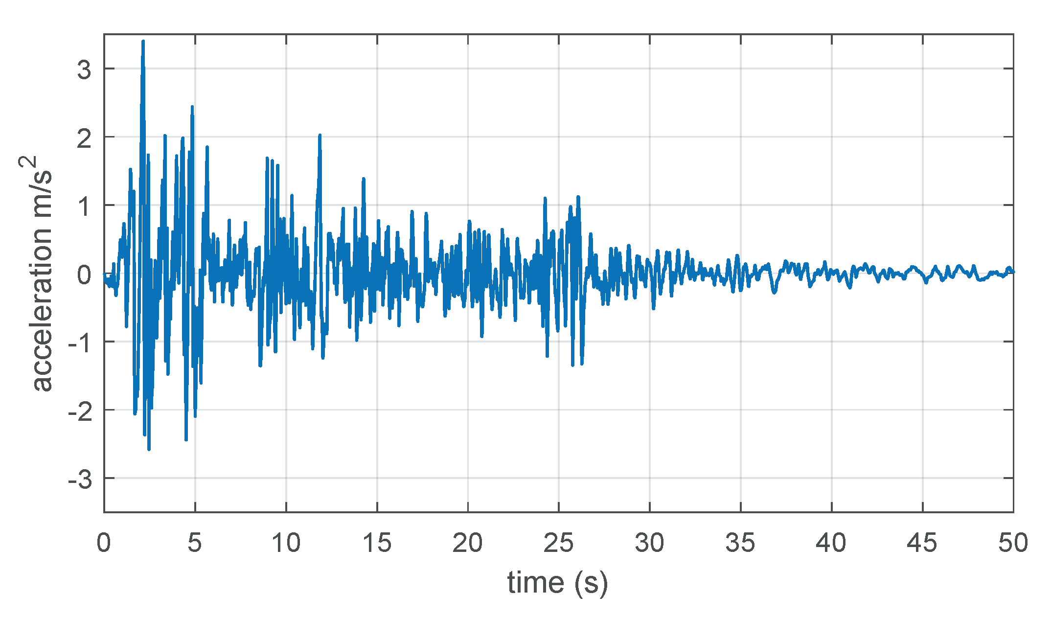
To illustrate the behavior of the different DDSs designed in Section 4, we have carried out a proper set of numerical simulations using the full-scale 180-component of El Centro 1940 seismic record as ground acceleration disturbance (see Figure 8). Specifically, for the nonactuated MBS and the damping configurations DC1, DC2 and DC3, we have computed the maximum absolute interstory drifts

$$|{\widehat{r}}_i^j{|}_{\max }=\underset{0\le t\le T_w}{max}\left|{\widehat{r}}_i^j\left(t\right)\right|,i=1,\dots ,5,j=1,\dots ,5,$$

(80)

the maximum absolute story total-accelerations

$$|a_i^j{|}_{\max }=\underset{0\le t\le T_w}{max}\left|a_i^j\left(t\right)\right|,i=1,\dots ,5,j=1,\dots ,5$$

(81)

and the maximum interbuilding approachings

$${({\tilde{r}}_i^j)}_{\max }=\underset{0\le t\le T_w}{max}{\tilde{r}}_i^j\left(t\right),i=1,\dots ,5,j=1,\dots ,4,$$

(82)

where ${\widehat{r}}_i^j\left(t\right)$, $a_i^j\left(t\right)$ and ${\tilde{r}}_i^j\left(t\right)$ are the output variables defined in Equations (33), (37) and (40), respectively, and $T_w$ denotes the total duration of the seismic disturbance.

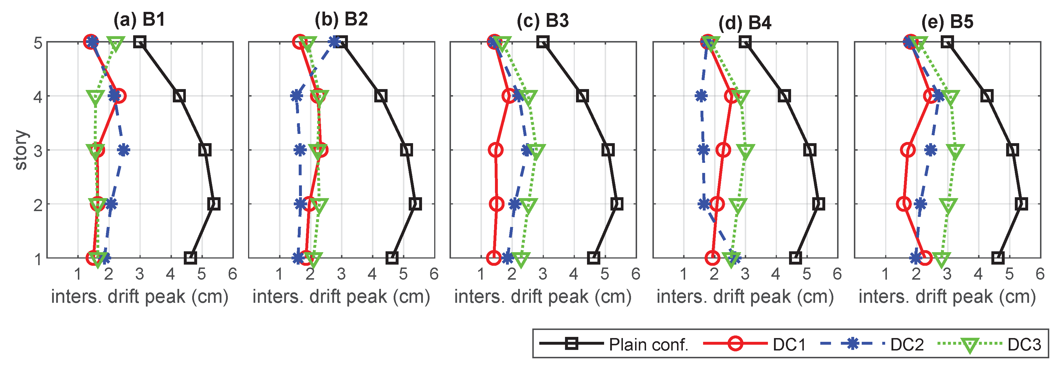
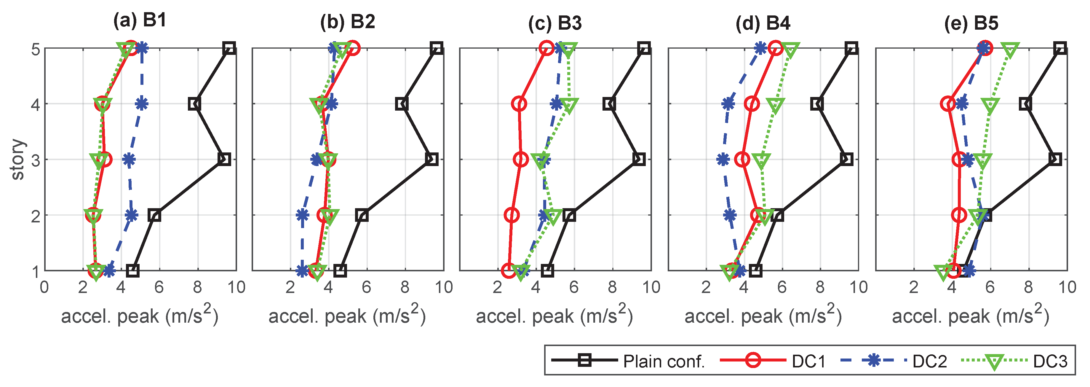
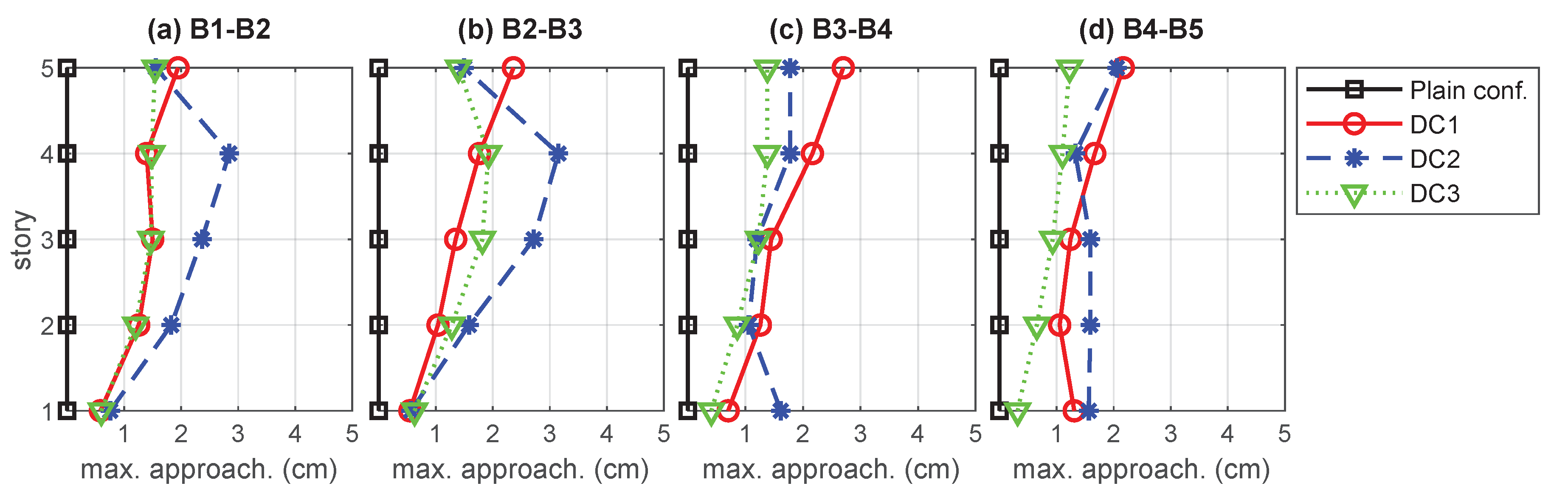
The obtained interstory-drift peak-values are presented in Figure 9. A global view of the plots in that figure indicates that the three designed damping configurations are all able to produce an overall reduction of the interstory-drift peak-values when compared with the response of the nonactuated MBS (black solid lines with rectangles). In a more detailed inspection of the DC1 response (red solid lines with circles), it can be appreciated that the interstory-drift peak-value reduction is particularly effective in the actuated buildings ${\mathcal{B}}^{\left(1\right)}$, ${\mathcal{B}}^{\left(3\right)}$ and ${\mathcal{B}}^{\left(5\right)}$. A slightly poorer performance can be observed in the nonactuated buildings ${\mathcal{B}}^{\left(2\right)}$ and ${\mathcal{B}}^{\left(4\right)}$, whose seismic protection is provided through the linking interbuilding dampers (see Figure 5). A similar behavior can be observed in the response of the damping configuration DC2 (blue dashed lines with asterisks), where ${\mathcal{B}}^{\left(2\right)}$ and ${\mathcal{B}}^{\left(4\right)}$ are actuated buildings and ${\mathcal{B}}^{\left(1\right)}$, ${\mathcal{B}}^{\left(3\right)}$ and ${\mathcal{B}}^{\left(5\right)}$ are nonactuated (see Figure 6). In this case, it is worth noting the loss of performance in the upper level of building ${\mathcal{B}}^{\left(2\right)}$, which is an effect that has been observed in previous works [22] and can be associated to the action of the interbuilding links. Finally, for the single-actuated-building configuration DC3 (green dotted lines with triangles), the best results are also attained in the actuated building ${\mathcal{B}}^{\left(1\right)}$, and a moderate but gradual increase of the interstory-drift peak-values can be observed in the nonactuated buildings as we move away from ${\mathcal{B}}^{\left(1\right)}$. Also in this case, a loss of performance associated to the interbuilding links can be appreciated in the upper level of the actuated building ${\mathcal{B}}^{\left(1\right)}$. The obtained story total-acceleration peak-values and maximum interbuilding approachings are displayed in Figure 10 and Figure 11, respectively, using the same colors, line styles and symbols. The plots in Figure 10 confirm that, despite having only included the interstory drifts in the optimization index, the considered $H_{\infty }$ design approach can produce a notable reduction of the acceleration peak-values. That reduction is more relevant in the actuated buildings and smaller but yet significant in the nonactuated ones. Also in this case, it can be appreciated the progressive loss of performance of the configuration DC3 as we move away from the only actuated building ${\mathcal{B}}^{\left(1\right)}$. Regarding the approaching peak-values, the plots in Figure 11 show that the three damping configurations are able to keep the interbuilding approachings within remarkably low levels. In fact, for the considered seismic disturbance, an interbuilding gap of 3.5 cm can be considered a safe interbuilding separation in all the cases. It is worth noting that the best approaching results are attained by the single-actuated-building configuration DC3, which can be explained by the stronger interbuilding damping system of that configuration.

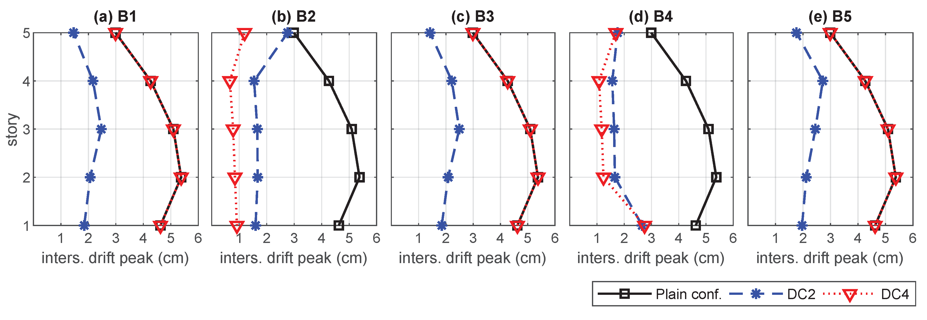
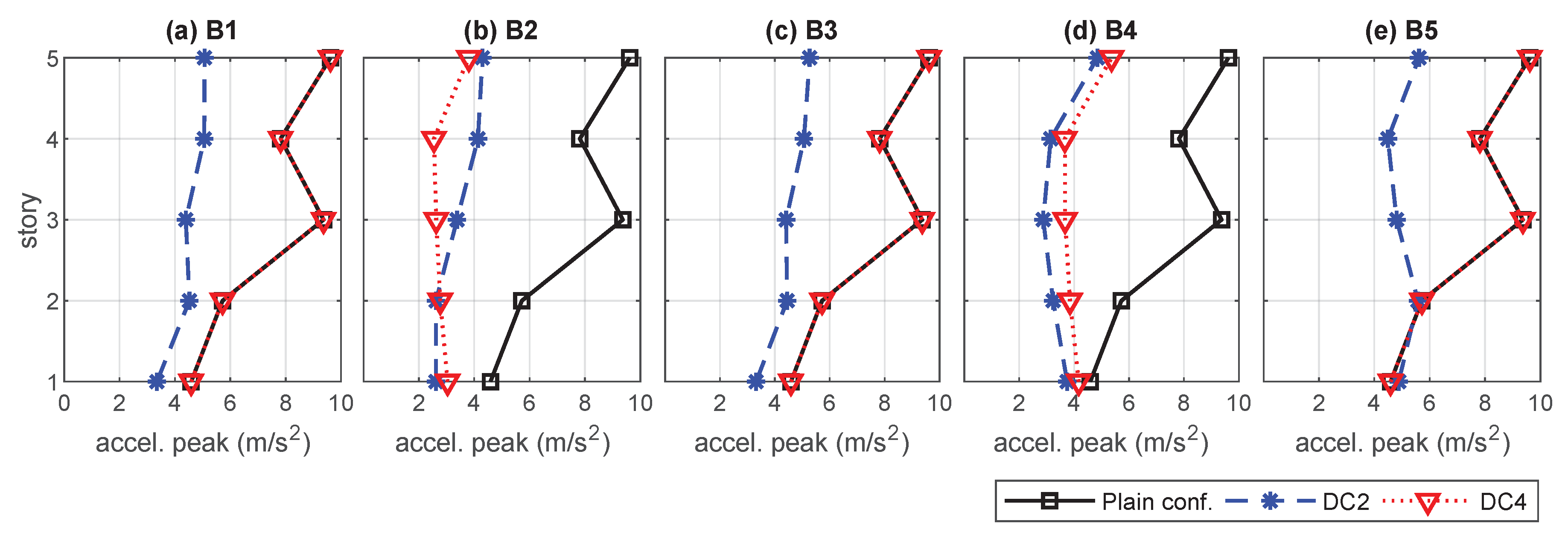
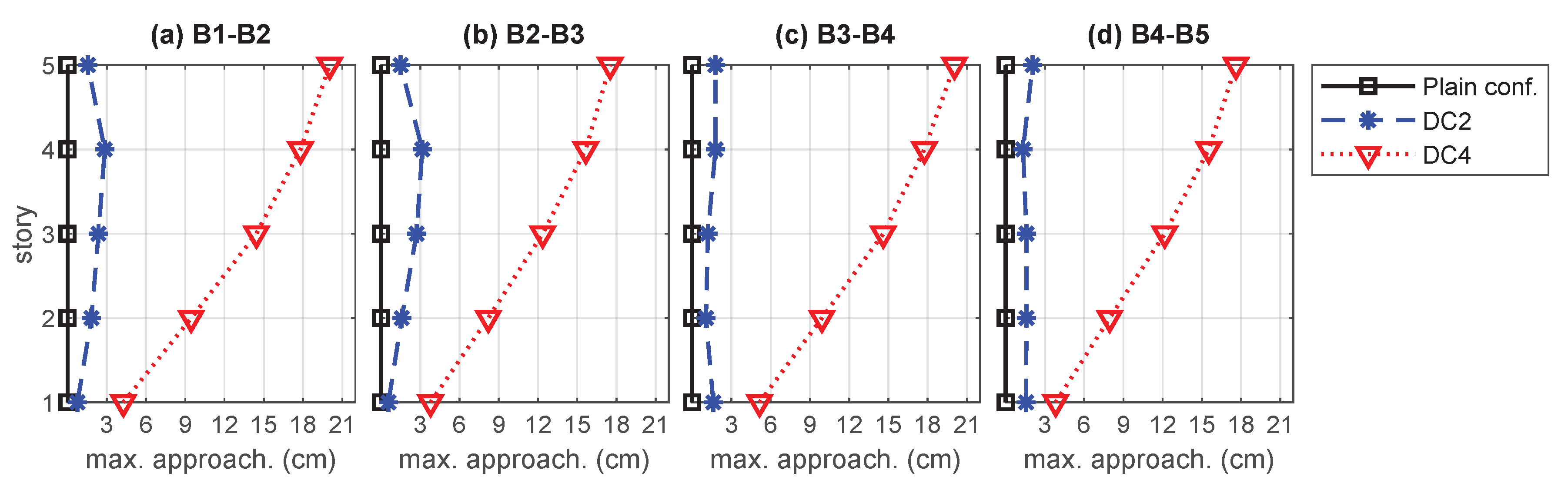
To gain a better understanding of the relevance of linked configurations in the seismic protection of the overall MBS, we have considered an additional unlinked damping configuration DC4 (see Figure 12), which has been obtained by removing the interbuilding dampers in the linked configuration DC2. The interstory-drift and acceleration peak-values produced by DC4 are displayed in Figure 13 and Figure 14, respectively, and the corresponding maximum approachings are presented in Figure 15. The peak-values produced by the nonactuated MBS and the linked configuration DC2 are also included in those figures as a reference. Looking at the plots of interstory-drift peak-values in Figure 13, it can be appreciated that the unlinked configuration DC4 (red dotted lines with triangles) produces better results than the linked configuration DC2 in the actuated buildings ${\mathcal{B}}^{\left(2\right)}$ and ${\mathcal{B}}^{\left(4\right)}$, but it provides null protection to the nonactuated buildings ${\mathcal{B}}^{\left(1\right)}$, ${\mathcal{B}}^{\left(3\right)}$ and ${\mathcal{B}}^{\left(5\right)}$. The plots of acceleration peak-values in Figure 14 indicate that, in addition of providing null protection to the nonactuated buildings, the unlinked configuration DC4 attains worse results than the linked configuration DC2 in building ${\mathcal{B}}^{\left(4\right)}$ and the first story of building ${\mathcal{B}}^{\left(2\right)}$. As to the interbuilding approachings, the plots in Figure 15 show that large approaching peak-values are produced at the top level of all the buildings by the unlinked configuration DC4, which would require interbuilding separations of about 20 cm to avoid pounding.

Finally, to summarize the global behavior of the nonactuated MBS and the discussed damping configurations, we consider the overall peak-values of absolute interstory drifts

$$|\widehat{r}{|}_{\max }=\underset{1\le j\le m}{max}\left(\underset{1\le i\le n}{max}{\left|{\widehat{r}}_i^j\right|}_{\max }\right),$$

(83)

absolute story total-accelerations

$${\left|a\right|}_{\max }=\underset{1\le j\le m}{max}\left(\underset{1\le i\le n}{max}{\left|a_i^j\right|}_{\max }\right)$$

(84)

and interbuilding approachings

$${\left(\tilde{r}\right)}_{\max }=\underset{1\le j\le m-1}{max}\left(\underset{1\le i\le n}{max}{({\tilde{r}}_i^j)}_{\max }\right).$$

(85)

The obtained overall peak-values and the corresponding $H_{\infty }$-norms are collected in

Table 3. $H_{\infty }$ norm and overall maximum peak-values corresponding to the nonactuated multibuilding system (plain configuration), the linked configurations DC1, DC2 and DC3, and the unlinked configuration DC4.

Conf.	Act. Build.	${\mathit{H}}_{\mathit{\infty }}$ Norm	Max. drift (cm)	Max. accel. (m/s${}^2$)	Max. Approach. (cm)
Plain	—	0.8090	5.38	9.62	20.00
DC1	1, 3, 5	0.0897	2.56	5.71	22.70
DC2	2, 4	0.0970	2.76	5.62	23.15
DC3	1	0.1457	3.25	7.02	21.92
DC4	2, 4	0.6272	5.38	9.62	20.05

. The data in the table indicate that, with respect to the nonactuated MBS, the DDS configurations DC1 and DC2 produce reductions of about 50% in the overall interstory-drift peak-value and around 40% in the overall acceleration peak-value. The overall reductions attained by the single-actuated-building configuration DC3 are around 40% in the interstory-drift and slightly below 30% in the acceleration responses. The overall maximum approaches are around 3 cm for DC1 and DC2 and inferior to 2 cm for DC3. Those values indicate that the linked DDSs obtained with the proposed design strategy can provide an overall seismic protection for the MBS. At the same time, the values corresponding to DC4 illustrate the inefficacy of unlinked configurations in mitigating the interstory-drift and acceleration seismic response of the overall MBS and clearly demonstrate their possible detrimental effects on pounding risk.

Remark 9.

The plots in Figure 15 indicate that null interbuilding approachings are produced by the nonactuated MBS, which can be explained by the synchronized response of the identical buildings subjected to the same seismic excitation. From a practical point of view, however, it should be observed that there are a number of factors, such as the differential variation of the building structural parameters over time, the effect of live loads (weight of persons, furniture, equipment, movable partitions, etc.) or the soil-structure interaction, that can brake the ideal synchrony of the buildings response and, consequently, increase the risk of pounding.

6. Conclusions

In this work, we have investigated the design of distributed damping systems (DDSs) for the overall seismic protection of multiple adjacent buildings. The considered DDSs include two different kinds of damping devices: interstory dampers, which are implemented inside the buildings, and external interbuilding damping links. To keep the problem complexity within reasonable limits, we have assumed that the damping elements are linear fluid viscous dampers and the buildings have been considered as linear planar frames with identical dynamic characteristics. The main objective of the study is designing suitable DDS configurations that are able to mitigate the buildings seismic response by reducing the interstory-drift and story-acceleration peak-values and, at the same time, are capable of cutting down the risk of interbuilding collisions (pounding) by producing small interbuilding approachings. Typically, designing high-performance DDSs involves solving a mixed allocation-tuning optimization problem, which includes both determining convenient damper positions and computing proper values for the damper parameters. The proposed design methodology is based on an effective matrix formulation of the damped multibuilding system, follows an $H_{\infty }$ approach that permits avoiding costly numerical simulations of seismic time-responses, exploits the computational advantages of state-of-the-art genetic algorithm (GA) solvers, and allows setting actuation schemes of particular interest such as full-linked configurations or nonactuated buildings. To illustrate the main features of the presented design strategy, three different DDS configurations have been computed for a system of five adjacent multistory buildings. Also, to explore the performance characteristics of the obtained DDS configurations, a convenient set of numerical simulations of the corresponding seismic responses have been carried out using the full-scale 180-component of El Centro 1940 seismic record as ground acceleration input. Considering the obtained results, the following points can be highlighted: (i) properly designed DDSs can provide an overall seismic protection to systems of multiple adjacent buildings, being able to mitigate the buildings seismic response and reduce the pounding risk; (ii) full-linked DDS configurations should be used to attain the seismic protection of nonactuated buildings and to produce low levels of pounding risk; (iii) a simultaneous reduction of the buildings interstory-drift and story-accelerations peak values can be attained with the considered $H_{\infty }$ approach; (iv) the proposed design methodology is highly flexible, being able to produce high-performance DDS configurations for a wide variety of actuation schemes; and (v) the proposed approach is computationally effective in dealing with large-scale problems. Regarding that last point, it should be observed that computational efficiency is a critical factor in DDS design of multibuilding problems. In this context, a fast evaluation of the objective function and the possibility of running the GA solver in parallel mode are elements of singular relevance.

After the positive results obtained in the present work, we believe that further research effort should be invested in obtaining a deeper understanding of the problem and removing some of the model simplifications introduced in this paper. In that sense, some lines of particular interest include the usage of inerter-based vibration absorbers [36,37], the study of the effects of interstory and interbuilding velocities on the multibulding damper allocation problem [38,39], the analysis of the effects produced by soil-structure interaction [40] and seismic-wave propagation [41] on large multibulding problems, and the formulation of extended design strategies for elastic-plastic structures [42] and/or nonlinear damping devices [43].

References

- Soong, T.T.; Spencer, B.F., Jr. Supplemental energy dissipation: state-of-the-art and state-of-the-practice. Eng. Struct. 2002, 24, 243–259. [Google Scholar] [CrossRef]
- Ali, M.M.; Moon, K.S. Structural developments in tall buildings: Current trends and future prospects. Archit. Sci. Rev. 2007, 50, 205–223. [Google Scholar] [CrossRef]
- Takewaki, I.; Fujita, K.; Yamamoto, K.; Takabatake, H. Smart passive damper control for greater building earthquake resilience in sustainable cities. Sustain. Cities Soc. 2011, 1, 3–15. [Google Scholar] [CrossRef] [Green Version]
- Wang, S.; Mahin, S.A. Seismic retrofit of a high-rise steel moment-resisting frame using fluid viscous dampers. Struct. Des. Tall Special Build. 2017, 26, 1–11. [Google Scholar] [CrossRef]
- Aydin, E.; Ozturk, B.; Dutkiewicz, M. Analysis of efficiency of passive dampers in multistorey buildings. J. Sound Vib. 2019, 439, 17–28. [Google Scholar] [CrossRef]
- Li, Z.; Shu, G.; Huang, Z. Proper configuration of metallic energy dissipation system in shear-type building structures subject to seismic excitation. J. Constr. Steel Res. 2019, 154, 177–189. [Google Scholar] [CrossRef]
- De Domenico, D.; Ricciardi, G.; Takewaki, I. Design strategies of viscous dampers for seismic protection of building structures: A review. Soil Dyn. Earthq. Eng. 2019, 118, 144–165. [Google Scholar] [CrossRef]
- López García, D.; Soong, T.T. Efficiency of a simple approach to damper allocation in MDOF structures. J. Struct. Control 2002, 9, 19–30. [Google Scholar] [CrossRef]
- Liu, W.; Tong, M.; Lee, G.C. Optimization methodology for damper configuration based on building performance indices. J. Struct. Eng. 2005, 131, 1746–1756. [Google Scholar] [CrossRef]
- Main, J.A.; Krenk, S. Efficiency and tuning of viscous dampers on discrete systems. J. Sound Vib. 2005, 286, 97–122. [Google Scholar] [CrossRef]
- Fujita, K.; Yamamoto, K.; Takewaki, I. An evolutionary algorithm for optimal damper placement to minimize interstorey-drift transfer function in shear building. Earthq. Struct. 2010, 1, 289–306. [Google Scholar] [CrossRef]
- Del Gobbo, G.M.; Williams, M.S.; Blakeborough, A. Comparing fluid viscous damper placement methods considering total-building seismic performance. Earthq. Eng. Struct. Dyn. 2018, 47, 2864–2886. [Google Scholar] [CrossRef]
- Singh, M.P.; Moreschi, L.M. Optimal seismic response control with dampers. Earthq. Eng. Struct. Dyn. 2001, 30, 553–572. [Google Scholar] [CrossRef]
- Huang, X. Evaluation of genetic algorithms for the optimum distribution of viscous dampers in steel frames under strong earthquakes. Earthq. Struct. 2018, 14, 215–227. [Google Scholar]
- Cetin, H.; Aydin, E.; Ozturk, B. Optimal design and distribution of viscous dampers for shear building structures under seismic excitations. Front. Built Environ. 2019, 5, 1–13. [Google Scholar] [CrossRef] [Green Version]
- Del Gobbo, G.M. Placement of fluid viscous dampers to improve total-building seismic performance. In Proceedings of the CSCE Annual Conference, Laval, Montreal, QC, Canada, 12–15 June 2019; pp. 1–9. [Google Scholar]
- Tubaldi, E. Dynamic behavior of adjacent buildings connected by linear viscous/viscoelastic dampers. Struct. Control Health Monit. 2015, 22, 1086–1102. [Google Scholar] [CrossRef]
- Kandemir-Mazanoglu, E.C.; Mazanoglu, K. An optimization study for viscous dampers between adjacent buildings. Mech. Syst. Signal Process. 2017, 89, 88–96. [Google Scholar] [CrossRef]
- Liu, M.Y.; Wang, A.P.; Chiu, M.Y. Optimal vibration control of adjacent building structures interconnected by viscoelastic dampers. J. Civ. Eng. Arch. 2017, 11, 468–476. [Google Scholar]
- Patel, C.C. Dynamic response of viscous damper connected similar multi-degree of freedom structures. Int. J. Earth Sci. Eng. 2011, 4, 1068–1071. [Google Scholar]
- Patel, C.C.; Jangid, R.S. Dynamic response of identical adjacent structures connected by viscous damper. Struct. Control Health Monit. 2014, 21, 205–224. [Google Scholar] [CrossRef]
- Palacios-Quiñonero, F.; Rubió-Massegú, J.; Rossell, J.M.; Karimi, H.R. Integrated design of hybrid interstory-interbuilding multi-actuation schemes for vibration control of adjacent buildings under seismic excitations. Appl. Sci. 2017, 7, 323. [Google Scholar] [CrossRef] [Green Version]
- Palacios-Quiñonero, F.; Rubió-Massegú, J.; Rossell, J.; Rodellar, J. Interstory-interbuilding actuation schemes for seismic protection of adjacent identical buildings. Smart Struct. Syst. 2019, 24, 67–81. [Google Scholar]
- Del Gobbo, G.M.; Blakeborough, A.; Williams, M.S. Improving total-building seismic performance using linear fluid viscous dampers. Bull. Earthq. Eng. 2018, 16, 4249–4272. [Google Scholar] [CrossRef] [Green Version]
- Yang, J.N.; Lin, S.; Kim, J.-H.; Agrawal, A.K. Optimal design of passive energy dissipation systems based on H∞ and H2 performances. Earthq. Eng. Struct. Dyn. 2002, 31, 921–936. [Google Scholar] [CrossRef]
- Palacios-Quiñonero, F.; Rubió-Massegú, J.; Rossell, J.M.; Karimi, H.R. Optimal passive-damping design using a decentralized velocity-feedback H∞ approach. Model. Identif. Control 2012, 33, 87–97. [Google Scholar] [CrossRef] [Green Version]
- Abdeddaim, M.; Ounis, A.; Djedoui, N.; Shrimali, M.K. Pounding hazard mitigation between adjacent planar buildings using coupling strategy. J. Civ. Struct. Health Monit. 2016, 6, 603–617. [Google Scholar] [CrossRef]
- Jankowski, R.; Mahmoud, S. Linking of adjacent three-storey buildings for mitigation of structural pounding during earthquakes. Bull. Earthq. Eng. 2016, 14, 3075–3097. [Google Scholar] [CrossRef] [Green Version]
- Palacios-Quiñonero, F.; Rubió-Massegú, J.; Rossell, J.M.; Karimi, H.R. Design of inerter-based multi-actuator systems for vibration control of adjacent structures. J. Frankl. Inst. 2019, 356, 7785–7809. [Google Scholar]
- Balas, G.J.; Chiang, R.Y.; Packard, A.K.; Safonov, M.G. MATLAB Robust Control Toolbox User’s Guide, 2019a; The MathWorks, Inc.: Natick, MA, USA, 2019. [Google Scholar]
- MathWorks. MATLAB Global Optimization Toolbox User’s Guide, 2019a; The MathWorks, Inc.: Natick, MA, USA, 2019. [Google Scholar]
- Chopra, A. Dynamics of Structures. Theory and Applications to Earthquake Engineering, 3rd ed.; Prentice Hall: Upper Saddle River, NJ, USA, 2007. [Google Scholar]
- Wang, Y.; Lynch, J.P.; Law, K.H. Decentralized H∞ controller design for large-scale civil structures. Earthq. Eng. Struct. Dyn. 2009, 38, 377–401. [Google Scholar] [CrossRef]
- MathWorks. MATLAB Control System Toolbox User’s Guide, 2019a; The MathsWorks, Inc.: Natick, MA, USA, 2019. [Google Scholar]
- Kurata, N.; Kobori, T.; Takahashi, M.; Niwa, N.; Midorikawa, H. Actual seismic response controlled building with semi-active damper system. Earthq. Eng. Struct. Dyn. 1999, 28, 1427–1447. [Google Scholar] [CrossRef]
- Wang, Q.; Qiao, H.; De Domenico, D.; Zhu, Z.; Xie, Z. Wind-induced response control of high-rise buildings using inerter-based vibration absorbers. Appl. Sci. 2019, 9, 5045. [Google Scholar] [CrossRef]
- Petrini, F.; Giaralis, A.; Wang, Z. Optimal tuned mass-damper-inerter (TMDI) design in wind-excited tall buildings for occupants’ comfort serviceability performance and energy harvesting. Eng. Struct. 2020, 204, 1–16. [Google Scholar] [CrossRef]
- Adachi, F.; Fujita, K.; Tsuji, M.; Takewaki, I. Importance of interstory velocity on optimal along-height allocation of viscous oil dampers in super high-rise buildings. Eng. Struct. 2013, 56, 489–500. [Google Scholar] [CrossRef] [Green Version]
- Logotheti, V.E.; Kafetzi, T.C.; Papagiannopoulos, G.A.; Karabalis, L.K. On the use of interstorey velocity for the seismic retrofit of steel frames with viscous dampers. Soil Dyn. Earthq. Eng. 2020, 129, 1–14. [Google Scholar] [CrossRef]
- Sarcheshmehpour, M.; Estekanchi, H.E.; Ghannad, M.A. Optimum placement of supplementary viscous dampers for seismic rehabilitation of steel frames considering soil–structure interaction. Struct. Des. Tall Special Build. 2020, 29, 1–17. [Google Scholar] [CrossRef]
- Savor Novak, M.; Lazarevic, D.; Atalic, J.; Uros, M. Influence of multiple-support excitation on seismic response of reinforced concrete arch bridges. Appl. Sci. 2020, 10, 17. [Google Scholar] [CrossRef] [Green Version]
- Akehashi, H.; Takewaki, I. Optimal viscous damper placement for elastic-plastic MDOF structures under critical double impulse. Front. Built Environ. 2019, 5, 1–17. [Google Scholar] [CrossRef] [Green Version]
- De Domenico, D.; Ricciardi, G. Earthquake protection of structures with nonlinear viscous dampers optimized through an energy-based stochastic approach. Eng. Struct. 2019, 179, 523–539. [Google Scholar] [CrossRef]
Figure 1.
System of adjacent buildings equipped with a distributed set of interstory and interbuilding dampers.
Figure 2.
Schematic mechanical model of a five-story building equipped with a distributed system of supplemental interstory dampers implemented at the story levels , and .
Figure 3.
Interbuilding separation of the stories and corresponding to the interbuilding approaching for adjacent buildings and with an interbuilding gap .
Figure 4.
Schemes of allowed damper positions for a three-building system. Interstory scheme with , and (blue dashed rectangles). Interbuilding scheme with and (red dotted rectangles).
Figure 5.
Damping configuration DC1. Full-linked distributed damping system (DDS) with three actuated buildings, interstory dampers and interbuilding dampers.
Figure 6.
Damping configuration DC2. Full-linked DDS with two actuated buildings, interstory dampers and interbuilding dampers.
Figure 7.
Damping configuration DC3. Full-linked DDS with a single actuated building, interstory dampers and interbuilding dampers.
Figure 8.
Full-scale 180-component of El Centro 1940 ground-acceleration seismic record with an absolute acceleration-peak of 3.417 m/s. Data available at Strong-Motion Virtual Data Center (VDC) (ftp://strongmotioncenter.org/vdc/smdb/1940/c/139u37el.c0a).
Figure 9.
Maximum absolute interstory drifts corresponding to the nonactuated multibuilding system (plain configuration) and the damping configurations DC1, DC2 and DC3.
Figure 10.
Maximum absolute story total-accelerations attained by the nonactuated multibuilding system (plain configuration) and the damping configurations DC1, DC2 and DC3.
Figure 11.
Maximum interbuilding approachings produced by the nonactuated multibuilding system (plain configuration) and the damping configurations DC1, DC2 and DC3.
Figure 12.
Fully unlinked damping configuration DC4 obtained by suppressing the interbuilding dampers in the linked configuration DC2.
Figure 13.
Maximum absolute interstory drifts corresponding to the nonactuated multibuilding system (plain configuration), the linked configuration DC2 and the unlinked configuration DC4.
Figure 14.
Maximum absolute story total-accelerations attained by the nonactuated multibuilding system (plain configuration), the linked configuration DC2 and the unlinked configuration DC4.
Figure 15.
Maximum interbuilding approachings produced by the nonactuated multibuilding system (plain configuration), the linked configuration DC2 and the unlinked configuration DC4.