Article

Evaluation of Classical Mathematical Models of Tumor Growth Using an On-Lattice Agent-Based Monte Carlo Model †

by
Samuel Ruiz-Arrebola
1,
Damián Guirado
2,3,
Mercedes Villalobos
3,4,5 and
Antonio M. Lallena
3,6,*
1
Servicio de Oncología Radioterápica, Hospital Universitario Marqués de Valdecilla, E-39008 Santander, Spain
2
Unidad de Radiofísica, Hospital Universitario Clínico San Cecilio, E-18016 Granada, Spain
3
Instituto de Investigación Biosanitaria (ibs.GRANADA), Universidad de Granada, E-18016 Granada, Spain
4
Departamento de Radiología y Medicina Física, Universidad de Granada, E-18071 Granada, Spain
5
Instituto de Biopatología y Medicina Regenerativa (IBIMER), Universidad de Granada, E-18071 Granada, Spain
6
Departamento de Física Atómica, Molecular y Nuclear, Universidad de Granada, E-18071 Granada, Spain
*
Author to whom correspondence should be addressed.
This work is part of the Ph.D. thesis developed by S. Ruiz-Arrebola within the Ph.D. program “Clinical Medicine and Public Health” at the University of Granada, Spain.
Appl. Sci. 2021, 11(11), 5241; https://doi.org/10.3390/app11115241
Submission received: 2 April 2021 / Revised: 21 May 2021 / Accepted: 28 May 2021 / Published: 4 June 2021

Abstract

:

Featured Application

The analysis carried out has shown that the Gompertz model has the best predictive capabilities concerning the tumor growth. This model should substitute the exponential one in clinical practice.

Abstract

Purpose: To analyze the capabilities of different classical mathematical models to describe the growth of multicellular spheroids simulated with an on-lattice agent-based Monte Carlo model that has already been validated. Methods: The exponential, Gompertz, logistic, potential, and Bertalanffy models have been fitted in different situations to volume data generated with a Monte Carlo agent-based model that simulates the spheroid growth. Two samples of pseudo-data, obtained by assuming different variability in the simulation parameters, were considered. The mathematical models were fitted to the whole growth curves and also to parts of them, thus permitting to analyze the predictive power (both prospective and retrospective) of the models. Results: The consideration of the data obtained with a larger variability of the simulation parameters increases the width of the χ 2 distributions obtained in the fits. The Gompertz model provided the best fits to the whole growth curves, yielding an average value of the χ 2 per degree of freedom of 3.2, an order of magnitude smaller than those found for the other models. Gompertz and Bertalanffy models gave a similar retrospective prediction capability. In what refers to prospective prediction power, the Gompertz model showed by far the best performance. Conclusions: The classical mathematical models that have been analyzed show poor prediction capabilities to reproduce the MTS growth data not used to fit them. Within these poor results, the Gompertz model proves to be the one that better describes the growth data simulated. The simulation of the growth of tumors or multicellular spheroids permits to have follow-up periods longer than in the usual experimental studies and with a much larger number of samples: this has permitted performing the type of analysis presented here.

1. Introduction

A multicellular tumor spheroid (MTS) is a spheroid-shaped cellular aggregate that grows in suspension under controlled culture conditions [1,2]. Though actual tumors are more complex than any in vitro biological model, MTS can be considered as an in vitro 3D cell structure with a complexity similar in some aspects to that of in vivo tumors or micro-metastasis with similar sizes [3,4,5,6,7]. As a consequence, MTS are useful for tumor biology studies, as well as for biomedical and clinical applications [8,9,10,11]. In this regard, it is worth noting that the growth kinetics of MTSs is similar to that of early in vivo avascular tumors, showing the physio-pathology of tumor micro-regions and metastases, and other characteristics such as metabolic alteration, altered gene and protein expression, necrotic nucleus, resistance to therapy, and appearance of hypoxic regions at similar distances from nutrients [1,10,12]. In MTSs, nutrients and oxygen penetrate their structure only by diffusion and this means that at distances between 50 µm and 250 µm from the surface, the cells are in a hypoxic, or even necrotic, state due to nutrient and/or oxygen deficiency [13].
MTSs also allow the study of how their proliferation kinetics is affected by treatment strategies such as chemotherapy, hormone therapy and/or radiotherapy [14,15,16,17,18,19,20]. More specific phenomena such as low-dose hypersensitivity [21] or the effects of different radiotherapy fractionation strategies [22] have also been tested in this experimental model.
Despite their complex nature, the kinetics of tumor and MTS growth seems to follow relatively simple laws that can be expressed through a great variety of mathematical models. The exponential, the Gompertz, the logistic, the Bertalanffy and the potential models are among the most widely used [23,24].
All these mathematical models include several free parameters that are chosen by fitting the corresponding functions to in vivo tumor [24,25] or in vitro MTS [23,26,27] data. The fitted models have been applied to determine the dosage design and scheduling of cancer drugs [28,29,30], or to predict the cytotoxic or anti-angiogenic effects of drugs on tumor growth [31,32]. Another common application in clinical practice is the evaluation of the modifications that need to be included in the treatment plan when delays or interruptions occur in radiotherapy. As far as we know, only the exponential model has been (and is still being) used for this purpose and we are not aware of any other of the aforementioned models being considered for this task [33].
One of the characteristics of these mathematical models, which is crucial for the aforementioned applications, is their predictive capability; that is, how they describe the tumor or MTS growth at times other than those used in the fitting procedure; however, this characteristic has not been studied in depth, may be due to the fact that, usually, only a few growth curves, in which the amount of volume data available is typically very small, are analyzed. For example, Benzekry et al. [24] studied the evolution of lung and breast cancers xenografted in in vivo animal models, testing the capabilities of various growth mathematical models. Their data series showed a follow-up of ∼15 days with ∼10 observations; they fitted the model using the first 3–9 pieces of data and compared their prediction with the experimental observation found between 1 and 7 days later. As another example, we can mention the work of Murphy et al. [34] who used a single growth curve including 14 data points and spanning 114 days. The situation is similar in many other works (see, e.g., Refs. [35,36,37,38]. Though the information obtained in this way is useful, the predictive capability of the models cannot be tested in depth due to the limited amount of data available for each single growth curve and the small number of such curves in the sample.
Tumor growth can also be simulated by means of computational models of different types [39,40] that require fulfilling a number of conditions (see, e.g., Ref. [41] and references therein). These models have been used to study the effects of radiation on in vitro and in vivo tumor cells, predicting the efficacy of radiotherapy treatments [42,43,44,45], to study certain chemotherapy or surgical treatments for cancer in pre-clinical, clinical, biological, and molecular studies [46,47,48,49], or to investigate how to personalize cancer treatments [50].
Among the different computational approaches considered to describe tumor growth, it is worth pointing out the “agent-based models” (ABM) [51,52]. These models deal with a discrete population of cells whose states are characterized by vector variables that involve the position of the cell, its current cycle phase, details about how it interacts with the environment, etc. In these models, the agents can be genes, proteins, metabolites, or the cells themselves, and they interact with each other according to predefined rules that depend on their spatial situation and the instant of the system evolution that is being analyzed. Both space and time are considered as discrete variables, no formal spatial grids or time synchronies are required, at least a priori, and all the processes involved may include randomness.
Recently, an on-lattice ABM of MTS growth that uses simple mathematical tools to describe the cell evolution has been developed [53]. The model includes Monte Carlo techniques to take into account the variability observed among the cells forming the spheroids and takes into account the basic features that characterize the MTS behavior when irradiated, allowing for addressing the capabilities of different therapeutic strategies for solid tumors. This model has been developed and validated in such a way that the simulated spheroids show the same growth behavior as the experimental ones, reproducing characteristics such as the shapes of the different parts of the spheroids, the relation between the radius of the necrotic core and that of the whole MTS, or dependence of the number of proliferative plus hypoxic cells with the MTS volume.
An advantage of almost all computational models is their ability to adequately describe the tumor evolution in time intervals longer than those usually observed in experiments carried out with in vivo or in vitro tumor models. This is precisely the characteristic that we want to exploit in this work to determine the predictive capabilities of various classical tumor growth models. By fitting the models to a part of the growth curves generated by our ABM, the ability of these classical mathematical models to reproduce the past and future growth of the virtual tumors can be analyzed. The aim of this work is to perform a quantitative evaluation of the predictive power of the exponential, Gompertz, logistic, potential, and Bertalanffy models.
The results obtained in this analysis may help to establish the potential prognostic capabilities of the simple mathematical models in the clinic, addressing their use in applications such as those mentioned above.

2. Models

2.1. Classical Mathematical Models of Tumor Growth

As said above, the purpose of this work is to analyze the predictive capabilities of various classical mathematical models that have been employed to describe MTS (and tumor) growth. In all the classical mathematical models of the tumor growth kinetics considered in the present work, the variable described is the total volume of the tumor, V, as a function of time, t. Furthermore, this total volume is supposed to be proportional to the total number of cells in the tumor. To simplify the labeling, E, G, L, P, and B have been used to refer to the exponential, Gompertz, logistic, potential, and Bertalanffy models that are described in what follows.
The exponential model assumes that all cells within the MTS have a cell cycle with a constant duration [54]. The same growth behavior occurs if it is supposed that the cell proliferation is due to a constant fraction of the MTS volume [25] or if the duration of the cell cycle is a random variable following an exponential distribution. The mathematical expression describing this model is:
V ( t ) = V 0 exp ( E t ) ,
where V 0 , the volume at t = 0 , and E are the model parameters.
The observation of non-constant doubling times in some tumors led to considering more elaborated models. One of the most widespread and accepted is the Gompertz model, which has been used to describe population growth in many different branches of knowledge [25,35,37]. The Gompertz model shows a sigmoid shape, i.e., a rising curve with an inflection point that converges asymptotically to a maximum volume. This qualitatively reproduces the growth slowdown observed experimentally [37,55] and is consistent with general growth patterns of organs and organisms. The essential characteristic of the Gompertz model is that it shows a relative growth rate that reduces exponentially when volume increases. One of the main criticisms of the Gompertz model is that the growth relative rate may become arbitrarily large (or, equivalently, that the volume doubling time may reach arbitrarily small values) for small tumor volumes. In the present work, the following expression has been used for this model:
V ( t ) = V 0 exp A 1 exp ( a t ) .
In this model, V 0 , which gives the MTS volume at t = 0 , and A and a are the model parameters.
The logistic model also shows a sigmoid shape [23,25]. It is based on the equilibrium of metabolic processes and is defined by assuming that the relative growth rate reduces linearly with the volume. In this work, the following analytical expression has been considered:
V ( t ) = V 0 B V 0 + ( B V 0 ) exp ( b t ) .
In this case, the model parameters are V 0 V ( t = 0 ) , B, and b.
Von Bertalanffy [56] and others [57] proposed deriving the general laws governing the organic growth from basic principles involving the energy. They established that the net growth rate should be the result of the balance of synthesis and destruction, noting that metabolic rates often follow the law of alometry (i.e., they scale with a power of the total size of the system analyzed), while catabolic rates are proportional to that total volume. The Bertalanffy model has already been successfully applied to describe tumor growth [58,59]. The mathematical function corresponding to this model is:
V ( t ) = V 0 ( 1 C ) 3 1 C exp ( c t ) 3 .
Here, the model parameters are the volume at t = 0 , V 0 , C, and c.
The potential model was derived from the Bertalanffy model [56] and does not exhibit a clear saturation phase. Tumor growth is proportional to the number of proliferating cells, under the assumption of a constant cell cycle duration. It is a model that produces a tumor growth with a decreasing growth fraction and, therefore, a decreasing relative growth rate, which also provides a description in terms of a geometric characteristic of the proliferative tissue. The time dependence of the volume in this model is given by:
V ( t ) = ( V 0 ) p p P t 1 / p .
The model parameters are V 0 , the volume at t = 0 , P, and p.

2.2. On-Lattice Monte Carlo Agent-Based Model

In order to investigate their predictive capabilities, the classical mathematical models described in the previous section have been fitted to data obtained with an on-lattice ABM recently developed and tested [53], which has been used as a reference. In this ABM, cells are situated at the vertices of a cubic grid and are organized in layers forming regions characterized by one of the three possible states considered: proliferative ( k = p ), quiescent or hypoxic ( k = h ), or necrotic ( k = n ).
Proliferative cells may divide according to a probability binomial distribution, p div = p max g ( d ; d 0 , κ ) , where the nutrient gradient inside the MTS, g, depends on the depth of the cell inside the MTS, d, and the two parameters d 0 and κ . After each iteration, which corresponds to a complete cellular cycle, simple evolution rules, linked to the distance of cells to nutrients and O2, are used to simulate how these cells change from one state to another, updating their status in the aggregate. Exfoliation of the peripheral cells is also considered according to a binomial distribution with probability p exfol .
Region thicknesses are calculated as T k = T n ¯ k , where T is a scaling factor that takes into account the cell size and n ¯ k is the average of the cell number in each of the three possible states, in the three orthogonal directions. With these thicknesses, MTS volumes are calculated as:
V = 4 π 3 k = p , h , n T k f k 1 / 3 3 .
Here, the f k are packing factors that take into account the intercellular space and the cell compression in each MTS region.
The feasibility of the model was tested by comparing simulated growth curves with the experimental data measured for an MTS sample of the MCF-7 cell line. The parameters p max = 0.37 , p exfol = 0.01 , and T = 15 µm, as well as the number of proliferative and hypoxic layers, L p = 6 and L h = 3 , were chosen from the experiment [22,26,60]. The values of the packing factors, f p = 0.9 , f h = 1.0 , and f n = 1.1 were selected according to experimental evidence [61]. Finally, d 0 = 6 , κ = 0.8 , were fine-tuned to reproduce the experimental results obtained in [53] for the MCF-7 line.
The shapes of the experimental and simulated MTS are very similar, with the necrotic nucleus and the hypoxic and proliferating cell regions well described. The ABM also reproduces the linear relation experimentally found between the radius of the necrotic nucleus and that of the whole MTS: both the slope ( b exp = 1.078 ± 0.096 and b sim = 1.006 ± 0.002 ) and the independent term ( a exp = 151 ± 44 µm and a sim = 142.5 ± 1.6 µm) of the respective linear regressions coincide within the uncertainties (given with a coverage factor 2). Furthermore, the dependence of the number of hypoxic plus proliferative cells with the total volume of the MTS shows the same behavior as the experimental data [60], agreeing within uncertainties with them (see reference [53]).
Two samples with 1000 virtual MTS each have been generated with the ABM. These are the data to which the mathematical models have been fitted in order to test their predictive capabilities. In sample #1, the model parameters are left fixed at the values indicated above for all simulated tumors. In this way, only the variability linked to the Monte Carlo randomness of the different processes involved in the simulation has been taken into account. The variability observed in the MTS volumes measured in the experiment performed in [53] is within the statistical variability found in this sample #1 of simulated MTS. However, it has been realized that, in order to be fully described, some of the experimental details require an additional variability in the simulation. This is accounted for in sample #2, where the model parameters for each virtual MTS were sampled by assuming Gaussian distributions centered at the values considered in the first simulation and with widths equal to 10% of the respective centroids.
Figure 1 shows the volume vs. time of growth plots corresponding to these two samples. Some of the simulated MTS are shown with solid lines. The whole region covered by the two samples are plotted with light colors. The large increase in the volume ranges of sample #2 produced by the extra 10% of variability in the simulation parameters is apparent. In addition, the crosses between the growth curves in sample #2 occur more often than in sample #1, thus reproducing the experimental observations better.
The initial configuration was the same for all simulated spheroids: seven cells occupying the center of the grid and the six near neighbor positions. Each simulated MTS has been followed for 60 days. Thus, sets of volumes { V i , i = 1 , 2 , , 60 } were obtained for each spheroid.
In [53], the experimental follow-up of the MTS gave us volume data each 2–3 days between 2 and 16 days after the cell sowing. By considering simulated data between days 1 and 60, we spanned a time range much larger than the experimental one, thus solving the drawbacks mentioned in the Introduction. It is worth mentioning that the simulations can be extended to larger time periods if necessary. The 60-day data available for each simulated MTS are enough to perform the analysis we have done.

2.3. Statistical Methods

The various mathematical models described in the previous section have been fitted to the volume vs. time data set obtained with the on-lattice Monte Carlo ABM for each one of the simulated MTS. These fits have been carried out by using the Levenberg–Marquardt method [62], in which the model parameters are adequately changed until the minimum of the function
χ 2 = i = 1 N V i V ( t i ) 2 σ i 2
is reached. In the previous equation, t i indicates the time values at which the MTS volumes V i are obtained in the simulation, σ i labels the corresponding volume uncertainty provided by the simulation, and V ( t i ) is the estimation of the MTS volume obtained with the specific mathematical model. The results of the fitting procedure include the fitting parameters that provide the best fit of the model to simulated data and their uncertainties that are calculated following standard procedures [62].
To measure the goodness of the fit, the figure-of-merit χ has been used; it is defined as:
χ χ 2 ν .
Here, ν = N n par indicates the number of degrees of freedom in the fit that is calculated as the difference between the number of data in the sample to which the model is fitted, N, and the number of model parameters, n par . In this case, n par = 2 for the E-model and n par = 3 for the other models. The quantity χ represents the χ 2 per degree of freedom, and it is worth noting that good fits can be assumed if χ = 1 [62].
A first analysis consisted in evaluating the capabilities of the mathematical models to reproduce the behavior of the volume of the simulated MTS in the whole growth period. However, the spheroids showed significant volume changes in the first growth days, and the data were too noisy. To avoid numerical problems in the fitting procedure, the mathematical models were fitted to V i data in the interval i = [ 6 60 ] . In this case, the figure-of-merit measuring the goodness of the fits carried out was labeled χ all .
In addition, the predictive capabilities of these models were analyzed. First, the “retrospective” predictive power was studied by fitting the models to volumes V i , i = [ 40 60 ] and calculating the corresponding χ ret fit ; these statistics inform about the goodness of the fit. To evaluate the predictive capability of the models, the figure-of-merit χ ret pr was calculated using the fitted model and the data V i , i = [ 20 39 ] , which were not included in the fit. In a similar way, the “prospective” prediction capability was analyzed by fitting the model to the simulated MTS volume data V i , i = [ 20 40 ] and calculating the corresponding figure-of-merit for the volumes V i , i = [ 41 60 ] , which were not included in the fit. In this way, the quantities χ pro fit and χ pro pr were obtained. Sets of 21 consecutive volume values were chosen because follow-ups between 20 and 30 days are usual in experiments with MTSs.
To complete the analysis carried out, a comparison between the figure-of-merit χ reg , obtained when the various models were fitted to different regions of the MTS growth data, was carried out. Fits to subsets of volume data { V i , i = k , k + 1 k + 19 } , with k varying between 6 and 41, were carried out.
It is worth pointing out that, as the predictive capabilities of the fitted models are checked with data from the spheroid itself used to perform the fit, no type of normalization to common initial volume is necessary.
For all fits done, the distributions of the χ values obtained for the two samples of simulated MTS considered were calculated. In addition, the corresponding average values, χ ¯ , as well as the 95% confidence interval (CI), were obtained for each of these distributions. The 95% CI is given as [ l : u ] , with l and u the lower and upper limits of the interval.

3. Results and Discussion

Figure 2 shows the results of the fits to the volume vs. time simulated data obtained with the ABM for three different MTS of sample #1. Panel (a) corresponds to the MTS #278, which is the spheroid that is best fitted using the G-model. The results of this fit are shown with a dotted black line. The fits obtained with L-, P-, and B-models are shown with solid green, dashed blue, and dashed-dotted red lines, respectively. The E-model is analyzed independently due to its particular characteristics.
In the inset, the differences between these fits and the simulated volumes are plotted with open black squares, solid green circles, solid blue squares, and open red circles for the G-, L-, P-, and B-models. Panel (b) shows the results corresponding to MTS #179, which is the spheroid that is best described with the L-model. Finally, the results shown in panel (c) correspond to the MTS #138; this is the spheroid best described by both the P- and the B-models. In the table shown in Figure 2, the χ all values were obtained in all the fits of this figure.
G-, P-, and B-models provide a reasonable description of the data in all cases. However, it is evident that the L-model is not able to produce a good fit of all data simultaneously, even in the case of the MTS #179 (see panel (b)) that is the spheroid that best fits this model.
This is even clearer if one looks at the χ all data shown in the table embedded in Figure 2. The values obtained for the G-model are an order of magnitude smaller than those found in the fits of the P- and B-models, while those found for the L-model are between ∼40 and ∼100 times larger.
It is interesting to discuss here about the exponential model. Figure 3 shows the results obtained when the E-model is fitted to the data of the MTS #1 (simulated in sample #1). The first point to be noted is that this model cannot give a reasonable description of the volume data. As it can be seen in the inset (where a semi-logarithmic plot is shown), these data do not show a constant slope as the E-model does. As a consequence, only partial sets of data can be described. In this case, the fits shown are those obtained when three different data intervals, [10–40] day, [40–60] day, and [30–50] day, are chosen.
Though the data in a given time period may be nicely reproduced, the E-model fails completely to describe the volume values outside that period. The fact that experimental data of tumor or MTS growth are usually available for relatively short time periods (due to the obvious difficulties inherent in the experimental monitoring of samples) may be one of the main reasons why this model has been widely used to describe tumor growth.
Figure 4 shows the distributions of the χ all values obtained in the first analysis carried out. In this case, the mathematical models have been fitted to the whole sets of volume data obtained in the simulations. The fits to data in the sample #1 (those without variability in the ABM parameters) produced the distributions shown with dark colors, while those plotted with light colors (and outlined in black) correspond to the sample #2 in which a variability in the values of the ABM parameters was included in the simulations. A summary of these results can be found in the third column of Table 1 where the average values χ ¯ all and the 95% CI of the distributions shown in Figure 4 are given for the four models and the two MTS samples.
In the light of these results, the following facts deserve a comment:
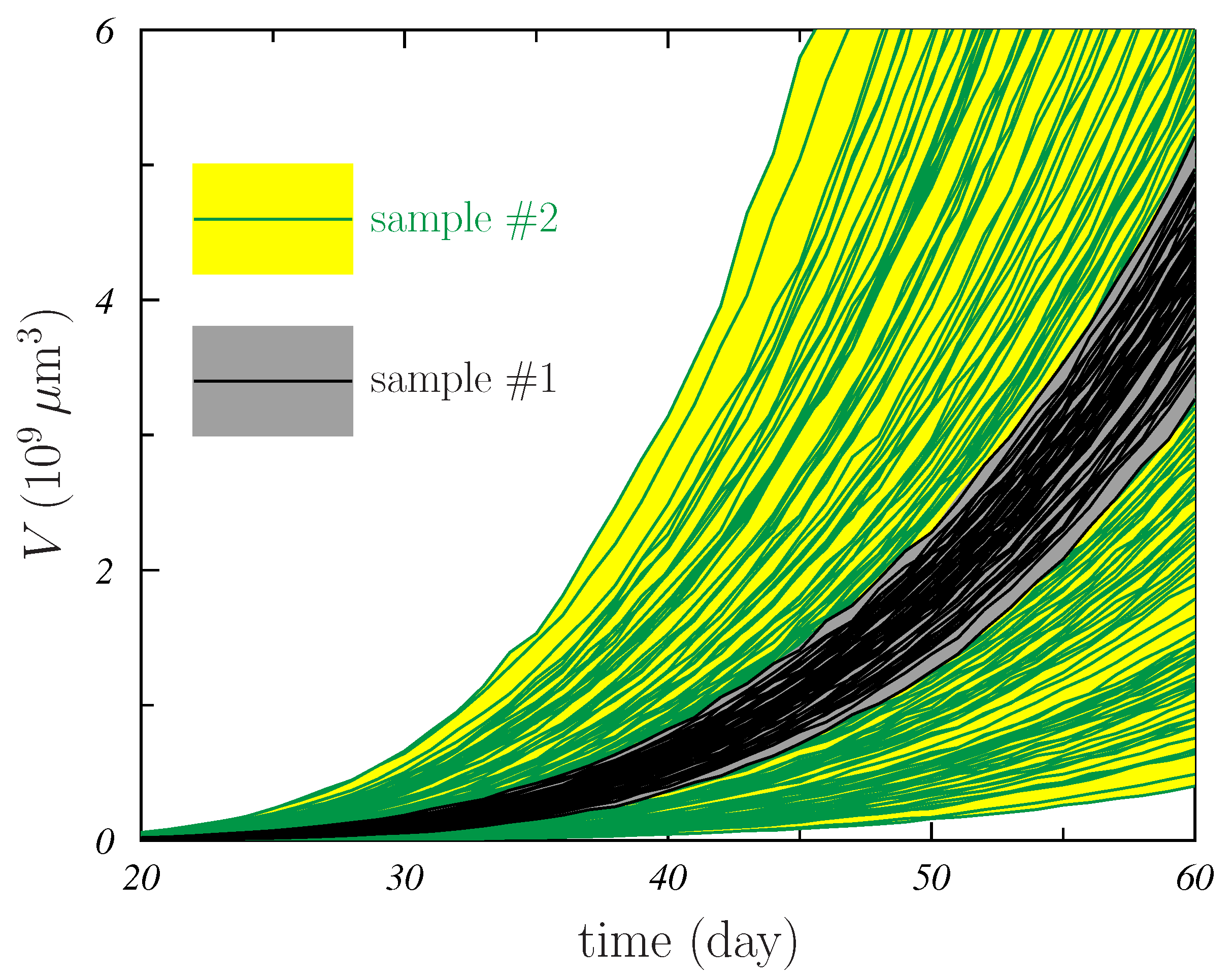
  • For all models, the distributions corresponding to sample #2 were wider than those of sample #1. This is seen in Figure 4 and also in Table 1. The sizes of the 95% CI quoted in the table for sample #2 are larger than those of sample #1 by factors between ∼2 for the G-model and ∼5 for the P-model. In addition, the χ ¯ all found for sample #2 is larger than the corresponding for sample #1, the increase ranging between 0.2 % and 17 % for the G- and B-models, respectively.
    The variability in the AMB parameters that was considered in the simulation generating sample #2 produces more different growth shapes of the MTS and this results in better (those with smaller χ all 2 values) and worst (those with larger χ all 2 ) fits occuring independently of the specific mathematical model considered.
  • In general, the best fits to the whole growth curves were provided by the G-model. As shown in Table 1, the χ ¯ all obtained for this model are an order of magnitude smaller than those corresponding to the other models considered. In the case of sample#1, the 95% CI obtained for the G-model is clearly below those found for the other models. For sample #2, there is a slight overlap between the CI of the G- and P-models.
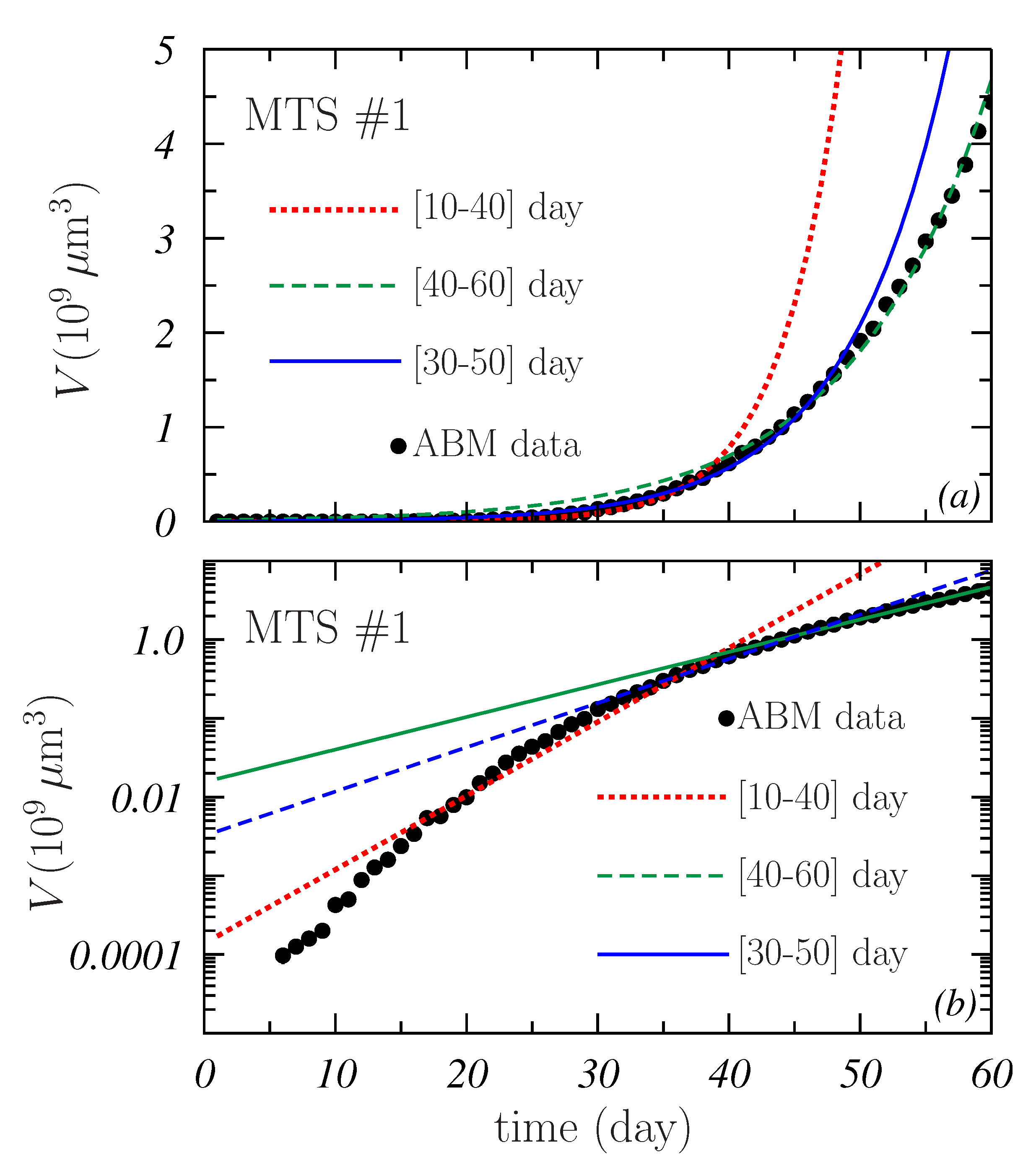
  • It is noticeable the large χ all values obtained for the L-model. The χ ¯ all values are above 170 in both samples, and the respective 95% CI begin at 139 and 56, respectively. This again points out the fact already discussed in connection to Figure 2 about the difficulties of this model to describe the whole MTS growth.
  • A curiosity of these results is that all the distributions are skewed to the right (to high χ all ) except that found for the P-model in the case of sample #1 where an almost Gaussian behavior is observed.
The predictive capabilities of the models were analyzed by looking at how well the models, fitted to reproduce a part of the growth curves, described the remaining volume data. The χ distributions obtained are shown in Figure 5 and Figure 6 and summarized in Table 1 in terms of the corresponding values of χ ¯ and of the 95% CI. In the two figures, the distributions shown in the left panels are those found in the fits, while those calculated for the predicted data are plotted in the right panels. Again, the distributions shown with light colors correspond to sample #2 while those with dark colors were obtained for sample #1.
The results obtained deserve several comments:
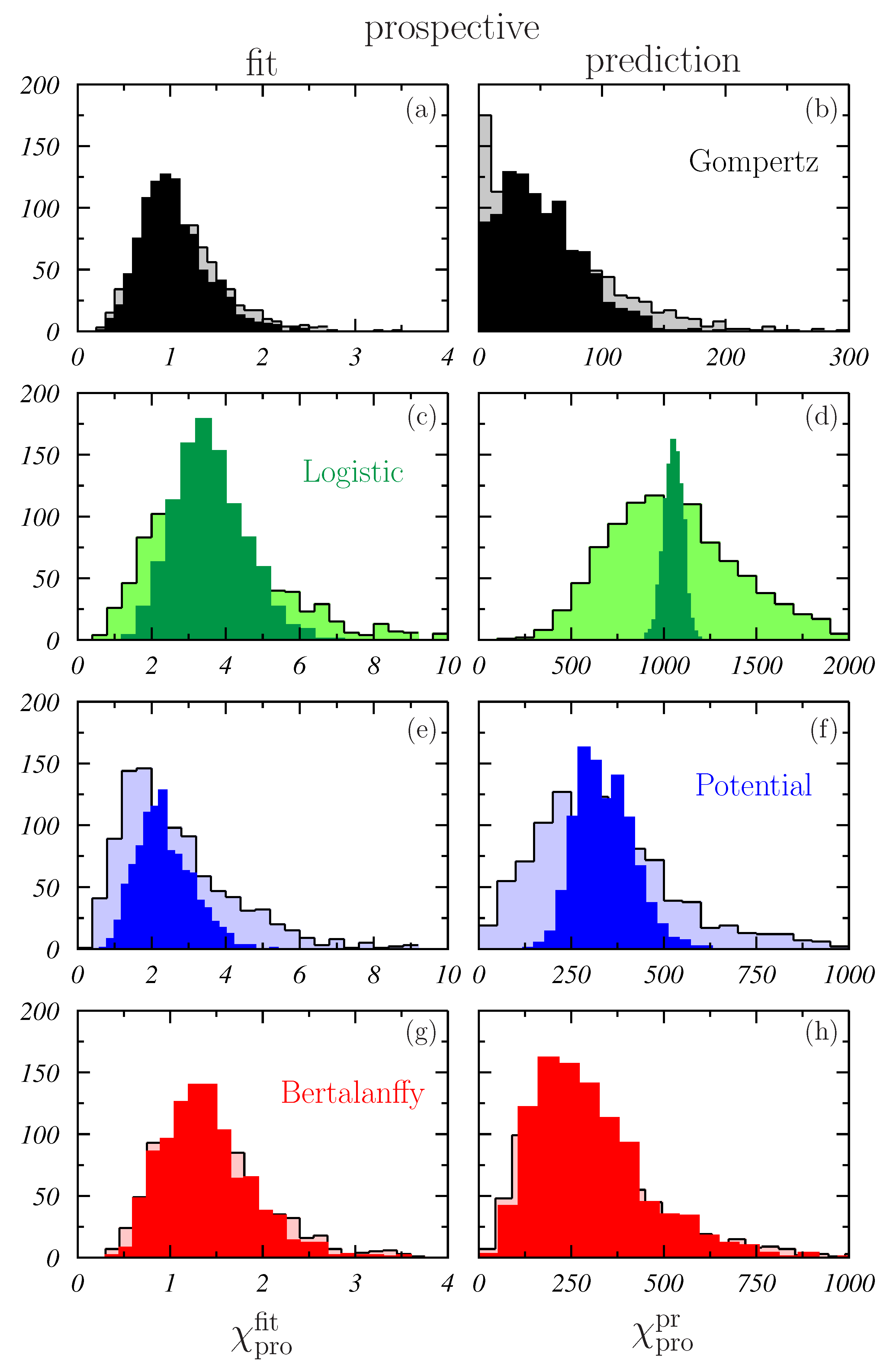
  • The best fits were now much better than those found when all volume data were included. The maximum χ ¯ fit was χ ¯ pro fit = 3.75 , which corresponds to the L-model. These relatively low values are due to the fact that the number of data fitted is now 21 instead of the 55 considered before.
    It is worth noting that also the low limits of the 95% CI of χ fit were much lower than in the case of χ all . In all cases, the values obtained are close to 1, with the only exception of the 1.97 found for the L-model in the prospective prediction (see Table 1). This means that, a priori, all the mathematical models could produce a nice description of a more or less short data section of a given spheroid. However, as pointed out in Figure 4, not all the models can describe the whole growth curve of some of the simulated MTSs included in the samples. In this respect, it is important to point out that, in practice, these mathematical models are fitted to a small number of experimental volume data and for few spheroids or tumors in the sample, and the model that better fits the existing data may not be the one that best describes the subsequent growth [34].
  • Contrary to what was observed in Figure 4, the χ distributions obtained for sample #2 are rather similar to those obtained for sample #1. This is corroborated by the results quoted in Table 1 and may indicate that the main ingredient controlling the results of the fit is the number of points to be fitted.
    An exception to this seems to occur for L- and P-models in the case of the prospective fits (see Figure 6c,e). The possible effect due the region of data fitted is discussed below.
  • As can be checked by comparing the right panels in Figure 5 and Figure 6, the models are more efficient in the retrospective predictions than in the prospective predictions. As it can be seen, the distributions obtained in the latter case extend to values that are at least twice as large as those resulting for the former. The worst situation is that of the B-model in which the ratio χ ¯ pro pr / χ ¯ ret pr 13 . This ratio is ∼2 for G- and L-models and ∼5 for the P-model.
    The retrospective predictive power of the models studied may be of interest in the clinic when the response of tumors to treatments is analyzed. In fact, the evolution of the regression of the irradiated tumors could be similar to looking back at the tumor growth and what has been observed in the present analysis could provide significant hints in that respect. Obviously, treatments may perturb the growth trends and more specific conclusions could be drawn when irradiation is included in the ABM simulation algorithm. Work in this direction is in progress.
  • The best results in what refer to retrospective predictions were provided by the B-model for which the average χ ¯ ret pr 23 (see Table 1). A slightly larger value, ∼30, was found for the G-model, whereas, for the other two models, much higher values are achieved, in particular for the L-model where χ ¯ ret pr 480 .
  • The G-model seems to be the most robust in what refers to the prospective predictive capability. In this case, χ ¯ pro pr < 60 (slightly larger for sample #2 than for sample #1). For P- and B-models, this average was ∼300, while, for the L-model, values larger than 1000 were found.
  • In any case, the values obtained for both χ pro pr and χ ret pr indicate that the predictive capabilities of the models considered here are discrete.
To finish the analysis of the performance of the various mathematical models with regard to the description of the simulated MTS, the goodness of the fits when they are done in different regions of the growth curves was studied. Figure 7 shows the average values of χ reg and the corresponding 95% CI obtained for the four mathematical models as a function of the initial day of the data region fitted (which include 20 consecutive data). Solid circles and uncertainty bars correspond to sample #1, whereas solid curves and light colored areas stand for sample #2.
The following points must be noted:
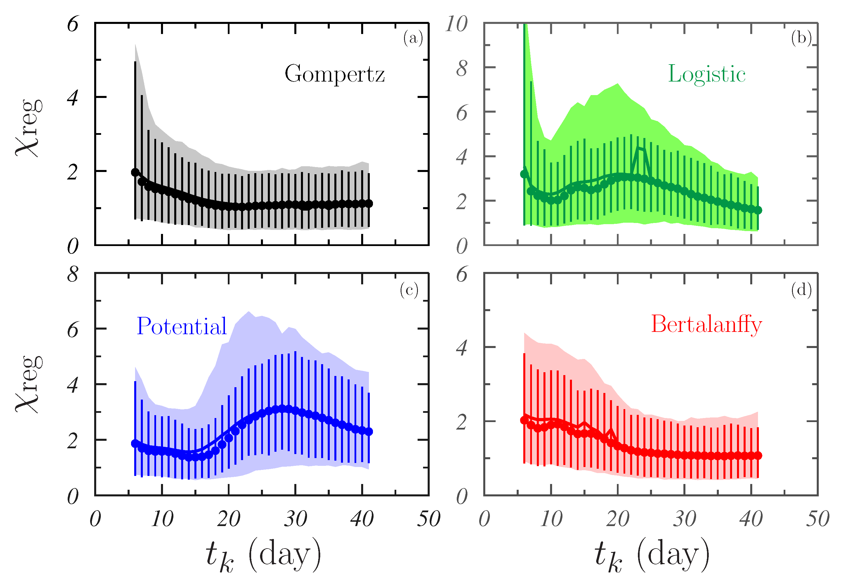
  • Similar results were found for G- and B-models that showed average values tending to 1 with increasing t k . The former appeared to be slightly robust in this sense, showing a less noising behavior for t k < 20 day.
  • For L- and P-models, a non-negligible dependence on the data region fitted occurred. It is worth pointing out the fluctuating behavior with t k observed in both cases.
  • This also results in the differences between the two samples studied being larger for L- and P-models than for G- and B-models.
The analysis that has been done may help to understand how tumors, particularly small tumors that could remain as surgical residues or micro-metastases, evolve before or during radiotherapy, or to investigate the effects provoked by the delays and interruptions that often occur throughout the treatment. In the case of delays in starting radiotherapy, the prospective predictive power of the models is of great interest. For interruptions, both the capacity for retrospection, if the trend of the growth is preserved, and prospection are relevant. These problems can be analyzed with the ABM model and, afterwards, it would be possible to see if the classical models are able to describe what happens in these cases.
The E-model deserves a particular comment. As it has been shown, this model can reproduce the growth curves only when the data considered for the fit are limited to a short time period. On the other hand, its predictive capabilities are very poor. However, in the clinical applications of tumor radiobiology in radiotherapy, only the exponential growth model is used in practice. A relevant example of this is the management of interruptions and delays occurring in fractionated radiotherapy, an important clinical problem due to its effect on the treatment effectiveness [33]. In this case, the exponential growth model is used to account for the increase in tumor cells when the total treatment time is extended and to estimate the effects of this prolongation. As the sole sophistication, the so-called onset time is included. This time attempts to describe, somewhat crudely, the apparent period of slow growth of the tumors that is followed by an increase in the proliferation rate [63] and that occurs as a consequence of the reduction in the tumor cells produced by radiation after a few weeks from the beginning of the treatment [64].
It is evident that MTSs are much simpler systems than in vivo tumors. However, although MTSs are able to reproduce the early stages of the growth of the actual tumors, they do not include several of the elements that most influence the growth of the latter. The results of this work show that the E-model, even for such a simple “approach”, is clearly inefficient for predicting tumor proliferation, and that, on the contrary, other models, such as the G-model, constitute a much more adequate scenario. The G-model also includes, in a simple way, the variation of the growth rate with the tumor size and, therefore, can account for the phenomenon of accelerated repopulation. Our results indicate clearly that it should be necessary to abandon the E-model in favor of any other, maybe the G-model, in clinical applications in order to produce more realistic estimations of the quantities calculated.

4. Conclusions

In this work, a detailed analysis of the capabilities of the Gompertz, logistic, potential, and Bertalanffy models to describe MTS growth curves was carried out. Spheroids simulated with an ABM recently developed were used as “pseudo-experimental” data. Two samples of MTS in which the ABM parameters were assumed to have a different variability were considered.
The best description of the whole growth data was provided by the Gompertz model that showed a value of χ ¯ all an order of magnitude smaller than the other models.
In what refers to the predictive power, Gompertz and Bertalanffy models provided the best retrospective predictions, and the Gompertz model was the one giving the best prospective predictions.
Logistic and potential models had difficulties in fitting the data, even when restricted subsets were considered.
In principle, it is possible to find a certain (reduced) number of spheroids such that one of the models can be fitted to correctly describe a specific part of their growth curves. However, this fitted model does not describe adequately either the remaining volume data of the spheroids included in the fit or the data corresponding to other spheroids in the sample. Usually, experiments of MTS or tumor growth involve quite a few individuals that are followed during a relatively short period and this may explain the “success” of some mathematical models in describing the corresponding growth curves.
In summary, Gompertz model appeared to be the best option to describe the MTS growth data and showed to have enough flexibility to adapt its predictions to the volume growth data variability observed in the simulated spheroids. This indicates that this model should be considered in the clinical applications instead of the exponential model that is currently used.

Author Contributions

Conceptualization, S.R.-A.; D.G.; M.V., and A.M.L.; methodology, S.R.-A., D.G., M.V., and A.M.L.; software, S.R.-A. and A.M.L.; validation, S.R.-A., D.G., M.V., and A.M.L.; formal analysis, S.R.-A., D.G., M.V., and A.M.L.; investigation, S.R.-A., D.G., M.V., and A.M.L.; resources, S.R.-A., D.G., M.V., and A.M.L.; data curation, S.R.-A., D.G., M.V., and A.M.L.; writing—original draft preparation, S.R.-A., D.G., M.V., and A.M.L.; writing—review and editing, S.R.-A.; D.G.; M.V., and A.M.L.; visualization, S.R.-A., D.G., M.V., and A.M.L.; supervision, D.G., M.V., and A.M.L.; project administration, D.G. and M.V.; funding acquisition, S.R.-A., D.G., M.V., and A.M.L. All authors have read and agreed to the published version of the manuscript.

Funding

This work has been partially supported by the Spanish Ministerio de Ciencia y Competitividad (FPA2015-67694-P, PID2019-104888GB-I00), the European Regional Development Fund (ERDF), and the Junta de Andalucía (FQM0387, P18-RT-3237).

Institutional Review Board Statement

Not applicable.

Informed Consent Statement

Not applicable.

Data Availability Statement

The data of the spheroids simulated with the on-lattice agent-based Monte Carlo model are available upon request from the authors.

Conflicts of Interest

The authors declare no conflict of interest.

Abbreviations

The following abbreviations are used in this manuscript:
ABMagent-based model
MTSmulticellular tumor spheroid

References

  1. Sutherland, R.M.; Sordat, B.; Bamat, J.; Gabbert, H.; Bourrat, B.; Mueller-Klieser, W. Oxygenation and differentiation in multicellular spheroids of human colon carcinoma. Cancer Res. 1986, 46, 5320–5329. [Google Scholar] [PubMed]
  2. Cui, X.; Hartanto, Y.; Zhang, H. Advances in multicellular spheroids formation. J. R. Soc. Interface 2017, 14, 20160877. [Google Scholar] [CrossRef]
  3. Oktem, G.; Vatansever, S.; Ayla, S.; Uysal, A.; Aktas, S.; Karabulut, B.; Bilir, A. Effect of apoptosis and response of extracellular matrix proteins after chemotherapy application on human breast cancer cell spheroids. Oncol. Rep. 2006, 15, 335–340. [Google Scholar] [CrossRef] [PubMed]
  4. Pampaloni, F.; Reynaud, E.G.; Stelzer, E.H. The third dimension bridges the gap between cell culture and live tissue. Nat. Rev. Mol. Cell Biol. 2007, 8, 839–845. [Google Scholar] [CrossRef] [PubMed]
  5. Friedrich, J.; Seidel, C.; Ebner, R.; Kunz-Schughart, L.A. Spheroid-based drug screen: Considerations and practical approach. Nat. Protoc. 2009, 4, 309–324. [Google Scholar] [CrossRef]
  6. Labarbera, D.V.; Reid, B.G.; Yoo, B.H. The multicellular tumor spheroid model for high-throughput cancer drug discovery. Expert Opin. Drug Dis. 2012, 7, 819–830. [Google Scholar] [CrossRef]
  7. Pacheco-Marín, R.; Melendez-Zajgla, J.; Castillo-Rojas, G.; Mandujano-Tinoco, E.; Garcia-Venzor, A.; Uribe-Carvajal, S.; Cabrera-Orefice, A.; Gonzalez-Torres, C.; Gaytan-Cervantes, J.; Mitre-Aguilar, I.B.; et al. Transcriptome profile of the early stages of breast cancer tumoral spheroids. Sci. Rep. 2016, 6, 23373. [Google Scholar] [CrossRef] [Green Version]
  8. Mueller-Klieser, W. Three-dimensional cell cultures: From molecular mechanisms to clinical applications. Am. J. Physiol.-Cell Physiol. 1997, 273, C1109–C1123. [Google Scholar] [CrossRef]
  9. Bates, R.C.; Edwards, N.S.; Yates, J.D. Spheroids and cell survival. Crit. Rev. Oncol. Hematol. 2000, 36, 61–74. [Google Scholar] [CrossRef]
  10. Mueller-Klieser, W. Tumor biology and experimental therapeutics. Crit. Rev. Oncol. Hematol. 2000, 36, 123–139. [Google Scholar] [CrossRef]
  11. Kunz-Schughart, L.A.; Freyer, J.P.; Hofstaedter, F.; Ebner, R. The use of 3D cultures for high-throughput screening: The multicellular spheroid model. J. Biomol. Screen. 2004, 9, 273–285. [Google Scholar] [CrossRef] [Green Version]
  12. Conger, A.D.; Ziskin, M.C. Growth of mammalian multicellular tumor spheroids. Cancer Res. 1983, 43, 556–560. [Google Scholar]
  13. Freyer, J.P.; Sutherland, R.M. Selective dissociation and characterization of cells from different regions of multicell tumor spheroids. Cancer Res. 1980, 40, 3956–3965. [Google Scholar]
  14. Guirado, D.; Aranda, M.; Vilches, M.; Villalobos, M.; Lallena, A.M. Dose dependence of the growth rate of multicellular tumour spheroids after irradiation. Br. J. Radiol. 2003, 76, 109–116. [Google Scholar] [CrossRef]
  15. Guirado, D. Variabilidad en Radiobiología. Ph.D. Thesis, University of Granada, Granada, Spain, 2012. [Google Scholar]
  16. Wang, C.; Tang, Z.; Zhao, Y.; Yao, R.; Li, L.; Sun, W. Three-dimensional in vitro cancer models: A short review. Biofabrication 2014, 6, 022001. [Google Scholar] [CrossRef]
  17. McMillan, K.S.; McCluskey, A.G.; Sorensen, A.; Boyd, M.; Zagnoni, M. Emulsion technologies for multicellular tumour spheroid radiation assays. Analyst 2016, 141, 100–110. [Google Scholar] [CrossRef] [PubMed] [Green Version]
  18. Song, Y.; Kim, J.S.; Kim, S.H.; Park, Y.K.; Yu, E.; Kim, K.H.; Seo, E.J.; Oh, H.B.; Lee, H.C.; Kim, K.M.; et al. Patient-derived multicellular tumor spheroids towards optimized treatment for patients with hepatocellular carcinoma. J. Exp. Clin. Cancer Res. 2018, 37, 109. [Google Scholar] [CrossRef]
  19. Sosa, V.I.; Theys, J.; Groot, A.J.; Barbeau, L.M.O.; Lemmens, A.; Yaromina, A.; Losen, M.; Houben, R.; Dubois, L.; Vooijs, M. Synergistic effects of NOTCH/γ-secretase inhibition and standard of care treatment modalities in non-small cell lung cancer cells. Front. Oncol. 2018, 8, 460. [Google Scholar] [CrossRef]
  20. Verjans, E.-T.; Doijen, J.; Luyten, W.; Landuyt, B.; Schoofs, L. Three-dimensional cell culture models for anticancer drug screening: Worth the effort? J. Cell. Physiol. 2018, 233, 2993–3003. [Google Scholar] [CrossRef]
  21. Guirado, D.; Aranda, M.; Ortiz, M.; Mesa, J.A.; Zamora, L.I.; Amaya, E.; Villalobos, M.; Lallena, A.M. Low-dose radiation hyper-radiosensitivity in multicellular tumour spheroids. Br. J. Radiol. 2012, 85, 1398–1406. [Google Scholar] [CrossRef] [Green Version]
  22. Aranda, M. Los Esferoides Multicelulares como test Predictivo de Radiosensibilidad y Radiocurabilidad Tumoral. Ph.D. Thesis, University of Granada, Granada, Spain, 2003. [Google Scholar]
  23. Maruŝić, M.; Bajzer, Z.; Freyer, J.P.; Vuk-Pavlović, S. Analysis of growth of multicellular tumour spheroids by mathematical models. Cell Prolif. 1994, 27, 73–94. [Google Scholar] [CrossRef] [PubMed]
  24. Benzekry, S.; Lamont, C.; Beheshti, A.; Tracz, A.; Ebos, J.M.L.; Hlatky, L.; Hahnfeldt, P. Classical mathematical models for description and prediction of experimental tumor growth. PLoS Comput. Biol. 2014, 10, e1003800. [Google Scholar] [CrossRef] [Green Version]
  25. Vaidya, V.G.; Alexandro, F.J. Evaluation of some mathematical models for tumor growth. Int. J. Biomed. Comput. 1982, 13, 19–36. [Google Scholar] [CrossRef]
  26. Olea, N.; Villalobos, M.; Nuñez, J.; Elvira, J.; Ruiz de Almodóvar, J.M.; Pedraza, V. Evaluation of the growth rate of MCF-7 breast cancer multicellular spheroids using three mathematical models. Cell Prolif. 1993, 27, 213–223. [Google Scholar] [CrossRef]
  27. Wallace, D.I.; Guo, X. Properties of tumor spheroid growth exhibited by simple mathematical models. Front. Oncol. 2013, 3, 51. [Google Scholar] [CrossRef] [Green Version]
  28. Barbolosi, D.; Freyer, G.; Ciccolini, J.; Iliadis, A. Optimisation de la posologie et des modalités d,administration des agents cytotoxiques à l,aide d,un modèle mathématique. Bull. Cancer 2003, 90, 167–175. [Google Scholar] [PubMed]
  29. Swierniak, A.; Kimmel, M.; Smieja, J. Mathematical modeling as a tool for planning anticancer therapy. Eur. J. Pharmacol. 2009, 625, 108–121. [Google Scholar] [CrossRef] [Green Version]
  30. Simeoni, M.; De Nicolao, G.; Magni, P.; Rocchetti, M.; Poggesi, I. Modeling of human tumor xenografts and dose rationale in oncology. Drug Discov. Today Technol. 2013, 10, e365–e372. [Google Scholar] [CrossRef]
  31. Simeoni, M.; Magni, P.; Cammia, C.; De Nicolao, G.; Croci, V.; Presenti, E.; Germani, M.; Poggesi, I.; Rocchetti, M. Predictive pharmacokinetic-pharmacodynamic modeling of tumor growth kinetics in xenograft models after administration of anticancer agents. Cancer Res. 2004, 64, 1094–1101. [Google Scholar] [CrossRef] [PubMed] [Green Version]
  32. Ribba, B.; Watkin, E.; Tod, M.; Girard, P.; Grenier, E.; You, B.; Guiraudo, E.; Freyer, G. A model of vascular tumour growth in mice combining longitudinal tumour size data with histological biomarkers. Eur. J. Cancer 2011, 47, 479–490. [Google Scholar] [CrossRef]
  33. The Royal College of Radiologists. Timely Delivery of Radical Radiotherapy: Guidelines for the Management of Unscheduled Treatment Interruptions, 4th ed.; Ref. No. BFCO(19)1; The Royal College of Radiologists: London, UK, 2019. [Google Scholar]
  34. Murphy, H.; Jaafari, H.; Dobrovolny, H.M. Differences in predictions of ODE models of tumor growth: A cautionary example. BMC Cancer 2016, 16, 163. [Google Scholar] [CrossRef] [Green Version]
  35. Bilous, M.; Serdjebi, C.; Boyer, A.; Tomasini, P.; Pouypoudat, C.; Barbolosi, D.; Barlesi, F.; Chomy, F.; Benzekry, S. Quantitative mathematical modeling of clinical brain metastasis dynamics in non-small cell lung cancer. Sci. Rep. 2019, 9, 13018. [Google Scholar] [CrossRef] [Green Version]
  36. Wei, H.C. Mathematical modeling of tumor growth: The MCF-7 breast cancer cell line. Math. Biosci. Eng. 2019, 16, 6512–6535. [Google Scholar] [CrossRef]
  37. Vaghi, C.; Rodallec, A.; Fanciullino, R.; Ciccolini, J.; Mochel, J.P.; Mastri, M.; Poignard, C.; Ebos, J.L.M.; Benzekry, S. Population modeling of tumor growth curves and the reduced Gompertz model improve prediction of the age of experimental tumors. PLoS Comput. Biol. 2020, 16, e1007178. [Google Scholar] [CrossRef] [Green Version]
  38. Nicolò, C.; Périer, C.; Prague, M.; Bellera, C.; MacGrogan, G.; Saut, O.; Benzekry, S. Machine learning and mechanistic modeling for prediction of metastatic relapse in early-stage breast cancer. JCO Clin. Cancer Inform. 2020, 4, 259–274. [Google Scholar] [CrossRef]
  39. Rockne, R.C.; Hawkins-Daarud, A.; Swanson, K.R.; Sluka, J.P.; Glazier, J.A.; Macklin, P.; Hormuth, D.A., II; Jarrett, A.M.; Lima, E.A.; Oden, J.T.; et al. The 2019 mathematical oncology roadmap. Phys. Biol. 2019, 16, 041005. [Google Scholar] [CrossRef]
  40. Hadjicharalambous, M.; Wijeratne, P.A.; Vavourakis, V. From tumour perfusion to drug delivery and clinical translation of in silico cancer models. Methods 2021, 185, 82–93. [Google Scholar] [CrossRef] [PubMed]
  41. Vera, J.; Lischer, C.; Nenov, M.; Nikolov, S.; Lai, X.; Eberhardt, M. Mathematical modelling in biomedicine: A primer for the curious and the skeptic. Int. J. Mol. Sci. 2021, 22, 547. [Google Scholar] [CrossRef] [PubMed]
  42. Düchting, W.; Lehrig, R.; Rademacher, G.; Ulmer, W. Computer simulation of clinical irradiation schemes applied to in vitro tumor spheroids. Strahlenther. Onkol. 1989, 165, 873–878. [Google Scholar]
  43. Düchting, W.; Ulmer, W.; Ginsberg, T. Cancer: A challenge for control theory and computer modelling. Eur. J. Cancer 1996, 32A, 1283–1292. [Google Scholar] [CrossRef]
  44. Al-Dweri, F.M.O.; Guirado, D.; Lallena, A.M. Simulación de programas fraccionados de radioterapia. Estudio del control tumoral y del efecto de la interrupción del tratamiento. Rev. Fís. Méd. 2001, 2, 17–20. [Google Scholar]
  45. Al-Dweri, F.M.O.; Guirado, D.; Lallena, A.M.; Pedraza, V. Effect on tumour control of time interval between surgery and postoperative radiotherapy: An empirical approach using Monte Carlo Simulation. Phys. Med. Biol. 2004, 49, 2827–2839. [Google Scholar] [CrossRef]
  46. Powathil, G.; Kohandel, M.; Sivaloganathan, S.; Oza, A.; Milosevic, M. Mathematical modeling of brain tumors: Effects of radiotherapy and chemotherapy. Phys. Med. Biol. 2007, 52, 3291–3306. [Google Scholar] [CrossRef] [PubMed]
  47. Powathil, G.G.; Gordon, K.E.; Hill, L.A.; Chaplain, M.A.J. Modelling the effects of cell-cycle heterogeneity on the response of a solid tumour to chemotherapy: Biological insights from a hybrid multiscale cellular automaton model. J. Theor. Biol. 2012, 308, 1–19. [Google Scholar] [CrossRef]
  48. Powathil, G.G.; Adamson, D.J.A.; Chaplain, M.A.J. Towards predicting the response of a solid tumour to chemotherapy and radiotherapy treatments: Clinical insights from a computational model. PLoS Comput. Biol. 2013, 9, e1003120. [Google Scholar] [CrossRef] [PubMed] [Green Version]
  49. Nikolov, S.; Dimitrov, A.; Vera, J. Hierarchical levels of biological systems and their integration as a principal cause for tumour occurrence. Nonlinear Dyn. Psychol. Life Sci. 2019, 23, 315–329. [Google Scholar]
  50. Hamis, S.; Powathil, G.G.; Chaplain, M.A.J. Blackboard to bedside: A mathematical modeling bottom-up approach toward personalized cancer treatments. JCO Clin. Cancer Inform. 2019, 3, 1–11. [Google Scholar] [CrossRef] [Green Version]
  51. Materi, W.; Wishart, D.S. Computational systems biology in cancer: Modeling methods and applications. Gene Regul. Syst. Biol. 2007, 1, 91–110. [Google Scholar] [CrossRef] [Green Version]
  52. Wang, Z.; Butner, J.D.; Kerketta, R.; Cristini, V.; Deisboeck, T.S. Simulating cancer growth with multiscale agent-based modeling. Semin. Cancer Biol. 2015, 30, 70–78. [Google Scholar] [CrossRef] [Green Version]
  53. Ruiz-Arrebola, S.; Tornero-López, A.M.; Guirado, D.; Villalobos, M.; Lallena, A.M. An on-lattice agent-based Monte Carlo model simulating the growth kinetics of multicellular tumor spheroids. Phys. Med. 2020, 77, 194–203. [Google Scholar] [CrossRef] [PubMed]
  54. Yorke, E.D.; Fuks, Z.; Norton, L.; Whitmore, W.; Ling, C.C. Modeling the development of metastases from primary and locally recurrent tumors: Comparison with a clinical data base for prostatic cancer. Cancer Res. 1993, 53, 2987–2993. [Google Scholar]
  55. Spratt, J.A.; Von Fournier, D.; Spratt, J.S.; Weber, E.E. Decelerating growth and human breast cancer. Cancer 1993, 71, 2013–2019. [Google Scholar] [CrossRef]
  56. Von Bertalanffy, L. Quantitative laws in metabolism and growth. Q. Rev. Biol. 1957, 32, 217–231. [Google Scholar] [CrossRef]
  57. West, G.B.; Brown, J.H.; Enquist, B.J. A general model for ontogenetic growth. Nature 2001, 413, 628–631. [Google Scholar] [CrossRef]
  58. Guiot, C.; Degiorgis, P.G.; Delsanto, P.P.; Gabriele, P.; Deisboeck, T.S. Does tumor growth follow a ‘universal law’? J. Theor. Biol. 2003, 225, 147–151. [Google Scholar] [CrossRef] [Green Version]
  59. Herman, A.B.; Savage, V.M.; West, G.B. A quantitative theory of solid tumor growth, metabolic rate and vascularization. PLoS ONE 2011, 6, e22973. [Google Scholar] [CrossRef]
  60. Villalobos, M. Modelos Tumorales en Oncología: Los Esferoides Multicelulares en el Estudio del Cáncer Hormonodependiente. Ph.D. Thesis, University of Granada, Granada, Spain, 1996. [Google Scholar]
  61. Gong, X.; Lin, C.; Cheng, J.; Su, J.; Zhao, H.; Liu, T.; Wen, X.; Zhao, P. Generation of multicellular tumor spheroids with microwell-based agarose xcaffolds for drug testing. PLoS ONE 2015, 10, e0130348. [Google Scholar] [CrossRef] [PubMed] [Green Version]
  62. Press, W.H.; Teukolsky, S.A.; Vetterling, W.T.; Flannery, B.P. Numerical Recipes in FORTRAN. The Art of Scientific Computing; Cambridge University Press: New York, NY, USA, 1995. [Google Scholar]
  63. Withers, H.R.; Taylor, J.M.; Maciejewski, B. The hazard of accelerated tumor clonogen repopulation during radiotherapy. Acta Oncol. 1988, 27, 131–146. [Google Scholar] [CrossRef]
  64. Fowler, J.F. 21 years of biologically effective dose. Br. J. Radiol. 2010, 83, 554–568. [Google Scholar] [CrossRef]
Figure 1. Volume vs. time of growth (in days) corresponding to the two samples generated with the Monte Carlo ABM. The whole regions covered by samples #1 and #2 are indicated in gray and yellow, respectively. Solid lines show some of the simulated MTS growth curves.
Applsci 11 05241 g001
Figure 2. Best fits of the potential (dashed blue lines), Bertalanffy (dotted-dashed red lines), logistic (solid green lines), and Gompertz ( dotted black lines) models to three simulated MTS belonging to sample #1. Black solid circles show the volumes obtained in the ABM simulation. The MTS #138 (a) is the spheroid, among all in sample #1, whose data best fit the potential and Bertalanffy models; the MTS #179 (b) is the spheroid whose data best describe the logistic model, and the MTS #248 (c) is the spheroid whose data best fit the Gompertz model. The values of χ all obtained in each case are also shown.
Applsci 11 05241 g002
Figure 3. In (a), the fits of the exponential model to the simulated ABM data of the MTS #1 of sample #1 are shown. Solid black circles indicate the volumes of this spheroid along the whole time period studied. Dotted red, dashed green, and solid blue lines display the results obtained when the fit involves the data in the time intervals [10–40] day, [40–60] day, and [30–50] day, respectively; (b) shows the corresponding semi-logarithmic plot to emphasize the MTS volume behavior.
Applsci 11 05241 g003
Figure 4. Distribution histograms of the values of χ all obtained in the fits of the four mathematical models considered to all simulated MTS in samples #1 (dark colors) and #2 (light colors). The results obtained for the Gompertz (a), logistic (b), potential (c) and Bertalanffy (d) models are shown.
Applsci 11 05241 g004
Figure 5. Distribution histograms of the values of χ ret obtained in the retrospective fits of the four mathematical models considered to the simulated MTS in samples #1 (dark colors) and #2 (light colors). Left panels correspond to the fits to data in the time interval [40–60] day and right panels to the retrospective fits to data in the time interval [20–39] day. The results obtained for the Gompertz (a,b), logistic (c,d), potential (e,f) and Bertalanffy (g,h) models are shown.
Applsci 11 05241 g005
Figure 6. Distribution histograms of the values of χ pro obtained in the prospective fits of the four mathematical models considered to the simulated MTS in samples #1 (dark colors) and #2 (light colors).Left panels correspond to the fits to data in the time interval [20–40] day and right panels to the prospective fits to data in the time interval [41–60] day. The results obtained for the Gompertz (a,b), logistic (c,d), potential (e,f) and Bertalanffy (g,h) models are shown.
Applsci 11 05241 g006
Figure 7. Values of χ reg obtained in the fits of the four mathematical models considered to the simulated MTS volume data { V i , i = k , k + 19 } with k varying between 6 and 41. Solid circles represent the average values and uncertainty bars indicate that corresponding to the 95% CI calculated for the 1000 spheroids in sample #1. The solid curves and the light color areas indicate the same but for sample #2. The results obtained for the Gompertz (a), logistic (b), potential (c) and Bertalanffy (d) models are shown.
Applsci 11 05241 g007
Table 1. Average values and 95% CI of the χ distributions obtained in the various fits carried out in the present study.
SampleModelAll DataRetrospectiveProspective
χ all χ ret fit χ ret pr χ pro fit χ pro pr
#1G3.231.0929.081.0450.49
[1.89:6.29][0.51:1.82][5.47:68.67][0.49:1.87][3.78:126.70]
L171.491.77478.863.581050.98
[139.06:258.91][0.81:2.95][360.00:613.40][1.97:5.51][956.80:1140.00]
P22.392.5664.592.35340.05
[17.50:27.41][1.34:4.18][44.49:87.20][1.12:3.91][212.30:501.50]
B30.941.0822.991.40304.76
[21.74:46.02][0.50:1.78][4.74:48.63][0.64:2.52][92.49:694.50]
#2G3.791.1129.761.1158.79
[1.29:9.83][0.45:2.19][1.46:94.18][0.44:2.12][1.35:183.90]
L179.481.80480.193.751061.00
[56.72:378.29][0.74:3.55][147.10:959.40][1.14:8.28][467.80:1833.00]
P24.172.6065.142.65340.71
[6.22:57.37][1.12:4.85][15.11:139.60][0.71:6.36][54.31:835.20]
B31.021.0823.371.44315.34
[11.46:64.49][0.46:2.17][4.18:52.42][0.57:2.76][67.76:836.80]
Publisher’s Note: MDPI stays neutral with regard to jurisdictional claims in published maps and institutional affiliations.

