Classification of Apple Disease Based on Non-Linear Deep Features

Abstract

Diseases in apple orchards (rot, scab, and blotch) worldwide cause a substantial loss in the agricultural industry. Traditional hand picking methods are subjective to human efforts. Conventional machine learning methods for apple disease classification depend on hand-crafted features that are not robust and are complex. Advanced artificial methods such as Convolutional Neural Networks (CNN’s) have become a promising way for achieving higher accuracy although they need a high volume of samples. This work investigates different Deep CNN (DCNN) applications to apple disease classification using deep generative images to obtain higher accuracy. In order to achieve this, our work progressively modifies a baseline model by using an end-to-end trained DCNN model that has fewer parameters, better recognition accuracy than existing models (i.e., ResNet, SqeezeNet, and MiniVGGNet). We have performed a comparative study with state-of-the-art CNN as well as conventional methods proposed in the literature, and comparative results confirm the superiority of our proposed model.

1. Introduction

The apple is known as one of the most important tree fruits, due to its second place in world fruit production [1,2]. In the year 2017, the annual production of apples worldwide reached $83.1$ million tons and consumed heavily around the world [1,3]. The high consumption of apples is due to their low cost and numerous healthy properties i.e., high content of fiber, minerals, vitamins, and antioxidants. In addition, its flavor offers the possibility of consuming them naturally or using them for innumerable derived products. It is estimated that approximately $33\%$ of apples produced worldwide are processed to make juices, ciders, applesauce, alcoholic beverages, and dried apples, among other products [4].

In recent years, the production of the apple industry is facing significant loss due to diseases that cause poor quality of the product. Minimal observation through a naked eye can distinguish and identify the diseased apple from the rest. However, human analysis is highly subjective and prone to error. Therefore, an accurate and timely diagnosis of diseases is a fundamental and extremely critical process to avoid future losses. There are many apple diseases according to a phytopathology datasheet [5,6], but the most common diseases are Blotch, Rot, and Scab.

Several studies suggest that visual exploration through hand-picked methods are the most used methods in fruit disease diagnosis. However, it is a slow and problematic process [7,8]. Conventional methods such as Polymerase Chain Reaction (PCR) require detailed molecular sampling, resulting in a non-cost-effective technique [9]. In recent years, Artificial Intelligence (AI) has been used to help experts in the automatic diagnosis of diseases that affect plants and trees. The methods performed with AI are faster, less expensive, and more efficient [10,11,12].

Machine learning (ML) is defined as a branch of AI that automates the construction of analytical models so that systems can learn from large amounts of data, identify patterns, and make decisions [13,14,15]. Nevertheless, in most cases, traditional ML approaches applied to complex images have non-automatic feature extraction steps [16,17], reducing the effectiveness and making the process more time-consuming, and accuracy may not be satisfactory [18,19,20]. Whereas, Deep Learning (DL) is an advanced form of ML modeling that allows systems to train themselves and improve classification accuracy through a series of calculations based on multiple layers of non-linear processing units [21,22,23]. The advantage of DL is the ability to exploit raw data without using hand-crafted features, and without prior knowledge, to extract relevant features [24,25,26,27].

Enormous studies have been carried out to identify and classify apple diseases. For instance, Goel et al. [28] proposed a method to classify healthy apples and three types of diseases (Blotch, Rot, and Scab). The authors hybridized three metaheuristic algorithms to segment apple images using the maximization function between groups for clustering and segmentation. Local Binary Pattern (LBP)-based features are extracted from segmented images for classification using Multiclass Support Vector Machine (MSVM). Li et al. [29] introduced an apple disease classification technique using a back-propagation-based Artificial Neural Network (ANN). The model is trained using healthy and fungal-infected apple images, to which the methods of eliminating the background, segmentation of apple defects, and identification of the calyx and stem are applied to obtain the features for the network. In 2012, Dubey et al. [7] presented a solution to detect Blotch, Rot, and Scab apple diseases using an MSVM classification technique. The apple images are segmented using the K-means clustering technique followed by feature extraction using the Global Color Histogram (GCH), Color Coherence Vector (CVC), LBP, and Complete Local Binary Pattern (CLBP). These features are fed to MSVM to classify among the different apple diseases.

Later in 2016, Dubey et al. [30] used another method to investigate the same set of apple images by using a combined unique feature descriptor instead of separate feature descriptors. First, the images are segmented using the K-means grouping technique to obtain the features of color, texture, and shape of the apples. Then, apple diseases are classified using MSVM with an average accuracy of $95.6\%$. In 2019, Ayyub et al. [31] obtained an accuracy of $96.29\%$ by classifying the same apple images. Ayyub et al. proposed a method that consists of the extraction of features using the Improved Summation and Difference Histogram (ISADH), Complete Local Binary Patterns (CLBP), and Zernike Moments (ZM).

In addition to the works discussed above (i.e., classical/conventional ML), many researchers tend to work on DL such as Convolutional Neural Networks (CNN), a popular technique for image recognition, which has demonstrated outstanding ability in image processing and classification [24,32]. Wang et al. [33] evaluated the performance of transfer learning using pre-trained DL models to classify images of healthy apple leaves and apple leaf black Rot in three stages (i.e., early stage, middle stage, and final stage). According to experimental results, the highest performance obtained is $90.4\%$ with the VGG16 model. Furthermore, Alharbi and Arif [25] collected 800 images for each of the four diseases (i.e., blotch, rot, scab, and healthy). They further augment the dataset using basic operations such as flips, scale, crop, illumination to generate 3200 images for each disease.

Several other similar studies (similar to the ones discussed above) have been conducted by different researchers, for instance, Nachtigall et al. [34] proposed a method to detect and classify the nutritional deficiencies and herbicide damage in apple trees, using leaf images and AlexNet. Liu et al. [35] worked in the identification of four types of apple leaf diseases (i.e., Mosaic, Rust, Brown spot, and Alternaria leaf spot) based on AlexNet. Al-Shawwa and Abu-Naser [36] implemented a method for the classification of 13 different apple species using Deep Convolutional Neural Network (DCNN). Turkoglu et al. [37] applied a hybrid method between Long Short-Term Memory (LSTM) architecture with pre-trained DCNN models. The features are extracted with transfer learning and fed to the LSTM to detect pests and diseases with an average accuracy of $99.2\%$. The higher accuracies are obtained using DL approaches for the classification of apple leaf diseases. One of the most prominent advantages of DCNN is its ability to execute non-linear features [38,39]. DCNN automatically detects the essential features without any human supervision [40,41]. DCNN is computationally efficient since it uses a particular convolution, special pooling operations, and performs parameter sharing. Additionally, DCNN can solve difficult applications such as classification, image segmentation and location inspection [42,43,44,45,46,47,48,49].

To the best of our knowledge, there are very limited existing approaches that directly handle apple disease classification problems similar to the one addressed in this article. Therefore, this paper proposes an approach to classify the apple diseases based on Deep Convolutional Generative Adversarial Network (DCGAN) data and DCNN-based on two different architectures. DCGAN model is used to overcome the limitations of the limited availability and validation of apple disease images. Thus, DCGAN generates new (to some extent, similar to the original) images, which helps to train a DCNN model to obtain higher accuracy in apple disease classification.

The rest of the paper is structured as; Section 2 explains the material and methods used in this study. Section 3 contains information regarding the experimental results and discussion. Finally, Section 4 concludes the paper with possible future research directions.

2. Materials and Methods

This section explains the dataset used in this study and the generation of synthetic images using deep convolutions. Furthermore, this section also discusses the deep learning architecture used for the classification of apple diseases.

2.1. Dataset Description

The original dataset used in this work contains 319 (i.e., 80 images for healthy, Blotch, and Rot Apple images, respectively, and 79 for Scab) images of apples in which some are healthy, and others are from apples with any of the three, Blotch, Rot, and Scab diseases. These images are obtained from a set of the dataset used in works [7,9,30,31], which is publically available at the Kaggle repository. This small dataset is further used to create 4000 synthetic images through the Deep Convolutional Generative Adversarial Network (DCGAN) architecture, from which 1000 images are for each of the four categories are generated to construct an optimal DL solution.

2.2. Deep Convolutional Generative Adversarial Network (DCGAN)

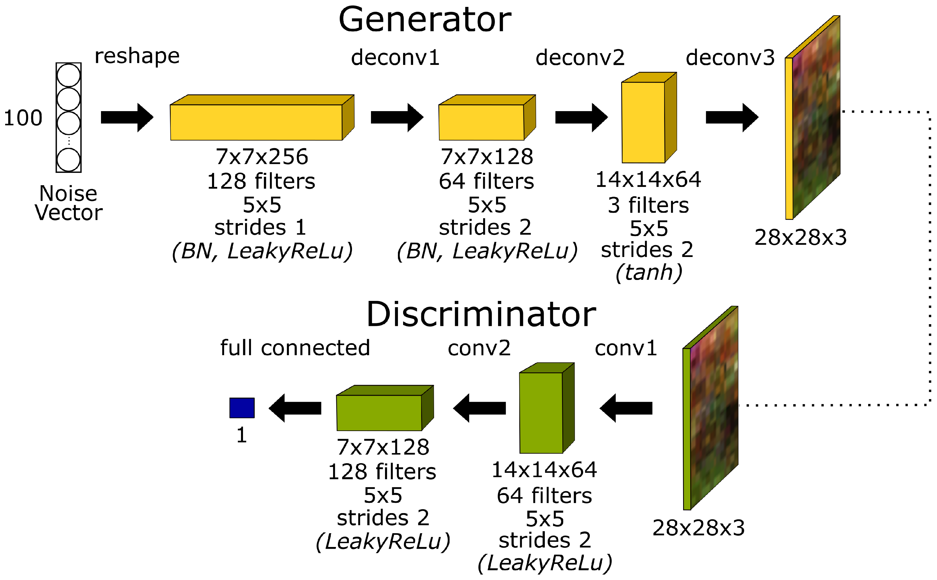
As explained in Section 2.1, DCGAN architecture is used to generate synthetic images to train a DL model. DCGAN implicitly learns from the distribution of data contained in a set of sample images to create new images extracted from the learned distribution. DCGAN is faster than traditional GAN architecture because DCNN is modified instead of ANN to increase stability and convergence [50]. The model used in this study consists of two DCNNs that are trained simultaneously. The first model is the generator, and the second is the discriminator; these models work with only convolutional layers to learn up and down spatial samples independently. The main aim of the generator is to construct fake noise data into an image that fools the discriminator to classify it as a fake image. While the discriminator aims to identify if the image is fake or real, at the end of the training, the generator can produce the image that is indistinguishable from real data, recreating the original data distribution [51].

The discriminator model is a convolutional process that eliminates the fully connected layer and uses the LeakyReLu as an activation function to compress an image into a feature vector. The generator model is a deconvolution process in which all activation functions use LeakyReLu, except the output layer that uses tanh. The overall network works through the Equation (1) [52].

$$V(D,G)=E_{X\sim P_{data}\left(X\right)}\left[logD\left(x\right)\right]+E_{z\sim P_Z\left(Z\right)}\left[log(1-D\left(G\left(Z\right)\right))\right]$$

(1)

where D and G represent generator and discriminator, whereas X represents a sample that is transformed by the generator through noise vector Z. D defines the training target for G to distinguish between real sample $p_{data}\left(X\right)$ and generated one $P_z\left(Z\right)$. Therefore, the generator will confuse the discriminator to predict that the generated data is true or real. Figure 1 shows the DCGAN structure used in this work to increase the size of the dataset. The generative network consists of three deconvolution layers of 128, 64, and 3 filters, respectively, with a $5\times 5$ kernel. The first two layers used the LeakyReLu activation function and the Batch Normalization (BN). The BN is used to normalize the input layer by adjusting and scaling the activation, while the last layer used tanh as an activation function. The discriminative network consists of two convolutional layers of 64 and 128 filters with a $5\times 5$ kernel. The LeakyReLu activation function is used for both layers. Further information regarding the layer-wise settings can be found in

Table 1. The summary of the proposed models.

DCNN			DCGAN-based DCNN
Layers	Size	# of Param	Layers	Size	# of Param
Input Layer	$350\times 350\times 3$	—	Input Layer	$32\times 32\times 3$	—
Conv_1	$348\times 348\times 128$	3584	Conv_1	$30\times 30\times 128$	3584
Maxpooling	$174\times 174\times 128$	—	Conv_2	$28\times 28\times 64$	73,792
Conv_2	$172\times 172\times 64$	73,792	Dropout_1	$28\times 28\times 64$	—
Maxpooling	$86\times 86\times 64$	—	Conv_3	$26\times 26\times 64$	36,928
Conv_3	$86\times 86\times 64$	36,928	Conv_4	$24\times 24\times 32$	18,464
Maxpooling	$42\times 42\times 64$	—	Maxpooling	$12\times 12\times 32$	—
Conv_4	$40\times 40\times 32$	18,464	Dropout_2	$12\times 12\times 32$	—
MaxPooling	$20\times 20\times 32$	—	Conv_5	$10\times 10\times 32$	9248
Conv_5	$18\times 18\times 32$	9248	Maxpooling	$5\times 5\times 32$	—
MaxPooling	$9\times 9\times 32$	—	Dropout_3	$5\times 5\times 32$	—
Flatten	2592	—	Flatten	800	—
Dropout_1	2592	—	Dense_1	256	205,056
Dense_1	256	663,808	Dropout_4	256	—
Dropout_2	256	—	Dense_2	128	32,896
Dense_2	# of Classes	1028	Dense_3	# of Classes	516
Total Parameters = 806,852			Total Parameters = 380,484

.

2.3. Deep Convolutional Neural Network

Nowadays, Deep Convolutional Neural Network (DCNN) has been explored for series of 2D and 3D datasets [26]. AlexNet [53], ResNet, Mini-VGGNet, and SqueezeNet are considered as state-of-the-art DL networks for medical imaging, food processing, and fruit disease detection tasks. Therefore, in this work, AlexNet architecture is used a based model, which uses minimal convolutional operations to the input data using 2D kernels (presented in Equation (2)) to extract the feature maps (i.e., output maps) [54].

$$A_{nm}^{xy}=f\left(\sum _{c=o}^{C_m-1}\sum _{r=0}^{R_m-1}{K}_{nm}^{cr}{A}_{(n-1)}^{(x+c)(y+r)}+b_{nm}\right),$$

(2)

where $A_{nm}^{xy}$ is the output feature at $[x,y]$, n indicates the layers, m represents the number of feature maps, b is the bias, $K_{nm}^{cr}$ gives the value at ($c,r$) of the kernel connected to the $m_{th}$ feature map, with C and R being the entire height and width of the kernel. Finally, $f(.)$ represents the activation function (ReLu in our case) respectively. Normally, the disease region is usually smaller than the rest of the apple percentage, as shown in Figure 2 and Table 1. Given this, we first automatically focused on the feature extraction of the disease region and confined a fully connected feature map at the FC-layer(fully connected) for classification. Further information regarding the layer-wise settings can be found in Table 1.

2.4. Optimizer and Loss Function

In DL, step size also refers to the learning rate is the most concerning issue and causes redundancies. For example, a large step may diverge instead of converging, or a small size may make take longer for a network to converge. Thus, for the aforesaid reasons, several optimization algorithms are considered during the training of the dataset, which includes Adam, AdaGrad, Adamax, and Nadam, among others. In this study, for multi-class classification, categorical cross-entropy is employed as a loss function. The comparison within the class can be predicted through the Equation (3) [55], where P and p represent the expected and the target values of the function N respectively.

$$N(p,P)=-\sum _{a=0}^H\sum _{b=0}^W(p_{ab}\ast log\left(P_{ab}\right))$$

(3)

2.5. Evaluation Metrics

Overall (OA) accuracy is rigorously used for comparative analysis. As in the literature, this work also used the same metric to analyze the generalization performance of our proposed model. The OA can be computed as follows:

$$\mathrm{OA}=\frac{1}{C}\sum _{i=1}^{C}T{P}_i$$

(4)

where $TP$ is a true positive and C is the total number of classes. In addition to the OA, we have also performed a statistical test called the z-test. In this test, the confidence interval is a type of statistical estimation in which the intervals are associated with confidence concerning the true parameters of the proposed model. The confidence interval $\lambda$ is then obtained by the given observations, i.e., a valid probability of containing the true underlying parameters. There are many possibilities to choose a level of confidence, such as a $90\%$ confidence interval that defines the hypothetical indefinite data collection; furthermore, it estimates the population parameter. Therefore, it is required to choose an appropriate confidence level before examining the data. In a nutshell, in this work, a $95\%$ confidence level is used. However, the values of the confidence level of $99\%$ or $90\%$ are also often used for several applications. The confidence interval is then computed as in the following steps.

• Compute sample mean i.e., $\mu =\overline{x}$.
• Identify the standard deviation $\sigma$ is known otherwise compute the standard deviation i.e., $\delta$.
  • If the standard deviation is known then $z^{*}={\mathsf{\Phi }}^{-1}(1-\frac{\alpha }{2})={\mathsf{\Phi }}^{-1}\left(\frac{\alpha }{2}\right)$, where $C=100(1-\alpha )\%$ is confidence level and $\mathsf{\Phi }$ is the cumulative density function of the standard normal distribution used as a critical value.
  • If the standard deviation is unknown then the t distribution is used as a critical value point which depends on the confidence level C for the degrees of freedom (DoF). The DoF can be found by subtracting one of the number of observations i.e., $(n-1)$. The critical values are as follows: $C=99\%$, $z^{*}=2.576$, $C=98\%$, $z^{*}=2.326$, $C=95\%$, $z^{*}=1.96$ and $C=90\%$, $z^{*}=1.645$. Thus, the critical value can be expressed as $t^{*}-t_{\alpha }\left(r\right)$ where r be the degree of freedom and $\alpha =\frac{1-C}{2}$.
• Thus, by plugging the values into the appropriate equations:
  • For a known standard deviation:

    $$\left(\overline{x}-z^{*}\frac{\sigma }{\sqrt{n}},\overline{x}+z^{*}\frac{\sigma }{\sqrt{n}}\right)$$

    (5)
  • For an unknown standard deviation:

    $$\left(\overline{x}-t^{*}\frac{\delta }{\sqrt{n}},\overline{x}+t^{*}\frac{\delta }{\sqrt{n}}\right)$$

    (6)

where $\mu =\overline{x}=\frac{1}{n}{\sum }_{i=1}^N{x}_i$ is sample mean. $\delta =\sqrt{\frac{1}{n-1}{\sum }_{i=1}^N{(x_i-\mu )}^2}$.

3. Results and Discussion

The dataset was divided into 70% for training and 30% for blind testing. The 70% training dataset is further divided into 90/10% for training and validation sets using a 10-fold cross-validation process. Therefore DCGAN-DCNN is originally trained and validated on 3023 images and tested on the remaining 1295 images with a spatial size of $32\times 32\times 3$ per image.

This section further illustrates the experimental evaluation of apple disease classification through several experiments along with a statistical test. All the listed experiments are performed on the online platform Google Colab using the Jupyter environment as back-end [56]. The run-time of the environment is a GPU with a python 3 notebook, with 25 GB of Random Access Memory (RAM) and 358.27 GB of cloud storage for data computation. Initially, the experiments are done on original data (without including the synthetic images) with a size of $350\times 350$ and then further analyzed on the DCGAN-dataset with the size of $32\times 32$. Some examples of the generated images are shown in Figure 3. There are similar features between the generated images and the original images. However, it is important to highlight that the generated images are of comparatively low resolution due to the filter sizes, which is due to the availability of a limited resource. Higher filter sizes may produce more accurate images with higher resolution, however, as earlier explained, it requires to have more powerful computational resources.

The structure of the DCNN model used in this study consists of a sequential model since it has equivalent dimensions for each input and output. A 2D kernel of size $(3\times 3)$ is used that will pass the filters throughout the image for the convolution operation for each convolution layer. To stride down and reduce the noisy features from the segmented images, a max-pooling layer is used with the ReLu. Further information regarding the layer-wise settings can be found in Table 1. After the convolutional operators, the flatten layer is used with 205,056 features and a dropout of $0.25$ to cope with the over-fitting issues. These FC layers features are then dense to give four class labeled classification for apple disease detection with softmax using several optimizers (i.e., Adam, Adamax, Nadam, and Adadelta).

For DL models, the learning rate is sensitive; therefore, in this work, for each optimizer, we set a standard step size as Adam = $0.001$, Adadelta = $1.0$, Nadam = $0.002$, and Adamax = $0.002$ for training. $Bet{a}_1$ and $Bet{a}_2$ parameters are observed to be close to 1 for Adam, Nadam, and Adamax; similarly, the $\rho$ parameter for Adadelta is greater than 0 with no delay parameter. Moreover, for the DCNN model, the loss function is compiled to be “categorical-correspondence” to separate the diseases into four classes. DCGAN model works on the small spatial size of each class, i.e., $32\times 32\times 3$ and thus converge on lesser iterations, i.e., 10 epochs for each optimizer, and requires some tuning in its structure as shown in Figure 4. Whereas, for a larger size, data are compiled and trained on using 35 epochs for the original dataset.

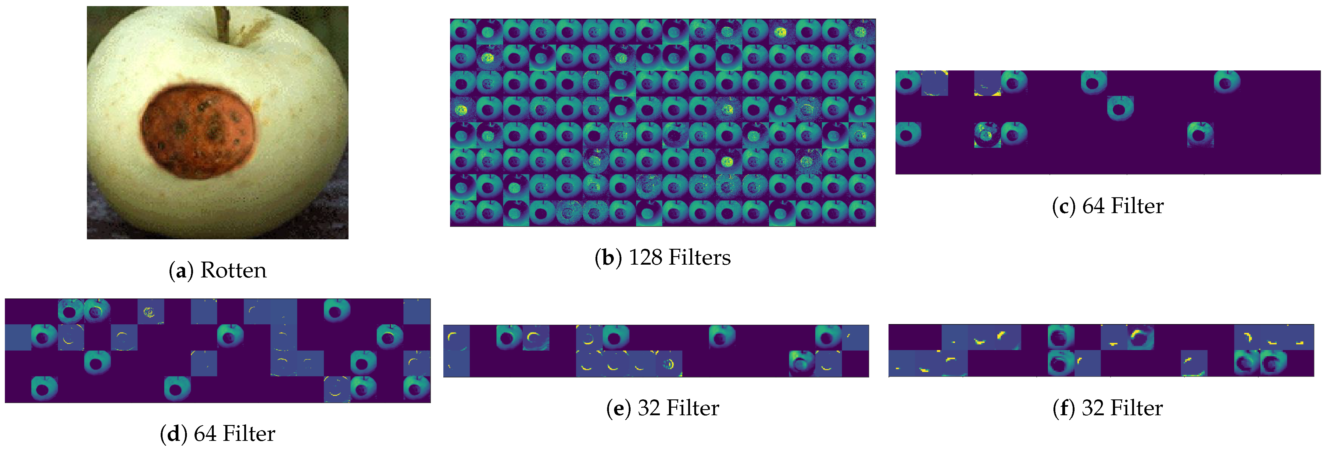
Compared with the conventional methods that mostly rely on hand-crafted features, the DCNN model achieved higher statistical significance and accuracy. This is because the deep models provide non-linear features as shown in Figure 5 that preserve the significant spatial information about the object for Rotten Apple image (Figure 5a) is used as a visual example. Figure 5b–f represents the feature maps learned by applying 128, 64, 64, 32 and 32 filters respectively.

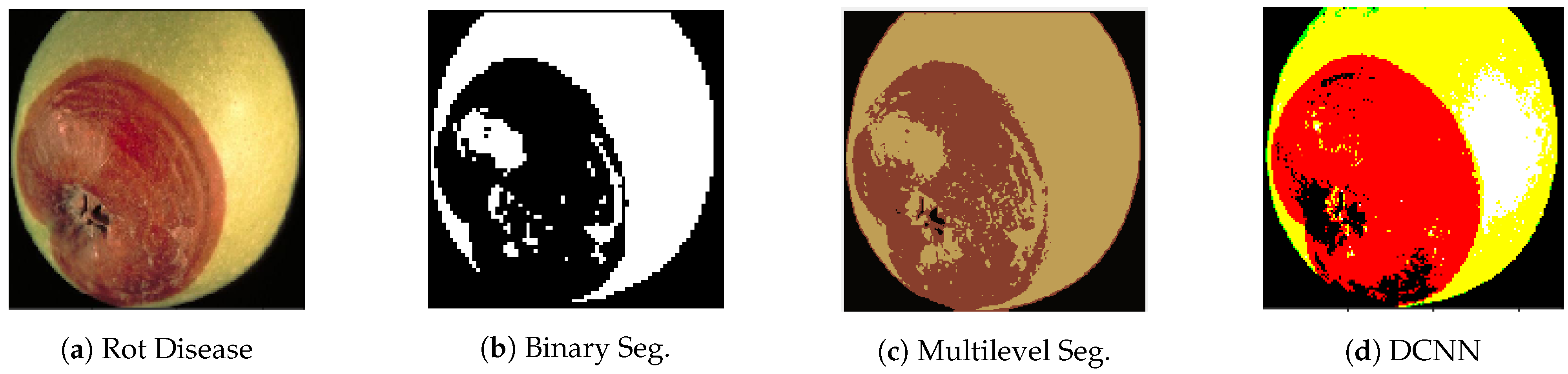
As mentioned above, DL extract features in more depth such as edges, color, corner, and shape rather than conventional segmentation and clustering-based methods. For instance, Figure 6a, Figure 7a and Figure 8a present the input image, whereas Figure 6b, Figure 7b and Figure 8b showed the results obtained using a binary segmentation process. Meanwhile, Figure 6c, Figure 7c and Figure 8c present the output obtained through the multilevel segmentation. For all these experiments, Otsu’s global thresholding method is used for binary segmentation, whereas multilevel segmentation is obtained through three-points K-means clustering for each RGB color sequence. Multilevel segmentation is commonly used to highlight the defects by partitioning the images in different clusters [7,30]. All these results are compared with the DCNN model as shown in Figure 6d, Figure 7d and Figure 8d. From these results, one can conclude that the proposed model obtained significantly higher results as compared to the binary and multilevel segmentation as well as several other hand-crafted feature-based classification.

In previous studies, the accuracy of the apple disease classification is examined along with multiple techniques. These techniques extract features to form a feature descriptor in order to achieve an accuracy rate of $93\%$ to $95.6\%$. Furthermore, the classification techniques have also been analyzed through color, texture, and shape-based features. All of these studies used an MSVM as a baseline classifier to classify different diseases in apples. The comparative study is shown in

Table 2. Experimental evaluation with and without synthetic examples as compared to the state-of-the-art as well as conventional methods. The higher accuracies are in bold face.

Model	Blotch	Scab	Rot	Healthy	OA(%)
State-of-the-art and Conventional Methods
2D CNN	99.00%	99.99%	91.00%	99.99%	99.17%
ResNet50	99.99%	99.00%	76.00%	99.99%	96.00%
MiniVggNet	99.99%	60.90%	20.00%	84.42%	69.00%
SqueezeNet	99.99%	99.99%	91.00%	99.99%	99.00%
ISADH+GLCM+MSVM	99.99%	98.57%	99.90%	95.71%	96.00%
GCH+LBP+MSVM	88.46%	85%	89.72%	86.66%	90.80%
CCV+CLBP+ZM+MSVM	97.50%	93.75%	92.50%	99.90%	95.60%
HSV+CLBP+MSVM	89.88%	90.71%	96.66%	99.33%	93.00%
Proposed Method without synthetic examples
DCNN-Adam	99.99%	99.99%	99.99%	99.99%	99.99%
DCNN-Adamax	93.00%	93.00%	99.99%	99.99%	96.66%
DCNN-Nadam	99.99%	86.66%	86.66%	99.99%	93.00%
DCNN-Adadalta	99.9%	99.99%	73.33%	86.66%	88.00%
Proposed Method with synthetic examples
DCGAN-DCNN-Adam	99.99%	99.99%	99.99%	99.99%	99.99%
DCGAN-DCNN-Adamax	99.00%	99.00%	99.99%	99.99%	99.66%
DCGAN-DCNN-Adadalta	99.99%	99.00%	99.00%	99.99%	99.00%
DCGAN-DCNN-Nadam	99.99%	98.00%	99.99%	99.99%	98.00%

explains the accuracy achieved by DCNN with several optimizers. Adam’s optimizer learning rate converges effectively for this work than other optimizers and produces remarkable results compared to the several conventional hand-crafted features-based classification techniques.

Moreover, the state of art deep learning models such as ResNet (https://www.kaggle.com/yadavsarthak/residual-networks-and-mnist (accessed on 25 February 2021)), SqeezeNet (https://www.kaggle.com/somshubramajumdar/squeezenet-for-mnist (accessed on 26 February 2021)) and MiniVGGNet (https://www.pyimagesearch.com/2019/02/11/fashion-mnist-with-keras-and-deep-learning (accessed on 11 February 2019)) have been analyzed in comparison with the proposed DCGAN-DCNN model. All of these models have several numbers of convolutional operations and require keen observations in setting up a number of kernels and filters. The layer-wise settings for these models, along with the proposed model are presented in

Table 3. Layer-wise settings of all comparative models.

—	ResNet	SqueezeNet	MiniVGGNet	Proposed
Kernels	$32,64,32,64,32,64,32$	$128,128,128,64,64,64,32,32,32$	$128,128,64,64$	$128,64,64,32,32$
Batch size	55	55	55	55
Filters size	$(3\times 3),(3\times 3)$	$(1\times 1),(1\times 1),(3\times 3)$	$(3\times 3)$	$(3\times 3)$
Activation Function	relu	relu	relu	relu
Optimizer	Adam	Adam	Adam	Adam

. All the competing methods are analyzed with different optimizers through a 10-fold cross-validation process. From experimental results, one can conclude that the proposed DCGAN-DCNN model outperformed with an overall accuracy of $99.99\%$ in comparison with other state-of-the-art models. The complete pipeline comparison with the abovementioned methods can be seen in Table 2.

4. Conclusions

This study proposed a DCGAN-DCNN model for apple disease, i.e., Blotch, Rot, and Scab classification. The DCNN structure consists of five convolutional, two dense, and one decision vector layer to classify the apple disease. Experimental results reveal that the proposed model outperformed several conventional and state-of-the-art deep models. However, the learning rate and optimizer have a strong influence; therefore, an appropriate selection of these two essential hyper-parameters is critical to get better results. Future research entails incorporating the soft and hard attentional mechanism in deep models for apple disease classification.

References

- Musacchi, S.; Serra, S. Apple fruit quality: Overview on pre-harvest factors. Sci. Hortic. 2018, 234, 409–430. [Google Scholar] [CrossRef]
- Cebulj, A.; Cunja, V.; Mikulic-Petkovsek, M.; Veberic, R. Importance of metabolite distribution in apple fruit. Sci. Hortic. 2017, 214, 214–220. [Google Scholar] [CrossRef]
- Faostat, F. Food and agriculture organization of the United Nations (FAO) 2017. Available online: http://www.fao.org/faostat/en/-data/QC (accessed on 2 April 2021).
- Skinner, R.C.; Gigliotti, J.C.; Ku, K.M.; Tou, J.C. A comprehensive analysis of the composition, health benefits, and safety of apple pomace. Nutr. Rev. 2018, 76, 893–909. [Google Scholar] [CrossRef]
- Hartman, J. Apple Fruit Diseases Appearing at Harvest; Plant Pathology Fact Sheet, College of Agriculture, University of Kentucky: Lexington, KY, USA, 2010. [Google Scholar]
- Sindhi, K.; Pandya, J.; Vegad, S. Quality evaluation of apple fruit: A Survey. Int. J. Comput. Appl. 2016, 975, 8887. [Google Scholar] [CrossRef]
- Ram Dubey, S.; Singh Jalal, A. Adapted Approach for Fruit Disease Identification using Images. Int. J. Comput. Vis. Image Process. 2012, 20, 317–330. [Google Scholar] [CrossRef]
- Barbedo, J.G.A. Digital image processing techniques for detecting, quantifying and classifying plant diseases. SpringerPlus 2013, 2, 660. [Google Scholar] [CrossRef] [Green Version]
- Dubey, S.R.; Jalal, A.S. Fusing color and texture cues to identify the fruit diseases using images. Int. J. Comput. Vis. Image Process. 2014, 4, 52–67. [Google Scholar] [CrossRef]
- Qin, F.; Liu, D.; Sun, B.; Ruan, L.; Ma, Z.; Wang, H. Identification of alfalfa leaf diseases using image recognition technology. PLoS ONE 2016, 11, e0168274. [Google Scholar] [CrossRef] [Green Version]
- Rajan, P.; Radhakrishnan, B.; Suresh, L.P. Detection and classification of pests from crop images using support vector machine. In Proceedings of the 2016 International Conference on Emerging Technological trends (ICETT), Kollam, India, 21–22 October 2016; pp. 1–6. [Google Scholar]
- Islam, M.; Dinh, A.; Wahid, K.; Bhowmik, P. Detection of potato diseases using image segmentation and multiclass support vector machine. In Proceedings of the 2017 IEEE 30th Canadian Conference on Electrical and Computer Engineering (CCECE), Windsor, ON, Canada, 30 April–3 May 2017; pp. 1–4. [Google Scholar]
- Ahmad, M.; Shabbir, S.; Oliva, D.; Mazzara, M.; Distefano, S. Spatial-prior Generalized Fuzziness Extreme Learning Machine Autoencoder-based Active Learning for Hyperspectral Image Classification. Opt. Int. J. Light Electron Opt. 2020, 206, 163712. [Google Scholar] [CrossRef]
- Maheshwari, D.; Garcia-Zapirain, B.; Sierra-Soso, D. Machine learning applied to diabetes dataset using Quantum versus Classical computation. In Proceedings of the 2020 IEEE International Symposium on Signal Processing and Information Technology (ISSPIT), Louisville, KY, USA, 9–11 December 2020. [Google Scholar]
- Ahmad, M.; Khan, A.; Khan, A.M.; Mazzara, M.; Distefano, S.; Sohaib, A.; Nibouche, O. Spatial Prior Fuzziness Pool-Based Interactive Classification of Hyperspectral Images. Remote Sens. 2019, 11, 1136. [Google Scholar] [CrossRef] [Green Version]
- Ahmad, M.; Khan, A.M.; Hussain, R. Graph-based spatial spectral feature learning for hyperspectral image classification. IET Image Process. 2017, 11, 1310–1316. [Google Scholar] [CrossRef]
- Ahmad, M.; Alqarni, M.A.; Khan, A.M.; Hussain, R.; Mazzara, M.; Distefano, S. Segmented and Non-Segmented Stacked Denoising Autoencoder for Hyperspectral Band Reduction. Opt. Int. J. Light Electron Opt. 2018, 180, 370–378. [Google Scholar] [CrossRef] [Green Version]
- Jiang, P.; Chen, Y.; Liu, B.; He, D.; Liang, C. Real-time detection of apple leaf diseases using deep learning approach based on improved convolutional neural networks. IEEE Access 2019, 7, 59069–59080. [Google Scholar] [CrossRef]
- Ahmad, M.; Khan, A.M.; Mazzara, M.; Distefano, S. Multi-layer Extreme Learning Machine-based Autoencoder for Hyperspectral Image Classification. In Proceedings of the 14th International Conference on Computer Vision Theory and Applications (VISAPP’19), Prague, Czech Republic, 25–27 February 2019. [Google Scholar] [CrossRef]
- Liu, J.; Yang, S.; Cheng, Y.; Song, Z. Plant leaf classification based on deep learning. In Proceedings of the 2018 Chinese Automation Congress (CAC), Xi’an, China, 30 November–2 December 2018; pp. 3165–3169. [Google Scholar]
- Isik, S.; Özkan, K. Overview of handcrafted features and deep learning models for leaf recognition. J. Eng. Res. 2021, 9. [Google Scholar] [CrossRef]
- Maeda-Gutierrez, V.; Galvan-Tejada, C.E.; Zanella-Calzada, L.A.; Celaya-Padilla, J.M.; Galván-Tejada, J.I.; Gamboa-Rosales, H.; Luna-Garcia, H.; Magallanes-Quintanar, R.; Guerrero Mendez, C.A.; Olvera-Olvera, C.A. Comparison of convolutional neural network architectures for classification of tomato plant diseases. Appl. Sci. 2020, 10, 1245. [Google Scholar] [CrossRef] [Green Version]
- Hameed, Z.; Zahia, S.; Garcia-Zapirain, B.; Javier Aguirre, J.; María Vanegas, A. Breast cancer histopathology image classification using an ensemble of deep learning models. Sensors 2020, 20, 4373. [Google Scholar] [CrossRef] [PubMed]
- Li, L.; Zhang, S.; Wang, B. Plant Disease Detection and Classification by Deep Learning—A Review. IEEE Access 2021, 9, 56683–56698. [Google Scholar] [CrossRef]
- Alharbi, A.G.; Arif, M. Detection and Classification of Apple Diseases Using Convolutional Neural Networks. In Proceedings of the 2020 2nd International Conference on Computer and Information Sciences (ICCIS), Sakaka, Saudi Arabia, 13–15 October 2020; pp. 1–6. [Google Scholar]
- Ahmad, M.; Khan, A.M.; Mazzara, M.; Distefano, S.; Ali, M.; Sarfraz, M.S. A Fast and Compact 3-D CNN for Hyperspectral Image Classification. IEEE Geosci. Remote Sens. Lett. 2020, 1–5. [Google Scholar] [CrossRef]
- Nanni, L.; Ghidoni, S.; Brahnam, S. Handcrafted vs. non-handcrafted features for computer vision classification. Pattern Recognit. 2017, 71, 158–172. [Google Scholar] [CrossRef]
- Goel, L.; Raman, S.; Dora, S.S.; Bhutani, A.; Aditya, A.; Mehta, A. Hybrid computational intelligence algorithms and their applications to detect food quality. Artif. Intell. Rev. 2019, 53, 1415–1440. [Google Scholar] [CrossRef]
- Li, Q.; Wang, M.; Gu, W. Computer vision based system for apple surface defect detection. Comput. Electron. Agric. 2002, 36, 215–223. [Google Scholar] [CrossRef]
- Dubey, S.R.; Jalal, A.S. Apple disease classification using color, texture and shape features from images. Signal Image Video Process. 2016, 10, 819–826. [Google Scholar] [CrossRef]
- Ayyub, S.R.N.M.; Manjramkar, A. Fruit Disease Classification and Identification using Image Processing. In Proceedings of the 2019 3rd International Conference on Computing Methodologies and Communication (ICCMC), Erode, India, 27–29 March 2019; pp. 754–758. [Google Scholar]
- Kamilaris, A.; Prenafeta-Boldú, F.X. Deep learning in agriculture: A survey. Comput. Electron. Agric. 2018, 147, 70–90. [Google Scholar] [CrossRef] [Green Version]
- Wang, G.; Sun, Y.; Wang, J. Automatic image-based plant disease severity estimation using deep learning. Comput. Intell. Neurosci. 2017, 2017, 2917536. [Google Scholar] [CrossRef] [Green Version]
- Nachtigall, L.G.; Araujo, R.M.; Nachtigall, G.R. Classification of apple tree disorders using convolutional neural networks. In Proceedings of the 2016 IEEE 28th International Conference on Tools with Artificial Intelligence (ICTAI), San Jose, CA, USA, 6–8 November 2016; pp. 472–476. [Google Scholar]
- Liu, B.; Zhang, Y.; He, D.; Li, Y. Identification of apple leaf diseases based on deep convolutional neural networks. Symmetry 2018, 10, 11. [Google Scholar] [CrossRef] [Green Version]
- Al-Shawwa, M.O.; Abu-Naser, S.S. Classification of Apple Fruits by Deep Learning. Int. J. Acad. Eng. Res. 2019, 3, 1–7. [Google Scholar]
- Turkoglu, M.; Hanbay, D.; Sengur, A. Multi-model LSTM-based convolutional neural networks for detection of apple diseases and pests. J. Ambient. Intell. Humaniz. Comput. 2019. [Google Scholar] [CrossRef]
- Minaee, S.; Abdolrashidi, A. Deep-emotion: Facial expression recognition using attentional convolutional network. arXiv 2019, arXiv:1902.01019. [Google Scholar]
- Sharif Razavian, A.; Azizpour, H.; Sullivan, J.; Carlsson, S. CNN features off-the-shelf: An astounding baseline for recognition. In Proceedings of the IEEE Conference on Computer Vision and Pattern Recognition Workshops, Columbus, OH, USA, 24–27 June 2014; pp. 806–813. [Google Scholar]
- Minaee, S.; Boykov, Y.; Porikli, F.; Plaza, A.; Kehtarnavaz, N.; Terzopoulos, D. Image Segmentation Using Deep Learning: A Survey. arXiv 2020, arXiv:2001.05566. [Google Scholar]
- Ahmad, M.; Mazzara, M.; Distefano, S. Regularized CNN Feature Hierarchy for Hyperspectral Image Classification. Remote Sens. 2021, 13, 2275. [Google Scholar] [CrossRef]
- Saber, A.; Sakr, M.; Abo-Seida, O.M.; Keshk, A.; Chen, H. A Novel Deep-Learning Model for Automatic Detection and Classification of Breast Cancer Using the Transfer-Learning Technique. IEEE Access 2021, 9, 71194–71209. [Google Scholar] [CrossRef]
- Acosta, M.F.J.; Tovar, L.Y.C.; Garcia-Zapirain, M.B.; Percybrooks, W.S. Melanoma diagnosis using deep learning techniques on dermatoscopic images. BMC Med. Imaging 2021, 21, 6. [Google Scholar]
- Fan, H.; Du, W.; Dahou, A.; Ewees, A.A.; Yousri, D.; Elaziz, M.A.; Elsheikh, A.H.; Abualigah, L.; Al-Qaness, M.A. Social Media Toxicity Classification Using Deep Learning: Real-World Application UK Brexit. Electronics 2021, 10, 1332. [Google Scholar] [CrossRef]
- Bogaerts, T.; Masegosa, A.D.; Angarita-Zapata, J.S.; Onieva, E.; Hellinckx, P. A graph CNN-LSTM neural network for short and long-term traffic forecasting based on trajectory data. Transp. Res. Part C Emerg. Technol. 2020, 112, 62–77. [Google Scholar] [CrossRef]
- Arteaga, B.; Diaz, M.; Jojoa, M. Deep Learning Applied to Forest Fire Detection. In Proceedings of the 2020 IEEE International Symposium on Signal Processing and Information Technology (ISSPIT), Louisville, KY, USA, 9–11 December 2020; pp. 1–6. [Google Scholar]
- Sahlol, A.T.; Yousri, D.; Ewees, A.A.; Al-Qaness, M.A.; Damasevicius, R.; Abd Elaziz, M. COVID-19 image classification using deep features and fractional-order marine predators algorithm. Sci. Rep. 2020, 10, 15364. [Google Scholar] [CrossRef] [PubMed]
- Canizo, M.; Triguero, I.; Conde, A.; Onieva, E. Multi-head CNN–RNN for multi-time series anomaly detection: An industrial case study. Neurocomputing 2019, 363, 246–260. [Google Scholar] [CrossRef]
- AL-Alimi, D.; Shao, Y.; Feng, R.; Al-Qaness, M.A.; Elaziz, M.A.; Kim, S. Multi-scale geospatial object detection based on shallow-deep feature extraction. Remote Sens. 2019, 11, 2525. [Google Scholar] [CrossRef] [Green Version]
- Goodfellow, I.; Pouget-Abadie, J.; Mirza, M.; Xu, B.; Warde-Farley, D.; Ozair, S.; Courville, A.; Bengio, Y. Generative adversarial nets. In Advances in Neural Information Processing Systems; MIT Press: Cambridge, MA, USA, 2014; pp. 2672–2680. [Google Scholar]
- Radford, A.; Metz, L.; Chintala, S. Unsupervised representation learning with deep convolutional generative adversarial networks. arXiv 2015, arXiv:1511.06434. [Google Scholar]
- Fang, W.; Zhang, F.; Sheng, V.S.; Ding, Y. A method for improving CNN-based image recognition using DCGAN. CMC Comput. Mater. Contin. 2018, 57, 167–178. [Google Scholar] [CrossRef]
- Hinton, G.E.; Srivastava, N.; Krizhevsky, A.; Sutskever, I.; Salakhutdinov, R.R. Improving neural networks by preventing co-adaptation of feature detectors. arXiv 2012, arXiv:1207.0580. [Google Scholar]
- Li, Y.; Zhang, H.; Shen, Q. Spectral–spatial classification of hyperspectral imagery with 3D convolutional neural network. Remote Sens. 2017, 9, 67. [Google Scholar] [CrossRef] [Green Version]
- Mzoughi, H.; Njeh, I.; Wali, A.; Slima, M.B.; BenHamida, A.; Mhiri, C.; Mahfoudhe, K.B. Deep multi-scale 3D convolutional neural network (CNN) for MRI gliomas brain tumor classification. J. Digit. Imaging 2020, 33, 903–915. [Google Scholar] [CrossRef] [PubMed]
- Carneiro, T.; Da Nóbrega, R.V.M.; Nepomuceno, T.; Bian, G.B.; De Albuquerque, V.H.C.; Reboucas Filho, P.P. Performance Analysis of Google Colaboratory as a Tool for Accelerating Deep Learning Applications. IEEE Access 2018, 6, 61677–61685. [Google Scholar] [CrossRef]