Structural Design and Optimization of Herringbone Grooved Journal Bearings Considering Turbulent

Abstract

In order to improve the performance of the traditional constant-width herringbone grooved journal bearing in a computed tomography tube under a high-temperature environment, the present study designed a convergent herringbone grooved journal bearing (HGJB) structure lubricated by liquid metal. The bearing oil film thickness and the Reynolds equation considering the influence of turbulence are established and solved by using the finite difference method in the oblique coordinate system. The performance of the two bearings was compared, and the static and dynamic performance change trends of the two bearing structures under different eccentricities were systematically studied. The results show that the convergent herringbone grooved journal bearings are superior to the constant-width herringbone grooved journal bearings in terms of bearing capacity and stiffness coefficient. At the same time, the influence of structural parameters, such as the number of grooves, helix angle, groove to ridge ratio, groove depth on the performance of the constant-width herringbone grooved journal bearings, and the convergent herringbone grooved journal bearings was studied. Finally, we conclude that the performance of the convergent herringbone grooved journal bearings is optimal when the number of grooves is 15–20, the helix angle is 30°–45°, the ratio of the groove to ridge is 1, and the groove depth is 0.02 mm –0.024 mm. This research has provided the thinking and reference basis for the design of liquid metal bearings for high-performance CT equipment.

1. Introduction

Computed tomography is a combination of the rapid development of computer technology and X-ray technology in modern times [1]. The CT machine using this technology is an indispensable device for modern clinical diagnosis, and it plays an increasingly important role in the medical field. The CT ball tube is the core component of the CT equipment, and it is expensive. On the one hand, the performance of the CT ball tube must meet the requirements of high speed, high definition of CT imaging, high power, and high reliability. On the other hand, it is hoped that it has a longer life and lower cost [2]. The continuous popularization of CT machines has brought a huge market demand for CT ball tubes, so the development of CT ball tubes with superior performance is of great significance and market value.

The anode target located in the CT tube spirally moves around the patient to obtain a three-dimensional image of the patient. In recent years, in order to shorten the diagnosis time and improve the image resolution, the anode target speed has become higher and higher, and the centrifugal force on the CT tube has also greatly increased, which has made the previous rolling bearings that used solid lubricants to load no longer applicable [3]. Compared with rolling bearings, journal bearings run more smoothly and can better meet the requirements of supporting anode targets. The CT tube is small in size and requires high sealing performance, so an external oil supply system cannot be used. Because the structure of the herringbone groove bearing is relatively compact, it can realize self-lubrication, self-sealing, good stability, low temperature rise, long working life, and other characteristics; and become a good choice for CT ball tube bearings [4,5,6]. When the rotation speed of the bearing increases, the temperature of the lubricating medium will increase significantly, and the viscosity will decrease, and the bearing capacity will decrease, which is prone to accidents [7,8]. Due to the high-temperature and high-vacuum working environment in the CT tube, the bearing lubricating medium supporting the high-speed rotation of the anode target needs to meet the requirements of high temperature resistance, high thermal conductivity and low vapor pressure. Due to a large amount of research on liquid metals in recent years, it is possible to find a lubricant that satisfies such conditions. Among them, the performance of gallium-based liquid metals is the most prominent. Gallium-based liquid metal has relatively low viscosity, high thermal conductivity, certain inertness, nontoxicity, and good stability [9]. At the same time, the vapor pressure of gallium metal is particularly low compared to other liquid metals, and it still remains liquid in a high vacuum state, so it can be used in a high vacuum environment. Many of the latest CT equipment use gallium-based liquid metal for lubrication, such as the IMRC tube produced by Philips, which abandons the traditional ball or roller bearing structure and adopts a new spiral groove bearing. The unique liquid metal lubricant has greatly improved the heat dissipation rate.

The research on herringbone grooved journal bearings mainly focuses on the optimization of the performance of the herringbone grooves and their structural parameters [10,11,12]. Eliott et al. used herringbone grooves to improve bearing performance [13,14,15]. Hirs [16] analyzed the bearing performance of three distribution forms of herringbone grooves. The results show that herringbone grooved journal bearings have good and predictable stability characteristics and can run stably at the center and near-center positions. At the same time, experiments were carried out to verify the correctness of the theoretical results. Kang et al. [17] conducted a related study on the performance characteristics of herringbone grooved journal bearings with an arc-shaped bottom surface based on the finite difference method and found that the oil film load capacity is worse than that of a smooth journal bearing. Gad et al. [18] proposed a bearing with a stepped bottom surface. By optimizing geometric parameters, a larger oil film bearing load capacity and stiffness were obtained. Afterwards, Murata et al. [19] first studied and analyzed herringbone grooved journal bearings on a two-dimensional plane and found that the surface morphology of the herringbone groove can improve the stability of the bearing. Bonneau et al. [20] found that when the eccentricity is smaller, the stiffness coefficient of the herringbone grooved journal bearing is greater than that of the ordinary smooth journal bearing, and its bearing load capacity is effectively improved, which attributed to the pumping effect and step effect of the herringbone grooved journal bearing. Li et al. [21] analyzed the static and dynamic performance of herringbone grooved journal bearings under turbulent flow and slip conditions. Yang et al. [22] studied the influence of herringbone groove structure parameters on the performance of thrust bearings and obtained bearing structure parameters that make the bearing perform well. Han et al. [23,24] used a new elastic fluid lubrication numerical algorithm to analyze the influence of different chevron bottom shapes on bearing performance. As a result, the triangle on the left side of the surface can significantly improve bearing lubrication performance.

Liquid metal is an amorphous and flowable metal. The amorphous liquid form of liquid metal gives it excellent electrical and thermodynamic properties. It is currently widely used in batteries, power equipment, biomedical, 3D printing, and computing fields [25,26,27]. In the 1960s, it was found that the application of liquid metal to the nuclear power magnetohydrodynamic bearing can greatly improve the bearing load capacity [28]. Persad et al. [29] of the University of Texas studied the common liquid metal phenomenon at the armature–rail interface. They found that the solid armature track will not corrode when lubricated by the quenched metal deposit of the liquid aluminum. Liu Weimin [30,31,32,33] of Northwestern Polytechnical University made a preliminary evaluation of the antifriction performance of gallium-based liquid metal. In their friction experiments, they found that the surface of the material lubricated with gallium liquid metal had no obvious dent, while the surface of the material not lubricated with gallium liquid metal had obvious wear. Li Yi and others of the State Key Laboratory of Solid Lubrication, Lanzhou Institute of Chemical Physics, Chinese Academy of Sciences [34] used the SRV-IV friction and wear tester to carry out the lubrication performance experiment of liquid metal in a wide temperature range from −10 °C to 800 °C. The results show that the liquid metal exhibits excellent tribological properties at −10 °C and 20 °C. Jing et al. [35] of Beijing Aerospace Long March Aircraft Research Institute studied the flow of liquid metal in U-shaped pipes under the influence of magnetohydrodynamics. The results of the numerical simulation show that when the flow enters the central area of the U-shaped flow channel, a spiral flow is formed. Its stirring effect may be beneficial to the heat exchange in the pipeline.

At present, only a few people are conducting research on the performance of bearings lubricated with liquid metal. Due to the low viscosity of liquid metal, this paper adopts a turbulent flow calculation model and considers the special structure of the herringbone grooves. At present, the groove width of the herringbone grooved journal bearing studied is constant. In order to improve the performance of the traditional constant-width herringbone grooved journal bearings, the convergent herringbone grooved journal bearings were designed. At the same time, the influence of the eccentricity, groove number, helix angle, and other structural parameters of the herringbone grooved journal bearing on bearing performance was studied, and the best structural parameters of the bearing were determined.

2. Numerical Model and Digital Simulation

Herringbone groove journal bearings are a circle of herringbone grooves machined on the smooth surface of the sliding bearing. The groove width of the traditional herringbone grooved journal bearing is equal everywhere, but the groove of the herringbone grooved journal bearing designed in this paper is convergent. That is to say, the groove width is not a fixed value. In the following introduction, the constant-width HGJBs refer to the traditional constant-width herringbone grooved journal bearings, and the convergent HGJBs refer to the newly designed convergent herringbone grooved journal bearings. The schematic diagram of the bearing structure is shown in Figure 1. Figure 1a shows the front view of the bearings, Figure 1b shows the constant-width HGJBs, and Figure 1c shows the convergent HGJBs.

2.1. Establishment of Reynolds Equation

2.1.1. Static Reynolds Equation

For the HSJBs, the influence of turbulence must be considered because of the liquid metal lubricants used, which has a low viscosity. The expression of the static Reynolds equation of an incompressible fluid at a constant temperature in a Cartesian coordinate system is [36]:

$$\frac{\partial }{\partial x}\left(\frac{h^3}{\mu }{G}_x\frac{\partial p}{\partial x}\right)+\frac{\partial }{\partial z}\left(\frac{h^3}{\mu }{G}_z\frac{\partial p}{\partial z}\right)=\frac{U}{2}\frac{\partial h}{\partial x}$$

(1)

In the formula: $x$ is the bearing radius. $p$ is the oil film pressure. $\mu$ is lubricant viscosity. $\omega$ is the journal angular velocity. $G_x$ and $G_z$ are the flow regime coefficients. Under laminar flow, $G_x=G_z=1/12$.

Substituting $U=r\omega$, $x=r\phi$ and the turbulence factors $k_x=1/G_x$, $k_z=1/G_z$ into Equation (1), the radial dimensionless Reynolds equation in cylindrical coordinates can be obtained:

$$\frac{\partial }{\partial \phi }\left(\frac{H^3}{k_x}\frac{\partial P}{\partial \phi }\right)+{\left(\frac{d}{b}\right)}^2\frac{\partial }{\partial \lambda }\left(\frac{H^3}{k_z}\frac{\partial P}{\partial \lambda }\right)=\frac{1}{4}\frac{\partial H}{\partial \phi }$$

(2)

In the formula: $k_x=12+0.0136{\left(R_e\right)}^{0.90}$; $k_z=12+0.0043{\left(R_e\right)}^{0.96}$. The dimensionless quantity used is $\phi =\frac{x}{r}$, $\lambda =\frac{z}{b/2}$, $H=\frac{h}{c}$, and $P=\frac{p}{p_0}$. Where $p_0=\frac{2\omega r^2\mu }{c^2}$ is the dimensionless pressure coefficient, and $c$ is the bearing radius clearance.

2.1.2. Dynamic Reynolds Equation

For the HSJBs, in the static equilibrium position, considering the slight movement of the journal, the dynamic Reynolds equation under unsteady conditions is obtained as:

$$\frac{\partial }{\partial x}\left(\frac{h^3}{\mu }{G}_x\frac{\partial p}{\partial x}\right)+\frac{\partial }{\partial z}\left(\frac{h^3}{\mu }{G}_z\frac{\partial p}{\partial z}\right)=\frac{U}{2}\frac{\partial h}{\partial x}+\frac{\partial h}{\partial t}$$

(3)

In the formula: $\frac{\partial h}{\partial t}=\dot{e}\cos \phi +e\dot{\theta }\sin \phi$.

Substituting $\dot{\epsilon }=\frac{\dot{e}}{c\omega }$, $\epsilon {\theta }^{\prime }=\frac{e\dot{\theta }}{c\omega }$, and the dimensionless quantities of the static Reynolds equation into the above formula, the dimensionless dynamic Reynolds equation is obtained:

$$\frac{\partial }{\partial \phi }\left(\frac{H^3}{k_x}\frac{\partial P}{\partial \phi }\right)+{\left(\frac{d}{b}\right)}^2\frac{\partial }{\partial \lambda }\left(\frac{H^3}{k_z}\frac{\partial P}{\partial \lambda }\right)=\frac{1}{4}\frac{\partial H}{\partial \phi }+\frac{1}{2}\frac{\partial H}{\partial \overline{t}}$$

(4)

Taking the derivative of $P$ with respect to $\mathsf{\Delta }\epsilon$, $\epsilon \mathsf{\Delta }\theta$, ${\epsilon }^{\prime }$, and $\epsilon {\theta }^{\prime }$, the equations for the disturbance pressure $P_{\epsilon }$, $P_{\theta }$, $P_{{\epsilon }^{\prime }}$, and $P_{{\theta }^{\prime }}$ will be:

$$\mathrm{Re}y\left(P_{\epsilon }\right)=-\frac{1}{4}\sin \phi -\left(\frac{\partial }{\partial \phi }\left(\frac{3H^2}{k_x}\cos \phi \frac{\partial P}{\partial \phi }\right)+{\left(\frac{d}{b}\right)}^2\frac{\partial }{\partial \lambda }\left(\frac{3H^2}{k_z}\cos \phi \frac{\partial P}{\partial \lambda }\right)\right)$$

(5)

$$\mathrm{Re}y\left(P_{\theta }\right)=-\frac{1}{4}\cos \phi -\left(\frac{\partial }{\partial \phi }\left(\frac{3H^2}{k_x}\sin \phi \frac{\partial P}{\partial \phi }\right)+{\left(\frac{d}{b}\right)}^2\frac{\partial }{\partial \lambda }\left(\frac{3H^2}{k_z}\sin \phi \frac{\partial P}{\partial \lambda }\right)\right)$$

(6)

$$\mathrm{Re}y\left(P_{{\epsilon }^{\prime }}\right)=\frac{1}{2}\cos \phi$$

(7)

$$\mathrm{Re}y\left(P_{{\theta }^{\prime }}\right)=\frac{1}{2}\sin \phi$$

(8)

In the formula: $\mathrm{Re}y(\sim )$ represents $\frac{\partial }{\partial \phi }\left(\frac{H^3}{k_x}\cos \phi \frac{\partial (\sim )}{\partial \phi }\right)+{\left(\frac{d}{b}\right)}^2\frac{\partial }{\partial \lambda }\left(\frac{H^3}{k_z}\cos \phi \frac{\partial (\sim )}{\partial \lambda }\right)$; $P_{\epsilon }=\frac{\partial P}{\partial \epsilon }$; $P_{\theta }=\frac{\partial P}{\epsilon \partial \theta }$; $P_{{\epsilon }^{\prime }}=\frac{\partial P}{\partial {\epsilon }^{\prime }}$; $P_{{\theta }^{\prime }}=\frac{\partial P}{\epsilon \partial {\theta }^{\prime }}$.

2.1.3. Oil Film Thickness Equation

For the HGJBs, the bearing bush surface can be divided into ridges and grooves, and the thickness of the oil film is not the same.

Dimensionless oil film thickness at the ridges [37]:

$$H\left(i,j\right)=1+\epsilon \cos \phi \left(i,j\right)$$

(9)

Dimensionless oil film thickness at the grooves:

$$H\left(i,j\right)=1+\epsilon \cos \phi \left(i,j\right)+{\gamma }_g$$

(10)

In the formula: ${\gamma }_g=\frac{C_g}{c}$, $C_g$ is the depth of the grooves.

2.2. Establishment of Reynolds Equation

2.2.1. Static Reynolds Equation I

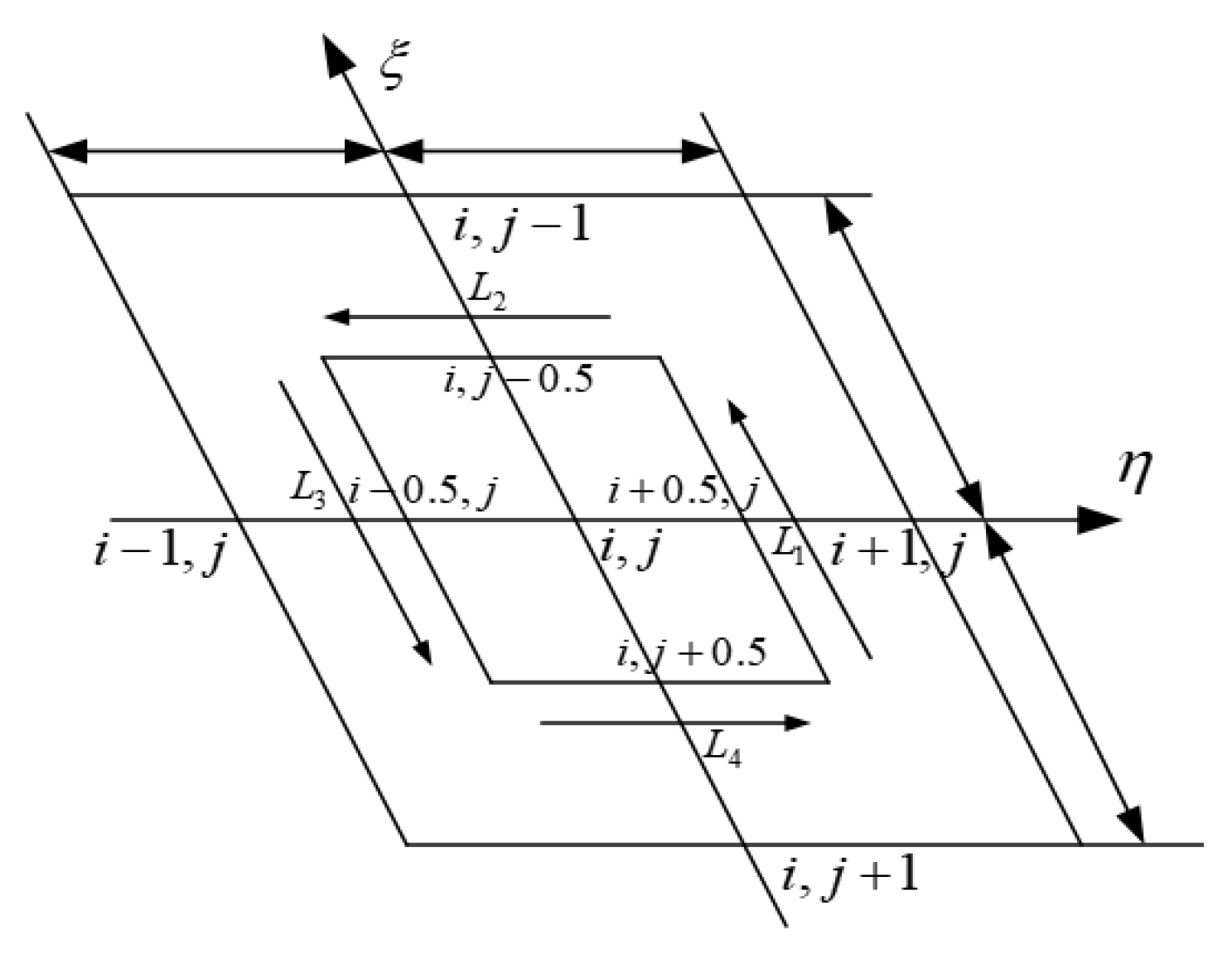
The previous derivation of the Reynolds equation is in the Cartesian coordinate system. If the rectangular grid is divided according to the ordinary bearing during the difference calculation, the boundary error will be large. Therefore, coordinate transformation is required. The calculation is carried out in the oblique coordinate system consistent with the direction of the grooves. Figure 2 below is a schematic diagram of coordinate conversion:

As shown in Figure 2, to convert the Cartesian coordinate system to the oblique coordinate system, the corresponding calculation formula is:

$$\{\begin{array}{l}\phi =\eta -\xi \cos \alpha \\ \lambda =\xi \sin \alpha \end{array}\iff \{\begin{array}{l}\eta =\phi +\lambda \tan \alpha \\ \xi =\lambda /\sin \alpha \end{array}$$

(11)

Then the expression of the partial derivative of pressure with respect to the coordinate axis direction in the Reynolds equation can be obtained:

$$\{\begin{array}{l}\frac{\partial p}{\partial \phi }=\frac{\partial p}{\partial \eta }\frac{\partial \eta }{\partial \phi }+\frac{\partial p}{\partial \xi }\frac{\partial \xi }{\partial \phi }=\frac{\partial p}{\partial \eta }\\ \frac{\partial p}{\partial \lambda }=\frac{\partial p}{\partial \eta }\frac{\partial \eta }{\partial \lambda }+\frac{\partial p}{\partial \xi }\frac{\partial \xi }{\partial \lambda }=1/\tan \alpha \frac{\partial p}{\partial \eta }+1/\sin \alpha \frac{\partial p}{\partial \xi }\\ \frac{\partial H}{\partial \phi }=\frac{\partial H}{\partial \eta }\end{array}$$

(12)

Substitute Formula (12) into the Reynolds equation in the Cartesian coordinate system and organize the static Reynolds equation in the oblique coordinate system as:

$$\left(1+\frac{d^2}{b^2{\tan }^2\alpha }\right)\frac{\partial }{\partial \eta }\left(\frac{H^3}{k_x}\frac{\partial p}{\partial \eta }\right)+\frac{d^2}{b^2{\sin }^2\alpha }\frac{\partial }{\partial \xi }\left(\frac{H^3}{k_z}\frac{\partial p}{\partial \xi }\right)+\frac{d^2}{b^2\tan \alpha \sin \alpha }\left[\frac{\partial }{\partial \eta }\left(\frac{H^3}{k_x}\frac{\partial p}{\partial \xi }\right)+\frac{\partial }{\partial \xi }\left(\frac{H^3}{k_z}\frac{\partial p}{\partial \eta }\right)\right]=\frac{1}{4}\frac{\partial H}{\partial \eta }$$

(13)

The dynamic Reynolds equation in the oblique coordinate system is obtained in the same way.

2.2.2. Static Reynolds Equation II

When dividing the mesh, the mesh boundary should coincide with the bearing ridge and groove boundary, so that the calculation accuracy is higher, and so the mesh shape is a parallelogram. Figure 3 shows that there are positions where the film thickness has a step change, which is difficult to calculate. At the same time, there is a cross partial derivative term in the equation where the film thickness is continuous, so the previous five-point difference method is no longer applicable. In this paper, the local integration method is used to study the continuous area of the oil film thickness and the step change of the oil film thickness to explain the principle of solving the equation.

(1)

Continuous area of the oil film thickness:

For areas A and D, the oil film thickness is continuous. The integral area of the node $\left(i,j\right)$ where the film thickness is continuous is the small parallelogram region in the middle of the Figure 4.

Integrate both sides of the static Reynolds equation at the same time [5]:

$${\displaystyle \underset{D_{i,j}}{\iint }\left[\frac{\partial }{\partial \phi }\left(\frac{H^3}{k_x}\frac{\partial p}{\partial \phi }\right)+{\left(\frac{d}{b}\right)}^2\frac{\partial }{\partial \lambda }\left(\frac{H^3}{k_z}\frac{\partial p}{\partial \lambda }\right)\right]}d\phi d\lambda =\frac{1}{4}{\displaystyle \underset{D_{i,j}}{\iint }\left(\frac{\partial H}{\partial \phi }\right)}d\phi d\lambda$$

(14)

Use Green’s formula to convert to line integral form:

$${\displaystyle \underset{L_{i,j}}{\int }\frac{H^3}{k_x}\frac{\partial p}{\partial \phi }}d\lambda -{\left(\frac{d}{b}\right)}^2{\displaystyle \underset{L_{i,j}}{\int }\frac{H^3}{k_z}\frac{\partial p}{\partial \lambda }}d\phi =\frac{1}{4}{\displaystyle \underset{L_{i,j}}{\int }H}d\lambda$$

(15)

Substitute the coordinate transformation Expression (11) and the pressure deviation Expression (12) into the above formula, and the five-point difference formula of the oil film continuum area under the oblique coordinates can be obtained as follows:

$$P_{i,j}=\frac{A_{i,j}{P}_{i+1,j}+B_{i,j}{P}_{i-1,j}+C_{i,j}{P}_{i,j+1}+D_{i,j}{P}_{i,j-1}-F_{i,j}}{E_{i,j}}$$

(16)

In the formula:

$$A_{i,j}=\frac{\Delta \xi }{\Delta \eta }\sin \alpha \frac{H_{i+0.5,j}^3}{k_x}-{\left(\frac{d}{b}\right)}^2\left(\frac{-H_{i,j-0.5}^3+H_{i,j+0.5}^3}{2k_z\tan \alpha }-\frac{\Delta \xi }{\Delta \eta }\frac{\cos \alpha }{\tan \alpha }\frac{H_{i+0.5,j}^3}{k_z}\right)$$

$$B_{i,j}=\frac{\Delta \xi }{\Delta \eta }\sin \alpha \frac{H_{i-0.5,j}^3}{k_x}-{\left(\frac{d}{b}\right)}^2\left(\frac{H_{i,j-0.5}^3-H_{i,j+0.5}^3}{2k_z\tan \alpha }-\frac{\Delta \xi }{\Delta \eta }\frac{\cos \alpha }{\tan \alpha }\frac{H_{i-0.5,j}^3}{k_z}\right)$$

$$C_{i,j}=-{\left(\frac{d}{b}\right)}^2\left(-\frac{\Delta \eta }{\Delta \xi }\frac{1}{\sin \alpha }\frac{H_{i,j+0.5}^3}{k_z}-\cos \alpha \frac{-H_{i+0.5,j}^3+H_{i-0.5,j}^3}{2k_z\sin \alpha }\right)$$

$$D_{i,j}=-{\left(\frac{d}{b}\right)}^2\left(-\frac{\Delta \eta }{\Delta \xi }\frac{1}{\sin \alpha }\frac{H_{i,j-0.5}^3}{k_z}-\cos \alpha \frac{H_{i+0.5,j}^3-H_{i-0.5,j}^3}{2k_z\sin \alpha }\right)$$

$$E_{i,j}=A_{i,j}+B_{i,j}+C_{i,j}+D_{i,j}$$

$$F_{i,j}=\frac{1}{4}\sin \alpha \Delta \xi \left(H_{i+0.5,j}-H_{i-0.5,j}\right)$$

(2)

Noncontinuous area of the oil film thickness:

For the noncontinuous area of the oil film thickness, such as area B, the node falls on the boundary between the ridge and the groove, and the film thickness has a step change, as shown in Figure 5. Integrate the areas on both sides of the node $\left(i,j\right)$ separately, and use the same processing method as the continuous area of the oil film thickness. The five-point difference formula of the oil film discontinuous area under the oblique coordinate is as follows:

$$P_{i,j}=\frac{A_{i,j}^{\prime }{P}_{i+1,j}+B_{i,j}^{\prime }{P}_{i-1,j}+C_{i,j}^{\prime }{P}_{i,j+1}+D_{i,j}^{\prime }{P}_{i,j-1}-F_{i,j}^{\prime }}{E_{i,j}^{\prime }}$$

(17)

In the formula:

$$A_{i,j}^{\prime }=\frac{\Delta \xi }{\Delta \eta }\sin \alpha \frac{H_{i+0.5,j}^3}{k_x}-{\left(\frac{d}{b}\right)}^2\left(\frac{-H_1^3-H_2^3+H_3^3+H_4^3}{2k_z\tan \alpha }-\frac{\Delta \xi }{\Delta \eta }\frac{\cos \alpha }{\tan \alpha }\frac{H_{i+0.5,j}^3}{k_z}\right)$$

$$B_{i,j}^{\prime }=\frac{\Delta \xi }{\Delta \eta }\sin \alpha \frac{H_{i-0.5,j}^3}{k_x}-{\left(\frac{d}{b}\right)}^2\left(\frac{H_1^3+H_2^3-H_3^3-H_4^3}{2k_z\tan \alpha }-\frac{\Delta \xi }{\Delta \eta }\frac{\cos \alpha }{\tan \alpha }\frac{H_{i-0.5,j}^3}{k_z}\right)$$

$$C_{i,j}^{\prime }=-{\left(\frac{d}{b}\right)}^2\left(-\frac{\Delta \eta }{\Delta \xi }\frac{1}{\sin \alpha }\frac{H_3^3+H_4^3}{k_z}-\cos \alpha \frac{-H_{i+0.5,j}^3+H_{i-0.5,j}^3}{2k_z\sin \alpha }\right)$$

$$D_{i,j}^{\prime }=-{\left(\frac{d}{b}\right)}^2\left(-\frac{\Delta \eta }{\Delta \xi }\frac{1}{\sin \alpha }\frac{H_1^3+H_2^3}{k_z}-\cos \alpha \frac{H_{i+0.5,j}^3-H_{i-0.5,j}^3}{2k_z\sin \alpha }\right)$$

$$E_{i,j}^{\prime }=A_{i,j}^{\prime }+B_{i,j}^{\prime }+C_{i,j}^{\prime }+D_{i,j}^{\prime }$$

$$F_{i,j}^{\prime }=\frac{1}{4}\sin \alpha \Delta \xi \left(H_{i+0.5,j}-H_{i-0.5,j}\right)$$

2.3. Boundary Conditions and Convergence Criteria

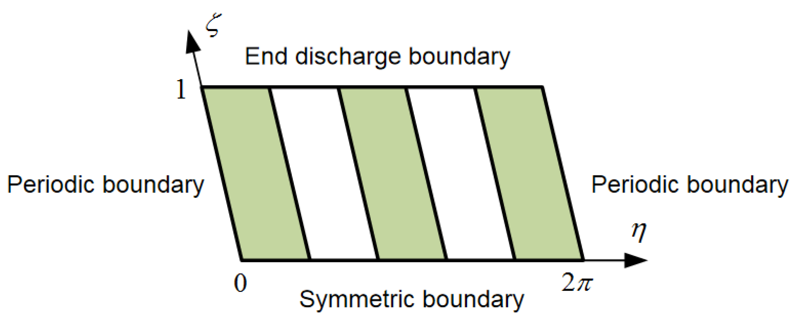
The schematic diagram of the boundary of the herringbone grooved journal bearing is shown in Figure 6. The static Reynolds equation of the HGJBs adopts Reynolds boundary conditions, namely:

$$\{\begin{array}{l}\mathrm{Side} \mathrm{boundary}:P{|}_{\xi =\pm 1/\sin \alpha }=0\\ \mathrm{Periodic} \mathrm{boundary}:P_{\eta =0}=P_{\eta =2\pi }\\ \mathrm{Reynolds} \mathrm{boundary}:P{|}_{\eta \ge {\eta }_1}=0;\frac{\partial P}{\partial \eta }{|}_{\eta \ge {\eta }_1}=0\end{array}$$

(18)

For the boundary conditions of the dynamic Reynolds equation, the disturbance pressure is 0.

In order to facilitate the calculation, the static Reynolds equation is discretized by the finite difference method, that is, the derivative form is expressed in the form of a difference quotient. In order to make the convergence faster, the over-relaxation iteration method is used to obtain the pressure of each iteration, and the iteration can be stopped when the convergence condition in the following formula is met.

$$\frac{{\displaystyle {\sum }_{j=2}^n{\displaystyle {\sum }_{i=2}^m\left|P_{i,j}^{\left(k\right)}-P_{i,j}^{\left(k-1\right)}\right|}}}{{\displaystyle {\sum }_{j=2}^n{\displaystyle {\sum }_{i=2}^m\left|P_{i,j}^{\left(k\right)}\right|}}}\le {10}^{-4}$$

(19)

$P_{i,j}^k$ represents the iteration of oil film pressure.

Since the dynamic Reynolds equation is similar in form to the static Reynolds equation, the finite difference method is also used to solve the dynamic Reynolds equation. After the convergence condition is met, the iteration is stopped.

The convergence condition of the deflection angle is:

$$\left|{\overline{F}}_x/{\overline{F}}_y\right|\le {10}^{-4}$$

(20)

2.4. Performance Calculation of HGJBs

The dimensionless horizontal and vertical load capacities of the bearings are:

$${\overline{F}}_x={\displaystyle {\int }_0^{2\pi }\left({\displaystyle {\int }_{-1}^{1}Pd\lambda }\right)\sin \phi d\phi }$$

$${\overline{F}}_y={\displaystyle {\int }_0^{2\pi }\left({\displaystyle {\int }_{-1}^{1}Pd\lambda }\right)\cos \phi d\phi }$$

(21)

The actual load capacity of the bearing is:

$$F=\frac{\omega r^3\mu l}{c^2}\sqrt{{\overline{F}}_x^2+{\overline{F}}_y^2}$$

(22)

The bearing deflection angle is:

$${\theta }_i={\theta }_{i-1}-\arctan \left|{\overline{F}}_x/{\overline{F}}_y\right|$$

(23)

The side leakage is:

$$Q_L=-4cul\left[\left(\frac{r^2}{l^2}\frac{H^3}{k_z}\frac{\partial p}{\partial \lambda }{|}_{\lambda =1}\right)-\left(\frac{r^2}{l^2}\frac{H^3}{k_z}\frac{\partial p}{\partial \lambda }{|}_{\lambda =-1}\right)\right]d\phi$$

(24)

The bearing friction resistance is:

$$F_t=\frac{\omega r^2\mu l}{2c}{\displaystyle \iint \left(\frac{1}{H}{\tau }_c-\frac{12H}{k_x}\frac{\partial p}{\partial \phi }\right)}d\phi d\lambda$$

(25)

In the formula: ${\tau }_c$ is the Coot shear stress.

The bearing friction power is:

$$N_t=F_t\cdot U$$

(26)

The average temperature rise of the bearing is:

$$\Delta T=\frac{F_{t}U}{Q_L\rho c_v}$$

(27)

When the axis only makes small movements near the static equilibrium position, eight linearized stiffness and damping coefficients can be used to express the dynamic performance of the oil film:

$$\left\{\begin{array}{l}{K}_{ee}\\ K_{\theta e}\end{array}\right\}=-{\displaystyle {\int }_{-1}^1{\displaystyle {\int }_{{\phi }_1}^{{\phi }_2}{P}_{\epsilon }\left\{\begin{array}{l}\cos \phi \\ \sin \phi \end{array}\right\}}}d\phi d\lambda$$

(28)

$$\left\{\begin{array}{l}{K}_{e\theta }\\ K_{\theta \theta }\end{array}\right\}=-{\displaystyle {\int }_{-1}^1{\displaystyle {\int }_{{\phi }_1}^{{\phi }_2}{P}_{\theta }\left\{\begin{array}{l}\cos \phi \\ \sin \phi \end{array}\right\}}}d\phi d\lambda$$

(29)

$$\left\{\begin{array}{l}{D}_{ee}\\ D_{\theta e}\end{array}\right\}=-{\displaystyle {\int }_{-1}^1{\displaystyle {\int }_{{\phi }_1}^{{\phi }_2}{P}_{{\epsilon }^{\prime }}\left\{\begin{array}{l}\cos \phi \\ \sin \phi \end{array}\right\}}}d\phi d\lambda$$

(30)

$$\left\{\begin{array}{l}{D}_{e\theta }\\ D_{\theta \theta }\end{array}\right\}=-{\displaystyle {\int }_{-1}^1{\displaystyle {\int }_{{\phi }_1}^{{\phi }_2}{P}_{{\theta }^{\prime }}\left\{\begin{array}{l}\cos \phi \\ \sin \phi \end{array}\right\}}}d\phi d\lambda$$

(31)

Therefore, in the specific calculation, first of all, we must divide the grid, given the basic parameters of the bearing, initialize the oil film pressure, and obtain the convergent oil film pressure by iterating the oil film pressure and correcting the deflection angle. Then calculate the static and dynamic performance of the bearing. The whole calculation process is carried out in the Matlab software. The specific program flow chart is shown in Figure 7.

2.5. Verification of HGJBs Program

In order to verify the correctness of the calculation program for HGJBs, this paper used the parameters of the journal bearing in the references to calculate the oil film pressure of the bearing and compared it with the experimental values in reference [38] and the theoretical values in reference [39] to verify the correctness of the calculation model in this paper. The comparison diagram is shown in Figure 8.

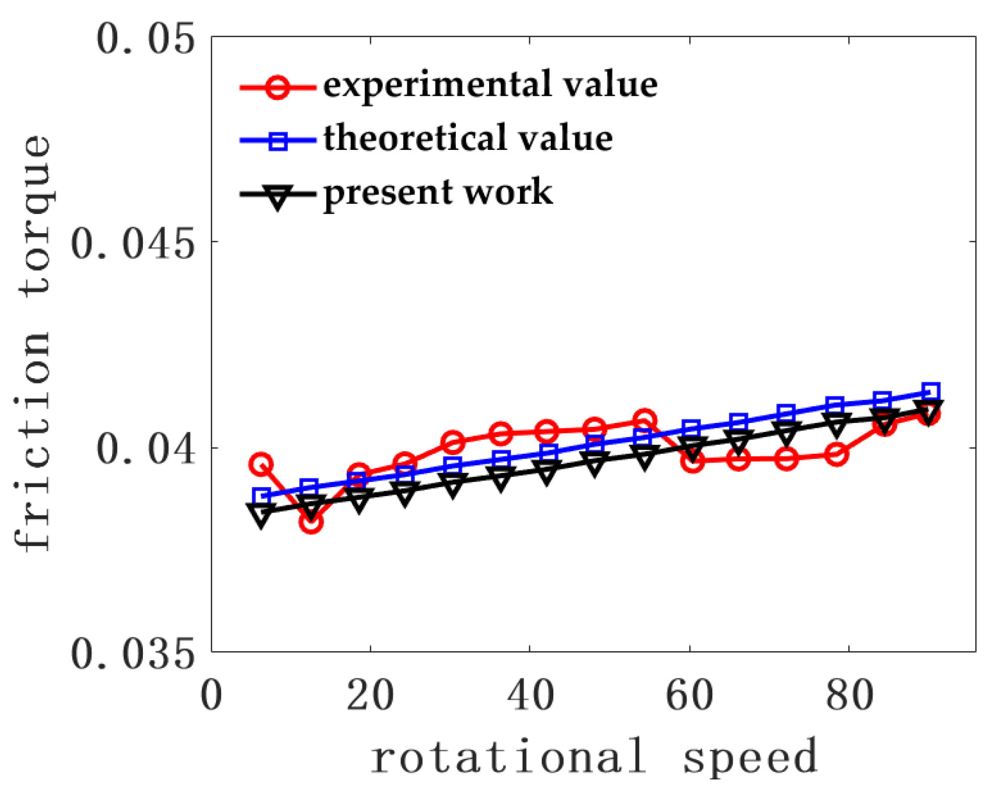
At the same time, we used the parameters of the herringbone groove journal bearing in the reference to calculate the friction torque of the bearing and compared it with the experimental and theoretical results in the reference [40] to verify the correctness of the calculation model in this paper. The comparison diagram is shown in Figure 9.

The Figure 8 and Figure 9 show that the numerical calculation in this paper has the same distribution trend as the results in the references. Therefore, it is quantitatively verified that the bearing static and dynamic performance calculation results obtained by the MATLAB calculation program in this paper are correct.

When using the finite difference method to solve the bearing performance, the mesh density is the key to ensuring the accuracy of the calculation results. In order to determine the reasonable number of grids, a variety of differential grid numbers were used to calculate the bearing capacity of the herringbone groove journal bearing. The results can be seen in the Figure 10. Finally, the reasonable number of grids is determined to be 280 × 200, and the calculation result is not much different from 350 × 360.

3. Results

The parameters of the HGJBs and lubricants used in the following calculation and analysis are shown in

Table 1. Calculation parameters of HGJBs and lubricants.

Parameter	Numerical Value
$\mathrm{Bearing} \mathrm{diameter} \mathrm{d}/\mathrm{mm}$	30
$\mathrm{Width} \mathrm{to} \mathrm{diameter} \mathrm{ratio} L/d$	1
$\mathrm{Radius} \mathrm{gap} \mathrm{c}/\mathrm{mm}$	0.02
$\mathrm{Lubricant} \mathrm{viscosity} \mathsf{\mu }/(\mathrm{pa}·\mathrm{s}$)	$8.63\times {10}^{-4}$
$\mathrm{Rotation} \mathrm{rate} \mathrm{N}/\left(\mathrm{r}·{\min }^{-1}\right)$	10,000
Number of grooves $\mathrm{n}$	10
Groove depth	0.02
Groove to ridge ratio	1
Helix angle $\alpha$/°	30
Convergence angle β/°	25

.

3.1. Comparison of the Turbulence Flow Model and the Laminar Flow Model

In fluid mechanics, the motion state of fluid is divided into the laminar motion state and turbulence motion state. The critical Reynolds number usually is used to distinguish these two states. The critical Reynolds number formula is as follows:

$$R_e=\frac{\rho vh}{\mu }$$

(32)

In the formula, $\rho$ is the density of the fluid. $v$ is the tangential relative velocity of the relative moving surface. $h$ is the oil film thickness of the journal bearing, and $\mu$ is the dynamic viscosity of the lubricant.

When the bearing is running at low speed, its lubricating medium is mainly laminar flow, and the flow state coefficient is constant. Since this study is aimed at the herringbone groove journal bearing in the CT tube, the supporting speed reaches 10,000 rpm, the lubricating medium is liquid metal, and the viscosity is very low, about twice the viscosity of water at room temperature, so a comprehensive turbulence lubrication model is adopted.

Figure 11 shows the comparison of the turbulence flow model and the laminar flow model. After considering the turbulence flow state, the fluid molecules move violently. Compared with the laminar flow model, the bearing load capacity, side leakage, and friction power become larger, and the average temperature rise becomes smaller.

3.2. Comparison of Cartesian Coordinate System and Oblique Coordinate System

Figure 12 below shows the oil film thickness diagram and pressure distribution diagram of the constant-width HGJBs calculated using the Cartesian coordinate system and the oblique coordinate system when the eccentricity is 0.4, where Figure 12a,b are the calculation results using the Cartesian coordinate system, and Figure 12c,d are the calculation results using the oblique coordinate system:

Figure 12 shows that the overall trend of the oil film thickness and the pressure distribution are consistent in the rectangular coordinate system and the oblique coordinate system. However, the pressure distribution of HGJBs in the oblique coordinate system is smoother, and the direction is consistent with the boundary of the herringbone groove shape, and the iteration direction is more in line with the supporting principle of HGJBs and closer to the flow direction of the lubricating medium. Therefore, the calculation using the oblique coordinate system can better reflect the real situation of the bearing work, and the calculation accuracy is higher.

3.3. Oil Film Thickness and Pressure Distribution of Different Structures

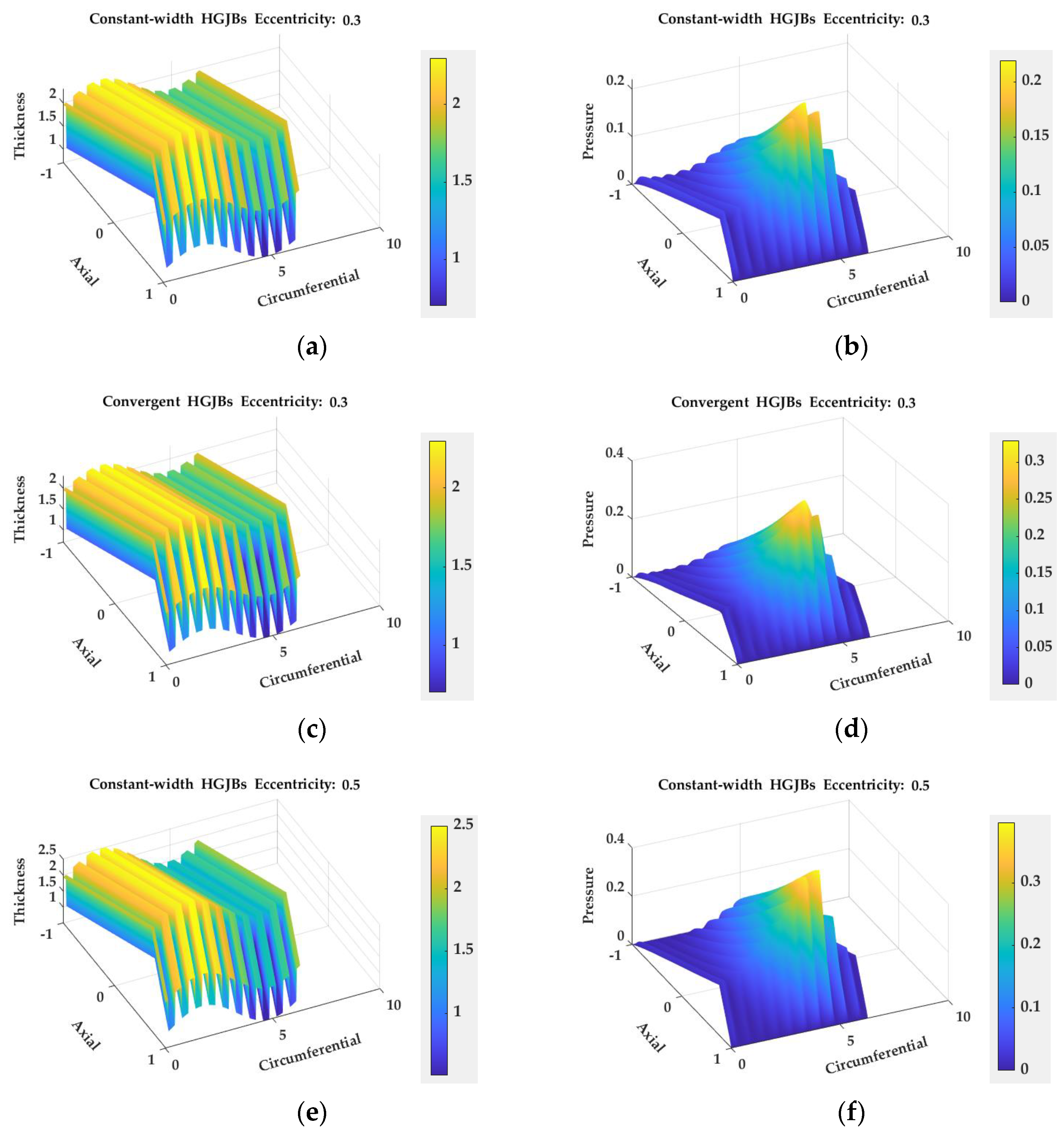
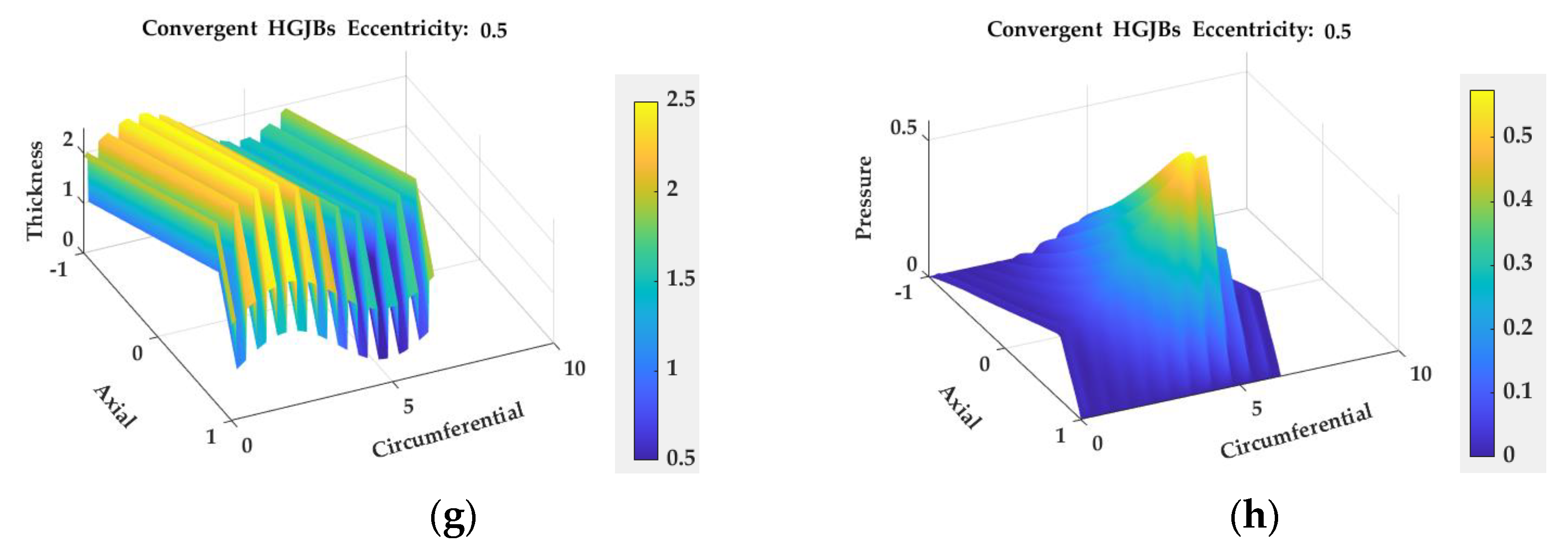
Figure 13 shows the oil film thickness diagram and pressure distribution diagram of the constant-width HGJBs and the newly designed convergent HGJBs calculated using the oblique coordinate system when the eccentricity is 0.3 and 0.5, where Figure 13a,b,e,f are the calculation results of the constant-width HGJBs, and Figure 13c,d,g,h are the calculation results of the convergent HGJBs.

Figure 13 shows that due to the presence of herringbone grooves, the oil film of HGJBs is distributed in steps, which can be divided into groove areas and ridge areas along the circumferential direction. Assuming that the herringbone groove is set on the shaft and the corresponding bearing bush is smooth, the shaft rotates at a certain speed and pumps the liquid on one side of the bearing. This phenomenon is called the pumping effect. Therefore, the pressure distribution diagram shows that the pressure of the HGJBs is distributed in a zigzag shape in the circumferential direction, and each groove will have a pressure peak. The pumping effect formed by the unique structure of the herringbone groove itself makes the pressure in the groove greater at the center of the herringbone groove, and the peak of the oil film pressure appears at the top of the herringbone groove. Since the herringbone pressure belt is encircled on the journal, the bearing can load in all directions, thereby improving the vibration resistance and stability of the bearing.

The groove width of the constant-width HGJBs is equal everywhere, while the groove structure of the convergent HGJBs is convergent. The difference between the two can be well seen through the oil film thickness distribution diagram. Under small eccentricity, there is little difference in oil film pressure between the two. Under large eccentricity, there is a big difference in oil film pressure between the two. The oil film pressure of the convergent HGJBs is greater than that of the constant-width HGJBs.

3.4. Performance Comparison of Bearings with Different Structures

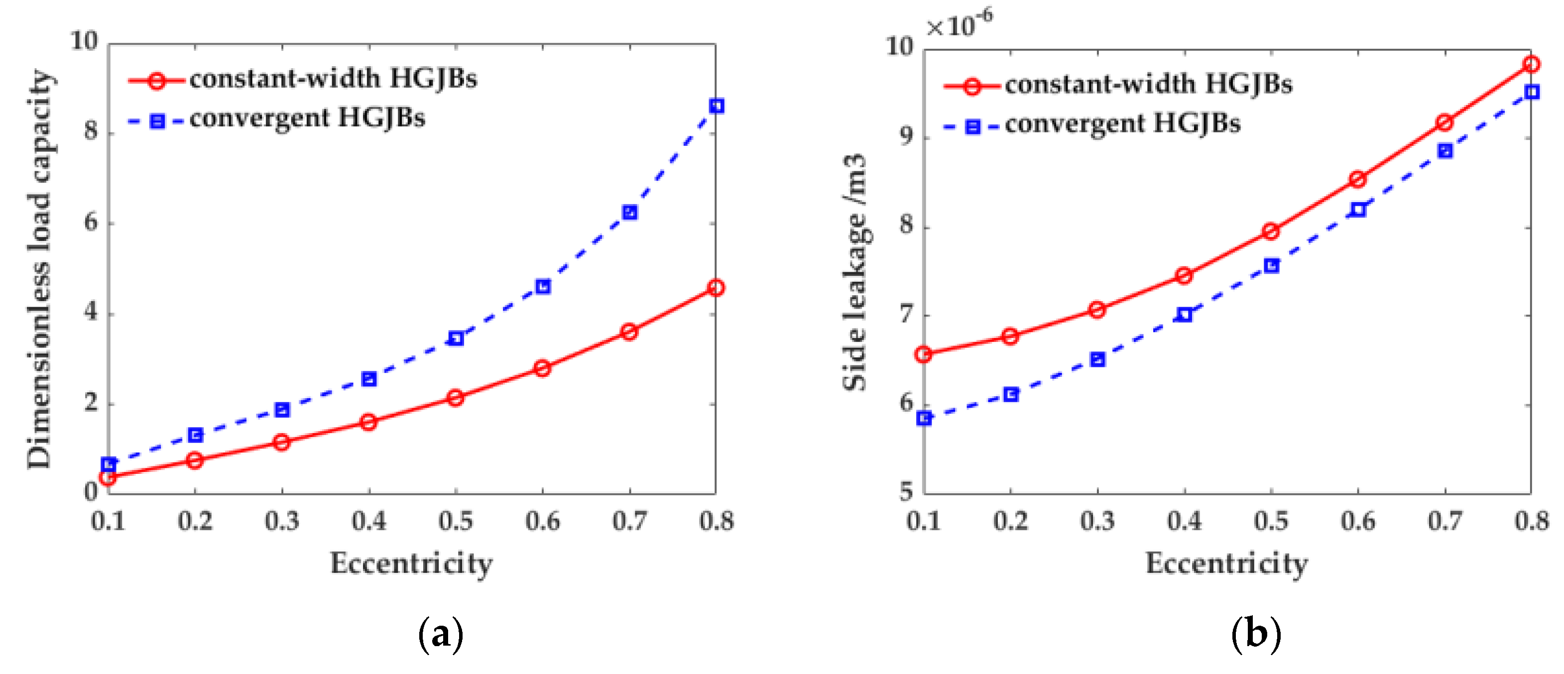
We kept other parameters unchanged, changed the eccentricity from 0.1 to 0.8, and analyzed the changes in the static and dynamic performance of the convergent HGJBs and constant-width HGJBs, as shown in Figure 14.

Figure 14 shows that the bearing load capacity increases with the increase of eccentricity. Increasing the eccentricity makes the minimum oil film thickness of the bearing smaller, and the wedge effect is more significant, so the bearing load capacity increases. Under large eccentricity, the oil film thickness is of smaller order of magnitude. As the eccentricity increases, a smaller thickness change will have a greater impact on the oil film pressure. When the eccentricity changes from 0.6 to 0.8, the bearing load capacity of the convergent HGJBs increases by 86.25%. Since the groove of the convergent HGJBs also changes in the width direction, the lubricating oil flows from the wide port to the narrow port, resulting in a greater wedge effect. Under small eccentricity, the bearing load capacity difference between convergent HGJBs and constant-width HGJBs is small, and under large eccentricity, the performance difference between the two is larger. When the eccentricity is 0.8, the bearing load capacity of the convergent HGJBs is 87.76% larger than that of the constant-width HGJBs.

With the increase of eccentricity, the minimum oil film thickness decreases, and the pressure gradient increases, which leads to an increase in bearing side leakage. The friction power increases with the increase of eccentricity, so that the average temperature rise of the bearing also increases. Compared with the constant-width HGJBs, the groove shape of the convergent HGJBs is in a convergent state, resulting in a smaller herringbone groove area and a smaller overall oil film thickness. Therefore, its lubricating oil reserve is less, resulting in convergent HGJBs having smaller side leakage and greater friction power resistance. When the eccentricity is 0.5, the side leakage is 4.83% smaller than that of the constant-width HGJBs, which causes the average temperature rise to increase. But it can be seen from the Figure 11 that there is not much difference between the side leakage and the average temperature rise between the both.

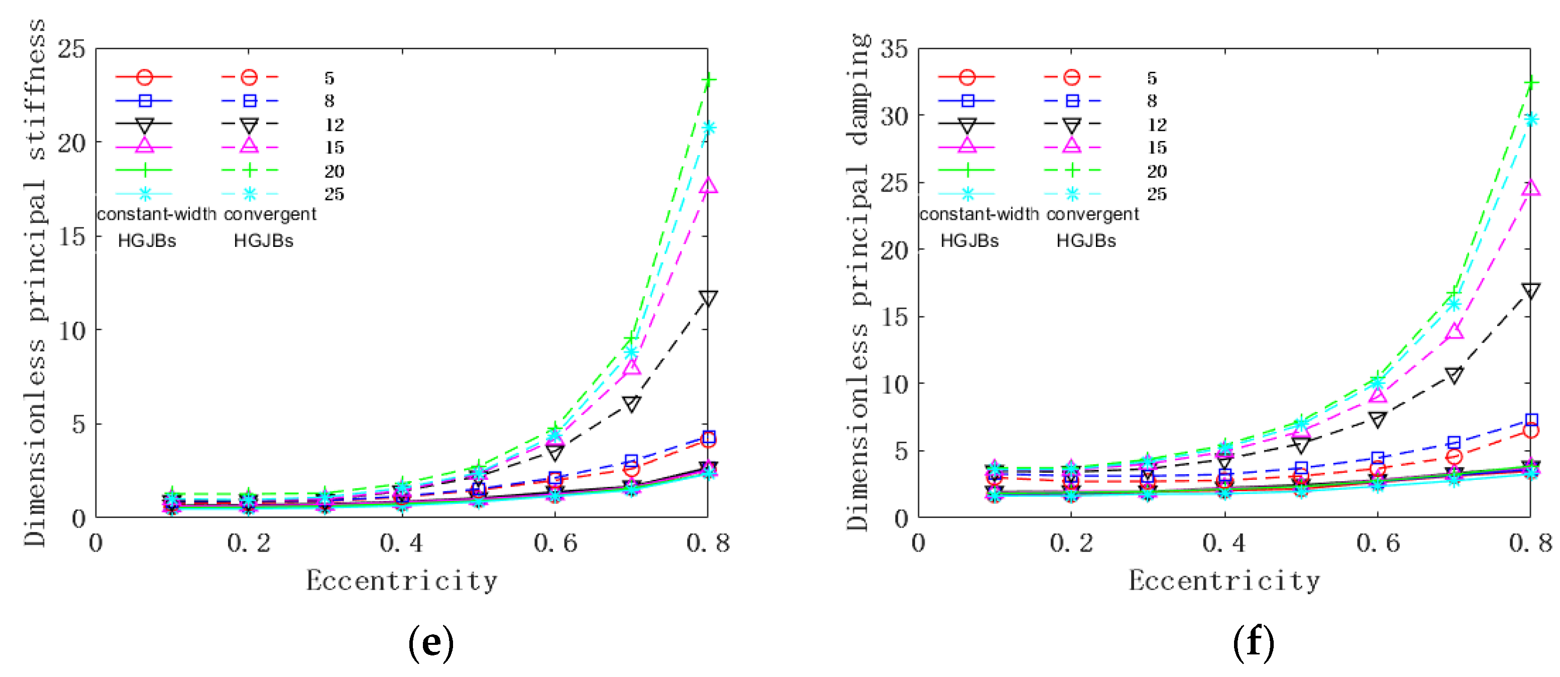
Stiffness and damping coefficients are important indicators to measure the stability of the bearing. With the increase of eccentricity, the stiffness and damping coefficients of the bearing basically keep increasing. When the eccentricity is small, the increase is slower, and when the eccentricity is large, the increase in the stiffness and damping coefficients is larger in both. Compared with the constant-width HGJBs, the convergent HGJBs has larger stiffness and damping coefficients. When the eccentricity is 0.8, the stiffness of the convergent HGJBs is about four times that of the constant-width HGJBs. Therefore, the optimized convergent HGJBs has larger load capacity and dynamic performance. Although the temperature rise has increased, the amplitude is not large and belongs to the controllable range.

3.5. The Influence of the Number of Grooves on the Performance of HGJBs

The number of grooves has a direct effect on the amount of lubricating oil storage, the number of pumping effects and step effects, and the stiffness of the bearings. We kept other parameters unchanged, took the number of grooves as 5, 8, 12, 15, 20, and 25; and analyzed the influence of the number of grooves on the performance of bearings with different structures as shown in Figure 15.

Figure 15 shows that when the number of grooves is small, as the number of grooves increases, the bearing load capacity of the oil film gradually increases. This is because when the number of grooves is small, the stepped dynamic pressure effect of the bearing is smaller, so the bearing load capacity is small; when the number of grooves gradually increases, the stepped dynamic pressure effect increases, so the bearing load capacity gradually increases. When the number of grooves is large, the pumping effect of the bearing reaches saturation, and the bearing load capacity remains basically unchanged at this time. When the number of grooves is 20, the bearing load capacity of the constant-width HGJBs reaches the maximum. Since the wedge effect is more pronounced in convergent HGJBs, the number of grooves corresponding to its maximum bearing load capacity is larger. The calculated number of grooves corresponding to the maximum bearing load capacity of the convergent HGJBs is 30. With the increase in the number of grooves, the bearing side leakage and friction power also show an increasing trend, and the average temperature rise of the bearing gradually decreases and tends to be flat. But the changes are not big. When the eccentricity is 0.5, the maximum friction power of the convergent HGJBs is 6.43% larger than the minimum friction power, and the maximum friction power of the constant-width HGJBs is 0.12% larger than the minimum friction power. In terms of friction, the number of grooves has a more significant influence on the convergent HGJBs.

As the number of grooves increases, the stiffness and damping coefficients of the two bearings first increase and then gradually decrease. The larger the number of grooves, the faster the stiffness coefficient and damping coefficient decrease. This is because when the number of grooves is small, the pressure is relatively concentrated, and there is basically only one peak point. The pressure distribution before and after the peak point decreases sharply, and the stability is poor; when there are more grooves, the width of the ridge decreases, and the excessive shear stress of the local groove root causes the stiffness coefficient to decrease. At the same time, due to the pumping effect, the bearing pressure distribution is more concentrated, and the pressure distribution range is small, and the stability is worse. Compared with constant-width HGJBs, the stiffness and damping coefficients of convergent HGJBs are much larger. When the number of grooves is 20, the stiffness coefficient and damping coefficient of the convergent HGJBs are the largest. Because an increase in the number of grooves will increase the difficulty and cost of bearing processing, it is recommended that the number of convergent HGJBs be 15–20 and the number of constant-width HGJBs be 8–12 within the allowable range of processing.

3.6. The Influence of Helix Angle on the Performance of HGJBs

The helix angle has a direct effect on the direction of the lubricating oil flow in the HGJBs. We kept other parameters unchanged, took the helix angle as 15°, 30°, 45°, 60°, and 75°; and analyzed the influence of the helix angle on the performance of bearings with different structures as shown in Figure 16.

Figure 16 shows that as the helix angle increases, the bearing load capacity of the bearing gradually increases to the maximum value and then decreases rapidly at a faster rate. It shows that as the helix angle gradually increases, the pumping effect of the bearing increases, so the bearing load capacity gradually increases. When it is increased to a certain range, the pumping effect is the best, and then the bearing load capacity gradually decreases. The Figure 16 shows that the helix angle has a more obvious influence on the bearing load capacity of the convergent HGJBs than that of the constant-width HGJBs. When the helix angle is 30°, the pumping effect of the convergent HGJBs reaches its best result, which is nearly twice the bearing load capacity corresponding to the helix angle of 45° when the eccentricity is 0.7. Similarly, when the helix angle is 30°, the bearing load capacity of the constant-width HGJBs is the largest, and when the eccentricity is 0.5, it is only half of the maximum bearing load capacity of the convergent HGJBs. The side leakage increases with the increase of the helix angle of the HGJBs. When the helix angle is 75°, the corresponding side leakage of the convergent HGJBs is nearly five times that when the helix angle is 15°. As the helix angle increases, the friction power of the convergent HGJBs also increases, but the amount of change is not obvious, and the increase is not large. Due to the increase of the side leakage, the helix angle increases, and the temperature rise decreases. When the helix angle increases from 15° to 75°, the average temperature rise drops significantly, overall, about 5 °C.

With the increase of the helix angle, the stiffness coefficient and damping coefficient of the bearing gradually increase, and the growth rate decreases with the increase of the helix angle. When the helix angle is small, the stability of the bearing is poor. The stiffness coefficient of the convergence HGJBs basically remains stable after the helix angle of 45°. When the eccentricity is 0.5, the stiffness coefficient corresponding to the helix angle of 75° is basically the same as the stiffness coefficient corresponding to the helix angle of 45°.

Considering the bearing load capacity and stability factors, the helix angle of the convergent HGJBs is 30°–45°, and the helix angle of the constant-width HGJBs is 30°–45°. At this time, the bearing performance is the best.

3.7. The Influence of Groove to Ridge Ratio on the Performance of HGJBs

The HGJB groove to ridge ratio is the ratio of the groove width to the convex ridge width. The groove to ridge ratio will directly affect the stiffness of the bearing and the amount of lubricating oil. We kept other parameters unchanged, took the groove to ridge ratio as 0.5, 0.8, 1.0, 1.5, and 2.0; and analyzed the influence of the groove to ridge ratio on the performance of bearings with different structures, as shown in Figure 17.

Figure 17 shows that with the increase of the groove to land ratio, the bearing load capacity of the bearing gradually decreases, but the magnitude of the change is smaller relative to the influence of the number of grooves and the helix angle on the bearing load capacity. When the groove to ridge ratio is equal to 0 or infinite, the bearing surface of the bearing becomes a full table area or a full groove area, which is equivalent to an ordinary journal bearing, and the full groove area is equivalent to increasing the bearing clearance, making the bearing load capacity much smaller than the full table area. When the eccentricity is 0.5 and the groove to ridge ratio is 0.5, the bearing load capacity of the convergent HGJBs is nearly 1.6 times that of the constant-width HGJBs. The friction power decreases proportionally with the increase of the groove to ridge ratio. This is mainly because the larger the groove to ridge ratio, the larger the herringbone groove area, and the larger the overall oil film thickness, resulting in lower friction. The friction power of the convergent HGJBs is reduced by 2% every time the groove to ridge ratio increases by 0.5. With the gradual increase of the ridge to ridge ratio, the side leakage also increases and tends to a stable value, and the temperature rise gradually decreases and stabilizes. This is because increasing the groove to ridge ratio is equivalent to increasing the herringbone groove area, indirectly increasing the clearance between the bearing and the journal, and increasing the volume of stored lubricating oil; resulting in an increase in side leakage and a decrease in average temperature rise.

As the ratio of groove to ridge increases, the area of the herringbone groove increases, and the dynamic pressure effect of the oil film gradually strengthens, and the stiffness coefficient increases significantly. The Figure 17 shows that after the groove to ridge ratio of the convergent HGJBs and the constant-width HGJBs is increased to a certain extent, the oil film stiffness coefficient remains basically unchanged. When the groove to ridge ratio is 2, the overall stiffness coefficient of the convergent HGJBs is only about 3% larger than when the groove to ridge ratio is 1.5. When the eccentricity is 0.5, the maximum stiffness coefficient of the convergent HGJBs is nearly twice that of the constant-width HGJBs. With the increase of the ridge to ridge ratio, the damping coefficient also shows an increasing trend. The groove to ridge ratio makes the difference between the maximum and minimum values of the convergent HGJBs much larger than that of the constant-width HGJBs. The influence of the groove to ridge ratio on the dynamic performance of the convergent HGJBs is more obvious than that of the constant-width HGJBs.

Therefore, considering the bearing, stiffness, and rationality of design and processing, when the convergent HGJBs groove to ridge ratio is selected as 1, that is, when the groove width and the convex ridge width are equal, the balance between the bearing load capacity and the stiffness coefficient can be achieved. At the same time, when the groove to ridge ratio of the constant-width HGJBs is selected as 1, it is also more appropriate.

3.8. The Influence of Groove Depth on the Performance of HGJBs

The depth of the groove has a direct impact on the storage capacity and flow pattern of the lubricant. We kept other parameters unchanged, the radius clearance $\mathrm{c}$ was 0.02 mm, took the groove depth as 0.5$\mathrm{c}$, 0.8$\mathrm{c}$, 1.0$\mathrm{c}$, 1.5$\mathrm{c}$, and 2$\mathrm{c}$; and the influence of the groove depth on the performance of the bearings with different structures was analyzed as shown in Figure 18.

Figure 18 shows that as the groove depth increases, the bearing load capacity shows a gradual decreasing trend; the side leakage increases, and the friction power decreases slowly with the increase of the groove depth. The temperature rise gradually decreases and stabilizes. When the groove depth is 0, the HGJBs becomes an ordinary journal bearing at the moment, so the bearing load capacity will reach the maximum. On the one hand, by increasing the groove depth, the existence of the groove will destroy the continuity of the bearing oil film pressure; on the other hand, as the groove depth increases, it will cause the generation of cavities, resulting in a decrease in the bearing load capacity. When the eccentricity is 0.5, the maximum bearing load capacity of the convergent HGJBs is 26.43% larger than the minimum bearing load capacity, and the maximum friction power is 3.06% larger than the minimum friction power. The maximum bearing load capacity of constant-width HGJBs is nearly twice as large as the minimum bearing load capacity, and the maximum friction power is 6.8% larger than the minimum friction power. The depth of the groove has a significant effect on the bearing load capacity but not on the friction power.

When the depth of the groove is small, according to Newton’s law of shear, the shear force of the lubricating oil will become larger, and the dynamic pressure effect of the bearing will be significant at this time. As the groove depth increases, the stiffness coefficient gradually decreases. When the groove depth is small, the stiffness coefficient and damping coefficient decrease quickly, which shows that it is more sensitive to the change of groove depth. As the groove depth increases, the damping coefficient basically shows a linear decreasing trend. When the eccentricity is 0.5 and the groove depth is 0.5$\mathrm{c}$, the stiffness coefficient of the convergent HGJBs is 65.16% larger than that when the groove depth is 2.0$\mathrm{c}$.

Considering factors, such as bearing load capacity and temperature rise and stiffness, the groove depth of the convergent HGJBs should not be too large, otherwise the bearing load capacity and stiffness will be poor; it should not be too small, otherwise the temperature rise will be too large. Therefore, the groove depth can be selected to be between 1.0$\mathrm{c} –$1.2$\mathrm{c}$. For constant-width HGJBs, the groove depth can be selected to be between 1.0$\mathrm{c} –$1.2$\mathrm{c}$.

4. Conclusions

Aiming at high load capacity, high stiffness, and good stability performance, the static and dynamic performance and optimization of the structure parameters of constant-width HGJBs and convergent HGJBs with liquid metal lubrication under a high temperature environment are researched in this paper. Using the finite difference method under oblique coordinate system, we systematically studied the advantages of convergent HGJBs and the influence of bearing structure parameters on the static and dynamic performance of the bearing. The work provides the thinking and reference basis for the design of liquid metal bearings of the high-performance CT device. The main conclusions are as follows:

• The HGJBs bear the load by the wedge effect and the pumping effect. Because the herringbone pressure belt is wrapped around the journal, the bearing can load in all directions, which makes its stability higher.
• The paper researched the performance of HGJBs under different eccentricity. We found that the convergent HGJBs are better than the constant-width HGJBs in terms of bearing load capacity, stiffness, and stability. Although the temperature rise increased, the amplitude was not large and belonged to the controllable range.
• With the goal of high load capacity, stiffness, and good stability, the influence of the bearing structural parameters on the performance of HGJBs was analyzed. The bearing structure parameters have a more significant influence on the performance of the convergent HGJBs. The convergent HGJBs can obtain good static and dynamic performance when the number of grooves is 15–20, the helix angle is 30°–45°, the ratio of groove-ridge is 1, and the groove depth is 0.02 mm –0.024 mm.

References

- Sun, W. The development and technical characteristics of CT imaging technology. J. Chin. Med. Device 2007, 20, 19–20. [Google Scholar]
- Shi, L.; Zhang, F.; Wang, R.; Wang, Y. Domestic and foreign situation and development trend of medical CT X-Ray tubes. Vac. Electron. 2018, 2, 61–68. [Google Scholar]
- Hattori, H.; Fukushima, H.; Yoshii, Y.; Nakamuta, H.; Iwase, M.; Kitade, K. Proposal of a high rigidity and high speed rotating mechanism using a new concept hydrodynamic bearing in X-Ray tube for high speed computed tomography. J. Adv. Mech. Des. Syst. Manuf. 2009, 3, 105–114. [Google Scholar] [CrossRef] [Green Version]
- Souchet, D.; Senouci, A.; Zaidi, H.; Amirat, M. Numerical analysis of a hydrodynamic herringbone grooved journal bearing. J. Eng. 2011, 2011, 24–27. [Google Scholar] [CrossRef]
- Zhu, H.; Ding, Q. Numerical Analysis of Static Characteristics of herringbone grooved hydrodynamic journal bearing. Appl. Mech. Mater. 2012, 105–107, 2259–2262. [Google Scholar] [CrossRef]
- Muijderman, E. Spiral groove bearings. Ind. Lubr. Tribol. 2013, 17, 12–17. [Google Scholar] [CrossRef]
- Tong, B.; Gui, C.; Sun, J.; Zhao, X.; Chen, H. Thermo-hydrodynamic lubrication analysis of internal combustion engine’s main bearing considering thermal deformation effects. Chin. J. Mech. Eng. 2007, 43, 180–185. [Google Scholar] [CrossRef]
- Lin, X.; Jiang, S.; Zhang, C.; Liu, X. Thermohydrodynamic analysis of high speed water-lubricated spiral groove thrust bearing considering effects of cavitation, inertia and turbulence. Tribol. Int. 2018, 119, 645–658. [Google Scholar] [CrossRef]
- Yang, J.; Qi, T.; Liu, B.; NI, B. Experimental study on spreading characteristics of liquid metal film under influence of magnetic field. J. Eng. Thermophys. 2017, 38, 1917–1922. [Google Scholar]
- Liu, P.; Jiang, S. Study on static characteristics of water-lubricated textured herringbone grooved journal bearings based on laminar cavitating flow lubrication model. J. Phys. Conf. Ser. 2021, 1906, 012037. [Google Scholar] [CrossRef]
- Jao, H.; Li, W.; Liu, T. Analysis of misaligned journal bearing with herringbone grooves: Consideration of anisotropic slips. Microsyst. Technol. 2017, 23, 4687–4698. [Google Scholar] [CrossRef]
- Liu, W.; Baettig, P.; Wagner, P.H.; Schiffmann, J. Nonlinear study on a rigid rotor supported by herringbone grooved gas bearings: Theory and validation. Mech. Syst. Signal Process. 2021, 146, 106983. [Google Scholar] [CrossRef]
- Eliott, G.; Jürg, S. Performance potential of gas foil thrust bearings enhanced with spiral grooves. Tribol. Int. 2019, 131, 438–445. [Google Scholar]
- Eliott, G.; Jürg, S. Dynamic force coefficients identification on air-lubricated herringbone grooved journal bearing. Mech. Syst. Signal Process. 2020, 136, 106498. [Google Scholar]
- Gu, L.; Guenat, E.; Schiffmann, J. A Review of Grooved Dynamic Gas Bearings. Appl. Mech. Rev. 2020, 72, 010801. [Google Scholar] [CrossRef]
- Hirs, G. The load capacity and stability characteristics of hydrodynamic grooved journal bearings. ASLE Trans. 1965, 8, 296–305. [Google Scholar] [CrossRef]
- Kang, K.; Rhim, Y.; Sung, K. A Study of the oil-lubricated herringbone-grooved journal bearing—Part 1: Numerical analysis. J. Tribol. 1996, 118, 906–911. [Google Scholar] [CrossRef]
- Gad, A.; Nemat-Alla, M.; Khalil, A.A.; Nasr, A. On the optimum groove geometry for herringbone grooved journal bearings. J. Tribol. 2006, 128, 585–593. [Google Scholar] [CrossRef]
- Murata, S.; Miyake, Y.; Kawabata, N. Two-dimensional analysis of herringbone grooved journal bearings. Bull. JSME 1980, 23, 1220–1227. [Google Scholar] [CrossRef]
- Bonneau, D.; Absi, J. Analysis of aerodynamic journal bearings with small number of herringbone grooves by finite element method. J. Tribol. 1994, 116, 698–704. [Google Scholar] [CrossRef]
- Li, Y.; Yang, P.; Chen, W. Design of liquid metal lubricated spiral grooved bearing considering influences of turbulence and slip. J. Xi’an Jiaotong Univ. 2019, 53, 15–23. [Google Scholar]
- Yang, P.; Chen, W. Analysis for performance herringbone spiral grooved thrust bearing. J. Xi’an Jiaotong Univ. 2020, 54, 17–27. [Google Scholar]
- Han, Y.; Wang, J.; Zhou, G.; Xiao, K.; Li, J. Micro-bottom shape effects on the misaligned herringbone grooved axial piston bearing with a new parallel algorithm. Proc. Inst. Mech. Eng. 2017, 231, 637–654. [Google Scholar] [CrossRef]
- Guo, X.; Han, Y.; Chen, R.; Wang, J.; Ni, X.; Xiao, K. A hydrodynamic lubrication model and comparative analysis for coupled microgroove journal-thrust bearings lubricated with water. Proc. Inst. Mech. Eng. Part J J. Eng. Tribol. 2020, 234, 1755–1770. [Google Scholar]
- Gao, Y.; Liu, J.; Wang, X.; Fang, Q. Investigation on the performance of gallium based liquid metal thermal interface materials. J. Eng. Thermophys. 2017, 38, 1077–1081. [Google Scholar]
- Yu, Y.; Liu, J. Technical progress and industrialization prospect of 3D liquid metal printing. J. Eng. Stud. 2017, 9, 577–585. [Google Scholar]
- Yao, F. The application of liquid metal. Sci. Technol. Vision 2019, 5, 129–131. [Google Scholar]
- Hughes, W. Magnetohydrodynamic lubrication and application to liquid metals. Ind. Lubr. Tribol. 1963, 15, 125–133. [Google Scholar] [CrossRef]
- Persad, C.; Yeoh, A. On the nature of the armature-rail interface: Liquid metal effects. IEEE Trans. Magn. 1997, 33, 140–145. [Google Scholar] [CrossRef]
- Guo, J.; Cheng, J.; Tan, H.; Zhu, S.; Qiao, Z.; Yang, J.; Liu, W. Ga-based liquid metal: A novel current-carrying lubricant. Tribol. Int. 2019, 135, 457–462. [Google Scholar] [CrossRef]
- Cheng, J.; Yu, Y.; Guo, J.; Wang, S.; Zhu, S.; Ye, Q. Ga-based liquid metal with good self-lubricity and high load-carrying capacity. Tribol. Int. 2019, 129, 1–4. [Google Scholar] [CrossRef]
- Cheng, J.; Zhu, S.; Tan, H.; Yu, Y.; Yang, J.; Li, W. Lead-bismuth liquid metal: Lubrication behaviors. Wear. 2019, 430, 67–72. [Google Scholar] [CrossRef]
- Liu, W.; Xu, J.; Feng, D.; Wang, X. Present Situation and development trend of synthetic lubricating oil. Tribology 2013, 33, 91–104. [Google Scholar]
- Li, Y.; Zhang, S.; Ding, Q.; Feng, D.; Qin, B.; Hu, L. Liquid metal as novel lubricant in a wide temperature range from −10 to 800 °C. Mater. Lett. 2018, 215, 140–143. [Google Scholar] [CrossRef]
- Jing, Z.; Yang, C.; Cao, Y.; Xu, Y.; Chen, Z.; Shi, B. Numerical simulation for liquid metal flow in a U-bend under a magnetic field. Shandong Chem. Ind. 2017, 46, 155–157. [Google Scholar]
- Zhu, S.; Sun, J.; Li, B.; Zhao, X.; Wang, H.; Teng, Q.; Ren, Y.; Zhu, G. Stochastic models for turbulent lubrication of bearing with rough surfaces. Tribol. Int. 2019, 136, 224–233. [Google Scholar] [CrossRef]
- Zhao, Q.; Lai, T.; Ren, X.; Guo, Y.; Hou, Y. Numerical study on the effect of journal tilt on the performance of herringbone journal gas bearings. Lubr. Seal. 2020, 45, 22–27. [Google Scholar]
- Salmiah, K.; Mohamad, A.A.; Rob-Dwyer, J.; Che, F.M.T. Preliminary study of Pressure Profile in Hydrodynamic Lubrication Journal Bearing. Procedia Eng. 2012, 41, 1743–1749. [Google Scholar]
- Xi, S.; Chen, Y.; Yu, Q.; Xiao, Y. Study on the lubrication performance of spiral groove sliding bearing considering cavitation effect. South. Agric. Mach. 2021, 52, 1–7. [Google Scholar]
- Li, S.; Chen, H.; Ding, H.; Zhang, G.; Dong, M. Dynamic Performances of the Herringbone-Grooved Gas Bearing. IOP Conf. Ser. Mater. Sci. Eng. 2018, 408, 012015. [Google Scholar] [CrossRef]
Figure 1.
Structure diagram of HGJBs: (a) Front view of the bearings (b) Constant-width HGJBs (c) Convergent HGJBs.
Figure 2.
Schematic diagram of coordinate conversion.
Figure 3.
Schematic diagram of meshing.