Molecular Dynamics of Solids at Constant Pressure and Stress Using Anisotropic Stochastic Cell Rescaling

Abstract

Molecular dynamics simulations of solids are often performed using anisotropic barostats that allow the shape and volume of the periodic cell to change during the simulation. Most existing schemes are based on a second-order differential equation that might lead to undesired oscillatory behaviors and should not be used in the equilibration phase. We recently introduced stochastic cell rescaling, a first-order stochastic barostat that can be used for both the equilibration and production phases. Only the isotropic and semi-isotropic variants have been formulated and implemented so far. In this paper, we develop and implement the equations of motion of the fully anisotropic variant and test them on Lennard-Jones solids, ice, gypsum, and gold. The algorithm has a single parameter that controls the relaxation time of the volume, results in the exponential decay of correlation functions, and can be effectively applied to a wide range of systems.

1. Introduction

Molecular dynamics (MD) simulations are commonly used to generate trajectories at atomistic resolution for molecular systems or materials. Typically, they take advantage of thermostats and barostats so as to control the temperature and pressure and to generate conformations representative of well-defined statistical ensembles [1]. Pressure is often controlled in an isotropic manner [2], so that the shape of the simulation cell is fixed and its volume is modified by means of a uniform scaling of the lattice vectors. This is necessary, for instance, when simulating liquid systems or solvated molecules, which do not offer any resistance to shear. However, when simulating solids, it is convenient to let the cell shape change so as to allow the simulated system to relax to its optimal geometry, to explicitly simulate phase transitions, and to enable the calculation of stress–strain curves. The idea of performing MD simulations with flexible cells was pioneered by Parrinello and Rahman [3,4], who introduced an extended Lagrangian formalism to propagate the nine variables associated with the generating vectors of the periodic lattice. The cell is, thus, provided with an inertia, and its acceleration is controlled by the difference between the internal pressure and the external stress, resulting in a second-order differential equation for the components of the lattice vectors. Monte Carlo algorithms can also be used to sample cell deformations [5,6], although their application has been limited. A number of variants of the original Parrinello–Rahman method has been published [7,8,9,10,11,12], all of them based on a second-order differential equation. The possibility to add friction and noise terms [13,14,15] or to combine MD with Monte Carlo [16] has been discussed. These formulations, however, retained the second-order behavior of the algorithms discussed above. An important drawback of second-order equations is that, if parameters are not tuned properly, the volume and shape of the simulation cell might be subject to fluctuations that are difficult to dampen. A notable exception is the first-order Berendsen barostat [17] in its anisotropic form, which is usually considered effective in the equilibration phase, but does not sample any known ensemble. A common approach is, thus, to first equilibrate a system with the Berendsen barostat and then simulate it with a second-order barostat.

In a recent paper, we introduced a first-order algorithm named stochastic cell rescaling (SCR), which resembles the isotropic Berendsen barostat but additionally includes a stochastic contribution, resulting in the correct isobaric distribution [18]. A semi-isotropic variant, suitable for simulating constant tension systems such as membranes and interfaces, was also developed and tested in Ref. [18]. Here, we develop the formalism for the completely anisotropic version, where all the cell components are allowed to change and external stress can be controlled. The isotropic and semi-isotropic variants can be seen as constrained cases of the anisotropic scheme introduced here. The algorithm is implemented in several MD codes (the educational MD software SimpleMD, GROMACS [19], and LAMMPS [20]) and tested on a number of systems (Lennard-Jones solids, ice, gypsum, and gold), where it is also compared with commonly employed alternatives, namely, the Parrinello–Rahman (PR) [3] and the Martyna–Tuckerman–Tobias–Klein (MTTK) [8,9] algorithms.

2. Materials and Methods

2.1. Anisotropic Stochastic Cell Rescaling

We considered a system composed of $N_{\mathrm{at}}$ atoms with positions $\left\{{\mathbf{q}}_i\right\}$ and momenta $\left\{{\mathbf{p}}_i\right\}$, placed in a periodic cell $\mathbf{h}$. The cell matrix was defined so that its columns are the vectors that generate the periodic lattice. Thus, the $h_{\alpha i}$ element represents the $\alpha$ component, with $\alpha =x,y,z$, of the i-th lattice vector. The goal of the introduced algorithm is to sample conformations from the $N\mathbf{S}T$ ensemble:

$${\mathcal{P}}_{N\mathbf{S}T}\left(\{{\mathbf{q}}_i,{\mathbf{p}}_i\},\mathbf{h}\right)\propto {\left(det\mathbf{h}\right)}^{-2}exp\left[-\frac{1}{k_{B}T}\left(K+U+P_{0}det\mathbf{h}+U_{\mathrm{el}}\left(\mathbf{h}\right)\right)\right].$$

(1)

Here, $k_B$ is the Boltzmann constant, T the temperature, K the kinetic energy of the system that depends on $\left\{{\mathbf{p}}_i\right\}$, U the potential energy of the system that depends on $\left\{{\mathbf{q}}_i\right\}$ and $\mathbf{h}$, $P_0$ the external hydrostatic pressure, $det\mathbf{h}$ the volume of the unitary cell, and $U_{\mathrm{el}}\left(\mathbf{h}\right)$ an optional term allowing for an anisotropic external stress to be applied. The term ${\left(det\mathbf{h}\right)}^{-2}$ can be generalized to ${\left(det\mathbf{h}\right)}^{1-D}$, where D is the dimensionality of the system, which also holds when $D\ne 3$ [1]. An anisotropic external stress could be included by means of the energetic contribution $U_{\mathrm{el}}=\frac{1}{2}\mathrm{Tr}(\Sigma \mathbf{G})$, where Tr denotes the trace, $\mathbf{G}={\mathbf{h}}^T\mathbf{h}$ is called the metric tensor, and $\Sigma =V_0{\mathbf{h}}_0^{-1}(\mathbf{S}-P_0\mathbf{I}){\left({\mathbf{h}}_0^T\right)}^{-1}$ [4]. Here, ${\mathbf{h}}_0$ is a reference cell, $V_0=det{\mathbf{h}}_0$ its volume, $\mathbf{I}$ the identity matrix, and $\mathbf{S}$ the external stress. $P_0$ is related to $\mathbf{S}$ as $P_0=\frac{\mathrm{Tr}\mathbf{S}}{3}$, and the matrix $\mathbf{S}-P_0\mathbf{I}$ is also referred to as deviatoric stress. A surface tension term could be alternatively added in the form $U_{\mathrm{tension}}=-{\gamma }_{0}A$, where ${\gamma }_0$ is the tension and A is the area of the cell in the plane parallel to the interface [21]. In this case, $P_0$ should be interpreted as the normal pressure to the surface A.

The most general first-order stochastic differential equation for the lattice vectors could be written in the following form:

$$\mathrm{d}{h}_{\alpha i}=A_{\alpha i}\left(\mathbf{h}\right)\mathrm{d}t+\sum _{\beta j}{B}_{\alpha i\beta j}\left(\mathbf{h}\right)\mathrm{d}{W}_{\beta j}.$$

(2)

The term $A_{\alpha i}\left(\mathbf{h}\right)$ represents the systematic drift, whereas the term $B_{\alpha i\beta j}\left(\mathbf{h}\right)$ is the prefactor associated with each noise contribution. Note that, for a three-dimensional system, the tensors $\mathbf{A}$ and $\mathbf{B}$ contain 9 and 81 elements, respectively. The noise term appearing in Equation (2) should be interpreted using Itô stochastic calculus [22]. In order to enforce Equation (1) as the equilibrium distribution for Equation (2), one should enforce detailed balance or, equivalently, set the resulting density current to zero. This could be performed with an arbitrary choice of the noise prefactor $B_{\alpha i\beta j}\left(\mathbf{h}\right)$, provided that $A_{\alpha i}\left(\mathbf{h}\right)$ is chosen accordingly. Namely, by conventionally defining a position-dependent diffusion matrix as:

$$D_{\alpha i\beta j}\left(\mathbf{h}\right)=\frac{1}{2}\sum _{\gamma k}{B}_{\alpha i\gamma k}\left(\mathbf{h}\right)B_{\beta j\gamma k}\left(\mathbf{h}\right),$$

(3)

one should have:

$$A_{\alpha i}=\sum _{\beta j}{D}_{\alpha i\beta j}\frac{\partial }{\partial h_{\beta j}}\left(ln\left(D_{\alpha i\beta j}{\mathcal{P}}_{N\mathbf{S}T}\right)\right),$$

(4)

where the explicit dependencies of $\mathbf{D}$ on lattice vectors and of $\mathbf{A}$ and ${\mathcal{P}}_{N\mathbf{S}T}$ on both phase-space coordinates and lattice vectors were omitted for clarity. Aiming to reproduce a Berendsen-like deterministic term in Equation (2), we used the following ansatz for $\mathbf{B}$:

$$B_{\alpha i\beta j}=\sqrt{\frac{2{\beta }_T{k}_{B}T}{3V{\tau }_p}}{\delta }_{\alpha j}{h}_{\beta i}.$$

(5)

Here, $V=det\mathbf{h}$ is the volume of the cell, ${\beta }_T$ is an a priori estimate for the isothermal compressibility of the system, and ${\tau }_p$ is the desired relaxation time for the volume. By substituting Equation (5) in Equation (3), we could obtain $\mathbf{D}$:

$$D_{\alpha i\beta j}=\frac{{\beta }_T{k}_{B}T}{3V{\tau }_p}{\delta }_{\alpha \beta }\sum _{\gamma }{h}_{\gamma i}{h}_{\gamma j}.$$

(6)

By direct substitution, and assuming $U_{\mathrm{el}}=0$, one could obtain the following equation of motion for the lattice vectors:

$$\mathrm{d}{h}_{\alpha i}=-\frac{{\beta }_T}{3{\tau }_p}\left[\sum _{\beta }\left(P_0{\delta }_{\alpha \beta }-P_{\mathrm{int},\alpha \beta }\right)h_{\beta i}-\frac{k_{B}T}{V}{h}_{\alpha i}\right]\mathrm{d}t+\sqrt{\frac{2{\beta }_T{k}_{B}T}{3V{\tau }_p}}\sum _{\beta }{h}_{\beta i}\mathrm{d}{W}_{\alpha \beta },$$

(7)

or, in matrix notation:

$$\mathrm{d}\mathbf{h}=-\frac{{\beta }_T}{3{\tau }_p}\left[\left(P_0\mathbf{I}-{\mathbf{P}}_{\mathrm{int}}\right)-\frac{k_{B}T}{V}\mathbf{I}\right]\mathbf{h}\mathrm{d}t+\sqrt{\frac{2{\beta }_T{k}_{B}T}{3V{\tau }_p}}\mathrm{d}\mathbf{W}\mathbf{h}.$$

(8)

Here, ${\mathbf{P}}_{\mathrm{int}}$ is the internal pressure tensor defined as:

$$P_{\mathrm{int},\alpha \beta }=-\frac{k_{B}T}{V}\sum _i{h}_{\beta i}\frac{\partial \left(K+U\right)}{\partial h_{\alpha i}}.$$

(9)

As discussed in the next Subsection, the exact interpretation of these partial derivatives depends on how positions and momenta are affected by the changes in the lattice vectors. In presence of external anisotropic stress, Equation (8) had to be amended with the additional contribution associated with the $U_{\mathrm{el}}$ term, leading to:

$$\mathrm{d}\mathbf{h}=-\frac{{\beta }_T}{3{\tau }_p}\left[\left(P_0\mathbf{I}-{\mathbf{P}}_{\mathrm{int}}\right)-\frac{k_{B}T}{V}\mathbf{I}+\frac{\mathbf{h}\Sigma {\mathbf{h}}^T}{V}\right]\mathbf{h}\mathrm{d}t+\sqrt{\frac{2{\beta }_T{k}_{B}T}{3V{\tau }_p}}\mathrm{d}\mathbf{W}\mathbf{h}.$$

(10)

Equation (8) (or (10)) had to then be coupled to the propagation of the Hamilton equations for positions and velocities, at constant cell matrix, and to a thermostat so as to control temperature in addition to pressure. Any thermostat could be used, but one should take into account that, if the potential energy U is invariant with respect to a rigid translation of the coordinates and a global thermostat is used, the velocity of the center of mass would be constrained. To make the results from a global thermostat equivalent to those obtained with a local thermostat, one might need to add the center of mass contribution to the internal pressure defined in Equation (9) [12,18,23]. In the current work, we only tested our barostat in combination with a global thermostat [24] and decided not to include this correction so as to obtain results equivalent to those obtained with the commonly used MTTK algorithm [8,9].

Equation (8) can be shown to be invariant with respect to linear combinations of the lattice vectors, so that the resulting dynamics do not depend on the arbitrary choice of lattice vectors associated with a given Bravais lattice. In addition, it can be proved that, if the scaling is constrained to be isotropic or semi-isotropic, the scheme reduces to the isotropic or semi-isotropic versions of the SCR scheme [18], respectively. The proofs of these statements are sketched in Appendix A, while the full derivations were reported in Ref. [25]. Furthermore, it is possible to show that Equation (10) could be obtained from a Parrinello–Rahman barostat augmented with friction and noise by taking the limit of infinite friction tensor $\gamma$ and null inertia W at fixed $\gamma W$. As discussed in detail in Ref. [25], this derivation brings to Equation (10) all but a correction term that is negligible in the thermodynamic limit, originating from the absence of the factor ${\left(det\mathbf{h}\right)}^{-2}$ in the definition of the $N\mathbf{S}T$ ensemble used in the Parrinello–Rahman method. Even though the Parrinello–Rahman method is not invariant with respect to linear combinations of the lattice vectors [7], the resulting SCR scheme is invariant thanks to the form adopted for the tensor $\gamma W$ [25].

2.2. Scaled Coordinates and Internal Pressure

Whenever the lattice vectors were modified, it was convenient to act on positions and, optionally, momenta, so as to keep them consistent with the modified cell. The internal pressure ${\mathbf{P}}_{\mathrm{int}}$ defined in Equation (9) depends on the change in the target distribution ${\mathcal{P}}_{N\mathbf{S}T}(\{\mathbf{q},\mathbf{p}\},\mathbf{h})$ when the lattice vectors $\mathbf{h}$ are modified, and its calculation depended on how positions and momenta were affected by the scaling.

Concerning positions, the standard recipe was to modify them using the same transformation matrix that was used to modify the lattice vectors, that is ${\mathbf{q}}_i^{\prime }={\mathbf{h}}^{\prime }{\mathbf{h}}^{-1}{\mathbf{q}}_i$, where ${\mathbf{h}}^{\prime }$ denotes the cell matrix after the barostat had been propagated. This is equivalent to consider the change of the cell to be performed at constant scaled positions, ${\mathbf{s}}_i={\mathbf{h}}^{-1}{\mathbf{q}}_i$, and ensured that interparticle distances were modified in a way that did not depend on the periodic images in which the particles were located. Concerning momenta, in Ref. [18], we considered two possible strategies: (a) scaling momenta with an inverse factor than that used for positions and (b) leaving momenta unchanged.

The first formulation should have been properly generalized to handle the anisotropic scaling used in this paper, where lattice vectors were multiplied by a deformation matrix rather than by a scalar. Here, we proposed to scale the momenta as ${\mathbf{p}}_i^{\prime }={\left(\mathbf{h}{\left({\mathbf{h}}^{\prime }\right)}^{-1}\right)}^T{\mathbf{p}}_i$, which corresponds to performing the cell deformation at constant scaled momenta defined as ${\pi }_i={\mathbf{h}}^T{\mathbf{p}}_i$. Notably, momenta were scaled using the transpose of the inverse matrix employed for scaling the positions. If the matrix acting on the positions, ${\mathbf{h}}^{\prime }{\mathbf{h}}^{-1}$, was a rotational matrix, it could be easily shown that positions and momenta would be identically rotated; thus, preserving the consistency between interatomic distances and interatomic velocities. More generally, it could be easily seen that scalar products between positions (or distances) and velocities (or relative velocities) were preserved with these scaling operations. Thus, for any transformation, if the relative velocity of two atoms connected by a constrained bond was orthogonal to the constrain before the transformation, it would also be so after the transformation. This might lead to better stability in presence of bond constraints. The definition of the internal pressure in this formulation is ${\mathbf{P}}_{\mathrm{int}}=\frac{2}{V}\left(\mathbf{K}-\mathrm{\Xi }\right)$, where $\mathbf{K}$ and $\mathrm{\Xi }$ are called kinetic energy tensor and virial tensor, respectively, and are defined as $K_{\alpha \beta }={\sum }_{i=1}^N\frac{p_i^{\alpha }{p}_i^{\beta }}{2m_i}$ and ${\mathrm{\Xi }}_{\alpha \beta }=\frac{V}{2}{\sum }_i{h}_{\beta i}\frac{\partial U}{\partial h_{\alpha i}}$. The last derivative should be taken at constant scaled coordinates and might include contributions from long-range corrections [1].

In the second formulation, where momenta were not affected by the scaling, the internal pressure was defined as ${\mathbf{P}}_{\mathrm{int}}=\frac{2}{V}\left(\frac{N_{\mathrm{at}}{k}_{B}T}{2}\mathbf{I}-\mathrm{\Xi }\right)$. The idea of computing the internal pressure from the average kinetic energy rather than from the instantaneous one was proposed first in Ref. [26]. This formulation might have advantages related to the fact that it is less dependent on how the kinetic energy is computed [26,27]. However, it is expected to be less effective when coupled with constraints or rigid bodies, since the consistency between positions and momenta would not be maintained. In addition, the evaluation of the internal pressure in presence of constraints is more difficult [18].

Remarkably, the Berendsen barostat [17] acts on positions only but, at the same time, estimates the internal pressure using the instantaneous kinetic energy; thus, resulting in an artificial noise term acting on the lattice vectors that might be relevant in limiting cases [18].

2.3. Integrating the Equations of Motion

We tested two possible algorithms to integrate Equation (10) for a finite time step $\Delta t$, namely, the simple Euler algorithm and a time-reversible one. Both the Euler and the time-reversible algorithms could be straightforwardly applied in a multiple-time-step fashion [28]; thus, postponing the calculation of the internal pressure by $n_s$ steps. This could be convenient if the accumulation of the internal pressure had a relevant computational cost.

2.3.1. Euler Integrator

In the Euler algorithm, a deformation matrix was computed as:

$$\mu =\mathbf{I}-\frac{{\beta }_T}{3{\tau }_p}\left[\left(P_0\mathbf{I}-{\mathbf{P}}_{\mathrm{int}}\right)-\frac{k_{B}T}{V}\mathbf{I}+\frac{\mathbf{h}\Sigma {\mathbf{h}}^T}{V}\right]\Delta t+\sqrt{\frac{2{\beta }_T{k}_{B}T\Delta t}{3V{\tau }_p}}\mathcal{R}.$$

(11)

Here, $\mathcal{R}$ is a $3\times 3$ matrix of standard Gaussian numbers. The cell matrix and atomic positions were then updated as:

$${\mathbf{h}}^{\prime }=\mu \mathbf{h},$$

(12)

$${\mathbf{q}}_i^{\prime }=\mu {\mathbf{q}}_i.$$

(13)

Optionally (see Section 2.2), momenta were updated as:

$${\mathbf{p}}_i^{\prime }={\left({\mu }^{-1}\right)}^T{\mathbf{p}}_i.$$

(14)

This integrator resembles the one proposed in the original formulation of the Berendsen barostat [17], with the exception of the scaling of momenta (Equation (14)) and of the noise term in Equation (11), which are not present in the Berendsen barostat. Its implementation was, thus, straightforward for any code already implementing the Berendsen scheme. However, as discussed in Ref. [18], such an algorithm leads to unnecessary violations of time-reversibility that are particularly relevant in the limit of large ${\tau }_P$ or small $\Delta t$.

2.3.2. Time-Reversible Integrator

The time-reversible algorithm was implemented as follows:

• Propagate volume for $\Delta t/2$.
• Propagate cell shape at constant volume.
• Propagate volume for $\Delta t/2$.

The first step was performed by propagating $\sqrt{V}$ with the Euler algorithm [18] for a time $\Delta t/2$:

$$V^{\prime }={\left(\sqrt{V}-\frac{{\beta }_T\sqrt{V}}{2{\tau }_P}\left(P_0-\frac{\mathrm{Tr}{\mathbf{P}}_{\mathrm{int}}}{3}+\frac{\mathrm{Tr}(\mathbf{h}\Sigma {\mathbf{h}}^T)}{3V}-\frac{k_{B}T}{2V}\right)\frac{\Delta t}{2}+\sqrt{\frac{k_{B}T{\beta }_T}{2{\tau }_P}}\sqrt{\frac{\Delta t}{2}}\mathcal{R}\right)}^2,$$

(15)

where $\mathcal{R}$ is a standard Gaussian number.

The second step was performed by applying a deformation matrix computed as:

$$\tilde{\mu }=exp\left(\tilde{\mathbf{A}}\Delta t+\sqrt{\frac{2{\beta }_T{k}_{B}T\Delta t}{3V^{\prime }{\tau }_p}}\tilde{\mathcal{R}}\right),$$

(16)

where $\tilde{\mathbf{A}}=-\frac{{\beta }_T}{3{\tau }_p}\left[\left({\mathbf{P}}_{\mathrm{int}}-\frac{\mathrm{Tr}{\mathbf{P}}_{\mathrm{int}}}{3}\right)+\frac{\mathbf{h}\Sigma {\mathbf{h}}^T}{V}-\frac{\mathrm{Tr}(\mathbf{h}\Sigma {\mathbf{h}}^T)}{3V}\right]$ and $\tilde{\mathcal{R}}=\mathcal{R}-\frac{\mathrm{Tr}\mathcal{R}}{3}$. The matrix exponential was computed using the Padé approximation [29]. Since the argument of the exponential was constructed as a traceless matrix, $\tilde{\mu }$ has exactly unit determinant, even when computed within this approximation. Note that Equation (16) uses the internal pressure and volumes evaluated before the volume update of Equation (15), except for the prefactor of the noise term. Choosing a noise prefactor proportional to $\frac{1}{V^{\prime }}$ made sure that in the limit of small $\Delta t$ or large ${\tau }_P$, that is when the stochastic term dominates Equation (16), the probability to generate a given deformation matrix $\tilde{\mu }$ or its inverse would be equal; thus, minimizing detailed balance violations.

Finally, the square root of the volume was evolved again for a time $\Delta t/2$:

$$V^{\prime \prime }={\left(\sqrt{V^{\prime }}-\frac{{\beta }_T\sqrt{V}}{2{\tau }_P}\left(P_0-\frac{\mathrm{Tr}{\mathbf{P}}_{\mathrm{int}}}{3}+\frac{\mathrm{Tr}(\mathbf{h}\Sigma {\mathbf{h}}^T)}{3V}-\frac{k_{B}T}{2V}\right)\frac{\Delta t}{2}+\sqrt{\frac{k_{B}T{\beta }_T}{2{\tau }_P}}\sqrt{\frac{\Delta t}{2}}{\mathcal{R}}^{\prime }\right)}^2,$$

(17)

where ${\mathcal{R}}^{\prime }$ is a standard Gaussian number independently drawn from $\mathcal{R}$. Note that the combination of Equations (15) and (17) is identical to applying one of the two equations using a twice-as-large $\Delta t$. Since the volume is unaffected by Equation (16), its dynamics is identical to that resulting from the reversible integrator proposed in Ref. [18]. Overall, the lattice vectors were, thus, multiplied by a scaling matrix $\mu =\tilde{\mu }\sqrt[3]{V^{\prime \prime }/V}$.

Both the Euler and the time-reversible algorithms were formulated here and implemented in the codes by directly propagating the deformation matrix instead of the cell matrix, since the two formulations were equivalent but the first one minimized the number of matrix operations. Importantly, the equations of motion (Equation (10)) only depend on the instantaneous cell matrix and not on the deformation with respect to the initial cell matrix. Hence, different choices of the initial cell matrix are expected to lead to the same distributions once the system is equilibrated.

Following Ref. [18], positions and momenta were evolved, concurrently, with lattice vectors and updated at half step. In particular, if momenta were scaled with the cell, positions and momenta were updated as:

$${\mathbf{q}}_i^{\prime }=\mu {\mathbf{q}}_i+\left[{\left({\mu }^{-1}\right)}^T+\mu \right]\left(\frac{{\mathbf{p}}_i}{2m_i}\Delta t+\frac{{\mathbf{f}}_i}{4m_i}\Delta t^2\right),$$

(18)

$${\mathbf{p}}_i^{\prime }={\left({\mu }^{-1}\right)}^T{\mathbf{p}}_i+\frac{{\left({\mu }^{-1}\right)}^T{\mathbf{f}}_i+{\mathbf{f}}_i^{\prime }}{2}\Delta t,$$

(19)

where ${\mathbf{f}}_i$ and ${\mathbf{f}}_i^{\prime }$ are the force acting on the i-th atom computed with positions $\left\{\mathbf{q}\right\}$ and $\left\{{\mathbf{q}}^{\prime }\right\}$, respectively. If, instead, momenta were not scaled with the cell, positions and momenta were updated as:

$${\mathbf{q}}_i^{\prime }=\mu {\mathbf{q}}_i+\left(\mathbf{I}+\mu \right)\left(\frac{{\mathbf{p}}_i}{2m_i}\Delta t+\frac{{\mathbf{f}}_i}{4m_i}\Delta t^2\right),$$

(20)

$${\mathbf{p}}_i^{\prime }={\mathbf{p}}_i+\frac{{\mathbf{f}}_i+{\mathbf{f}}_i^{\prime }}{2}\Delta t.$$

(21)

2.4. Effective Energy Drift

When using the time-reversible algorithm introduced in the previous Subsection, it was possible to quantify violations to detailed balance by monitoring the effective energy drift [24,30]. This drift measures the work performed by the integrator on the system [31] and can be used to compute the acceptance in so-called Metropolized integrators [16,32]. We recall that a larger drift does not necessarily correlate with the accuracy of the generated ensembles, both because detailed balance is not strictly required for stationarity [33] and because sampling of configurations might be more accurate than sampling in the full phase space [34]. However, monitoring the effective energy drift is a convenient manner to assess the error introduced by a too-short relaxation time ${\tau }_P$. Details on the effective energy drift calculations are reported in Appendix B.

2.5. Elimination of Rotations

Both the integration schemes proposed in the previous Subsections propagate nine variables, although only six degrees of freedom account for shape changes of the system cell. In order to eliminate the three redundant degrees of freedom, associated with global rotations, two possible strategies adapted from what was proposed in Ref. [8] could be applied. The first possibility was to symmetrize the deformation matrix defined in Equation (11) or (16), without fixing the cell matrix $\mathbf{h}$ to any particular shape. The second strategy was to constrain $\mathbf{h}$ to be a triangular matrix. This could be achieved either by propagating only six components of $\mathbf{h}$, and fixing the other elements to zero, or by first evolving all the nine variables and then applying a rotation to the columns of the deformation matrix, in order to impose a triangular shape. Note that this last method is equivalent to maintaining the global rotations and co-rotating the reference frame with the system, without affecting the target $N\mathbf{S}T$ distribution. The last method was the one implemented and tested within this work (see Ref. [25] for further details). Preliminary tests employing the other strategies did not show any significant differences in the results.

2.6. Simulation Details

The anisotropic cell rescaling barostat developed in this work was tested on 4 different systems: Lennard-Jones crystals, ice, gypsum, and gold. In this section, we reported the details of the simulations performed for each system.

2.6.1. Lennard-Jones Crystals

We simulated two different Lennard-Jones systems. The first one, simulated with SimpleMD, was constructed arranging $N_{\mathrm{at}}=256$ particles in a face-centered cubic (fcc) lattice. Additional simulations with $N_{\mathrm{at}}=500$ and $N_{\mathrm{at}}=1372$ were performed to quantify finite size effects. Temperature $T=1$ was controlled with a stochastic velocity rescaling thermostat [24]. The thermostat was applied at each step, whereas the barostat was tested with different choices for the multiple-time-stepping stride $n_s$. The estimated isothermal compressibility, that should be provided as an input parameter, was taken from the liquid phase at $T=1.5$ and set to ${\beta }_T=0.3$ [18]. Interparticle interactions were cut and shifted at a distance of 2.5. The external hydrostatic pressure was set to 1. Simulations were run with a timestep of $\Delta t=0.005$ for a total of ${10}^6$ steps each. Lennard-Jones units were used everywhere.

A second Lennard-Jones system was simulated with GROMACS [19] using the parameters for Ar included in the GROMOS 54A7 force field [35]. $N_{\mathrm{at}}=1000$ atoms were placed at random and simulated at decreasing temperatures, ranging from 100 K to 5 K, in an annealing procedure, until a hexagonal close-packed structure with defects was obtained. Interactions were cut at 1 nm. Production runs were then performed using the velocity Verlet integrator and setting $T=5$ K with a stochastic velocity rescaling thermostat [24]. Both the thermostat and barostat were applied every 10 steps. The isothermal compressibility was set to ${\beta }_T=3.53\times {10}^{-5}{\mathrm{bar}}^{-1}$, as estimated on a preliminary run. A timestep of $\Delta t=2$ fs was used, and the length of each simulation was 10 ns. The first 250 ps was discarded in the analysis. The external pressure was set to 1 bar.

2.6.2. Ice

An ice I${}_h$ crystal with $N_{\mathrm{at}}=3072$ atoms was simulated with GROMACS [19] using the TIP4P/Ice model [36], and LINCS was applied on the OH bonds [37]. A time step $\Delta t=1$ fs was employed, the length of each simulation was 4 ns, and the first 40 ps was discarded in the analysis. The simulations were carried out using a modified velocity Verlet integrator that was expected to be more accurate for the GROMACS implementation of the Parrinello–Rahman barostat, where the kinetic energy was computed as the average of the two half-step kinetic energies. Temperature was set to 270 K and controlled with a stochastic velocity rescaling thermostat [24]. Barostats and thermostats were applied at each step. External pressure was set to $P_0=1$ bar. The input isothermal compressibility was estimated over a preliminary 1 ns run and set to ${\beta }_T=9.49\times {10}^{-6}{\mathrm{bar}}^{-1}$. Long-range electrostatics were computed using the particle mesh Ewald method [38]. Equivalent settings were used in LAMMPS simulations [20]. We used both GROMACS and LAMMPS to test our anisotropic SCR implementation in both codes and to compare our algorithm with reference pressure coupling methods, namely, the PR barostat, implemented in GROMACS, and the MTTK barostat, implemented in LAMMPS.

2.6.3. Gypsum

A gypsum crystal with $N_{\mathrm{at}}=3456$ atoms was simulated with LAMMPS [20] using the rigid ion force field developed and tested in Refs. [39,40]. A time step $\Delta t=1$ fs was employed and the length of each simulation was 8 ns. Temperature was set to 270 K and controlled with a stochastic velocity rescaling thermostat [24]. Barostats and thermostats were applied at each step. External pressure was set to $P_0=1$ bar. The input isothermal compressibility, estimated over a preliminary 1.3 ns run, was set to ${\beta }_T=2.3\times {10}^{-6}{\mathrm{bar}}^{-1}$. Long-range electrostatics were computed using the particle mesh Ewald method [38]. Both isotropic and anisotropic versions of SCR and of MTTK were tested.

2.6.4. Gold

A gold crystal with $N_{\mathrm{at}}=4000$ atoms was simulated with LAMMPS [20] using an embedded-atom model [41]. A time step $\Delta t=1$ fs was employed. Temperature was set to 298.15 K and controlled with a stochastic velocity rescaling thermostat [24]. Barostats and thermostats were applied at each step. External hydrostatic pressure was set to $P_0=1$ bar, and a time-dependent deviatoric stress was added. Simulations were continued until a crystal rupture was observed. The input isothermal compressibility was estimated over a preliminary 0.5 ns run and was set to ${\beta }_T=0.588\times {10}^{-6}{\mathrm{bar}}^{-1}$. The Shinoda variant of the MTTK algorithm, which includes a term associated with the deviatoric stress, and anisotropic SCR were tested. Relaxation time of the barostat was set to ${\tau }_P=1$ ps for the MTTK algorithm and to ${\tau }_P=0.1$ ps for the SCR algorithm.

3. Results

3.1. Lennard-Jones Crystal

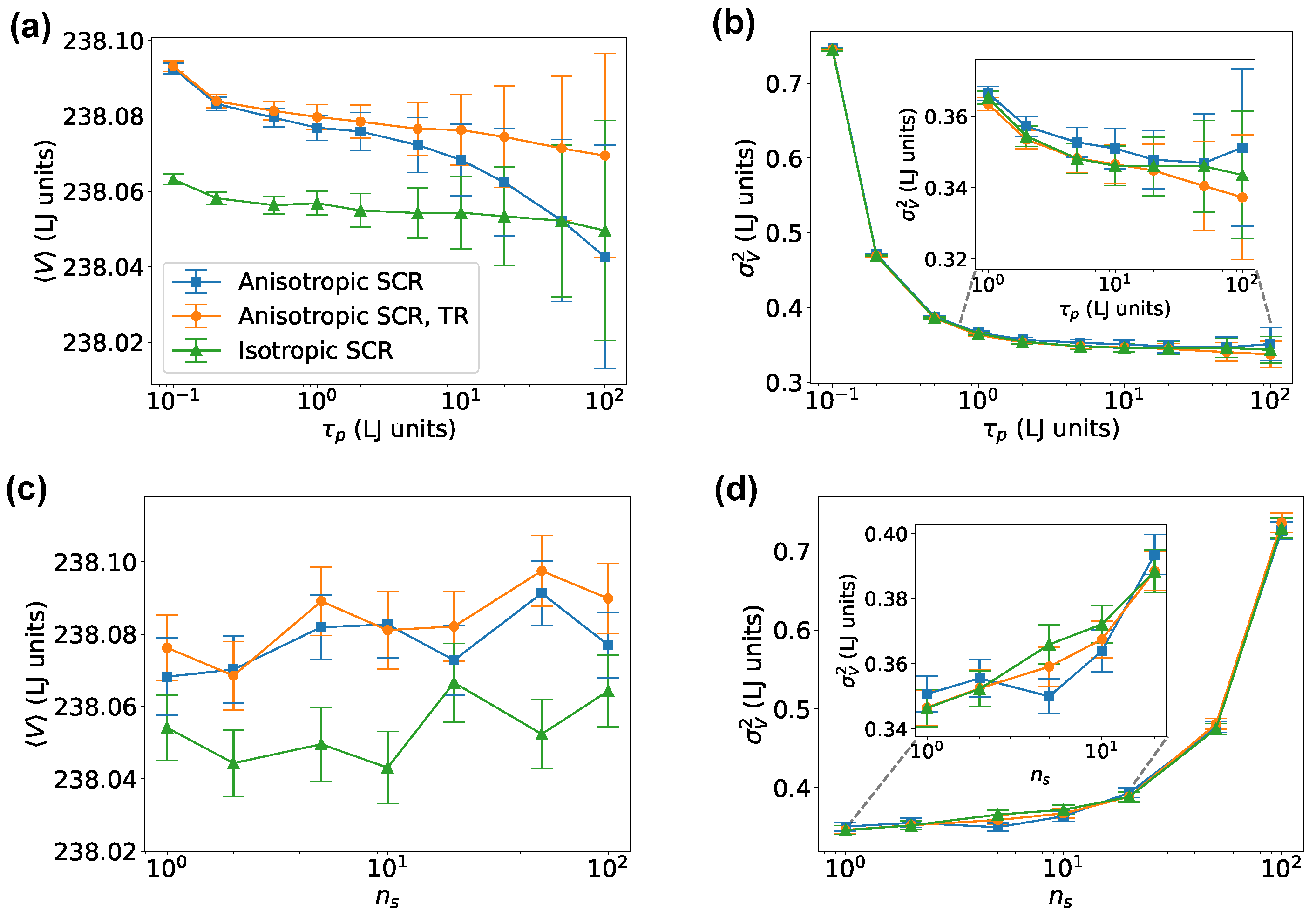
We first tested our algorithm on an fcc Lennard-Jones crystal. Results obtained using either the isotropic or the anisotropic implementations of the SCR and using both the simpler Euler integrator or the time-reversible one are reported in Figure 1, as functions of the barostat parameters ${\tau }_P$ and $n_s$. We underline that the SimpleMD implementation tested here is the only one supporting the time-reversible scheme discussed in Section 2.3.2. Figure 1a shows that systematic errors in the volume were negligible for ${\tau }_P⪆0.5$, whereas statistical errors, that were computed using block bootstrap and depended on the relaxation time of the volume, grew with ${\tau }_P$. The relative error in the average volume was extremely small in all cases. The small discrepancies between the volume distributions of the isotropic and anisotropic systems were a consequence of the finite size of the simulated system, as they appeared to shrink in the thermodynamic limit (see

Table 1. Differences between isotropic and anisotropic volume averages observed by simulating Lennard-Jones crystals of different sizes with SimpleMD. $N_{\mathrm{at}}$ is the number of atoms, ${\langle V\rangle }_{\mathrm{a}}$ and ${\langle V\rangle }_{\mathrm{i}}$ are the averages computed in the anisotropic and isotropic ensemble, respectively, and $\Delta \langle V\rangle ={\langle V\rangle }_{\mathrm{a}}-{\langle V\rangle }_{\mathrm{i}}$. Volumes were measured in Lennard-Jones units. Simulations were carried out with ${\tau }_p=1$, $n_s=1$ and with the same parameters described in Section 2.6.1.

${\mathit{N}}_{\mathbf{at}}$	${\langle \mathit{V}\rangle }_{\mathbf{i}}$	${\langle \mathit{V}\rangle }_{\mathbf{a}}$	$\mathbf{\Delta }\langle \mathit{V}\rangle$	$\mathbf{\Delta }\langle \mathit{V}\rangle /{\langle \mathit{V}\rangle }_{\mathbf{a}}$
256	238.057	238.077	0.020	0.0084%
500	464.962	464.979	0.017	0.0037%
1372	1275.873	1275.881	0.008	0.0006%

). A different scenario was seen in Figure 1b, where the systematic error on the volume variance was significantly dependent on the parameter ${\tau }_P$. We noted that a ${\tau }_P⪆10$ should have been used to make sure fluctuations were not significantly affected. Figure 1c,d reports the dependence of the volume average and variance on the multiple-time-stepping stride $n_s$. It can be seen that a too-aggressive choice of $n_s$ might significantly affect the estimated variance, and that, for this specific system, any choice $n_s⪅10$ produced correct results. All the results discussed here were obtained using the formulation where momenta were scaled and, in the anisotropic case, rotations were eliminated. However, the same simulations were also carried out without scaling momenta and without eliminating rotations, producing equivalent results.

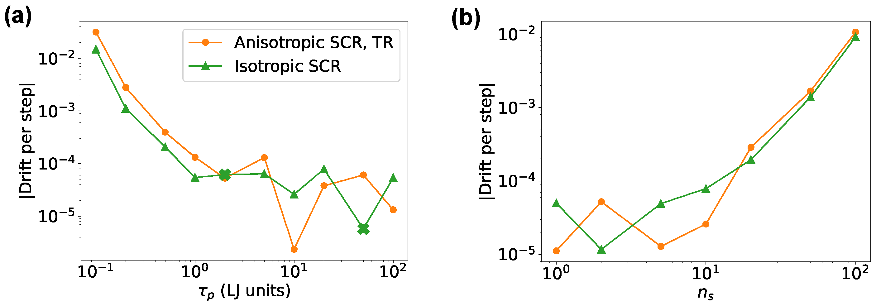
Figure 2 reports the effective energy drift that could be used as a measure of detailed balance violations. We noted that the drift became negligible at ${\tau }_P⪆2$. Beyond this value, its estimation was difficult due to the limited simulation length and the fact that the overall drift could not be distinguished from the effective energy fluctuations; thus, resulting in highly fluctuating or even negative estimates. The drift of the isotropic version followed the same trend as in Ref. [18]; in the anisotropic case, the drift was similar but slightly larger.

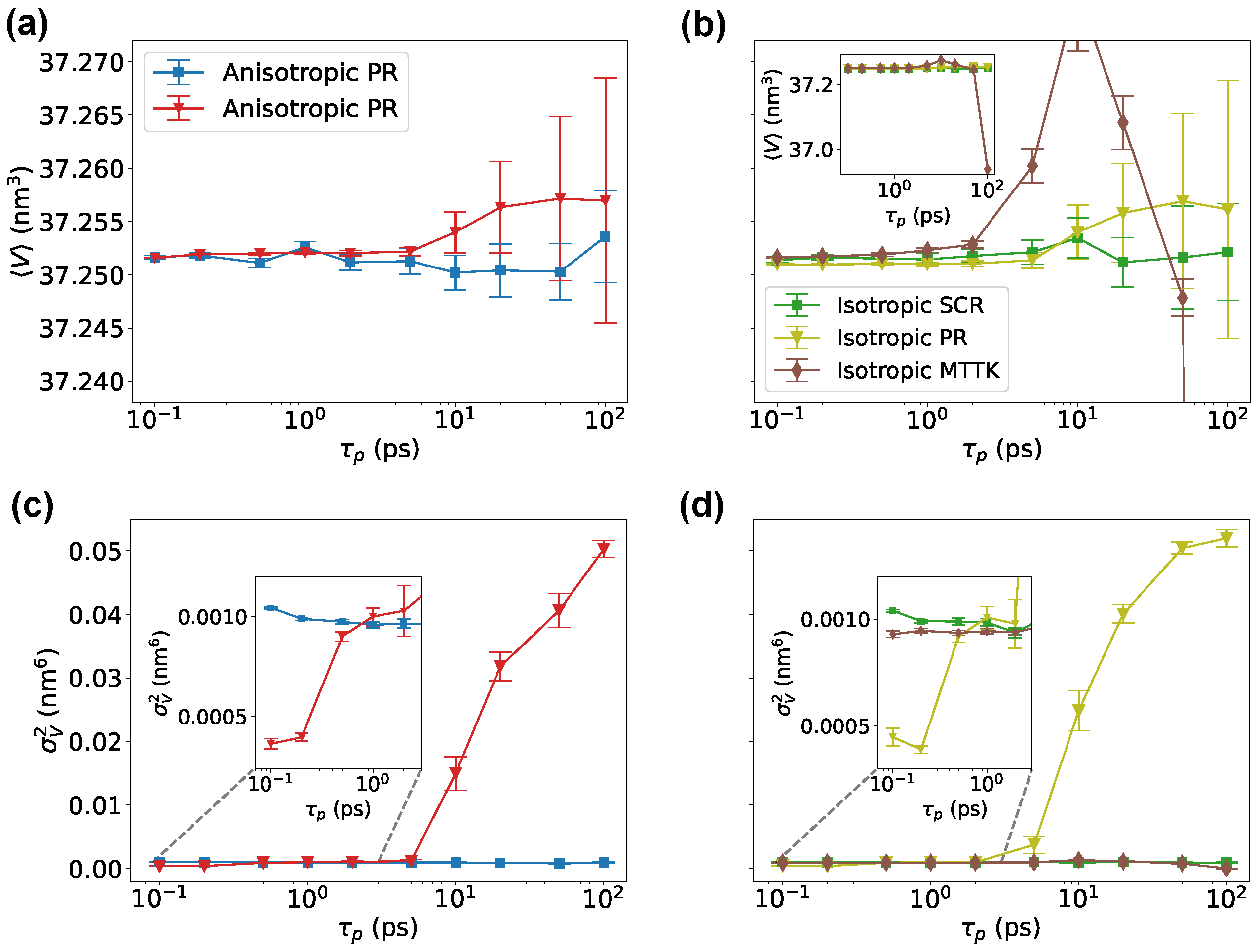
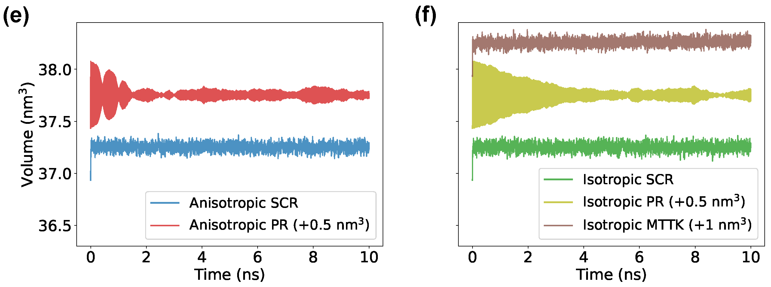
We then tested a Lennard-Jones system using the community code GROMACS. Here, we used physical units corresponding to the parametrization of Ar. Results were comparable to those obtained with SimpleMD, but allowed to directly compare SCR with the PR algorithm [3,4] and with the MTTK algorithm [8,9], as implemented in GROMACS (Figure 3). We noted that the MTTK algorithm was only implemented in its isotropic variant. Here, it can be seen that the averages and fluctuations for all methods were in agreement with each other when the ${\tau }_P$ parameter was properly chosen. It is important to remark here that there is not a direct equivalence in the choice of ${\tau }_P$ when using different methods. On the tested range of ${\tau }_P$, we observed that the anisotropic PR algorithm had problems in reproducing the correct volume fluctuations when ${\tau }_P⪅0.2$ ps. This problem might be related to details of the GROMACS implementation of this algorithm. For large values of ${\tau }_P$, instead, both the MTTK and the PR algorithms displayed significant problems in the estimated average or variance. These problems were due to the incorrect equilibration of the system (Figure 3e,f) and the persistent oscillations of the second-order algorithms.

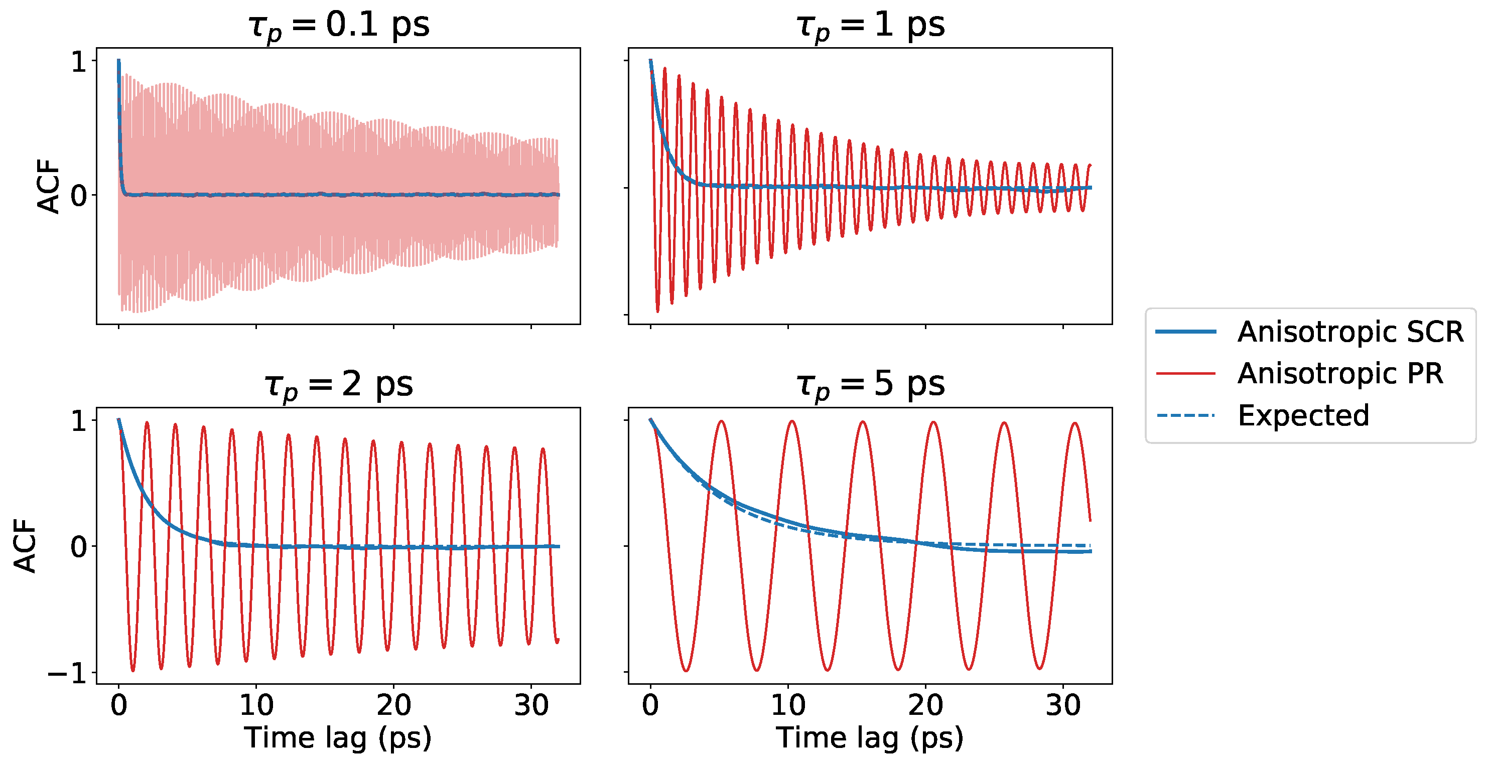
We reported in Figure 4 the auto-correlation functions of the volume using both SCR and PR algorithms for four different choices of ${\tau }_P$. This figure clearly shows the drawback of using a second-order algorithm, which led to fluctuations in the autocorrelation function that might be difficult to dampen. In particular, the envelope of the oscillations caused the damping time to increase when the relaxation time was lowered from 1 ps to 0.1 ps, suggesting the presence of an optimal value for the PR barostat that should be obtained by trial and error. The SCR algorithm, instead, resulted in an auto-correlation function that decayed with the time constant ${\tau }_p$, except for corrections depending on the error associated with the input isothermal compressibility (in this case, smaller than 6%).

The a priori knowledge on the volume autocorrelation time could be exploited to predict the statistical error of the volume average, $\mathrm{SE}\left[\langle V\rangle \right]$, by employing the well-known relation $\mathrm{SE}{\left[\langle V\rangle \right]}^2\simeq \frac{2{\tau }_P}{T}{\sigma }_V^2$, where T is the length of the simulation and the approximation holds for $T\gg {\tau }_p$ (see Figure 5a). The input parameter ${\tau }_p$ also carried information on the statistical errors associated with the estimate of the volume variance. Indeed, it was possible to show that the time series of the squared volume displacements from the average volume has a correlation time equal to $2{\tau }_p$ (a detailed discussion of this statement was reported in Ref. [25]). As a consequence, the statistical error associated with the volume variance could also be predicted accurately before performing any extensive analysis (see Figure 5b).

3.2. Crystal Ice I${}_h$

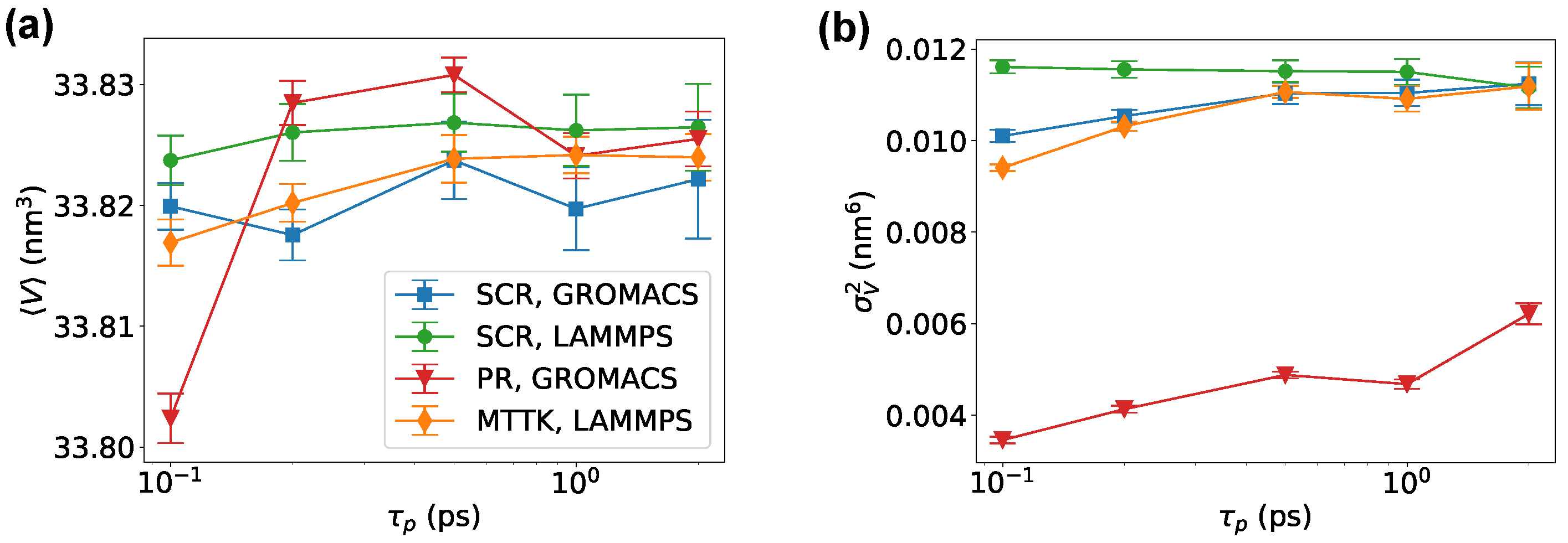
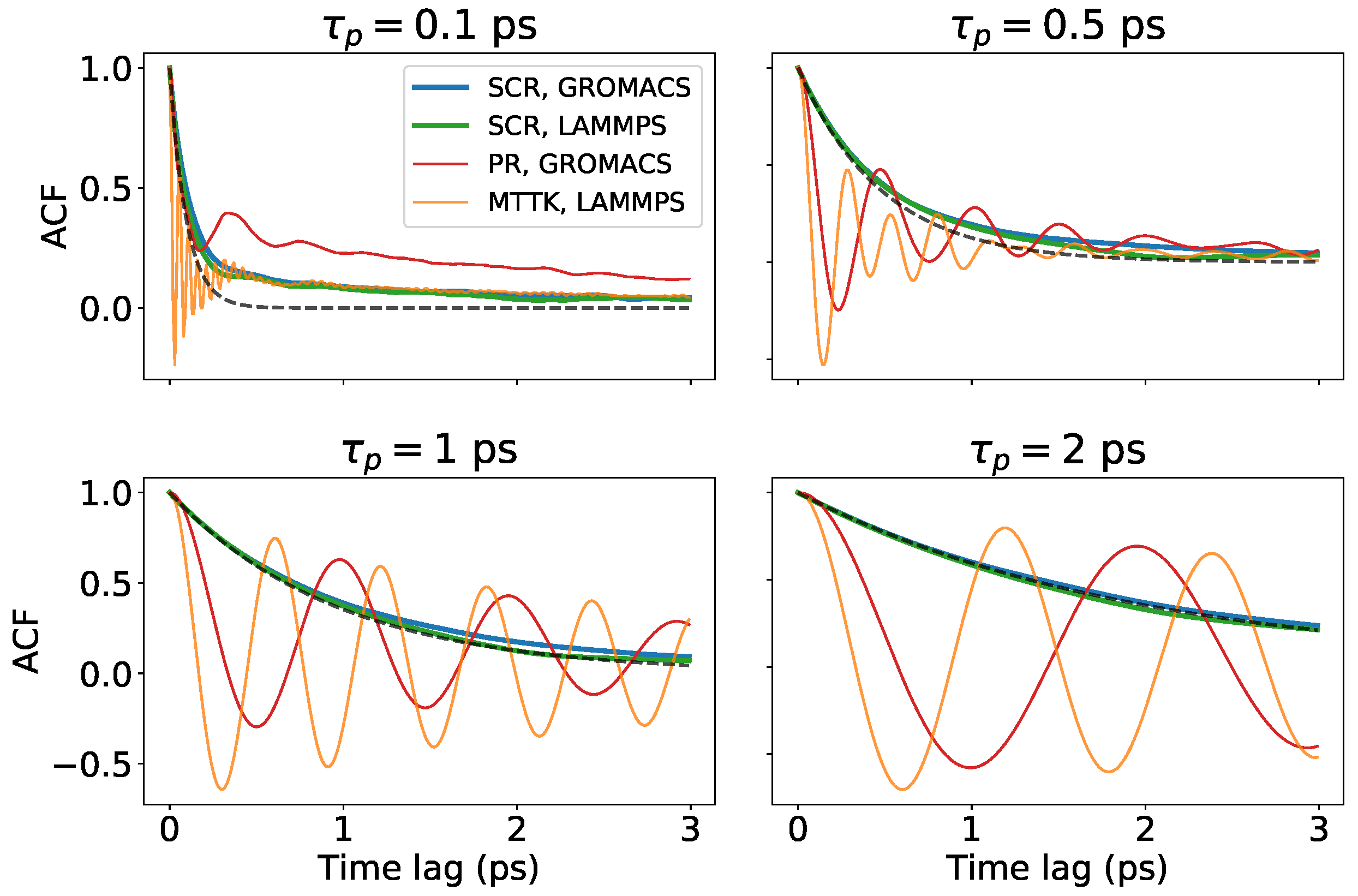
Next, we tested our algorithm on a crystalline ice I${}_h$ system. We simulated this system using both GROMACS and LAMMPS in order to test both implementations of the SCR scheme. In addition, we tested the PR implementation included in the GROMACS code and the MTTK implementation included in the LAMMPS code. The average and fluctuations of the volume are reported in Figure 6a,b. The two implementations of SCR reported similar results that also agreed with MTTK. The most striking difference was in the fluctuations reported by the PR implementation in GROMACS, that were systematically depending on ${\tau }_P$ in the tested range. We also reported the volume autocorrelation functions for different values of ${\tau }_P$ in Figure 7. Similarly to Figure 4, the difference between the second-order algorithms, where the volume oscillated, and the first-order SCR algorithm, where the volume relaxed to its average with an exponential decay, could be appreciated.

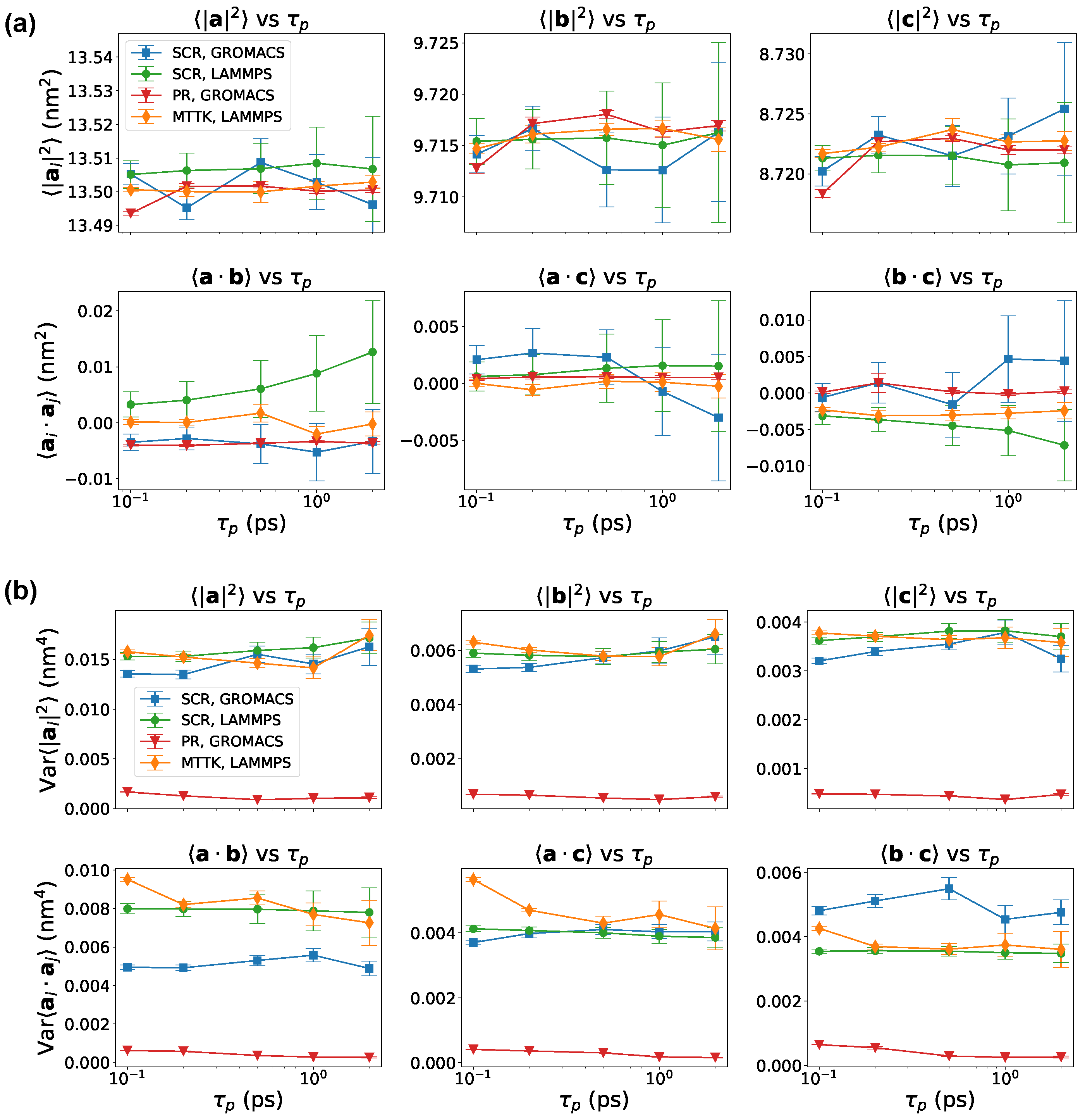
We also computed the average values and variances of the pairwise scalar products of the three lattice vectors. Results with all the tested schemes are reported in Figure 8. Results were consistent when ${\tau }_P$ was large enough. A notable exception was the PR implementation in GROMACS, that systematically underestimated fluctuations. We note again that the problem associated with the PR algorithm might be related to the details of its implementation in GROMACS, and not necessarily to the original PR algorithm.

3.3. Gypsum

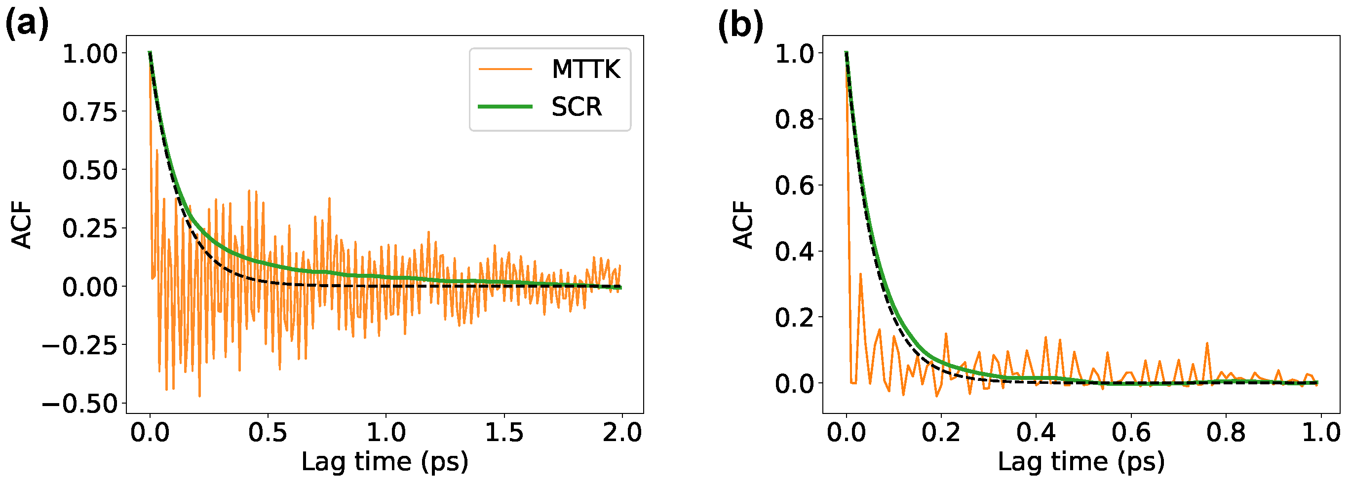
An additional test was performed on a gypsum crystal that was simulated with LAMMPS using both the anisotropic SCR and the MTTK barostat. Results obtained with the two barostats were consistent with each other and displayed comparable statistical errors (see

Table 2. Average and standard deviations of volume and potential energy for the simulated gypsum system, obtained both with anisotropic SCR and anisotropic MTTK barostats. Results were obtained setting ${\tau }_P=0.1$ ps.

	Anisotropic SCR	Anisotropic MTTK
$\langle V\rangle$ (nm${}^3$)	36.8682 ± 0.0008	36.8691 ± 0.0010
${\sigma }_V$ (nm${}^6$)	0.0624 ± 0.0003	0.0622 ± 0.0002
$\langle U\rangle$ (kJ/mol)	−789,541.4 ± 1.4	−789,542.3 ± 1.4
${\sigma }_U$ ((kJ/mol)${}^2$)	171.0 ± 0.7	170.5 ± 0.7

). The autocorrelation functions of the volume are reported in Figure 9, and were consistent with those reported for the Lennard-Jones (Figure 4) and ice (Figure 7) systems.

3.4. Gold Crystal

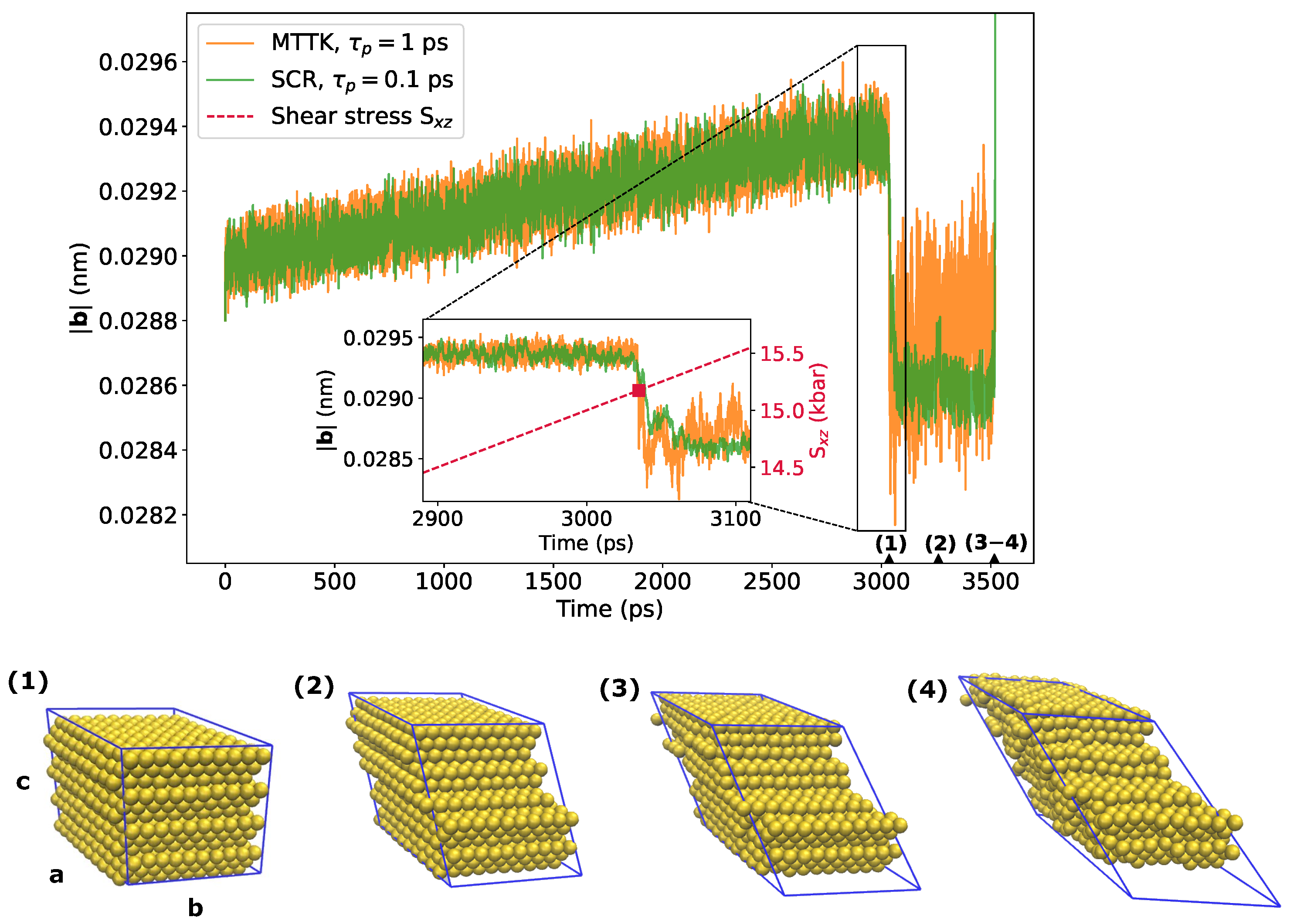
Finally, we tested the application of both SCR and the MTTK algorithm on the simulation of a gold crystal under a time-dependent $xz$ shear stress that was simulated with LAMMPS. The modulo of one of the lattice vectors was used to monitor the rupture of the structure. Its time series is reported in Figure 10, where it can be seen that the rupture happened at a shear stress of $S_{xz}\approx$ 15.1–15.3 kbar. This result was in agreement with the estimate obtained performing static calculations with the GULP software [42], a program more suited to lattice dynamics and geometry optimization calculations than to molecular dynamics. A visualization of the crystal breaking, which occurred through the slipping of the crystallographic planes (111), is also reported in Figure 10.

4. Discussion

In this work, we developed the fully anisotropic version of the stochastic cell rescaling (SCR) barostat that was introduced in Ref. [18]. The algorithm was then implemented in three different MD software packages and tested on a number of crystalline systems. When possible, results were compared with alternative algorithms already available in the tested codes. The isotropic and semi-isotropic versions introduced in Ref. [18] could be obtained as constrained cases of the equations of motion developed in this work. Additionally, this method could be shown to be equivalent to a Parrinello–Rahman barostat augmented with friction and noise terms, provided that the high-friction and zero-mass limit is taken.

The anisotropic SCR barostat is based on a first-order stochastic differential equation that describes the relaxation of the lattice vectors to their equilibrium values. The deterministic part of the equation resembles the anisotropic Berendsen barostat [17]. A crucial advantage of the anisotropic SCR barostat with respect to the Berendsen barostat is that, thanks to the noise term, the correct cell fluctuations are sampled. A single input parameter should be provided, ${\tau }_P$, that allows to enforce an approximate value for the relaxation time of the volume. For this approximation to hold, one should also provide an a priori estimation of the isothermal compressibility of the system ${\beta }_T$. In practice, only the value of $\frac{{\beta }_T}{{\tau }_P}$ is used in the resulting equations of motion. Hence, an incorrect estimate of the isothermal compressibility would result in an observed relaxation time different from ${\tau }_P$. This issue is common with the Berendsen barostat [17]. Nevertheless, the analyses carried out in this work showed that the method is robust against variations of ${\tau }_p$ within 2–3 orders of magnitude, suggesting no significant effects on the sampled $N\mathbf{S}T$ distribution if the input ${\beta }_T$ is estimated with the correct order of magnitude.

Two integrators were developed and tested. One of them is simpler and could be straightforwardly integrated in existing MD codes. The other one is more complicated as it requires propagating position and velocities simultaneously to lattice vectors, and was only implemented in the SimpleMD code. The second integrator has the advantage of being time-reversible and, thus, allowing detailed balance violations to be quantified.

In our algorithm, velocities could be optionally scaled when the lattice vectors were modified. We propose to use a scaling matrix for velocities that is the inverse transpose of the matrix used to scale positions. This is different from the standard procedure used in Refs. [8,9,16], where it can be shown that both positions and velocities were rescaled with exponential matrices in the limit of small $\Delta t$, and these matrices were the inverse of each other. To the best of our knowledge, this idea is new, and allows rotations to be handled consistently on position and velocities, which is expected to be more effective when simulating systems with holonomic constraints. This advantage was present when global rotations were removed by keeping the cell matrix triangular, since, in this case, the transformation matrix was not symmetric. It is, instead, irrelevant when implementing the MTTK algorithm constraining the cell momentum matrix to be symmetric [8], since, in this case, the transformation matrix was also symmetric. Indeed, this approach has been argued to be more effective in simulating systems with constraints [1]. It is also irrelevant in the isotropic or semi-isotropic cases implemented in Ref. [18], since, in those cases, the transformation matrix was diagonal.

Similarly to the isotropic version, it was possible to avoid the scaling of velocities resulting in a different definition of the internal pressure and a slightly simplified integrator. This possibility was tested here for the Lennard-Jones system and did not offer any specific advantage. It was, instead, expected to be less effective in more general settings, such as using constraints; thus, we did not test it further. An alternative option would be to use the molecular virial and scale only the molecular positions and, optionally, velocities. In this case, intramolecular distances and velocities would not be affected by the scaling procedure and one could, thus, use the formulation where velocities are not scaled also in the presence of intramolecular constraints.

The choice of ${\tau }_P$ should be determined with care. A too low of a value could result in systematic errors due to difficulties in the integration of the equation of motions. This type of error could be detected by comparing results for different values of ${\tau }_P$ or, when using the time-reversible integrator, by monitoring the effective energy drift, which reports on the detailed balance violation. Although there is no unique prescription about which drift magnitude could be acceptable, one might, for instance, make sure that the drift is similar to the one obtained from a constant volume simulation of the same system. This result would suggest that the integration errors associated with the barostat are not exceeding those associated with the solution of the Hamilton equations of motion for the simulated particles. A too large value of ${\tau }_P$, instead, would result in a slow volume relaxation. If an approximate estimate of the isothermal compressibility of the system ${\beta }_T$ was allowed, it would be easy to choose a ${\tau }_P$ small enough to allow fluctuations of the cell volume to be properly sampled on the desired time scale.

An important advantage of the anisotropic SCR, when compared with standard barostats relying on second-order differential equations, is that the relaxation of the volume was more easily predictable and would not exhibit oscillations. This caused the introduced algorithm to be more robust in equilibration procedures. The relaxation of the individual components of the cell matrix seemed more difficult to predict. A possible extension would be to use a tensor compressibility so as to allow individual relaxation times to be controlled. The corresponding equations were developed in Ref. [25], but have not yet been tested.

Additional material, including the implementations of the anisotropic SCR barostat in SimpleMD, GROMACS, and LAMMPS, and a Python notebook that can be used to reproduce all the figures of this article, can be found in the GitHub repository https://github.com/bussilab/crescale (accessed on 5 December 2021) and in linked repositories.

References

- Tuckerman, M. Statistical Mechanics: Theory and Molecular Simulation; Oxford University Press: Oxford, UK, 2010. [Google Scholar]
- Andersen, H.C. Molecular dynamics simulations at constant pressure and/or temperature. J. Chem. Phys. 1980, 72, 2384–2393. [Google Scholar] [CrossRef] [Green Version]
- Parrinello, M.; Rahman, A. Crystal structure and pair potentials: A molecular-dynamics study. Phys. Rev. Lett. 1980, 45, 1196–1199. [Google Scholar] [CrossRef]
- Parrinello, M.; Rahman, A. Polymorphic transitions in single crystals: A new molecular dynamics method. J. Appl. Phys. 1981, 52, 7182–7190. [Google Scholar] [CrossRef]
- Fay, P.J.; Ray, J.R. Monte Carlo simulations in the isoenthalpic-isotension-isobaric ensemble. Phys. Rev. A 1992, 46, 4645–4649. [Google Scholar] [CrossRef] [PubMed]
- Vandenhaute, S.; Rogge, S.M.; Van Speybroeck, V. Large-Scale Molecular Dynamics Simulations Reveal New Insights Into the Phase Transition Mechanisms in MIL-53 (Al). Front. Chem. 2021, 9, 699. [Google Scholar] [CrossRef] [PubMed]
- Wentzcovitch, R.M. Invariant molecular-dynamics approach to structural phase transitions. Phys. Rev. B 1991, 44, 2358. [Google Scholar] [CrossRef] [PubMed]
- Martyna, G.J.; Tobias, D.J.; Klein, M.L. Constant pressure molecular dynamics algorithms. J. Chem. Phys. 1994, 101, 4177–4189. [Google Scholar] [CrossRef]
- Martyna, G.J.; Tuckerman, M.E.; Tobias, D.J.; Klein, M.L. Explicit reversible integrators for extended systems dynamics. Mol. Phys. 1996, 87, 1117–1157. [Google Scholar] [CrossRef]
- Souza, I.; Martins, J. Metric tensor as the dynamical variable for variable-cell-shape molecular dynamics. Phys. Rev. B 1997, 55, 8733. [Google Scholar] [CrossRef] [Green Version]
- Yu, T.Q.; Alejandre, J.; López-Rendón, R.; Martyna, G.J.; Tuckerman, M.E. Measure-preserving integrators for molecular dynamics in the isothermal–isobaric ensemble derived from the Liouville operator. Chem. Phys. 2010, 370, 294–305. [Google Scholar] [CrossRef]
- Raiteri, P.; Gale, J.D.; Bussi, G. Reactive force field simulation of proton diffusion in BaZrO3 using an empirical valence bond approach. J. Phys. Condens. Matter 2011, 23, 334213. [Google Scholar] [CrossRef] [PubMed] [Green Version]
- Quigley, D.; Probert, M.I.J. Langevin dynamics in constant pressure extended systems. J. Chem. Phys. 2004, 120, 11432–11441. [Google Scholar] [CrossRef] [PubMed]
- Gao, X.; Fang, J.; Wang, H. Sampling the isothermal-isobaric ensemble by Langevin dynamics. J. Chem. Phys. 2016, 144, 124113. [Google Scholar] [CrossRef] [PubMed] [Green Version]
- Cajahuaringa, S.; Antonelli, A. Stochastic sampling of the isothermal-isobaric ensemble: Phase diagram of crystalline solids from molecular dynamics simulation. J. Chem. Phys. 2018, 149, 064114. [Google Scholar] [CrossRef] [Green Version]
- Shinoda, W.; Shiga, M.; Mikami, M. Rapid estimation of elastic constants by molecular dynamics simulation under constant stress. Phys. Rev. B 2004, 69, 134103. [Google Scholar] [CrossRef]
- Berendsen, H.J.C.; Postma, J.P.M.; van Gunsteren, W.F.; Di Nola, A.; Haak, J.R. Molecular dynamics with coupling to an external bath. J. Chem. Phys. 1984, 81, 3684–3690. [Google Scholar] [CrossRef] [Green Version]
- Bernetti, M.; Bussi, G. Pressure control using stochastic cell rescaling. J. Chem. Phys. 2020, 153, 114107. [Google Scholar] [CrossRef]
- Abraham, M.J.; Murtola, T.; Schulz, R.; Páll, S.; Smith, J.C.; Hess, B.; Lindahl, E. GROMACS: High performance molecular simulations through multi-level parallelism from laptops to supercomputers. SoftwareX 2015, 1–2, 19–25. [Google Scholar] [CrossRef] [Green Version]
- Thompson, A.P.; Aktulga, H.M.; Berger, R.; Bolintineanu, D.S.; Brown, W.M.; Crozier, P.S.; Veld, P.J.i.; Kohlmeyer, A.; Moore, S.G.; Nguyen, T.D.; et al. LAMMPS—A flexible simulation tool for particle-based materials modeling at the atomic, meso, and continuum scales. Comput. Phys. Commun. 2022, 271, 108171. [Google Scholar] [CrossRef]
- Zhang, Y.; Feller, S.E.; Brooks, B.R.; Pastor, R.W. Computer simulation of liquid/liquid interfaces. I. Theory and application to octane/water. J. Chem. Phys. 1995, 103, 10252–10266. [Google Scholar] [CrossRef]
- Gardiner, C.W. Handbook of Stochastic Methods; Springer: Berlin, Germany, 2009. [Google Scholar]
- Bussi, G.; Zykova-Timan, T.; Parrinello, M. Isothermal-isobaric molecular dynamics using stochastic velocity rescaling. J. Chem. Phys. 2009, 130, 074101. [Google Scholar] [CrossRef] [PubMed] [Green Version]
- Bussi, G.; Donadio, D.; Parrinello, M. Canonical sampling through velocity rescaling. J. Chem. Phys. 2007, 126, 014101. [Google Scholar] [CrossRef] [PubMed] [Green Version]
- Del Tatto, V. A Fully Anisotropic Formulation of Stochastic Cell Rescaling. arXiv 2021, arXiv:2111.06402. [Google Scholar]
- Grønbech-Jensen, N.; Farago, O. Constant pressure and temperature discrete-time Langevin molecular dynamics. J. Chem. Phys. 2014, 141, 194108. [Google Scholar] [CrossRef] [PubMed] [Green Version]
- Jung, J.; Kobayashi, C.; Sugita, Y. Optimal temperature evaluation in molecular dynamics simulations with a large time step. J. Chem. Theory Comput. 2018, 15, 84–94. [Google Scholar] [CrossRef]
- Tuckerman, M.E.; Martyna, G.J.; Berne, B.J. Molecular dynamics algorithm for condensed systems with multiple time scales. J. Chem. Phys. 1990, 93, 1287–1291. [Google Scholar] [CrossRef]
- Arioli, M.; Codenotti, B.; Fassino, C. The Padé method for computing the matrix exponential. Linear Algebra Its Appl. 1996, 240, 111–130. [Google Scholar] [CrossRef] [Green Version]
- Bussi, G.; Parrinello, M. Accurate sampling using Langevin dynamics. Phys. Rev. E 2007, 75, 056707. [Google Scholar] [CrossRef] [Green Version]
- Sivak, D.A.; Chodera, J.D.; Crooks, G.E. Using nonequilibrium fluctuation theorems to understand and correct errors in equilibrium and nonequilibrium simulations of discrete Langevin dynamics. Phys. Rev. X 2013, 3, 011007. [Google Scholar] [CrossRef] [Green Version]
- Scemama, A.; Lelièvre, T.; Stoltz, G.; Cancès, E.; Caffarel, M. An efficient sampling algorithm for variational Monte Carlo. J. Chem. Phys. 2006, 125, 114105. [Google Scholar] [CrossRef] [Green Version]
- Manousiouthakis, V.I.; Deem, M.W. Strict detailed balance is unnecessary in Monte Carlo simulation. J. Chem. Phys. 1999, 110, 2753–2756. [Google Scholar] [CrossRef] [Green Version]
- Fass, J.; Sivak, D.A.; Crooks, G.E.; Beauchamp, K.A.; Leimkuhler, B.; Chodera, J.D. Quantifying configuration-sampling error in Langevin simulations of complex molecular systems. Entropy 2018, 20, 318. [Google Scholar] [CrossRef] [PubMed] [Green Version]
- Schmid, N.; Eichenberger, A.P.; Choutko, A.; Riniker, S.; Winger, M.; Mark, A.E.; van Gunsteren, W.F. Definition and testing of the GROMOS force-field versions 54A7 and 54B7. Eur. Biophys. J. 2011, 40, 843–856. [Google Scholar] [CrossRef] [PubMed]
- Abascal, J.; Sanz, E.; García Fernández, R.; Vega, C. A potential model for the study of ices and amorphous water: TIP4P/Ice. J. Chem. Phys. 2005, 122, 234511. [Google Scholar] [CrossRef] [Green Version]
- Hess, B.; Bekker, H.; Berendsen, H.J.C.; Fraaije, J.G.E.M. LINCS: A linear constraint solver for molecular simulations. J. Comput. Chem. 1997, 18, 1463–1472. [Google Scholar] [CrossRef]
- Darden, T.; York, D.; Pedersen, L. Particle mesh Ewald: An N log (N) method for Ewald sums in large systems. J. Chem. Phys. 1993, 98, 10089–10092. [Google Scholar] [CrossRef] [Green Version]
- Byrne, E.H.; Raiteri, P.; Gale, J.D. Computational Insight into Calcium–Sulfate Ion Pair Formation. J. Phys. Chem. C 2017, 121, 25956–25966. [Google Scholar] [CrossRef]
- Söngen, H.; Silvestri, A.; Roshni, T.; Klassen, S.; Bechstein, R.; Raiteri, P.; Gale, J.D.; Kühnle, A. Does the Structural Water within Gypsum Remain Crystalline at the Aqueous Interface? J. Phys. Chem. C 2021, 125, 21670–21677. [Google Scholar] [CrossRef]
- Ryu, S.; Weinberger, C.R.; Baskes, M.I.; Cai, W. Improved modified embedded-atom method potentials for gold and silicon. Model. Simul. Mater. Sci. Eng. 2009, 17, 075008. [Google Scholar] [CrossRef]
- Gale, J.D. GULP: A computer program for the symmetry-adapted simulation of solids. J. Chem. Soc. Faraday Trans. 1997, 93, 629–637. [Google Scholar] [CrossRef]
Figure 1.
Volume average and fluctuations for an fcc Lennard-Jones crystal simulated with SimpleMD. Average (a) and variance (b) of the cell volume as functions of the barostat relaxation time , setting . Average (c) and variance (d) of the cell volume as functions of the multiple-time-stepping stride , setting . Insets in panels (b,d) are used to show the large and low regimes, respectively. TR denotes the time-reversible integrator (see Section 2.3.2).
Figure 2.
Effective energy drift for an fcc Lennard-Jones crystal simulated with SimpleMD. Results for both the isotropic and anisotropic versions are reported as a function of the barostat relaxation time in panel (a) and as a function of the barostat stride in panel (b). TR denotes the time-reversible integrator (see Section 2.3.2). Absolute value is reported in the figure. The drift was positive for all the points, except for those marked with a cross, for which the drift was negative.
Figure 3.
Volume average and fluctuations for a cubic Lennard-Jones crystal simulated with GROMACS. Panels (a,b) show the average volume using SCR, PR, and MTTK algorithms, in their anisotropic and isotropic variants, as indicated. Variance of the volume is reported in panels (c,d). Examples of non-converging volume trajectories for the PR barostat are shown in panels (e,f), for simulations carried out with ps.
Figure 4.
Autocorrelation functions of the volume for the hexagonal close-packed Lennard-Jones crystal simulated using GROMACS. Results were obtained using both stochastic cell rescaling and PR algorithms, in their anisotropic variants, with four different choices of the barostat parameter . The dashed lines report exponentially decaying functions with time constants , where is the isothermal compressibility computed from the simulations and is the input one.
Figure 5.
Relative errors on the estimates of volume average—panel (a)—and volume variance—panel (b)—from the simulations of the Lennard-Jones crystal using GROMACS. Different values of were scanned between 0.1 ps and 5 ps.
Figure 6.
Results for crystal ice I simulated with GROMACS and LAMMPS. Average (a) and variance (b) of the volume as functions of , for different barostats and codes as indicated.
Figure 7.
Results for crystal ice I simulated with GROMACS and LAMMPS. Autocorrelation functions of the volume for different algorithms and codes, obtained with different choices of , as indicated. The dashed lines represent the expected decaying functions .
Figure 8.
Results for crystal ice I simulated with GROMACS and LAMMPS. Averages—panels (a)—and variances—panels (b)—of pairwise scalar products among the lattice vectors, reported as a function of , for different barostats and codes as indicated.
Figure 9.
Results from the simulations of the gypsum with LAMMPS, obtained using both stochastic cell rescaling and MTTK algorithms, in their anisotropic variants. Panel (a): Autocorrelation functions of the volume. The dashed line reports an exponentially decaying function with time constant . Panel (b): Autocorrelation function for the series of squared volume displacements from the volume average. The dashed line corresponds to an exponential decay with time constant .
Figure 10.
Results from the simulations of the gold crystal systems in LAMMPS, employing the MTTK and SCR anisotropic barostats in presence of a linearly increasing shear stress. The plot shows the trajectory for the modulus of the cell vector , which is a good variable to describe the crystal breaking. Selected structures are shown with the corresponding sampling times along the horizontal axis.