
Multimode Tree-Coding of Speech with Pre-/Post-Weighting †


1
MediaTek Inc., No. 1, Dusing 1st Road, Hsinchu Science Park, Hsinchu City 30078, Taiwan
2
Qualcomm, Inc., 5775 Morehouse Drive, San Diego, CA 92121, USA
3
Department of Electrical and Computer Engineering, University of California, Santa Barbara, CA 93106, USA
*
Author to whom correspondence should be addressed.
†
This paper is an extended version of our paper published in Y.-Y. Li and J. D. Gibson, Multimode Tree Coding of Speech with Backward Pitch Prediction and Perceptual Pre- and Post-weighting, 46th Annual Asilomar Conference on Signals, Systems, and Computers, Pacific Grove, CA, USA, 4–7 November 2012.
‡
These authors contributed equally to this work. The work of Ying-Yi Li and Pravin Ramadas was accomplished while they were affiliated with the University of California, Santa Barbara.
Appl. Sci. 2022, 12(4), 2026; https://doi.org/10.3390/app12042026
Submission received: 15 December 2021
/
Revised: 31 January 2022
/
Accepted: 10 February 2022
/
Published: 15 February 2022
(This article belongs to the Section Electrical, Electronics and Communications Engineering)
Abstract
:Featured Application
Applications for the speech codecs presented in this paper are Voice over Internet Protocol, digital cellular communications, and video telephony.
Abstract
As speech-coding standards have improved over the years, so complexity has increased, and less emphasis been placed on low encoding/decoding delay. We present a low-complexity, low-delay speech codec based on tree-coding with sample-by-sample adaptive long- and short-code generators that incorporates pre- and post-filtering for perceptual weighting and multimode speech classification with comfort noise generation (CNG). The pre-/post-weighting filters adapt based on the code generator parameters available at both the encoder and decoder rather than the usual method that uses the input speech. The coding of the multiple speech modes and comfort noise generation is accomplished using the code generator adaptation algorithms, again, rather than using the input speech. Codec complexity comparisons are presented and operational rate distortion curves for several standardized speech codecs and the new codec are given. Finally, codec performance is shown in relation to theoretical rate distortion bounds.
1. Introduction
Speech-coding has a history of more than 50 years, but the current research directions involving linear prediction can be traced back to the mid to late 1960s [1,2]. As standards were developed for narrowband speech (300 to 3400 Hz bandwidth), first in digital telephony over the circuit-switched telephone network, followed by video telephony and digital cellular applications, bit rates were pushed lower and more complexity and latency in the encoding/decoding processes were admitted. More recent forays into speech-coding standards incorporate wideband speech for inputs in the 50 Hz to 7 kHz band and audio bandwidths of 20 Hz to 20 kHz and additional functionalities involving better input and output processing. Coupled with computational advances driven by Moore’s Law, these codecs are extraordinarily complex, and latencies can grow well above 20 msec. High complexity is an obvious challenge in many applications, particularly with respect to battery power for mobile devices, and increased latency can impact conversational voice quality, and perhaps more subtly, cellular capacity.
With these ideas in mind, we have conducted research on speech codecs that have greatly reduced complexity and latency, while attempting to strike a performance balance between coded speech quality and required bitrate. The codec structure presented in this paper uses a type of analysis-by-synthesis coding called tree-coding, which employs a codec that has the form of a tree. The tree depth is much shorter than the usual block length used for the code searching in Code-Excited Linear Prediction (CELP). See Section 2 and references cited there. To reduce complexity, the perceptual weighting filter is moved out of the analysis-by-synthesis loop and incorporated as pre-weighting and post-weighting filters. Additionally, the short-term and long-term predictors as well as the codec gain are adapted on a sample-by-sample basis using what are called backward adaptive algorithms, which along with the shallow search depth, leads to lower delay than for codecs such as AMR and EVS. Furthermore, the input speech is classified into modes, which are coded separately. Since this coder uses multiple modes, perceptual pre- and post-weighting, tree searching, and a pitch predictor, it is denoted as the Multimode Tree Coder with Pre- and Post-Weighting and Pitch prediction (MMT-WP) coder.
The particular codec described and analyzed here, MMT-WP, was first presented in [3] where its performance was compared with a Multimode Tree Coder (MMT) based on G.727 and a squared error fidelity criterion and a MMT with pre-weighting and post-weighting to add perceptual shaping to the fidelity criterion, designated here as MMT-W, the multimode tree coder with pre- and post-weighting but no pitch prediction. It is shown in that paper that the MMT-WP outperforms the MMT codec without perceptual weighting and without pitch prediction in terms of PESQ-MOS [4]. These results are not included here, and substantial new discussion and performance results are presented as discussed at the end of this Introduction. The overall structure of the MMT-WP codec is presented in Section 3, which briefly introduces the several components.
The G.727 waveform-following codec that uses backward adaptive short-term prediction and quantization is discussed in Section 4. The details of the predictor adaptation are included in Section 4.1 and the quantizer adaptation is covered in Section 4.2. These descriptions are included since parameters from G.727 are used in the voice activity detection and mode decisions and the reasons for zeros in the predictor are developed later as well. The G.727 performance is improved by the addition of a long-term pitch predictor, which is described in Section 5. The G.727 codec with the long-term pitch predictor forms the basis for what is called the Code Generator in Tree-Coding. Section 6 very briefly presents the basic building blocks of a tree coder, including the Code Generator, the Code Tree, the Tree Search, Algorithm, and the Perceptual Distortion Measure, which is usually inside the analysis-by-synthesis loop.
The justification and analysis of moving the perceptual distortion measure outside the analysis-by-synthesis loop are given in Section 7. Section 8 develops the novel voice activity detection and mode detection procedures using the G.727 codec parameters and shows the classification results for the sentences used for the initial studies. Zeros were included in the original G.727 to maintain prediction performance when the all-pole predictor order was reduced for stability reasons. Zeros are part of the short-term predictor in the MMT-WP codec for the different reasons briefly discussed in Section 9. Performance analyses of the MMT-WP codec start in Section 10, where the different Comfort Noise Generation (CNG) methods and the corresponding bit rates are given and then the performance with the different CNG coding methods is presented. One of the goals of the current research is to reduce the codec complexity and Section 11 analyzes the complexity of the MMT-WP codec per component and per sentence. Section 13 presents comparisons of the operational rate distortion functions of the MMT-WP codec and the AMR-NB, G.727, and G.728 codecs for the utterances studied. Comparisons of the operational rate distortion functions with the rate distortion bounds are given in Section 14 to see how far away these codecs are from the optimum performance theoretically attainable for the source models developed using the approach of Gibson and Hu [5].
In comparison to the conference paper in [3], this paper has an extensive discussion of speech-coding background and current work in Section 2, a clearer development of the voice activity detection and mode decisions in Section 8, a justification of using zeros in the predictor in Section 9, a new section, Section 12, describing current voice codecs and comparisons in terms of complexity, latency, performance, and functionality in relation to the goals of the current research, an expansion of the performance comparisons to other standardized codecs in terms of operational rate distortion functions in Section 13, and the inclusion of new results on the proposed codec compared to theoretically calculated rate distortion bounds in Section 14.
Finally, some suggestions for extending the MMT-WP codec for wideband speech inputs and ideas for other future work are given in Section 15 along with conclusions.
The following section on Speech-Coding Background, Section 2, places this research in the context of the various speech-coding standards and some on-going speech-coding research.
2. Speech-Coding Background
In the past few decades, speech-coding research and development has been dominated by efforts to standardize speech codecs for different applications [6,7]. Initial applications were for narrowband (NB) or telephone bandwidth speech, which refers to speech occupying the band 300 Hz to 3400 Hz, and were for wireline telephony in the circuit-switched digital telephone network and then the emphasis turned to digital cellular communications. Starting with G.729, a NB speech codec operating at 8 kbps [8], the primary approach to speech-coding since has been analysis-by-synthesis (AbS) coding using a codebook excitation, called Code-Excited Linear Prediction (CELP). This codec produced unheard of performance at that design rate. Interest then turned to developing codecs for wideband (WB) speech, which occupies the band 50 Hz to 7 kHz, to allow sharper sounding and more intelligible speech than possible with NB speech. This effort led to the establishment of the Adaptive Multirate (AMR) codec that has both narrowband and wideband capabilities and a range of transmitted bit rates [9,10].
More recently, the speech-coding standards activity turned to not only improving the quality of the coded speech at the desired bit rates for both NB and WB speech, but also to incorporating the capability of coding music in wider bands and detecting and compensating for noisy environments. This work led to the standardization of the Enhanced Voice Services (EVS) codec with truly remarkable performance [11]. Despite the availability of the new EVS codec, AMR continues to be the most installed and used codec in the World. AMR-WB is also the currently preferred codec for First Responder voice communications in the U. S. over LTE by First Net because of its widely installed base and the years of reliable performance, which is needed for first responder voice communications.
Specific details of the performance, complexity, and latency for many standardized codecs are available in Gibson [6]. An overview of the field of speech-coding standards and speech-coding research, including the relationship between speech and audio coding and future challenges, is presented in [7], wherein extensive key references to the literature are included. These publications point out the leading role played by the AMR-WB and AMR-NB speech codecs in VoIP and digital cellular communications throughout the World. The discussion of the EVS codec points out that this new codec is designed for multi-functionality by providing the ability to code narrowband, wideband, and super wideband speech as well as audio. Both increased front end and output signal processing addresses issues such as background noise in the input and smooth switching between bandwidths and coding modes at the output. This greatly increased functionality comes with a corresponding tremendous increase in complexity and an increase in total latency.
Not included in the references [6,7] is a discussion of the application of Deep Learning to speech-coding, which is receiving some research attention. The success of Deep Learning for speech recognition has motivated research into the use of deep learning for speech-coding. Speech-coding is not quite as good a fit for deep neural networks as for speech recognition, for example, since latencies greater than a few tenths of a second can preclude person-to-person voice communications and since the encoding and decoding must be accomplished in real time on mobile handsets (for the primary application). Furthermore, researchers in neural networks and learning also desire, as is the vogue in deep learning applications today, end-to-end speech-coding, meaning speech-coding without any, or at least minimal, domain knowledge.
These research goals are challenging since current speech codecs operate in real time with under a tenth of a second for encoding cascaded with decoding, are implementable on moderate complexity mobile devices, work well for multiple languages, and achieve excellent quality and intelligibility, allowing the listener to not only understand what is being said but also to identify the speaker. There are limits to speech codecs today, but those limits tend to be on the naturalness and intelligibility achievable at lower bit rates such as 4 kilobits/sec and below, and on increased complexity and ever-increasing latency.
However, the lure of end-to-end speech-coding without the expertise of a domain expert and trainable in hours or days rather than requiring years for codec design is sufficiently strong that several researchers/research groups have been motivated to approach the problem [12,13,14,15,16]. The study by Kankanahalli [12] on using deep neural networks (DNNs) to design an “end-to-end” speech codec captures the challenges faced when designing a speech codec with minimal domain knowledge. First, the term end-to-end is usually intended to mean that the raw signal is input and the DNN does the rest–no domain knowledge required. For speech-coding, all the papers choose a window, a window size, and an overlap of the adjacent windows to package the raw data before passing it on to the DNN. These choices are significant and domain knowledge and experimentation should be used in their selection. The work in [12] used a 32 msec (512 samples at 16,000 samples/s) Hann window with 2 msec overlap (32 samples) for adjacent windows. A greater overlap of the windows would likely produce better results. The speech codec in [12] employed an additional much more domain knowledge assumption since it used mel frequency cepstral coefficients (MFCCs) within a sum of squared error perceptual distortion measure.
In the training process for the DNN-based codec, a separate network is trained for each bitrate targeted and each network required about 20 h of training on a GeForce GTX 1080 Ti GPU. Encoding and decoding time is nearly equally split and the average time it takes for encoding and decoding of a 30 msec window using an Intel i7-4970K CPU (3.8 GHz) and the GeForce GTX 1080 Ti GPU is about 26 msec. The conclusion is that the DNN codec can operate in real time, albeit on processors that are far faster than embedded systems or cell phones. The performance of this codec is compared to the AMR-WB codec and achieves some PESQ-MOS values approximately equal to AMR, but the perceptual tests showed that the quality was poorer than AMR.
Based on the claims in [12], Zhen, et al. [13] move toward simplifying what appears to be the primary limitation of that prior work, DNN complexity, by developing a simpler learning approach to achieving similar performance. Zhen, et al adopt the same window, window size, and overlap, employ the same MFCC perceptual loss function, and focus on the same four AMR-WB bit rates as in [12]. Using CMRL, the authors’ algorithms have 40% fewer model parameters than in [12], thus apparently offering a significant reduction in complexity.
Three different indicators are used to determine the comparative performance, SNR (signal-to-noise (reconstruction error) ratio), PESQ-MOS [4], and a MUSHRA subjective test [17]. It has been known for decades that SNR has no meaning for analysis-by-synthesis speech codecs such as AMR, so this indicator is a diversion only for the uninitiated. The PESQ-MOS results presented for the raw input speech are similar to those from [12] in that the CMRL has a higher PESQ-MOS for all four rates than AMR-WB and K-Net (the name associated with the Kankanahalli DNN), with a few tenths higher gap over AMR-WB.
For the MUSHRA subjective testing, the conclusions change dramatically compared to the objective test results. The CMRL codec performs substantially poorer than AMR-WB at all four rates. The authors then investigate an approach wherein the linear predictive coding (LPC) model parameters are calculated and used to form the prediction error which is then fed as input to the CMRL at the encoder side. The LPC coefficients are then used with the outputs of the CMRL to synthesize the speech. This approach, which no longer can be called end-to-end, does considerably better on the MUSHRA test, outperforming AMR-WB at the higher rates of 19.85 kbit/s and 23.85 kbits/s but still having significantly lower subjective quality than AMR-WB at 8.85 kbits/s and 15.85 kbits/s.
Using LPC with CMRL means that the claimed end-to-end learning method has now adopted the same basic model as used in AMR, and so the CMRL is really spending all the remaining learning effort on finding a good excitation for the LPC model.
An interesting and important contribution to the application of neural networks (NN) to speech-coding is the contribution by Kleijn et al. [15] based on the WaveNet generative audio model [18]. This work does not pursue nor claim end-to-end but provides a structure for low bitrate speech-coding by repurposing WaveNet as a generic generative model for speech. WaveNet is a generative audio model based on DNNs that uses learning conditional probabilities to produce natural sounding speech for applications such as text to speech and to produce natural sounding audio. WaveNet also allows other conditioning variables to be incorporated and this feature is exploited to propose and analyze a new approach to low bitrate speech-coding.
Both waveform-based and parametric speech coders are described. A general open source 2.4 kbits/s speech coder is used in the parametric coder. This codec uses a 20 msec frame and represents the spectral envelope with line spectral frequencies at 36 bits/frame, pitch at 7 bits/frame, signal power with 5 bits/frame, and voicing level with 2 bits/frame. The voicing level is determined as in the multiband excitation coder [19]. These parameters are extracted at the encoder and sent to the WaveNet decoder where they are used as conditioning variables.
The basic parametric codec selected as the baseline codec is designed for narrowband speech but the training of the WaveNet decoder mapped the lower rate conditioning into wideband speech samples. Objective performance was evaluated using the POLQA [20] and subjective evaluations with MUSHRA listening tests. A WaveNet-based waveform codec was also evaluated and compared to AMR-WB at 23.85 kbits/s and other low bitrate codecs. The WaveNet parametric codec operates at 2.4 kbits/s. The parametric WaveNet codec produced an MOS from POLQA of 2.9 compared to a MOS of 4.7 and 4.6 for the WaveNet waveform codec at 42 kbits/s and AMR-WB at 23.85 kbits/s. However, MUSHRA listening tests capture the importance of the effective bandwidth extension and training since the parametric WaveNet codec achieved a score of 70 compared to about 84 for AMR-WB at 23.85 kbits/s and a score of approximately 25 for the best 2.4 kbits/s codec studied (MELP) [21].
There are a few caveats. First, the experimental results for the parametric WaveNet codec did not always allow the speaker to be identified in another comparison test. This is likely due to the quality of the baseline parametric codec. Furthermore, as the authors note, the computational cost of training and running WaveNet is high compared to the conventional standardized speech codecs. A further investigation of generative speech-coding is in [22] which pushes the bitrate down below 4 kbits/s.
End-to-end speech-coding using DNNs and related neural networks to date have not yet achieved the quality and intelligibility necessary to compete with the AMR-WB codec particularly when complexity and real time coding requirements are folded in. A new approach to speech-coding combining the NN-based WaveNet generative model with known low bitrate speech codecs is interesting and shows one way forward to using NNs in speech-coding. The use of variational autoencoders is discussed in [14,23].
However, as these standards evolved, codec complexity increased substantially as well. It is clear from the above discussions, however, that most current speech-coding research investigates performance compared to the AMR-WB codec. This is because of the prevalence of the AMR codecs in applications including VoIP, digital cellular, and first responder communications. In this paper, we describe and analyze the performance of a codec structure with much lower complexity and delay than AMR and EVS for coding narrowband speech. An evolution to wideband speech-coding is also suggested.
3. Overall Block Diagram of the Multimode Tree Coder with Pitch Prediction and Pre- and Post-Perceptual Weighting
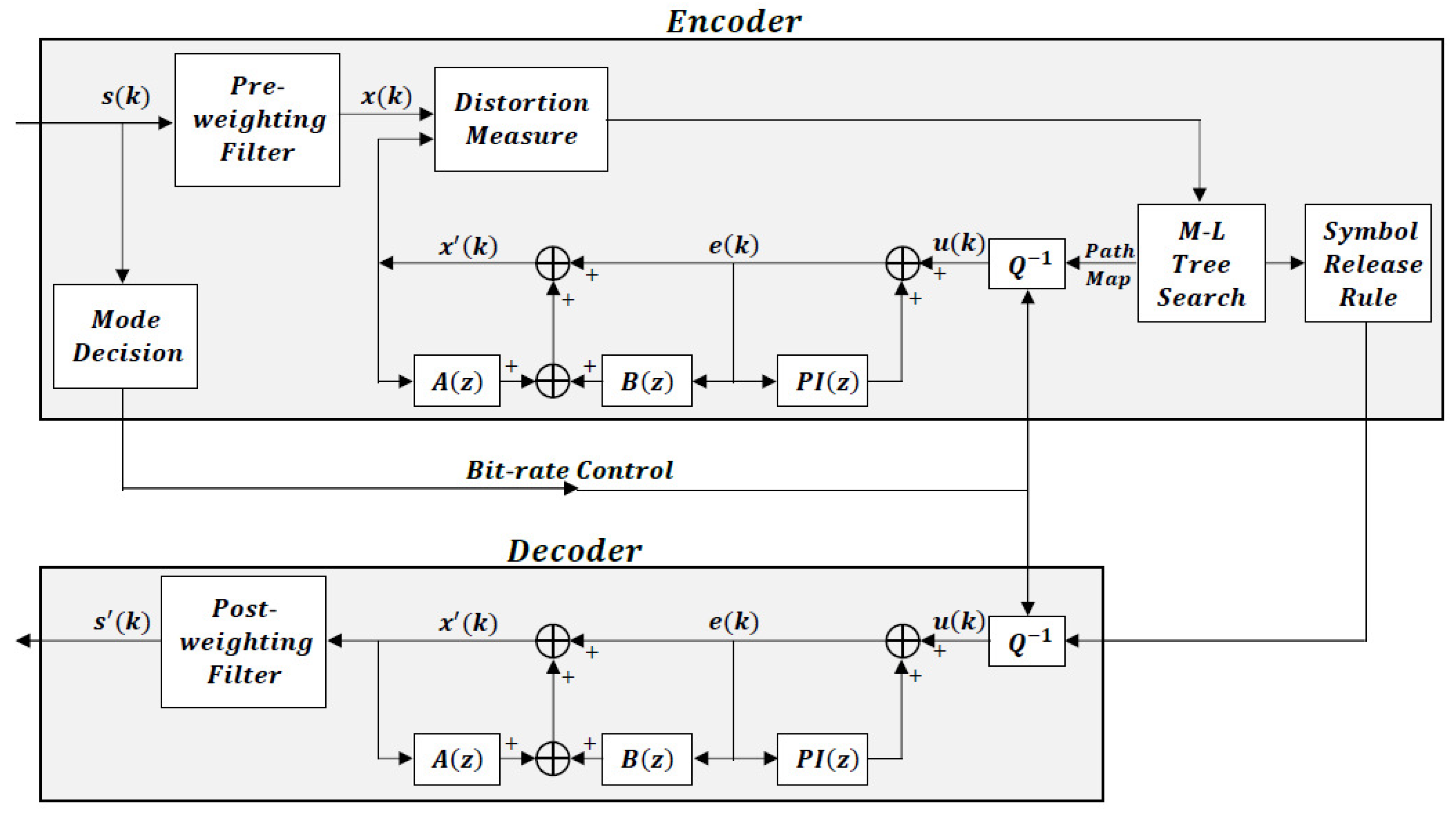
Figure 1 is the block diagram of the Multimode Tree Coder with backward pitch predictor and perceptual pre- and post-weighting filters, designated as MMT-WP. This diagram shows the basic structure of the codec and the locations of the several components.
We see from the figure that the codec involves both pole and zero short-term predictors and a long-term predictor . This combination is called a code generator in tree-coding. Additionally evident from the figure is a now classical analysis-by-synthesis loop involving a distortion measure and a tree search for the best excitation. The figure also shows the Mode Decision outside of the encoding loop and the new location of the perceptual weighting outside of the encoding and decoding sequence. These components and the others are developed in detail in subsequent sections.
4. G.727 DPCM Encoder
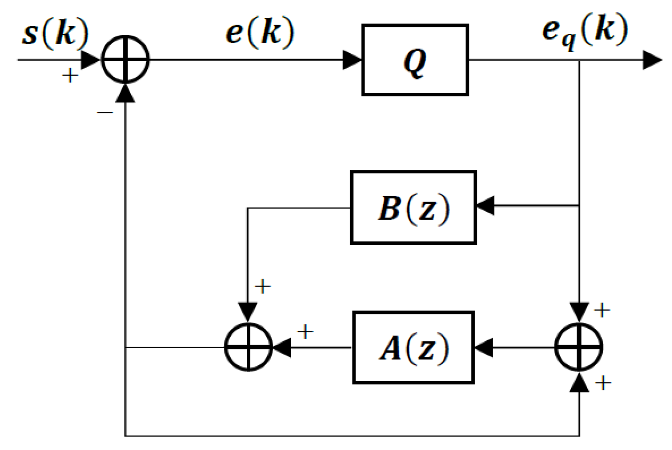
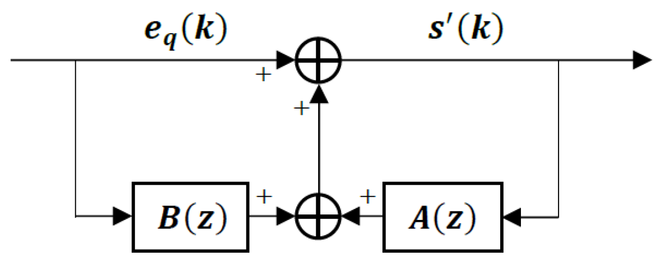
Differential pulse code modulation (DPCM) with an adaptive pole-zero short-term linear predictor is the basic structure of the ITU-T G.726 standard [24] and its embedded coding version G.727 [25,26]. Both codecs have selectable transmitted bit rates of 40, 32, 24, and 16 kbps from best to worst reconstruction quality. G.727 is an embedded codec so it has enhancement and core bits, and the coding rate is often specified in terms of enhancement and core bits/sample as (x,y), where x represents the total of the enhancement and core bits, and y refers to the number of core bits. Therefore, G.727 coding rates are (5,4), (5,3), and (5,2) for 40 kbps, (4,4), (4,3), and (4,2) for 32 kbps, (3,3) and (3,2) for 24 kbps, and (2,2) for 16 kbps. Figure 2 is a block diagram of the encoder and Figure 3 is a block diagram of the decoder. The specific structures and adaptation rules for and are developed in Section 4.1.
The quantizer is represented by Q in the figures and the quantizers and adaptation rules are described briefly in Section 4.2.
4.1. Short-Term Predictor
The short-term predictor is a 2-pole and 6-zero backward adaptive predictor. The two pole coefficients () of the predictor are adapted by [24,25]:
and
where
The six zero coefficients () of the predictor are adapted by:
for .
4.2. Adaptive Quantizers
The quantizers in G.726/G.727 adapt the step size to track the dynamic range of the prediction error signal. The step size is adapted according to two scale factors every sampling instant [24,25]. One scale factor, called the unlocked step size, , adapts as
where and the M parameters are multipliers that are greater than one for outer quantizer levels and less than one for the inner levels.
In addition to the unlocked step size, there is another step size in G.726/727, denoted as , that adapts more slowly. This step size adapts according to the logarithm of its value as well as the logarithm of . Defining , the adaptation rule is
5. Backward Pitch Predictor
To improve the performance of the G.726/727 codec structure, we add a long-term adaptive predictor to compensate for speaker pitch. The pitch predictor is a 3-tap backward pitch predictor, which is defined as [27,28]:
5.1. Backward Pitch Estimation
The pitch period at time instant k is estimated from previous reconstructed signal e. The autocorrelation function of e is calculated every 240 samples. In addition, when the previous pitch period increases one or decreases one and the shifted coefficients are not stable, the pitch period and pitch coefficients are initialized again by calculating the autocorrelation function . The pitch period is initialized by finding the peak of between and , and then is recursively updated. The estimate of the autocorrelation function, , is obtained from the following recursions [3,28]:
where . The pitch period is updated by:
5.2. Backward Pitch Coefficients Calculation
After obtaining the pitch period , the pitch coefficients can be calculated as follows. The initial pitch coefficients of each block are calculated using a Wiener–Hopf equation [27,28]:
where . When pitch coefficients of each block are initialized, other pitch coefficients are recursively adapted using the equation:
where and , is the output of inverse quantizer, is the estimate of the variance of , and is the estimate of the variance of the output of pitch predictor . The estimated variances are calculated using Equation (10).
6. Tree-Coding
Tree-coding is a type of analysis-by-synthesis coding structure similar to Code-Excited Linear Prediction (CELP), but differs from CELP in that the codebook has a tree structure and the delay in the analysis-by-synthesis procedure is less [29]. Tree-coding is a natural way to incorporate the analysis-by-synthesis approach into backward adaptive codecs such as G.726/727, leading to expected performance improvements.
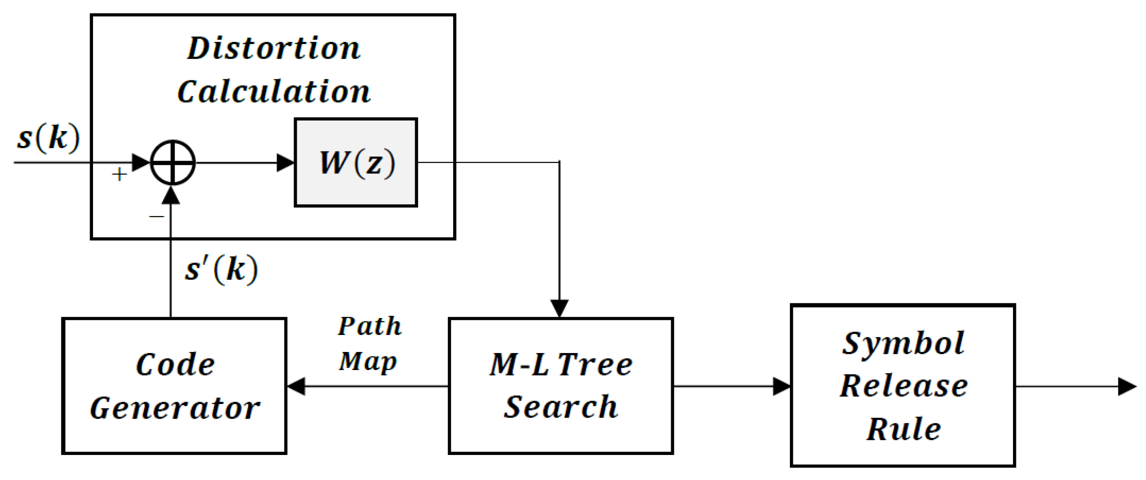
A block diagram of a tree coder for speech is shown in Figure 4. A tree coder consists of a Code Generator, a Code Tree (set of excitations), a Tree Search algorithm, a Distortion calculation, and a Path Map Symbol Release Rule. The Tree Search algorithm, in combination with the code generator and appropriate distortion measure, chooses the best candidate path to the tree depth L to encode the current input sample. The symbol release rule decides the number of symbols on the best path to transmit or release.
In tree-coding of speech, the terminology Code Generator refers to the structure that colors the code tree excitations and usually consists of a short-term predictor and a long-term predictor.
The tree code provides the excitation to the code generator to synthesize the reconstructed speech. To construct the tree, we must select the number of branches per node and the number and type of excitation values per branch. Then, the rate of the tree code in bits/sample is obtained from where is the number of branches/node and is the number of excitation values/branch. The selection of the number of branches/node and the number and values of the samples/branch are important design choices.
Once the code tree is designed, we need to search the tree for the best possible path to some depth L. If we have branches/node (corresponding to a 4-bit quantizer) and excitation value/branch, for a full search, we must search paths to depth L and there are L computations per path. Since performance often improves with search depth L, it is obvious that the computational load is immense, particularly since these sequences also must be passed through the recursive code generator. To reduce the computational complexity of searching the full tree to depth L with minimum cumulative distortion, it is common to use the (M,L) Tree Search algorithm [30]. This algorithm only retains M paths at each node. The minimum cumulative distortion path among the M depth-L paths is chosen. Then, the path map symbols according to this best path are released or transmitted to the decoder. Different path map symbol release rules are possible. All L path map symbols can be released and then the tree regenerated according to the (M,L) algorithm, or some number of symbols less than L can be released.
Most users of the (M,L) algorithm release only the first symbol along the best path, and then extend the M best paths with that symbol as their root. This is called the single symbol release rule (SSR) [31].
The distortion between the candidate output and the input sample is computed by filtering the error between them along the depth-L path through the perceptual error weighting filter similar to that used in CELP, which is of the form
The distortion values are stored along each searched path map. The path resulting in minimum cumulative distortion is encoded using the symbol release rule. However, the distortion calculation along each path obtained by filtering the error along depth-L path through the perceptual error weighting filter in Equation (15) is computationally expensive. Therefore, to reduce complexity, perceptual pre-weighting and post-weighting filters can be used, as we do here.
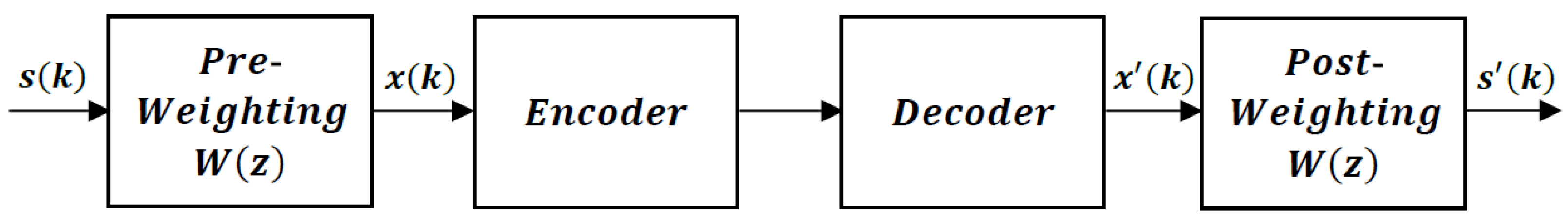
7. Perceptual Pre-Weighting and Post-Weighting
The computational complexity with the perceptual weighting filter inside the loop as in Figure 4 is computed as follows. If the computational complexity of is C operations, and is the number of children of each tree node for the n bits/sample tree, then the complexity of releasing one symbol is operations. Schuller, Yu, Huang, and Edler [32] have employed adaptive pre-filtering and post-filtering in lossless audio coding. They showed that lossless audio coding with pre- and post-filtering maintains high quality. In addition, Shetty and Gibson [33] employed perceptual pre-weighting and post-weighting in a G.726 ADPCM codec [24] and a modified AMR-NB CELP codec. They showed that the performance of lossy coding with pre- and post-weighting also improves over having no weighting. As shown in Figure 5, the computational complexity of our Multimode Tree Coder is reduced to operations for releasing one symbol using pre-weighting and post-weighting filters.
Let be the input speech, be the pre-weighted speech, be the pre-weighted speech output, and be the output speech after post-weighting. From Figure 5, the relation of and is
and the relation of and is
The design of the pre-weighting filter and post-weighting filter is to mask the reconstruction error at the output by the input spectrum. The spectral response of the perceptual weighting filter should have the form of that shown in Equation (15).
However, the input spectrum information is not available at the decoder in our codec; so our post-weighting filter uses the pole-zero coefficients from the backward adaptive predictor. The post-weighting filter is of the form,
where ’s are pole coefficients and the ’s are zero coefficients, and we have added an additional denominator term mainly to tune the spectral tilt.
To choose the weighting filter parameters, , , and , in Equation (18), experiments were conducted to match the frequency response of the perceptual post-weighting filter generated with 5th order linear prediction coefficients calculated from the input, Equation (19),
with the frequency response of the filter generated with the ADPCM predictor coefficients. After experimentation, the parameters were chosen to be , , and in both pre- and post-weighting filters.
8. Voice Activity Detection (VAD) and Mode Decision
Most high-performance codecs today use some approach to VAD. Usually these methods are quite complex, such as in [8]. Our approach is much simpler since the codec is backward adaptive and low delay and relies more on the available codec parameters. The VAD method developed here is an entirely new, simplified approach.
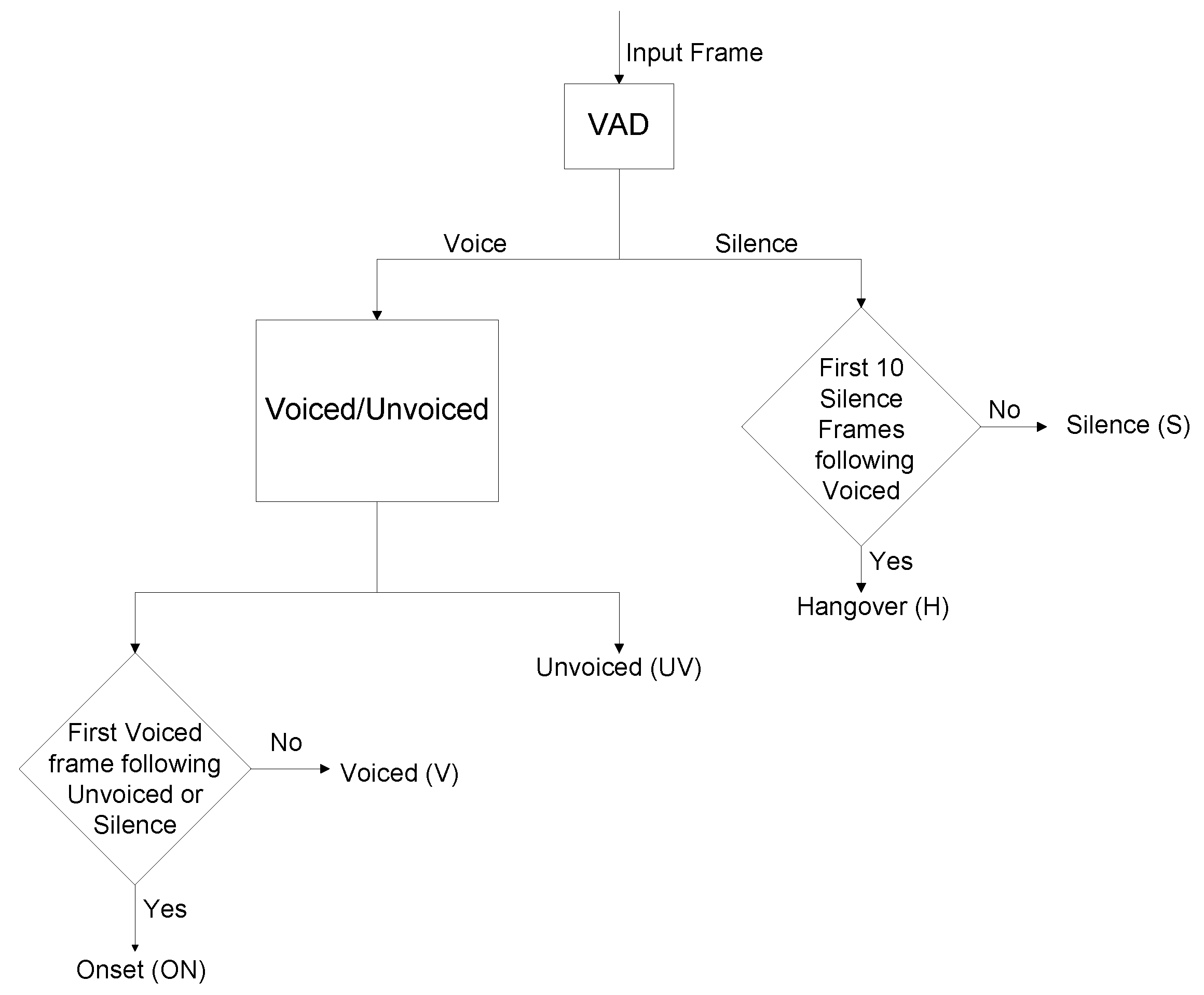
The flow chart of our mode decision is shown in Figure 6. The mode decision is a low-delay, low-complexity method based on the ADPCM coder state parameters, unlocked scale factor and long-term average magnitude of weighted quantization level , along with the absolute magnitude of each frame and zero crossing rate. The input to the mode decision is a speech frame consisting of 40 samples of 8 kHz narrowband speech, and the output is the classification of the frame among one of these five modes: Voiced (V); Onset (ON); Unvoiced (UV); Hangover (H); and Silence (S). In the following, the term “Voice” is used to denote all non-silence speech and the term “Voiced” is used to denote the Voiced (V) mode of speech. The input frame of speech is first classified into Voice/Silence by Voice Activity Detection (VAD) before further classification into five modes.
The unlocked scale factor is updated for the adaptive quantizer in the G.727 ADPCM coder. The long-term average magnitude of weighted quantization level is calculated. The absolute magnitude of each frame is widely used in VAD algorithms. It is computed for each frame i as follows,
where s is the normalized input speech signal, normalized to input speech power, and N is the length of a speech frame. The number of zero-crossings is widely used for voiced and unvoiced classification, which is defined as:
with the sign function returning depending on the sign of the operand.
The unlocked scale factor , long-term average magnitude of weighted quantization level , and frame energy are high during Voice sequences and low during Silence sequence. Therefore, the three parameters are compared against threshold values computed for each parameter to make a Voice Activity Detection decision. If or is greater than its threshold, or , and is greater than the threshold , then the frame is marked as Voice. If and are smaller than their thresholds, and , and the status continues for at least 15 frames, then the frame is marked as Silence.
After Voice Activity Detection, each frame should be further classified into Voiced (V), Onset (ON), Unvoiced (UV), or Hangover (H). For the frame marked as Voice, it will be further classified into Unvoiced (UV), Onset (ON) or Voiced (V). If , , and are smaller than their thresholds, , , and , and is greater than the threshold , the frame is classified as Unvoiced (UV). Otherwise, it is classified as Voiced (V). The first Voiced frame following Unvoiced or Silence frame is marked as Onset (ON). For the frame marked as Silence, it will be further classified into Silence (S), or Hangover (H). The first ten Silence frames following Voiced are marked as Hangover (H). Otherwise, it is marked as Silence (S).
Table 1 shows the details of the test sequences. The test sequences are all longer than one sentence, and there are four female and four male speakers. The sentences were chosen to cover a wide range of difficult-to-code phonemes and words. The sentence, “We were away a year ago,” is included since it is almost totally voiced, without unvoiced sounds or silence. These test sequences are taken from a standard ITU-T speech test data set [34] for standardized speech codecs. Their bandwidth is 300 to 3400 Hz, and they are sampled at 8000 samples/sec. Each sample is represented as a 16 bit linearly quantized word. The terminology dBov is the dB level relative to the overload of the system.
The relative frequency of these classifications according to modes using our algorithm on each sentence are shown in Table 2.
The thresholds chosen by experiment in the design presented here are:
- = 0.04
- = 5
- = 0.6
After the VAD decision, then the voicing decisions use the thresholds:
- = 0.33 of average
- = average
- = 0.3 of average
where the averages are over a frame, and these are updated on a frame-by-frame basis. was not used in our final design, although it can be used to fine tune unvoiced decisions if needed. It is important to notice that the threshold values given here are all normalized values, being normalized to the power level of the input speech levels. This is as typical in VAD and mode decision rules used in other codecs such as AMR. Therefore, these values are robust to variations in input speech power and across different utterances. The VAD and Mode not only impact reconstructed speech quality but also the transmitted bitrate.
9. Zeros in the Short-Term Predictor
The G.726/727 codecs have 2 poles and 6 zeros. When these codecs were being standardized, the order of the all-pole predictor was reduced so that stability tests could be easily performed and the predictor stabilized, but the zeros were needed to compensate for any loss in prediction performance from using only 2 poles but without risking instabilities. However, there are other important reasons for including zeros in a backward adaptive tree-coding structure.
First, it is well known that when estimating the parameters of an autoregressive (AR) sequence in additive noise, the estimation procedure should include zeros [35,36]. The inclusion of zeros can make the estimation more accurate and can reduce the flattening of the estimated spectral envelope of the AR model.
Second, rate distortion theory indicates that for optimal encoding using the mean squared error distortion measure, the code generator should include zeros as well as poles when achieving small distortion [29].
Third, from studies of backward adaptive prediction with a quantizer in the loop, it is known that an all-pole model can end up tracking itself rather than the input speech signal. The inclusion of zeros in the adaptive predictor can prevent this behavior and can couple the backward adaptive predictor to the codec input signal more directly [37].
For all these reasons, we include zeros in our short-term backward adaptive predictor structure.
10. Performance of the Multimode Tree Coder
10.1. The Bitrate of the Multimode Tree Coder
The bitrate of the Multimode Tree coder is controlled by the mode decision output. The mode decision output, the frame header, is coded with 2 bits. The two header bits, 00—S, 01—UV or H, 10—V, and 11—ON, are used to specify the mode of each frame. Since the frame length for the narrowband Multimode Tree coder is 5 msec, the bitrate of the header is 0.4 kbps.
Since we use the quantizer of G.727 in the code generator, the bitrate of UV, V, ON, and H can be 16, 24, 32, or 40 kbps. In addition, G.727 is an embedded ADPCM coder. Therefore, the number of core bits and enhancement bits can be adjusted as well. For simplicity, we do not use enhancement bits in our experiments. In the tree coder, M is 4 and L is 10 for the M-L Tree Search algorithm.
To lower the average bitrate, the Comfort Noise Generator (CNG) motivated by the CNG of AMR-NB [38] is used for Silence (S) mode. In the CNG, the pole-zero predictor coefficients from the short-term predictor are averaged between each transmission frame and encoded every 15th frame. The absolute magnitude of each frame is averaged and transmitted every 8th and 15th frames. The averaged absolute magnitude is transmitted with 5 bits, the averaged pole coefficients are transmitted with 7 bits, and the averaged zero coefficients are transmitted with 5 bits. Since there are 2 pole coefficients, 6 zero coefficients and 2 averaged absolute magnitude transmitted for every 15 frames, the total transmitted bits is 54 bits. Therefore, the bitrate for Silence (S) mode is 0.72 kbps.
10.2. Performance with Different CNG Codes
We compare the PESQ of the MMT with perceptual pre- and post-weighting and backward pitch prediction (MMT-WP) for Voiced (V) and Onset (ON) using 3 core bits/sample and Voiced (V) and Onset (ON) using 2 core bits/sample. The Unvoiced (UV) and Hangover (H) are coded at 2 core bits/sample.
The PESQ-MOS [4] results of the MMT-WP for narrowband sequences using 2 core bits/sample on Voiced, Onset are shown in Table 3. Compared with the results of 3 core bits/sample for Voiced and Onset in Table 4, the PESQs of 2 core bits/sample for Voiced and Onset in Table 3 are lower than those in Table 4 since the bitrate is lower. However, comparing the performance of MMT with weighting and pitch predictor with the performance of MMT without pitch prediction from prior studies, the PESQ for 2 bits/sample increases more than the PESQ for 3 bits/sample on Voiced and Onset. It shows that the pitch predictor is very important when the bitrate is low.
11. Estimated Computational Complexity of MMT-WP
The estimated computational complexity of the several components of MMT-WP is shown in Table 5. Table 2 shows the mode decision results of each sequence. Based on the mode decision, the estimated computational complexity of MMT with pre- and post-weighting and pitch filter is shown in Table 6. When the sequence is 100% voiced, the computational complexity for MMT-WP is the worst case. Based on the per component estimated computational complexities in Table 5, the worst computational complexity for MMT-WP including Mode decision, tree coder, the G.727 decoder, pre- and post-weighting, and pitch predictor is 4.83 WMOPS. Since “we were away” is a fully voiced sentence with no silence, the computational complexity for this sentence is the worst case. The probability of silence for sequences af1s01m af1s02, af1s03, am1s01, am1s02, and am1s03 is about 58%. Since the computational complexity for silence is 0.08916 WMOPS, the computational complexity of these sequences is less than half of the worst computational complexity for “we were away” in Table 6.
12. Comparison Codec Selection
The AMR-NB/WB codec is a workhorse in digital cellular and VoIP applications. It has outstanding reliability and consistent performance across many platforms and networks. The newer Enhanced Voice Services (EVS) codec was standardized in 2014 with the goal of not only improving performance for narrowband and wideband applications but also to develop a codec for superwideband applications and to improve performance for music and mixed inputs in conversational speech and to add stereo audio, plus improved VoIP performance through jitter buffer management, better packet loss robustness, and additional input and output processing [11]. All this improved functionality came at the price of greatly increased complexity and longer encoding/decoding delay. The EVS codec is at least twice as complex as AMR-WB and 5 times more complex than the AMR-NB codec used in the comparisons here [39].
It is well established that the increased complexity does yield better performance than AMR-NB/WB [40], so it is a given that the EVS codec outperforms both AMR-NB/WB and our MMT-WP codec in terms of speech quality at the same bitrate. However, many applications that focus on NB speech, such as we do here, do not need all the functionality in the EVS codec and the increased complexity and latency is not worth the improved speech-coding performance over AMR-NB/WB, which performs very well. Since AMR-NB/WB is widely installed and used, and has much reduced complexity and slightly reduced latency than EVS, AMR-NB/WB is the codec we compare to since our first priorities are much reduced complexity and latency.
13. Performance Comparisons of MMT-WP with Other Codecs
Table 7 shows the PESQ, average bitrate, algorithmic delay, and computational complexity comparison of the MMT-WP codec with AMR-NB and G.727 [3]. We see that the MMT-WP codec can produce the same output speech quality as G.727 but at much lower bit rates. Furthermore, the MMT-WP codec has much lower complexity and much lower delay than AMR-NB while producing the same output speech quality, albeit at higher bit rates.
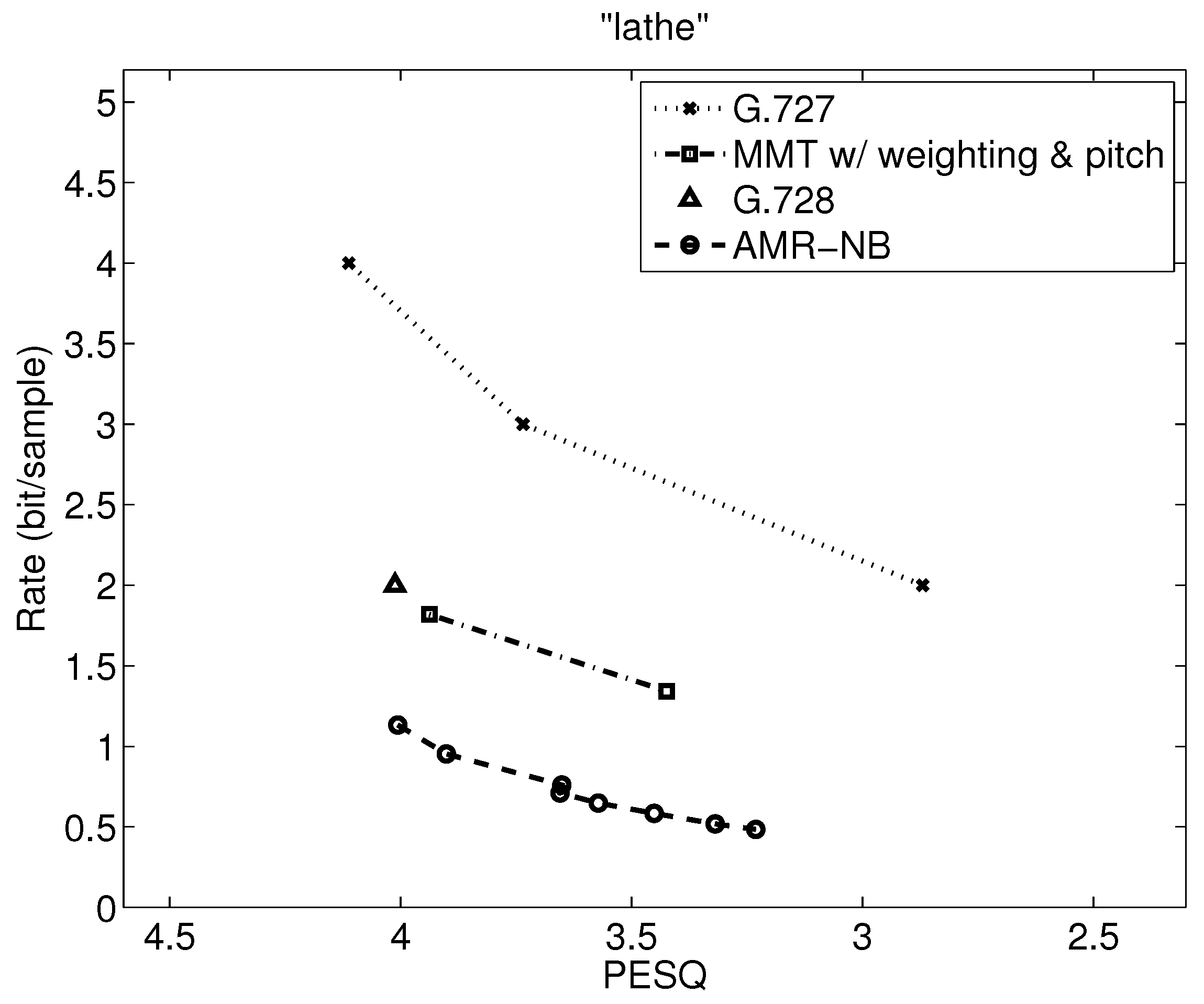
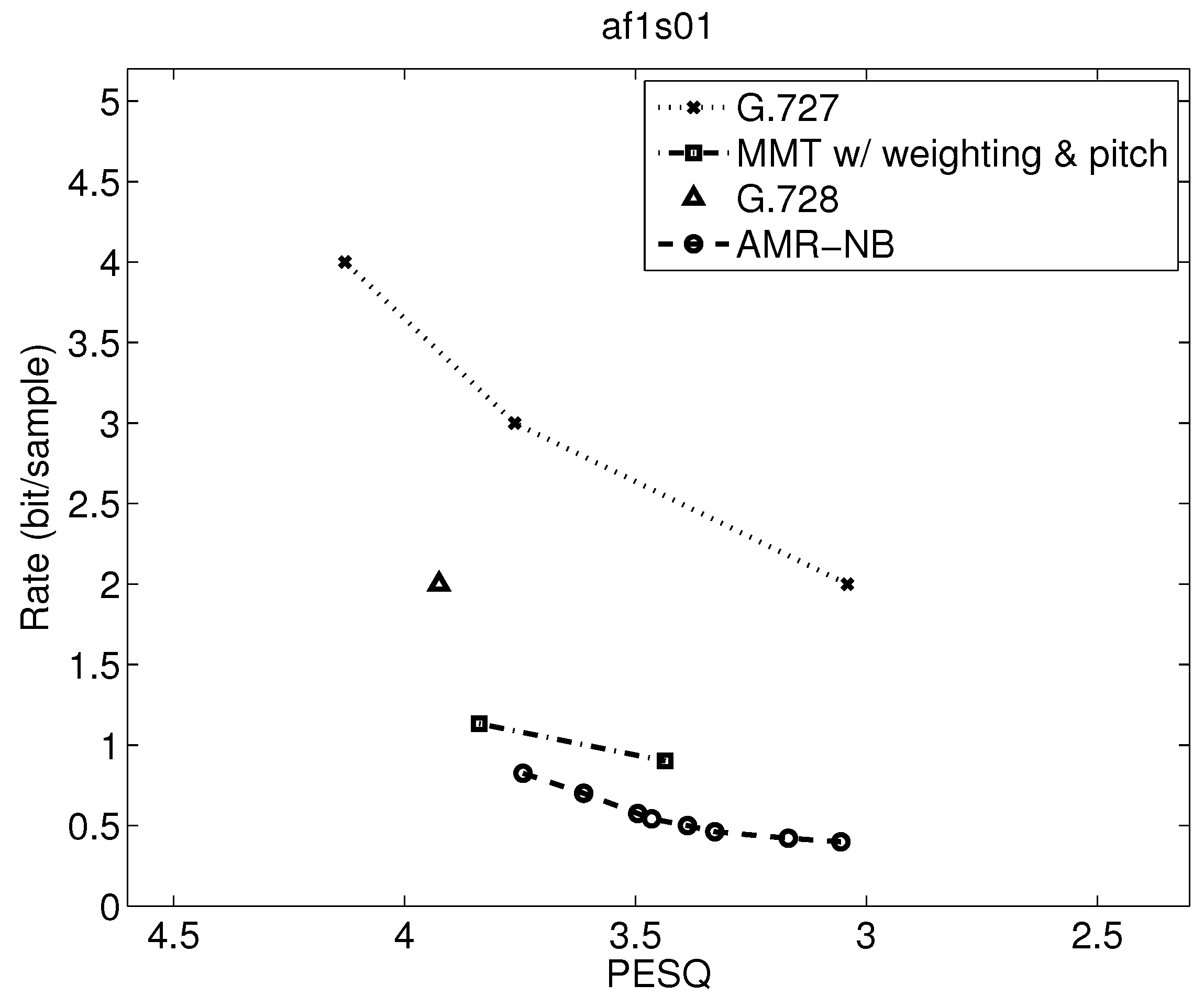
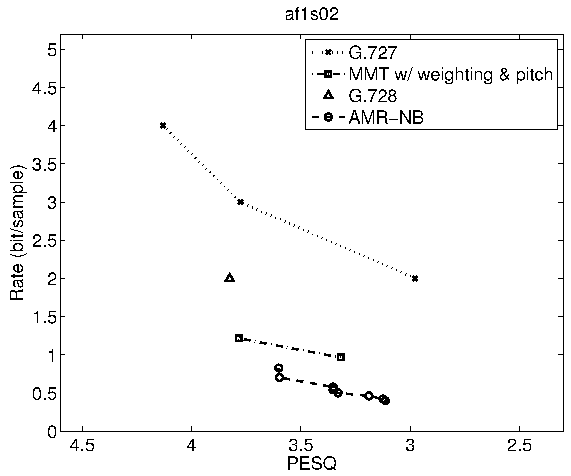
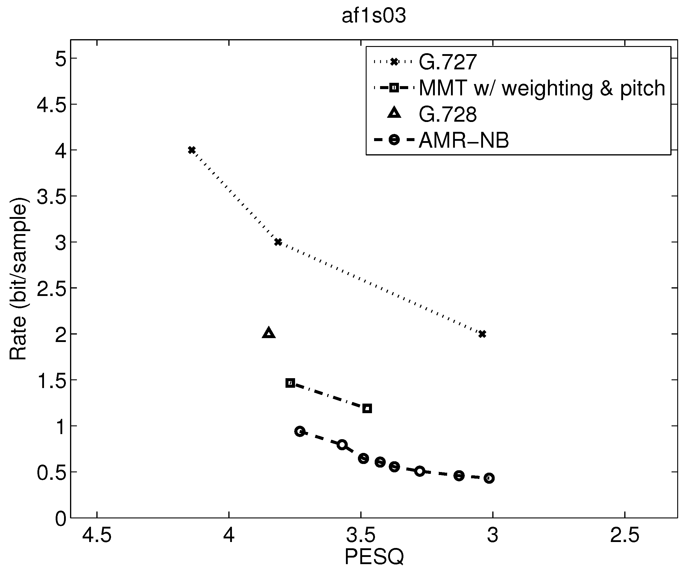
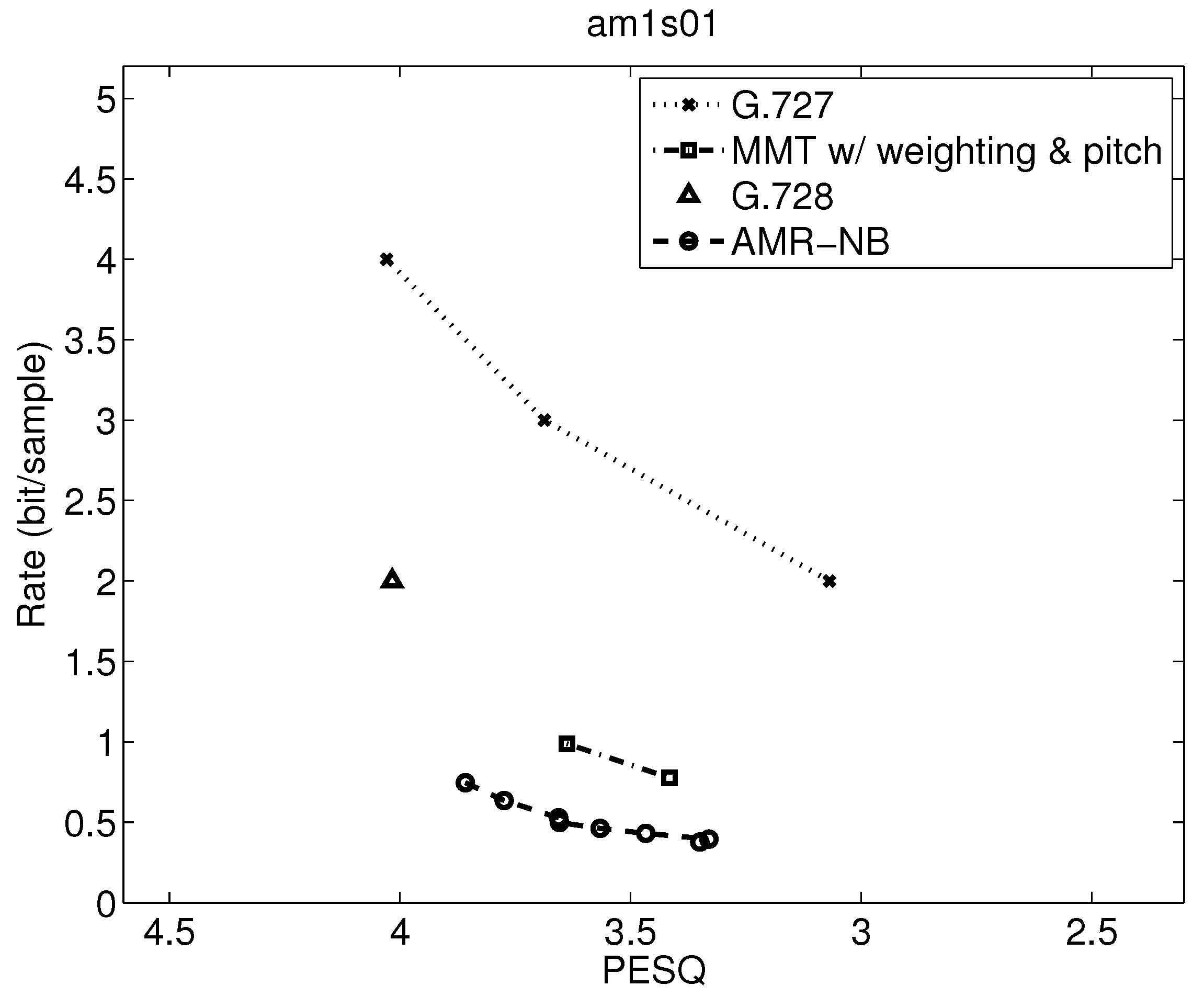
Table 7 shows the range of PESQ-MOS, bitrate, delay, and computational complexity over the utterances examined, but a closer examination can indicate where the variations are from. Operational rate distortion functions allow a more detailed performance comparison of possibly competitive voice codecs [41]. Figure 7, Figure 8, Figure 9, Figure 10, Figure 11, Figure 12, Figure 13 and Figure 14 show PESQ and average bitrate of different speech codecs on 8 clean English sequences described in Table 1.
Compared to AMR-NB, the PESQs of MMT-WP with weighting and pitch predictor using 3 bits/sample for Voiced and Onset (the highest bitrate of MMT) are comparable with the PESQs of AMR-NB at 12.2 kbps (the highest bitrate of AMR-NB). Even though the average bitrate of MMT-WP is 0.25–1.5 bit/sample higher than that of AMR-NB, the delay and computational complexity of MMT are significantly lower than those of AMR-NB. Furthermore, the algorithmic delay of MMT-WP is 6.125 msec while that of AMR-NB is 25 msec. Thus, the delay of MMT-WP is about a quarter of AMR-NB. The worst computational complexity of MMT-WP with weighting and pitch predictor is 4.83 WMOPS while the worst computational complexity of AMR-NB is 16.7 WMOPS. Therefore, MMT-WP saves about 70% in computational complexity.
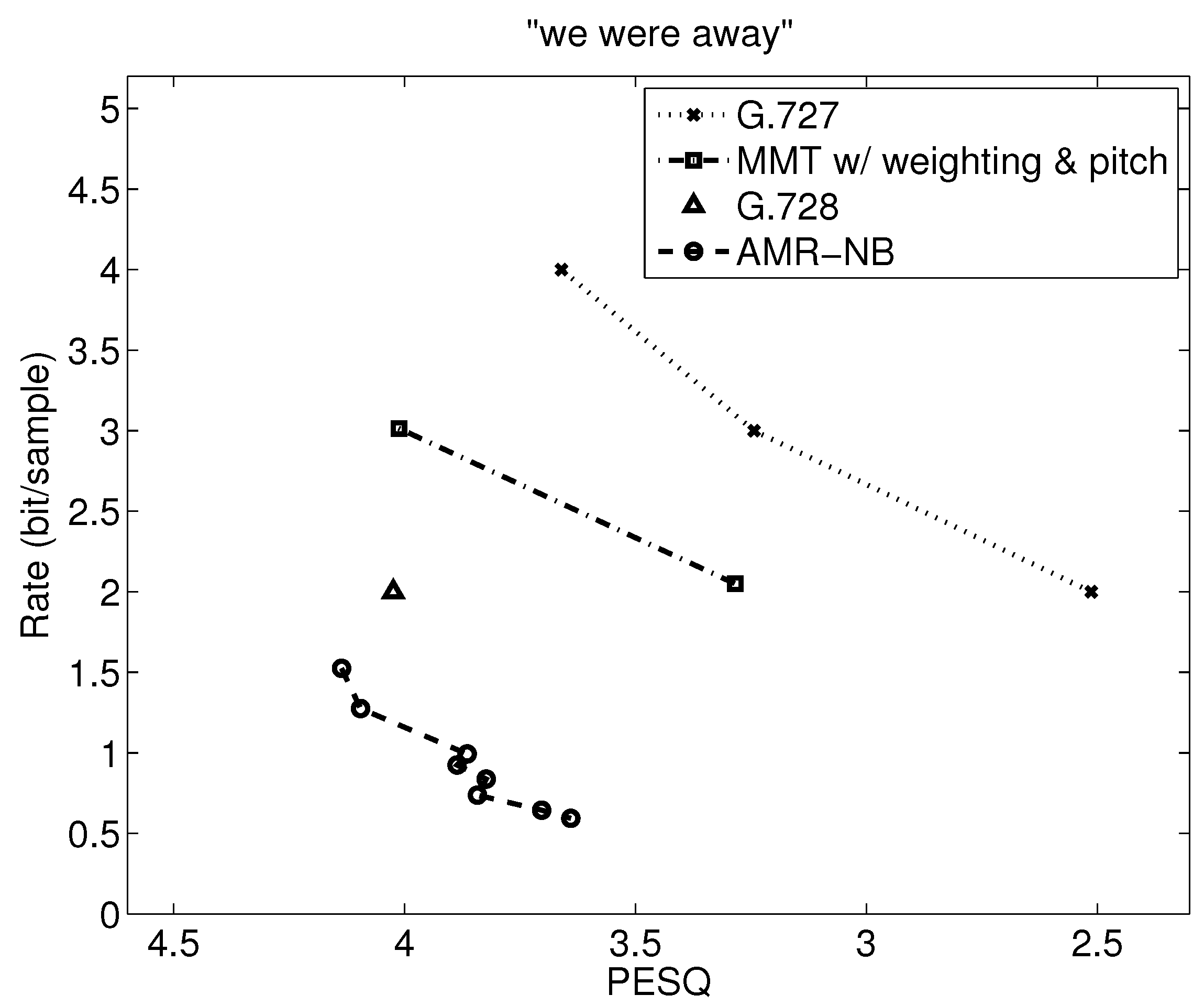
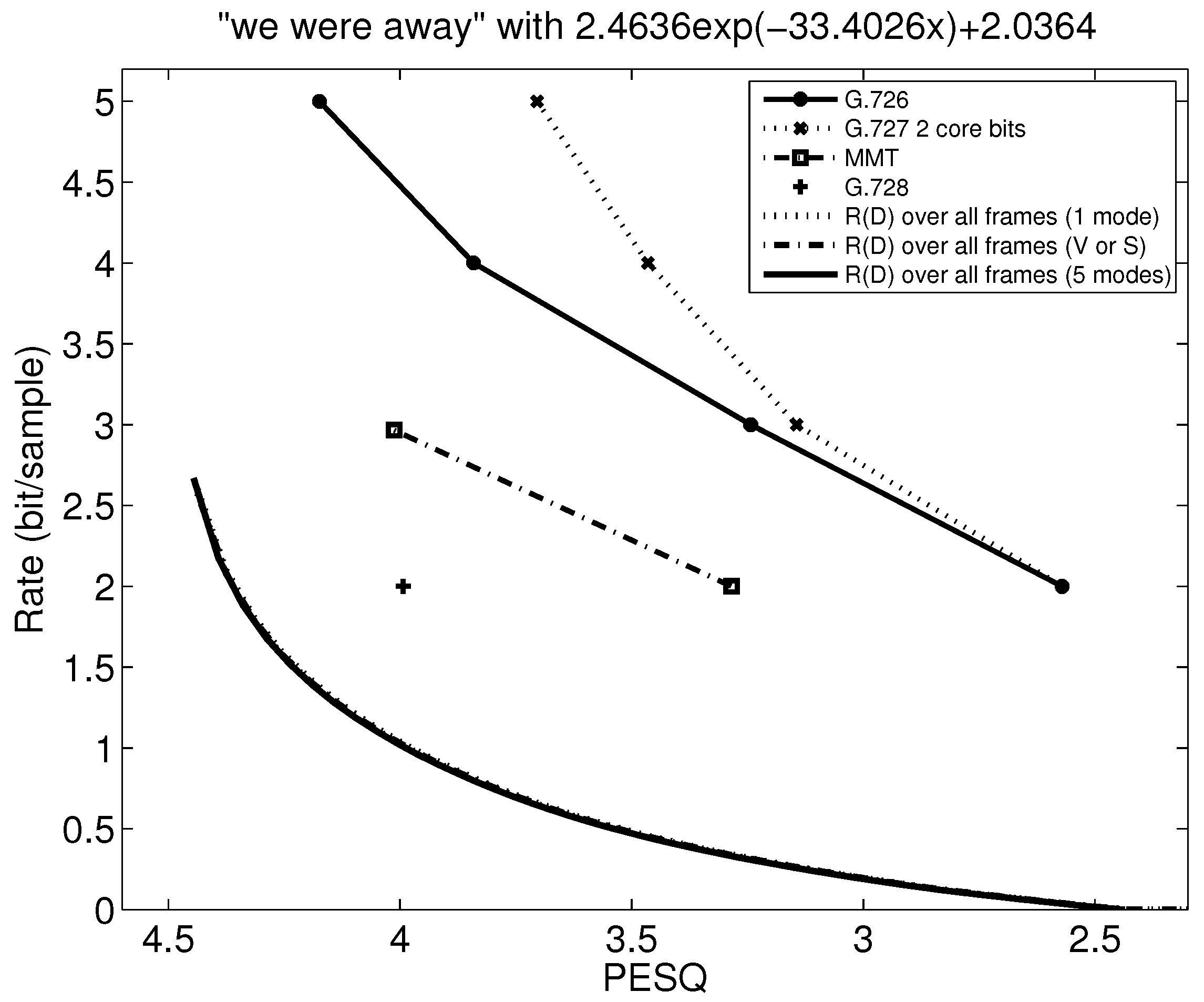
Referring to Figure 8 and comparing MMT-WP to G.727 for the sequence “we were away,” the PESQ for G.727 at 16 kbps is 2.513 while the PESQ for MMT with weighting and pitch predictor at 24 kbps is 4.012. Moreover, the PESQ for G.727 at 32 kbps is 3.66, which is lower than the PESQ for MMT-WP at 32 kbps. This shows that MMT with weighting and pitch predictor saves about 1 bit/sample when PESQ is comparable with G.727.
Analyzing Figure 7 and Figure 8 to compare MMT-WP with AMR-NB, we see that there is a relatively constant gap of just under 1 bit/sample between MMT-WP and AMR-NB for “lathe” with the same PESQ-MOS values, and this gap widens to 1.5 to almost 2 bits/sample for “we were away” since the MMT-WP loses any rate reduction produced by VAD/CNG because “we were away” is all voiced.
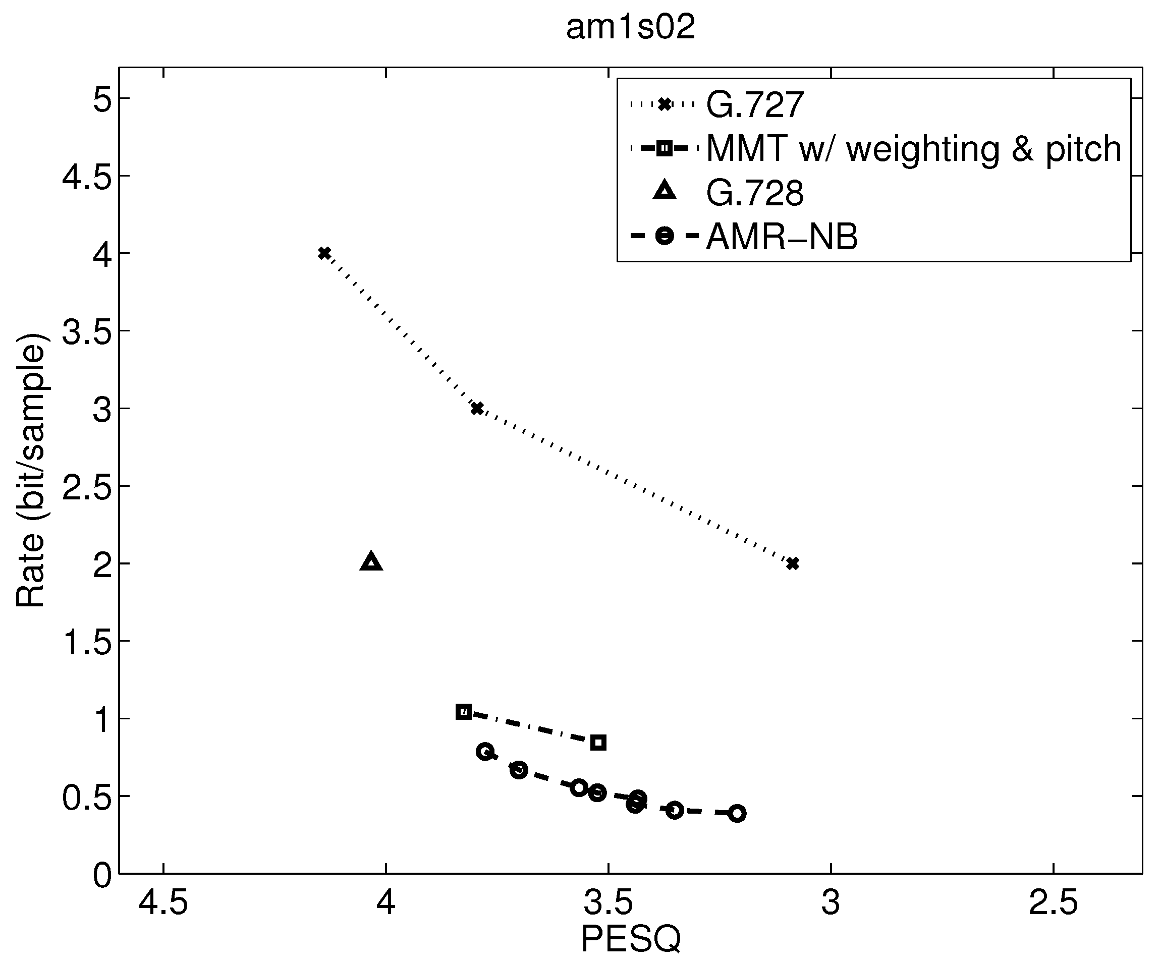
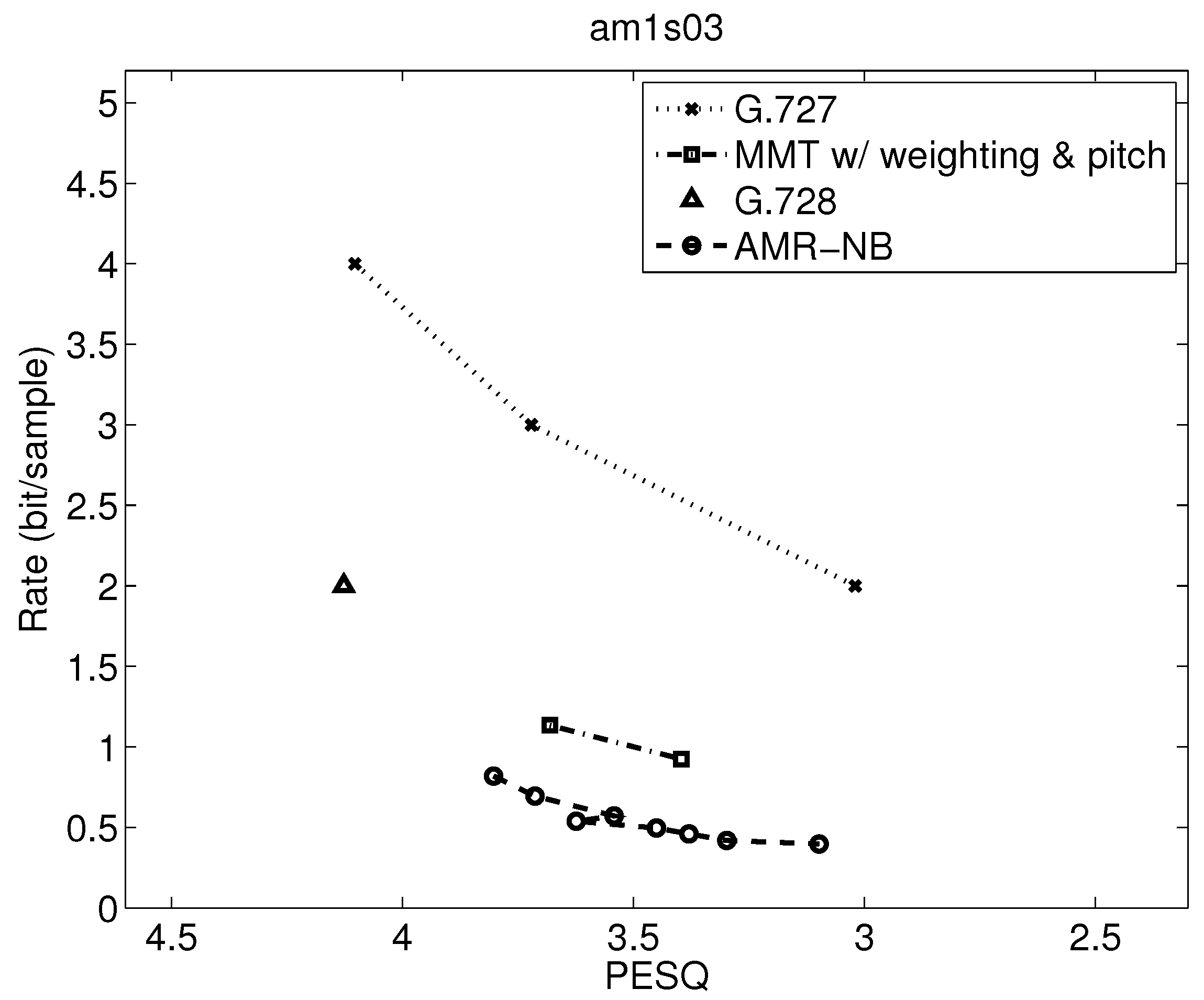
Comparing results in Figure 9, Figure 10, Figure 11, Figure 12, Figure 13 and Figure 14, where the first three figures are for female speakers and the latter three are for male speakers, we can see some further trends. First, it is evident that the gap between MMT-WP and AMR-NB is narrowed to less than 0.5 bit/sample for these sentences for the desirable quality range shown. Additionally, the gap between these two codecs varies somewhat for these six test sequences.
Furthermore, for the MMT-WP codec, the female speakers have a slightly higher bitrate for the same performance than the male speakers. This does not appear to be the same for the AMR-NB codec where the rate distortion performance is about the same for female and male speakers. The small difference in performance between female and male speakers for the MMT-WP codec is likely due to the increased number of pitch periods for female speakers compared to male speakers which requires an increased use of the long-term prediction for the female speakers. Our backward adaptive pitch tracking and pitch coefficient adaptation may need further optimization, but this is not certain nor easy.
The operational rate distortion functions in the figures not only include G.727, AMR-NB, and MMT-WP but also G.728 [42]. G.728 is a standardized codec for operation at the single bitrate of 16 kbps but without voice activity detection and comfort noise generation. The use of VAD/CNG will lower the bits/sample of G.728 further. We include G.728 combined with the AMR-NB VAD/CNG in the studies comparing MMT-WP and AMR-NB with theoretical rate distortion bounds in Section 14.
The operational rate distortion performance curves shown in Figure 7 through Figure 14 illustrate that average performance comparisons between codecs over various test sequences may not capture the possibly significant variation around the average. Studies of individual sequences as done here, while requiring substantial effort, are necessary to evaluate the actual performance range of codecs. This insight foreshadows the approach necessary to obtain meaningful rate distortion bounds.
14. Comparison with Rate Distortion Bounds
Rate distortion functions provide the optimal performance theoretically attainable (OPTA) for compressing a given source with a selected distortion measure [41]. To derive such bounds, we need a good source model of a physical source and a meaningful distortion measure. Both have been stumbling blocks to obtaining useful rate distortion bounds.
Models averaged over many sentences do not allow such bounds to be developed because an average source cannot produce a lower bound since one of more of the sources in the average will almost certainly have performance that is better than the average bound developed. Thus, a new model needs to be obtained for each sentence or utterance considered. Additionally, the distortion measure challenge is that it must be analytically tractable and physically meaningful. Most rate distortion functions have been derived for mean squared error or Hamming distortion measures.
Gibson and Hu used existing rate distortion functions for autoregressive sources for mean squared error distortion but extended those results using composite source models [29] and conditional rate distortion theory [43] to generate good source models for speech [5,44]. For the distortion measure, they experimentally obtained a mapping from mean squared error into PESQ-MOS. Thus, the need for an accurate source model and a meaningful distortion measure were both addressed.
Three models for each sentence are obtained. One model is averaged over the entire utterance, one model that has two modes, voiced and silence, and a third model that has 5 modes, voiced, unvoiced, silence, onset, and hangover. The conditional rate distortion bound is derived for each subsource, along with the probability of that subsource, and these conditional rate distortion bounds are combined as indicated by conditional rate distortion theory [5,43].
The mapping from MSE to PESQ-MOS is generated for each utterance using waveform codecs which try to track the time domain waveform but also allow the PESQ-MOS to be found. The waveform codecs need to have a range of coding rates so a mapping can be obtained. G.727 is one such codec and is one of the codecs used by Gibson and Hu [5].
The details of producing the composite source models and the MSE to PESQ-MOS mappings are left to the monograph by Gibson and Hu [5]. We use their approach here to develop rate distortion bounds for two of our sentences, “A lathe is a big tool” and “We were away a year ago”.
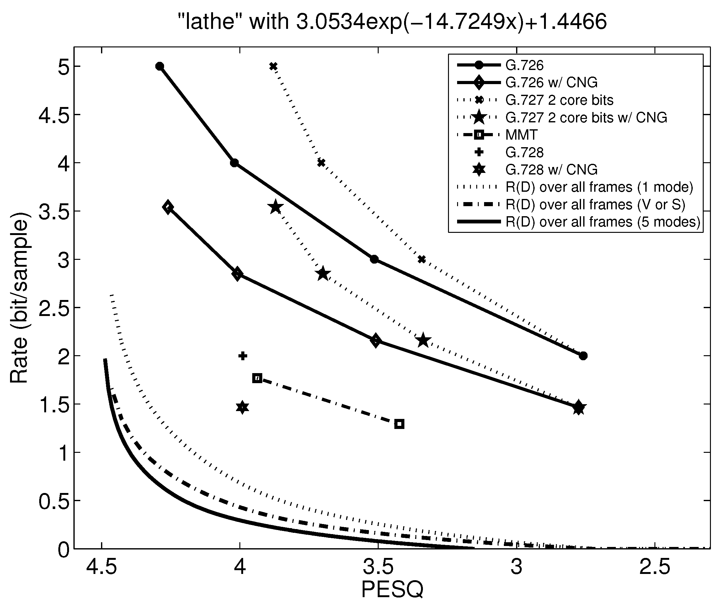
Figure 15 and Figure 16 show the PESQ and rate performance of G.726, G.727, G.728, and MMT with weighting and pitch predictor, and the rate distortion bounds for three different source models. In Figure 15, compared with the G.726 PESQ-rate performance curve, MMT with weighting and pitch predictor is about 0.8 bit/sample lower than G.726 when the PESQ are comparable. Compared with the rate distortion bounds using the 5 modes source model, MMT-WP is still 1.5–2 bits/sample above the theoretical rate distortion bound.
Results for G.728 and G.728 with VAD/CNG are also shown in Figure 15 and Figure 16. We see that G.728 at 2 bits/sample achieves a PESQ-MOS of near 4.0 for both sentences. When VAD/CNG is used with G.728, 0.5 bit/sample is saved for “lathe” as seen in Figure 15, but from Figure 16, there is no reduction in rate when using VAD/CNG with G.728 because “we were away” is an all-voiced sentence.
15. Conclusions
The performance evaluations reveal that the design decisions of moving the perceptual weighting outside of the analysis-by-synthesis loop can, not only perform well, but also result in a substantial reduction in algorithmic complexity. The sequentially adaptive long- and short-term predictors coupled with the small look ahead of the tree coder keeps the latency low as well. The use of VAD plus CNG for multimode coding pushes the bitrate down for utterances with about 50% silence, as is relatively common. Therefore, the Multimode Tree Coder with sequentially backward adaptive short- and long-term prediction and perceptual pre- and post-weighting filters can reduce complexity and latency in those applications where the reasonable performance penalty compared to increased complexity and latency codecs can be absorbed.
Further research that incorporates a more advanced sequentially adaptive prediction algorithm, such as recursive least squares, could provide substantial performance improvements while maintaining low latency with slightly increased complexity. Codecs built around the MMT-WP using a two-band codec structure can extend the approach to wideband speech and is an area of future research. In fact, given the combination of performance, low latency, and low complexity provided by the MMT-WP codec for narrowband speech, it is natural to consider extending the approach to wideband speech-coding. One such initial study split the wideband speech, usually 50 Hz to 7 kHz, into two bands using the quadrature mirror filters used in G.722 [45] and then coded the low band with an early version of the codec described in the current paper and coded the upper band using tree-coding with the upper band ADPCM coding of G.722 [46].
Improved performance of the above suggested wideband codec structure could be obtained at the cost of increased complexity using a recursive least squares adaptation of a higher order short-term predictor as in [30] and in [47], particularly in the low band. Low latency would still be retained.
A second possible approach is to filter the input 50 Hz to 7 kHz into the bands 50 to 6400 Hz and 6400–7000 Hz as in AMR-WB and code the lower band with a reoptimized version of the current MMT-WP codec. A new coding approach would need to be found for the high frequency band.
Author Contributions
All authors contributed equally to all aspects of this work. All authors have read and agreed to the published version of the manuscript.
Funding
This research received no external funding.
Institutional Review Board Statement
Not applicable.
Informed Consent Statement
Not applicable.
Data Availability Statement
Not applicable.
Acknowledgments
Conflicts of Interest
The authors declare no conflict of interest.
References
- Atal, B.S.; Schroeder, M.R. Adaptive predictive coding of speech signals. Bell Syst. Tech. J. 1970, 49, 1973–1986. [Google Scholar] [CrossRef]
- Jayant, N.S.; Noll, P. Digital Coding of Waveforms: Principles and Applications to Speech and Video; Prentice Hall: Hoboken, NJ, USA, 1984. [Google Scholar]
- Li, Y.-Y.; Gibson, J.D. Multimode Tree Coding of Speech with Backward Pitch Prediction and Perceptual Pre- and Post-weighting. In Proceedings of the the 46th Annual Asilomar Conference on Signals, Systems, and Computers, Pacific Grove, CA, USA, 4–7 November 2012. [Google Scholar]
- ITU-T Recommendation P.862; Perceptual Evaluation of Speech Quality (PESQ), an Objective Method for End-to-End Speech Quality Assessment of Narrow-Band Telephone Networks and Speech Codecs. ITU: Geneva, Switzerland, 2001.
- Gibson, J.D.; Hu, J. Rate distortion bounds for voice and video. Found. Trends Commun. Inf. Theory 2013, 10, 379–514. [Google Scholar] [CrossRef]
- Gibson, J.D. Speech Coding for Wireless Communications. In Mobile Communications Handbook; CRC Press: Boca Raton, FL, USA, 2012. [Google Scholar]
- Gibson, J.D. Speech compression. Information 2016, 7, 32. [Google Scholar] [CrossRef] [Green Version]
- ITU-T Recommendation G.729; Coding of Speech at 8 kbit/s Using Conjugate-Structure Algebraic-Code-Excited Linear Prediction (CS-ACELP). ITU: Geneva, Switzerland, 2007.
- 3GPP. Mandatory Speech Codec Speech Processing Functions; Adaptive Multi-Rate (AMR) Speech Codec; Transcoding Functions; TS 26.090; 3rd Generation Partnership Project (3GPP): Sophia Antipolis, France, 2011. [Google Scholar]
- 3GPP. Speech Codec Speech Processing Functions; Adaptive Multi-Rate-Wideband (AMR-WB) Speech Codec; Transcoding Functions; TS 26.190; 3rd Generation Partnership Project (3GPP): Sophia Antipolis, France, 2011. [Google Scholar]
- Dietz, M.; Multrus, M.; Eksler, V.; Malenovsky, V.; Norvell, E.; Pobloth, H.; Miao, L.; Wang, Z.; Laaksonen, L.; Vasilache, A.; et al. Overview of the EVS codec architecture. In Proceedings of the IEEE International Conference on Acoustics, Speech, and Signal Processing (ICASSP’15), South Brisbane, QLD, Australia, 19–24 April 2015. [Google Scholar]
- Kankanahalli, S. End-To-End Optimized Speech Coding with Deep Neural Networks. In Proceedings of the IEEE International Conference on Acoustics, Speech and Signal Processing (ICASSP), Calgary, AB, Canada, 15–20 April 2018; pp. 2521–2525. [Google Scholar] [CrossRef] [Green Version]
- Zhen, K.; Sung, J.; Lee, M.S.; Beack, S.; Kim, M. Cascaded Cross-Module Residual Learning towards Lightweight End-to-End Speech Coding. arXiv 2019, arXiv:1906.07769. [Google Scholar]
- Gârbacea, C.; van den Oord, A.; Li, Y.; Lim, F.S.; Luebs, A.; Vinyals, O.; Walters, T.C. Low bit-rate speech coding with VQ-VAE and a WaveNet decoder. In Proceedings of the ICASSP 2019-2019 IEEE International Conference on Acoustics, Speech and Signal Processing (ICASSP), Brighton, UK, 12–17 May 2019; pp. 735–739. [Google Scholar]
- Kleijn, W.B.; Lim, F.S.; Luebs, A.; Skoglund, J.; Stimberg, F.; Wang, Q.; Walters, T.C. WaveNet based low rate speech coding. In Proceedings of the IEEE International Conference on Acoustics, Speech and Signal Processing (ICASSP), Calgary, AB, Canada, 15–20 April 2018; pp. 676–680. [Google Scholar]
- Cernak, M.; Asaei, A.; Hyafil, A. Cognitive speech coding: Examining the impact of cognitive speech processing on speech compression. IEEE Signal Process. Mag. 2018, 35, 97–109. [Google Scholar] [CrossRef]
- ITU-R Recommendation BS.1534-3; Method for the Subjective Assessment of Intermediate Quality Level of Audio Systems. ITU: Geneva, Switzerland, 2015.
- van den Oord, A.; Dieleman, S.; Zen, H.; Simonyan, K.; Vinyals, O.; Graves, A.; Kalchbrenner, N.; Senior, A.; Kavukcuoglu, K. WaveNet: A Generative Model for Raw Audio. arXiv 2016, arXiv:1609.03499. [Google Scholar]
- Griffin, D.W.; Lim, J.S. Multiband excitation vocoder. IEEE Trans. Acoust. Speech Signal Process. 1988, 36, 1223–1235. [Google Scholar] [CrossRef] [Green Version]
- ITU-T Recommendation P. 863; Perceptual Objective Listening Quality Assessment. ITU: Geneva, Switzerland, 2011.
- McCree, A.V.; Barnwell, T.P. A mixed excitation LPC vocoder model for low bit rate speech coding. IEEE Trans. Speech Audio Process. 1995, 3, 242–250. [Google Scholar] [CrossRef]
- Kleijn, W.B.; Storus, A.; Chinen, M.; Denton, T.; Lim, F.S.; Luebs, A.; Skoglund, J.; Yeh, H. Generative Speech Coding with Predictive Variance Regularization. In Proceedings of the ICASSP 2021-2021 IEEE International Conference on Acoustics, Speech and Signal Processing (ICASSP), Toronto, ON, Canada, 6–11 June 2021. [Google Scholar]
- van den Oord, A.; Vinyals, O. Neural discrete representation learning. Adv. Neural Inf. Process. Syst. 2017, 30, 6306–6315. [Google Scholar]
- ITU-T Recommendation G.726; 40, 32, 24, 16 kbit/s Adaptive Differential Pulse Code Modulation (ADPCM). ITU: Geneva, Switzerland, 1990.
- ITU-T Recommendation G.727; 5-, 4-, 3- and 2-bit/Sample Embedded Adaptive Differential Pulse Code Modulation (ADPCM). ITU: Geneva, Switzerland, 1990.
- Gibson, J.D.; Berger, T.; Lookabaugh, T.; Lindbergh, D.; Baker, R.L. Digital Compression for Multimedia: Principles and Standards; Morgan Kaufmann Publishers Inc.: San Francisco, CA, USA, 1998. [Google Scholar]
- Ramachandran, R.; Kabal, P. Stability and performance analysis of pitch filters in speech coders. IEEE Trans. Acoust. Speech Signal Process. 1987, 35, 937–946. [Google Scholar] [CrossRef]
- Pettigrew, R.; Cuperman, V. Backward pitch prediction for low-delay speech coding. In Proceedings of the GLOBECOM, Dallas, TX, USA, 27–30 November 1989; pp. 1247–1252. [Google Scholar] [CrossRef]
- Berger, T. Rate Distortion Theory; Prentice-Hall: Hoboken, NJ, USA, 1971. [Google Scholar]
- Woo, H.C.; Gibson, J.D. Low delay tree coding of speech at 8 kbit/s. IEEE Trans. Speech Audio Process. 1994, 2, 361–370. [Google Scholar] [CrossRef]
- Goris, A.; Gibson, J.D. Incremental tree coding of speech. IEEE Trans. Inf. Theory 1981, 27, 511–516. [Google Scholar] [CrossRef]
- Schuller, G.; Yu, B.; Huang, D.; Edler, B. Perceptual Audio Coding using Adaptive Pre- and Post-Filters and Lossless Compression. IEEE Trans. Speech Audio Process. 2002, 10, 379–390. [Google Scholar] [CrossRef]
- Shetty, N.; Gibson, J.D. Perceptual Pre-weighting and Post-inverse weighting for Speech Coding. In Proceedings of the 41st Annual Asilomar Conference on Signals, Systems, and Computers, Pacific Grove, CA, USA, 4–7 November 2007. [Google Scholar] [CrossRef]
- ITU-T Recommendation P. Supplement 23; ITU-T Coded-Speech Database. ITU: Geneva, Switzerland, 1998.
- Pagano, M. Estimation of autoregressive signal plus noise. Ann. Stat. 1974, 2, 99–108. [Google Scholar] [CrossRef]
- Kay, S.M. The effects of noise on the autoregressive spectral estimator. IEEE Trans. Acoust. Speech Signal Process. 1979, ASSP-27, 478–485. [Google Scholar] [CrossRef]
- Gibson, J.D. Backward adaptive prediction as spectral analysis in a closed loop. IEEE Trans. Acoust. Speech Signal Process. 1985, 33, 1166–1174. [Google Scholar] [CrossRef]
- 3GPP. Mandatory Speech Codec Speech Processing Functions; Adaptive Multi-Rate (AMR) Speech Codec; Comfort Noise Aspects; TS 26.092; 3rd Generation Partnership Project (3GPP): Sophia Antipolis, France, 2009. [Google Scholar]
- Gibson, J.D. Chapter 2 Challenges in Speech Coding. In Speech and Audio Processing for Coding, Enhancement and Recognition; Springer: Berlin, Germany, 2015; pp. 19–39. [Google Scholar]
- Ramo, A.; Toukomaa, H. Subjective Quality Assessment of the 3GPP EVS codec. In Proceedings of the IEEE International Conference on Acoustics, Speech, and Signal Processing (ICASSP’15), South Brisbane, QLD, Australia, 19–24 April 2015. [Google Scholar]
- Berger, T.; Gibson, J.D. Lossy Source Coding. IEEE Trans. Inf. Theory 1998, 44, 2693–2723. [Google Scholar] [CrossRef] [Green Version]
- ITU-T Recommendation G.728; Coding of Speech at 16 kbit/s Using Low-Delay Code Excited Linear Prediction. ITU: Geneva, Switzerland, 1992.
- Gray, R.M. A new class of lower bounds to information rates of stationary sources via conditional rate-distortion functions. IEEE Trans. Inf. Theory 1973, IT-19, 480–489. [Google Scholar] [CrossRef]
- Li, Y.Y.; Gibson, J.D. Rate Distortion Bounds for Speech Coding based on a Perceptual Distortion Measure (PESQ-MOS). In Proceedings of the IEEE International Conference on Multimedia and Expo (ICME’11), Barcelona, Spain, 11–15 July 2011. [Google Scholar]
- ITU-T Recommendation G.722; 7 kHz Audio-Coding within 64 kbits/s. ITU: Geneva, Switzerland, 1988.
- Li, Y.-Y.; Gibson, J.D. Scalable Multimode Tree Coder with Perceptual Pre-weighting and Post-weighting forWideband Speech Coding. In Proceedings of the 45th Annual Asilomar Conference on Signals, Systems, and Computers, Pacific Grove, CA, USA, 6–9 November 2011. [Google Scholar]
- Oh, H.; Gibson, J.D. Output Recursively Adaptive (ORA) Tree Coding of Speech with VAD/CNG. In Proceedings of the 54th Annual Asilomar Conference on Signals, Systems, and Computers, Pacific Grove, CA, USA, 1–4 November 2020. [Google Scholar]
Figure 1.
Block diagram of the Multimode Tree Coder with backward pitch predictor and perceptual pre- and post-weighting filters, the zero-coefficient of short-term predictor is updated by the input of the pitch predictor.
Figure 1.
Block diagram of the Multimode Tree Coder with backward pitch predictor and perceptual pre- and post-weighting filters, the zero-coefficient of short-term predictor is updated by the input of the pitch predictor.

Figure 2.
DPCM Encoder with Pole-Zero Predictor.

Figure 3.
DPCM Decoder with Pole-Zero Predictor.

Figure 4.
Block diagram of a tree coder with a perceptual weighting filter.

Figure 5.
Pre-weighting and post-weighting filters for speech codec.

Figure 6.
Flow chart of the mode decision.

Figure 7.
The operational rate distortion performance of narrowband speech “A lathe is a big tool”.

Figure 8.
The operational rate distortion performance of narrowband speech “We were away a year ago” (Male Speaker).
Figure 8.
The operational rate distortion performance of narrowband speech “We were away a year ago” (Male Speaker).

Figure 9.
The operational rate distortion performance of narrowband speech af1s01 (Female Speaker).

Figure 10.
The operational rate distortion performance of narrowband speech af1s02 (Female Speaker).
Figure 10.
The operational rate distortion performance of narrowband speech af1s02 (Female Speaker).

Figure 11.
The operational rate distortion performance of narrowband speech af1s03 (Female Speaker).
Figure 11.
The operational rate distortion performance of narrowband speech af1s03 (Female Speaker).

Figure 12.
The operational rate distortion performance of narrowband speech am1s01 (Male Speaker).

Figure 13.
The operational rate distortion performance of narrowband speech am1s02 (Male Speaker).

Figure 14.
The operational rate distortion performance of narrowband speech am1s03 (Male Speaker).

Figure 15.
The operational rate distortion performance of MMT-WP for narrowband speech “A lathe is a big tool” and the rate distortion bounds.
Figure 15.
The operational rate distortion performance of MMT-WP for narrowband speech “A lathe is a big tool” and the rate distortion bounds.

Figure 16.
The operational rate distortion performance of MMT-WP for narrowband speech “We were away a year ago” and the rate distortion bounds.
Figure 16.
The operational rate distortion performance of MMT-WP for narrowband speech “We were away a year ago” and the rate distortion bounds.


Table 1.
Details of the narrowband speech test sequences.
| Sequences | M/F | Active Speech Level (dBov) | Sentence |
|---|---|---|---|
| lathe | F | −18.1 | A lathe is a big tool. Grab every dish of sugar. |
| we were away | M | −16.5 | We were away a year ago. |
| af1s01 | F | −31.9 | You are the perfect hostess. Are you going to be nice to me? |
| af1s02 | F | −32.2 | You know my outlook on life. I jumped at least two feet. |
| af1s03 | F | −33.1 | He took out his pipe and lit it up. It was the same in the public bar. |
| am1s01 | M | −34.9 | The wind slammed the door. It did not seem like summer. |
| am1s02 | M | −33.5 | There wasn’t a scrap of evidence. The jar was full of water. |
| am1s03 | M | −34.5 | He carried a bag of tennis balls. The scheme was plotted out. |
Table 2.
Mode decision results for narrowband sequences.
| Sequence | S | UV | V | ON | H |
|---|---|---|---|---|---|
| lathe | 0.3693 | 0.1535 | 0.4707 | 0.0065 | 0 |
| we were away | 0 | 0.0292 | 0.9655 | 0.0053 | 0 |
| af1s01 | 0.6012 | 0.1681 | 0.2244 | 0.0063 | 0 |
| af1s02 | 0.5675 | 0.1838 | 0.2444 | 0.0044 | 0 |
| af1s03 | 0.4506 | 0.2719 | 0.2687 | 0.0088 | 0 |
| am1s01 | 0.6663 | 0.1231 | 0.2050 | 0.0056 | 0 |
| am1s02 | 0.6306 | 0.1713 | 0.1906 | 0.0075 | 0 |
| am1s03 | 0.5894 | 0.2019 | 0.2006 | 0.0081 | 0 |
Table 3.
PESQ of the MMT for narrowband sequences using 2 bits/sample for Voiced and Onset.
| Sequence | MMT-WP | Average Bitrate |
|---|---|---|
| lathe | 3.424 | 10.74 |
| we were away | 3.284 | 16.40 |
| af1s01 | 3.435 | 7.21 |
| af1s02 | 3.319 | 7.73 |
| af1s03 | 3.476 | 9.51 |
| am1s01 | 3.416 | 6.22 |
| am1s02 | 3.523 | 6.76 |
| am1s03 | 3.396 | 7.39 |
| Average | 3.409 | 9.00 |
Table 4.
PESQ of the MMT for narrowband sequences using 3 bits/sample for Voiced and Onset.
| Sequence | MMT-WP | Average Bitrate |
|---|---|---|
| lathe | 3.938 | 14.55 |
| we were away | 4.012 | 24.12 |
| af1s01 | 3.838 | 9.06 |
| af1s02 | 3.784 | 9.72 |
| af1s03 | 3.768 | 11.73 |
| am1s01 | 3.638 | 7.90 |
| am1s02 | 3.825 | 8.35 |
| am1s03 | 3.681 | 9.06 |
| Average | 3.811 | 11.81 |
Table 5.
Estimated computational complexity (WMOPS) of MMT-WP.
| Process | Computational Complexity (WMOPS) | Mode |
|---|---|---|
| Mode Decision in Encoder | 0.0178 | V, UV, ON, H, S |
| Pre-weighting filter in Encoder | 0.208 | V, ON |
| Tree Coder in Encoder | 1.385 | V, UV, ON, H |
| Pitch Predictor in Encoder | 1.1919 | V |
| Silence Encoding | 0.0008 | S |
| G.727 Decoder | 0.625 | V, UV, ON, H |
| Pitch Predictor in Decoder | 1.1919 | V |
| Post-weighting filter in Decoder | 0.208 | V, ON |
| Silence Decoding | 0.07056 | S |
Table 6.
Estimated computational complexity (WMOPS) for narrowband sequences.
| Sequence | Complexity of MMT-WP |
|---|---|
| lathe | 2.63 |
| we were away | 4.73 |
| af1s01 | 1.49 |
| af1s02 | 1.61 |
| af1s03 | 1.91 |
| am1s01 | 1.31 |
| am1s02 | 1.34 |
| am1s03 | 1.45 |
| Average | 2.06 |
Table 7.
Comparison of MMT-WP, AMR-NB, and G.727.
| Attribute | MMT-WP V:3, UV:2 | AMR-NB 12.2 kbps | G.727 24 kbps |
|---|---|---|---|
| PESQ | 3.638–4.012 | 3.602–4.136 | 3.243–3.814 |
| bitrate (kbps) | 7.90–24.40 | 5.97–12.2 | 24 |
| Delay (msec) | 6.125 | 25 | 0.125 |
| Complexity (WMOPS) | 1.31–4.83 | 11.9–16.7 | 1.25 |
Publisher’s Note: MDPI stays neutral with regard to jurisdictional claims in published maps and institutional affiliations. |
© 2022 by the authors. Licensee MDPI, Basel, Switzerland. This article is an open access article distributed under the terms and conditions of the Creative Commons Attribution (CC BY) license (https://creativecommons.org/licenses/by/4.0/).
Share and Cite
MDPI and ACS Style
Li, Y.-Y.; Ramadas, P.; Gibson, J. Multimode Tree-Coding of Speech with Pre-/Post-Weighting. Appl. Sci. 2022, 12, 2026. https://doi.org/10.3390/app12042026
AMA Style
Li Y-Y, Ramadas P, Gibson J. Multimode Tree-Coding of Speech with Pre-/Post-Weighting. Applied Sciences. 2022; 12(4):2026. https://doi.org/10.3390/app12042026
Chicago/Turabian StyleLi, Ying-Yi, Pravin Ramadas, and Jerry Gibson. 2022. "Multimode Tree-Coding of Speech with Pre-/Post-Weighting" Applied Sciences 12, no. 4: 2026. https://doi.org/10.3390/app12042026
Note that from the first issue of 2016, this journal uses article numbers instead of page numbers. See further details here.