Optimal Design of a Parallel Manipulator for Aliquoting of Biomaterials Considering Workspace and Singularity Zones

Abstract

This article presents the concept of a robotic system for aliquoting of biomaterial, consisting of a serial manipulator in combination with a parallel Delta-like robot. The paper describes a mathematical formulation for approximating the geometric constraints of the parallel robot as a set of solutions to a system of nonlinear inequalities. The analysis of the workspace is carried out, taking into account singularity zones, using a method based on the analysis of the Jacobian matrix of the mechanism and the interference of links. An optimal design procedure is proposed for the dimensional synthesis based on a criterion for maximizing the volume of the workspace, taking into account the ambiguity of the solution of the inverse kinematics. Simulation results are reported and discussed to propose a suitable design solution.

1. Introduction

Over the past two decades, the number of biomedical research studies, including the study of the foundations of the pathogenesis of infectious pathology, carried out all over the world, has increased [1]. The level of such research is largely determined by the availability of a certified collection of biological material. This applies equally to the development of countermeasures in the face of the threat to the global community associated with the COVID-19 [2] pandemic. The need to reduce the number of production processes with the use of manual labor is also significant for preventing contamination of equipment and work surfaces by infectious agents and, consequently, minimizing the risk of personnel infection. The more steps that can be performed with high reproducibility, the lower the level of random error there will be in the final data. As robotic hardware and computer control systems have advanced and the price has reduced, more steps in the sample preparation process have become amenable to automation and more end users are able to justify the capital investment relative to the anticipated labor savings [3].

The term aliquot comes from the word “aliquot”, which means the exact measured fraction of the sample taken for analysis, which retains the properties of the main sample. Thus, the aliquot process involves dividing the whole sample of biomaterial into subfractions. The main developers of robotic equipment for aliquoting biological samples are Dornier-LTF (Germany) [4], TECAN (Switzerland) [5], and Hamilton [6]. The laboratory equipment they produce is as follows: robotic digging station PIRO manufactured by Dornier-LTF (Germany), robotic laboratory station (Freedom EVO^® series) manufactured by TECAN, and automatic dispensing system (robot dispenser) Microlab STAR manufactured by Hamilton. They are designed to perform the same type of technological processes and include the main elements: a robotic module with dosing multichannel pipettes and removable tips; a robotic module with a gripper for transferring racks; and auxiliary devices (pumps, barcode readers, thermoshakers, UV emitters, detectors of the position of objects of the working surface, etc.), the number of which depends on the purpose of using the robotic station. These automated stations have a typical architecture and successfully solve the problems of aliquoting biomaterial using tubes of various sizes. For liquid dispensing, intelligent systems are used that record the moments when the pipette touches the liquid surface, the absence of liquid in the test tube, or the presence of colloidal clots that impede pipetting.

However, their significant disadvantage is the inability to aliquot serum from test tubes with different liquid phases. For the operation of the equipment, only samples that have undergone primary manual processing in the form of separating serum from a blood clot can be used.

At the same time, it is important to design a robot, taking into account the optimization of its parameters in order to achieve the best combination of design parameters. Optimal design of robotic systems is an actual and important topic [7,8,9,10,11,12].

2. Building a Model of a Robotic System

The work [13] shows the effectiveness of automated aliquoting compared to manual labor. Research in the field of application of robotic systems for liquid dosing and automation of laboratory processes for sample preparation is carried out by many scientists. Active research is being conducted at the Institute of Automation and Center for Life Science Automation, University of Rostock (Rostock, Germany). In works [14,15], the use of a cognitive two-handed robot, working in conjunction with an operator and remotely controlled, is proposed. Pipetting of liquid is carried out with an automatic hand-type pipette, widely used in laboratory practice. Each robot arm has 7 degrees of freedom and can perform any manipulations within the workspace. The disadvantage of this solution is the low speed of the end-effector and the low accuracy of its positioning. So, in [16], an integrated system based on robots is considered for automating a multistage system of laboratory research, including the movement of equipment and biomaterial samples. The possibility of integrating devices controlled through electronic interfaces such as RS232, USB, Firewire, or Ethernet into a common network is shown, which allows centralized control of the technological process.

The article discusses a new architecture and design of a robotic system, which must meet the following requirements to ensure the technological process of aliquoting:

• The volumes of the tubes used: from 2 mL to 9 mL, the height of which is 75 and 100 mm, respectively (Figure 1).
• The volumes of the pipettes used are from 10 µL to 5000 µL, the height of which is from 32 mm to 150 mm.
• A rack for loading tubes with fractionated whole blood samples should hold 12 or more tubes with a volume of 9 mL.
• The height of the manipulator workspace must be bigger than the sum of the maximum volume tube height (100 mm), maximum pipette height (150 mm), and the safe distance between the tube and the pipette. The safe distance is 100 mm. Thus, the height of the manipulator workspace should be 350 mm.
• Initially, the liquid is divided into fractions. The movement of tubes with samples of whole blood, divided into fractions, should be carried out evenly and progressively in the horizontal direction, limited by the velocity of the mechanism and in the vertical direction—no more than 0.03 m/s, without sudden movements (to prevent the risk of breaking the integrity of the clot blood).
• The robotic system must meet the requirements for the safety of human-robot interaction. So, all movements of the robot should be stopped when human limbs enter the workspace to avoid injury.

The flow chart of the aliquoting process is shown in Figure 2.

Figure 3 shows a 3D model of a robotic system, which includes a parallel DeLi manipulator with 4 degrees of freedom, made based on the Delta mechanism and equipped with an excavating head for performing basic operations for aliquoting biomaterial, and a collaborative robot (Uni) with a serial structure for performing transportation operations, racks with test tubes and plates, and microtubes. Uni robot is used for the stage when liquid is divided into fractions. The DeLi robot should take only one upper fraction from a test tube and distribute it into smaller tubes, while not allowing the lower fraction (sediment) to enter. After taking the desired fraction, the DeLi robot can move at any speed available to this type of robot. The amount of the withdrawn fraction is determined using the developed technical vision system, which is not described in this work. The DeLi manipulator dispenses only one fraction of blood; therefore, the velocity for the DeLi manipulator is not limited. The Delta parallel robot topology has been chosen due to the fact that it has a better performance in terms of dynamics and accuracy as compared with serial robots. Furthermore, Delta architectures are better suited for moving along curvilinear trajectories that may arise in the proposed specific application due to different heights of test tubes and racks. This is justified by the features of the robot structure, which has low inertia and increased characteristics of speeds and accelerations, which are important when moving along circular trajectories, including those involving reverse movement of drives. This makes the Delta architecture better suited also in comparison with portal architecture.

It is necessary to determine the boundaries of its workspace to select the geometric and design parameters of the robotic system. Determination of the workspace of parallel robots is much more complex than for serial robots, due to the peculiarities of structure, kinematics, and dynamics. There are various methods for determining the workspace of translational robots. A multiobjective optimum design procedure to 3 degrees of freedom (DOF) parallel robots with regards to three optimality criteria: workspace boundary, transmission quality index, and stiffness, is presented in article [17]. A kinematic optimization was performed to maximize the workspace of the parallel robot. Genetic algorithms were applied to optimize the objective function. Article [18] discusses the kinematic and geometric aspects of the 3-DOF translational orthoglide robot. New solutions are proposed to solve the inverse and forward kinematics and conduct a detailed analysis of the workspace and features, taking into account specific joint limit constraints. In [19], such methods of optimizing the workspace as the genetic algorithm and the maximum surrounding workspace are considered. In [20], the cylindrical algebraic decomposition is mentioned, which is used to calculate the robot’s workspace in the projection space (x, y, z), taking into account some joint constraints. In [21], an approach to calculating the workspace of a parallel robot Delta is proposed based on the forward kinematics model. In paper [22], the proposed method is implemented for a spatial 3-DOF parallel robot, known as the Tripteron. The mechanical interference, including interference of links, interference of links with obstacles, and interference of the end-effector with obstacles, are investigated by using new geometrical reasoning. For this purpose, a new geometric method is proposed which is based on the segment to segment intersection test. This method can be well extended to a wide range of robotic mechanical systems, including, among others, parallel robots. This method is also applied in [23] for the Delta robot. However, the method considered in this article has disadvantages; in particular, the authors propose to determine the interference of segments on the auxiliary plane and not the distance between the nearest points. This makes it impossible to identify such interference of the links, in which there is no interference of the axes. The workspace for a 3-PUU Delta mechanism with translational drive joints is considered in the article [24]. The analysis of the achievable workspace can be performed using the inverse kinematics method; the workspace is expressed with three-dimensional dot clouds of points. The article [25] presents a workspace, a shared space, and features of a family of Delta-like parallel robots using algebraic tools. In articles [26,27], attention is paid to the analysis of the influence of singularity zones and interference of links. However, the articles did not consider the various configurations of the Delta robot or the influence of singularity zones on the amount of workspace.

Although manipulators of the Delta type are well studied, the development of new methods for analyzing the workspace that are more efficient in terms of increasing the accuracy of approximation and versatility of their application for various versions of their architecture is an important task. The task of determining the workspace can be solved with a given accuracy using interval analysis methods [28,29,30]. One of the disadvantages of deterministic interval analysis methods is a large number of elements in the covering set. Nevertheless, the article’s authors proposed an approach to the transformation of the covering set, which was considered earlier in [31]. It is used to transform the covering set before rendering the stage. The interval analysis method is applied to approximate the set of solutions to a system of nonlinear inequalities that determine the constraints on the parameters of the DeLi robot links (Figure 4). The manipulator has 4 degrees of freedom and includes three RUU kinematic chains. In each of the chains, a rotary drive joint A_i is used to connect to the base, and there are two universal joints—C_i to connect to the working platform and B_i to connect two links together. The base and work platform are equilateral triangles. As an end-effector, we will consider point P—the center of the working platform.

We write the boundaries of the workspace in the form of a system of inequalities:

$$\{\begin{array}{c}{\theta }_i-{\theta }_{max}\le 0\\ {\theta }_{min}-{\theta }_i\le 0\end{array}$$

(1)

where ${\theta }_i$ are the angles of rotation in the drive joints, and ${\theta }_{min}$ and ${\theta }_{max}$ are the minimum and maximum angles, respectively. Based on the solution of the inverse kinematics described in [32], we obtain

$${\theta }_i=2{\tan }^{-1}\left(\frac{-F_i\pm \sqrt{E_i^2+F_i^2+G_i^2}}{G_i-E_i}\right)$$

(2)

where $E_i$, $F_i,$ and $G_i$ are defined as:

$$E_1=2d\left(y_P+\frac{a-2c}{2\sqrt{3}}\right), F_1=2z_{P}d,$$

(3)

$$G_1=x_P^2+y_P^2+z_P^2+{\left(\frac{a-2c}{2\sqrt{3}}\right)}^2+d^2+2y_P\left(\frac{a-2c}{2\sqrt{3}}\right)-e^2$$

(4)

$$E_2=-d\left(\sqrt{3}\left(x_P+\frac{2c-a}{4}\right)+y_P+\frac{2c-a}{4\sqrt{3}}\right), F_2=2z_{P}d,$$

(5)

$$G_2=x_P^2+y_P^2+z_P^2+{\left(\frac{2c-a}{4}\right)}^2+{\left(\frac{2c-a}{4\sqrt{3}}\right)}^2+d^2+2\left(x_P\left(\frac{2c-a}{4}\right)+y_P\left(\frac{2c-a}{4\sqrt{3}}\right)\right)-e^2$$

(6)

$$E_3=d\left(\sqrt{3}\left(x_P-\frac{2c-a}{4}\right)-y_P-\frac{2c-a}{4\sqrt{3}}\right), F_3=2z_{P}d,$$

(7)

$$G_3=x_P^2+y_P^2+z_P^2+{\left(\frac{2c-a}{4}\right)}^2+{\left(\frac{2c-a}{4\sqrt{3}}\right)}^2+d^2+2\left(y_P\left(\frac{2c-a}{4\sqrt{3}}\right)-x_P\left(\frac{2c-a}{4}\right)\right)-e^2$$

(8)

where $a$ is the side length of a regular triangle of the base, $c$ is the side length of a regular triangle of the movable platform, $d$ is the distance between $A$ and $B$ joints, $e$ is the distance between $B$ and $C$ joints, and $x_P$, $y_P$, $z_P$ are the coordinates of point P.

There is an ambiguity in the solution of the inverse kinematics, when for the same coordinates of the point P there are two possible angles of rotation in the drive rotary joint for each of the three kinematic chains. An example of two possible positions of the kinematic chain $A_i{B}_i{C}_i$ is shown in Figure 5. The first position corresponds to [−] in Equation (2), the second position corresponds to [+].

Thus, there are eight possible solutions to the inverse kinematics, and, therefore, for each of them, a workspace can be determined. In this case, one should take into account the presence of singularity zones of the mechanism when hit, in which the dynamic loads on the links increase significantly, and the robot loses controllability. We consider the method proposed in [33,34], based on the analysis of the Jacobi matrix, to determine the singularity zones. The determinant of the Jacobi matrix has the form:

$$\det \left(J_A\right)=\left[\begin{array}{ccc}\frac{\partial {\mathsf{\Theta }}_1}{\partial x_P}& \frac{\partial {\mathsf{\Theta }}_1}{\partial y_P}& \frac{\partial {\mathsf{\Theta }}_1}{\partial z_P}\\ \frac{\partial {\mathsf{\Theta }}_2}{\partial x_P}& \frac{\partial {\mathsf{\Theta }}_2}{\partial y_P}& \frac{\partial {\mathsf{\Theta }}_2}{\partial z_P}\\ \frac{\partial {\mathsf{\Theta }}_3}{\partial x_P}& \frac{\partial {\mathsf{\Theta }}_3}{\partial y_P}& \frac{\partial {\mathsf{\Theta }}_3}{\partial z_P}\end{array}\right],$$

(9)

where ${\mathsf{\Theta }}_i$ are determined by Equation (2).

In view of the cumbersomeness of the formulas obtained for each of the elements of the determinant, we present only the first of them:

$$\frac{\partial {\mathsf{\Theta }}_1}{\partial x_P}=\frac{2\left(\frac{2x_p\left(2d{z}_p+s_1\right)}{{\left(s_2-2d\left(y_p-\left(\frac{2c-a}{2\sqrt{3}}\right)\right)\right)}^2}+\frac{2x_p{s}_2}{x10\left(s_2-2d\left(y_p-\left(\frac{2c-a}{2\sqrt{3}}\right)\right)\right)}\right)}{{\left(\frac{\left(2d{z}_p+s_1\right)}{2x_p{s}_2}\right)}^2+1},$$

(10)

where

$$\begin{gathered} s_1=\sqrt{4d^2{z}_p{}^2+4d^2{\left(y_p-\left(\frac{2c-a}{2\sqrt{3}}\right)\right)}^2-s_2{}^2} \\ {s}_2={\left(\frac{2c-a}{2\sqrt{3}}\right)}^2-2y_p\left(\frac{2c-a}{2\sqrt{3}}\right)-e^2+d^2+x_p{}^2+y_p{}^2+z_p{}^2 \end{gathered}$$

We write down the condition for the presence of singularity zones:

$$\det \left(J_A\right)=0$$

(11)

Each of the eight solutions of the inverse kinematics also corresponds to eight possible Jacobi matrices and, accordingly, their determinants. It is necessary to ensure the constant sign of the determinant of the Jacobi matrix to exclude singularity zones from the workspace of the robot. To ensure this condition, it is necessary to add one of the conditions to inequality system (1): $\det \left(J_A\right)$ < 0 or $\det \left(J_A\right)$> 0, depending on the sign of the determinant. So, singularity surfaces separate the workspace into non-overlapping volumes. It is then necessary for the robot to remain within the same volume as it moves, in order to avoid crossing a singularity.

3. Synthesis of an Algorithm for Determining the Workspace

Taking into account Equations (1)–(5), an algorithm for approximating the workspace of the DeLi robot is synthesized. The workspace analysis method is a direct application of interval analysis methods, as described in Refs. [28,29,30,31].

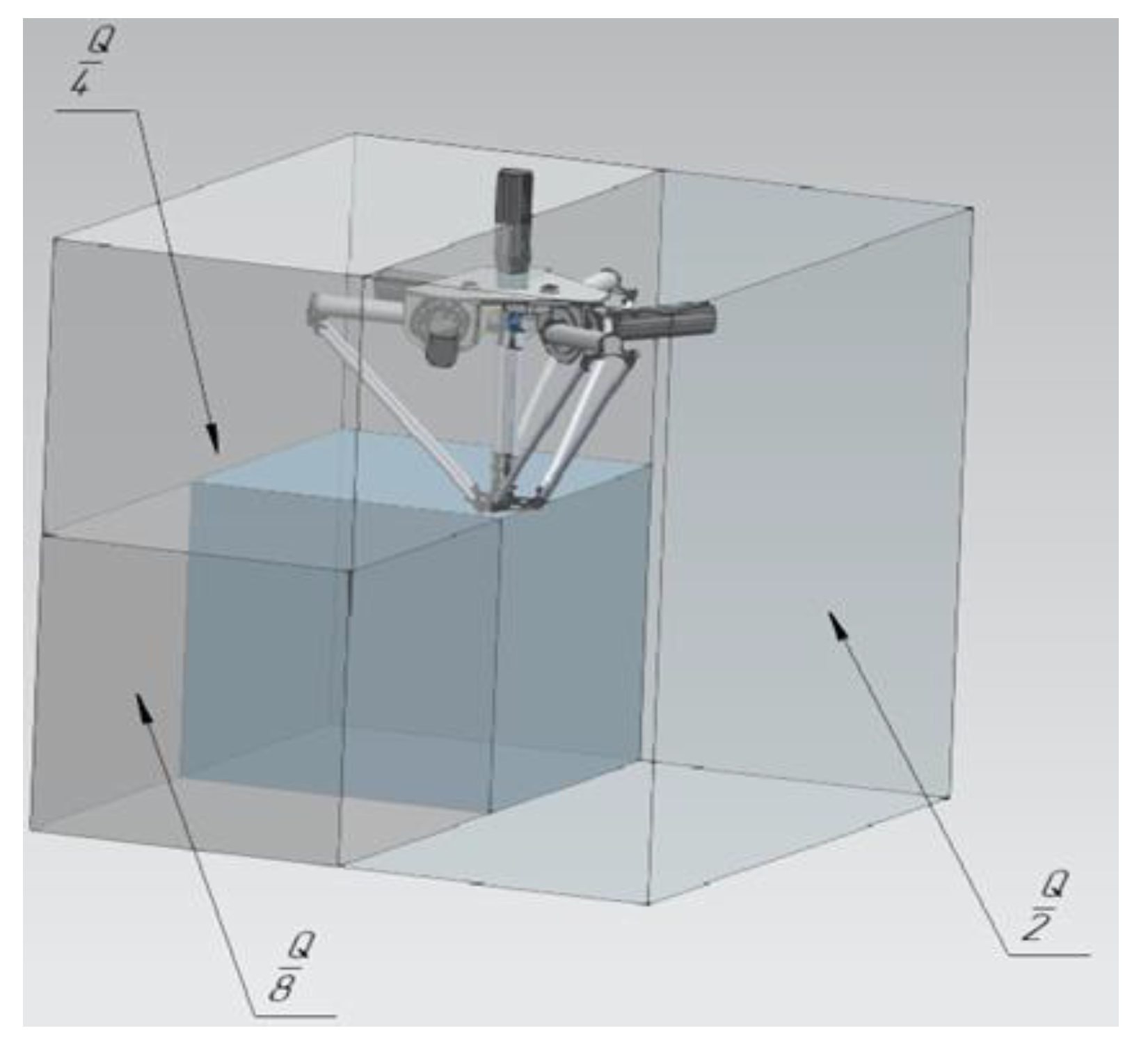
The algorithm works with a system of inequalities written in a general form:

$$\{\begin{array}{c}\begin{array}{c}{g}_1\left(x\right)\le 0,\\ \dots \end{array}\\ \begin{array}{c}{g}_m\left(x\right)\le 0\\ a_i\le x_i\le b_i, i=1,\dots ,n.\end{array}\end{array}$$

(12)

The initial box Q, which includes the entire set of solutions X, is determined by the constraints of the intervals $a_i\le x_i\le b_i, i=1,\dots ,n$. Consider an arbitrary box B. Let m $m\left(B\right)=\underset{i=1,\dots ,m}{\max } \underset{x\in B}{\min } g_i\left(x\right)$ and $M\left(B\right)=\underset{i=1,\dots ,m}{\max } \underset{x\in B}{\max } g_i\left(x\right)$. If $m\left(B\right)>0,$ then B contains no possible points for system (12). The proposed algorithm excludes such boxes. If $M \left(B\right) \le 0$, then each point of the box is a possible solution. Therefore, it can be added to the coverage as an inner box. If a box cannot be excluded, it is divided into two smaller boxes if its diameter is not less than the specified precision δ. (Figure 6). The check is iteratively repeated for boxes formed after division until their size becomes less than precision δ.

The algorithm for determining the workspace, taking into account singularity zones, is similar and differs in a large number of inequalities in the system, as well as additional conditions when checking m (B) and M (B), taking into account the strict inequality for the determinant of the Jacobian matrix.

Equation (11) is used instead of the system of inequalities in the algorithm for determining the singularity zones. To find the set of its solutions, we calculate M (B), which is calculated as $M\left(B\right)=\underset{i\in 1,k}{\min } \underset{x\in B}{\max } g_j\left(x\right)$, the condition for adding is that there is no inner coverage, and the condition for excluding boxes will take the form:

$$M\left(B\right)<0 \mathrm{V} m\left(B\right)>0$$

(13)

We use synthesized algorithms for numerical simulation. A program was written in the C++ programming language to implement the developed algorithms.

4. Simulation Results of Workspace Taking into Account Singularity Zones

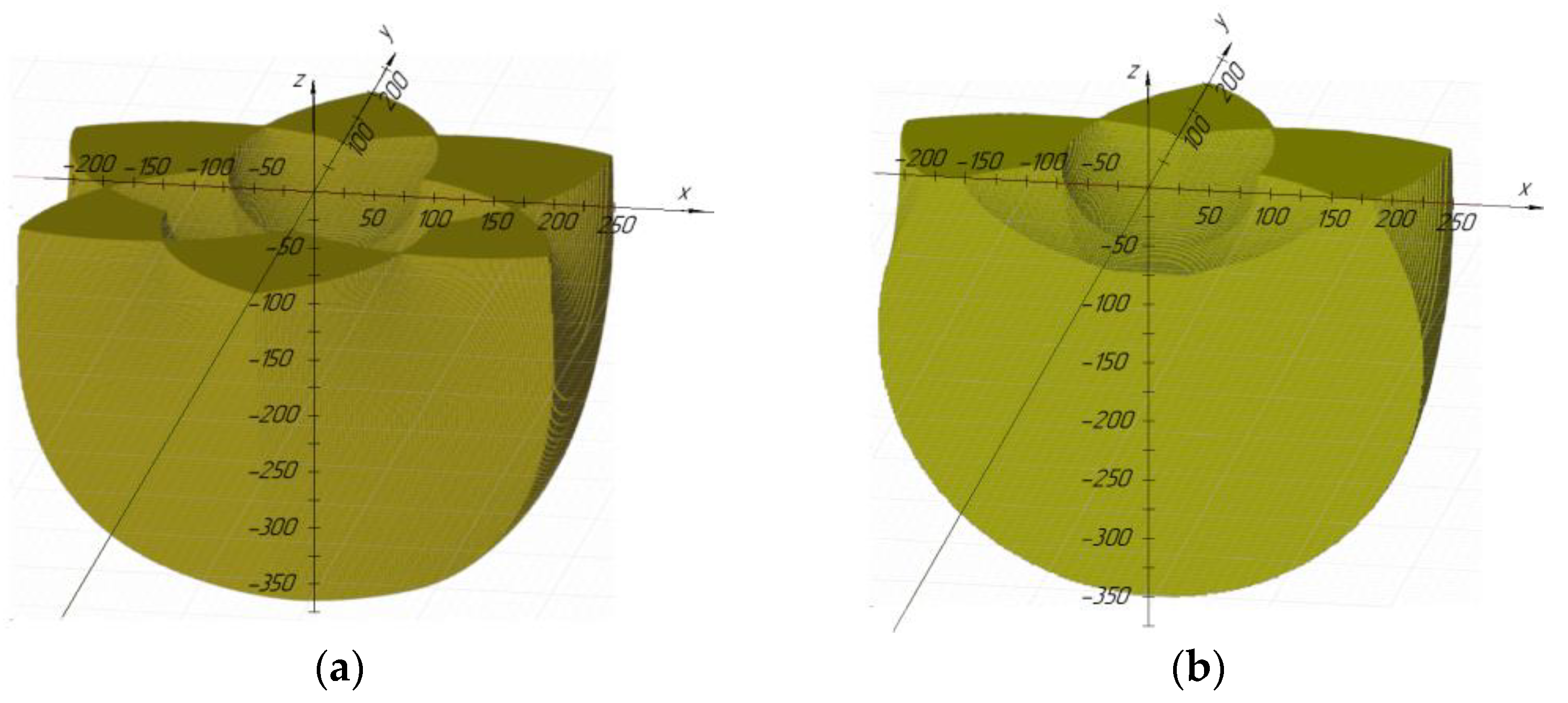
The results of modeling the workspace were obtained for the following parameters of the DeLi manipulator: a = 450 mm, c = 200 mm, d = 150 mm, e = 230 mm. The visualization of the results of modeling the workspace is carried out by converting the covering set describing the workspace into a universal format of 3D models—an STL file. The constructed workspace without taking into account singularity zones is shown in Figure 7. Figure 7a shows the workspace in full, 7b—in section by the XOZ plane. In order to increase the performance, the processor multithreading is applied using the OpenMP package. The computation time for the approximation accuracy δ = 2 mm and the grid dimension for performing computations of the 32 × 32 × 32 functions was 67 s for each inverse kinematics case.

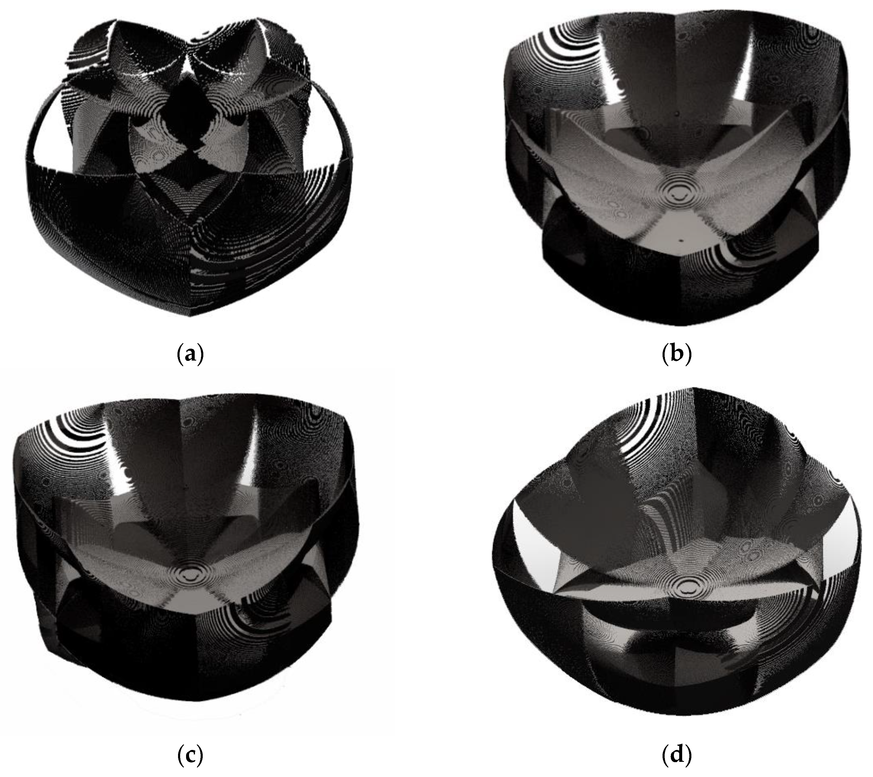
The results of modeling the workspace taking into account singularity zones are shown in Figure 8. Figure 8a shows the regions corresponding to the singularity zones when using the “+” sign in inverse kinematics (2), Figure 8b—when using the “−” sign, Figure 8c—with all eight possible combinations of the “+” and “−” signs in the inverse kinematics, Figure 8d—for all combinations within the workspace. The average computation time for an approximation accuracy δ = 2 mm and a grid dimension of 64 × 64 × 64 on a personal computer was 32 s.

The simulation results show the following conclusions. The inner part of the workspace has a positive sign of the determinant of the Jacobi matrix if two or three kinematic chains have a “−” sign in the inverse kinematics. The negative sign of the determinant is obtained in the opposite cases, that is, if the “+” sign is selected for at least two chains. With this in mind, when determining the workspace, taking into account singularity zones for four possible solutions, we add the condition of the positive determinant, i.e., det (J_A) > 0, and for the other four, the condition of negativity, i.e., det (J_A) < 0.

Table 1. Volumes of workspaces taking into account singularity zones.

Configuration No.	Sign in Inverse Kinematics			Sign of the Jacobi Determinant	Volume of the Workspace, ×104 mm3		Volume Reduction in%
	${\mathbf{\theta }}_1$	${\mathbf{\theta }}_2$	${\mathbf{\theta }}_3$		With Singularity Zones	Without Singularity Zones
1	−	−	−	−	5140	4822	6.18
2	−	−	+	−	5034	4285	14.88
3	−	+	−	−	5034	4285	14.88
4	−	+	+	+	4931	4705	4.58
5	+	−	−	−	5034	4285	14.88
6	+	−	+	+	4931	4705	4.58
7	+	+	−	+	4931	4705	4.58
8	+	+	+	+	4831	4449	7.91

shows the simulation results for these cases.

As can be seen from the table, out of eight options for the inverse kinematics, four groups of solutions can be distinguished: 1—all kinematic chains with “+”, 2—all with “−”, 3—one chain with “+” and two with “−”, and also 4—two with “+” and one with “−”. The first two groups correspond to one option, the second two to three options each. Considering the symmetry of the robot structure, the volume of the resulting workspace is practically the same for all variants of the group. This is confirmed by the calculated values of the volume of the workspace. The table also shows that options 2, 3, and 5, as well as 4, 6, and 7 correspond to the same volume of the workspace. Figure 9 shows the workspaces corresponding to each of the groups.

In Figure 10, it can be seen that taking into account the singularity zones led to a decrease in the size of the workspace by 4.58–14.88%, depending on the combination of possible solutions to the inverse kinematics. In addition to singularity zones, the shape and volume of the workspace are directly influenced by the interferences of the robot links with the platforms and with each other.

5. Determination of the Interference of the Links of the Mechanism

The interferences of the links of the mechanism can be divided into three groups:

-

Interference at small angles between links connected by joints.

-

The interference of links with platforms.

-

The interference of links that are not connected to each other.

The first group can be determined, taking into account the restrictions on the angles of rotation in the joints $B_i$ and $C_i$ (Figure 10):

$$\left\{\begin{array}{c}{\alpha }_i\in \left[{\alpha }_{\min };{\alpha }_{\max }\right]\\ {\beta }_i\in \left[{\beta }_{\min };{\beta }_{\max }\right]\\ {\gamma }_i^{\left(j\right)}\in \left[{\gamma }_{\min };{\gamma }_{\max }\right]\end{array}\right\}$$

(14)

The angles can be determined using the formula for the cosines between vectors:

$${\alpha }_i=\frac{\left(x_{Ai}-x_{Bi}\right)\left(x_{Ci}-x_{Bi}\right)+\left(y_{Ai}-y_{Bi}\right)\left(y_{Ci}-y_{Bi}\right)+\left(z_{Ai}-z_{Bi}\right)\left(z_{Ci}-z_{Bi}\right)}{de}$$

(15)

$${\beta }_i=\frac{\sqrt{3}\left(\left(x_{Bi}-x_{Ci}\right)\left(x_P-x_{Ci}\right)+\left(y_{Bi}-y_{Ci}\right)\left(y_P-y_{Ci}\right)+\left(z_{Bi}-z_{Ci}\right)\left(z_P-z_{Ci}\right)\right)}{ce}$$

(16)

$${\gamma }_i^{\left(Bi1\right)}=\frac{\left(x_{Ci1}-x_{Bi1}\right)\left(x_{Bi2}-x_{Bi1}\right)+\left(y_{Ci1}-y_{Bi1}\right)\left(y_{Bi2}-y_{Bi1}\right)+\left(z_{Ci1}-z_{Bi1}\right)\left(z_{Bi2}-z_{Bi1}\right)}{he}$$

(17)

$${\gamma }_i^{\left(Bi2\right)}={\gamma }_i^{\left(Ci1\right)}=-{\gamma }_i^{\left(Ci2\right)}=-{\gamma }_i^{\left(Bi1\right)}$$

(18)

where $x_{A1}=z_{A1}=z_{A2}=z_{A3}=x_{B1}=0$,$x_{A2}=\frac{a}{4}$, $x_{A3}=-\frac{a}{4}$, $y_{A1}=-\frac{a}{2\sqrt{3}}$, $y_{A2}=y_{A3}=-\frac{a}{4\sqrt{3}}$, $y_{B1}=y_{A1}-d\cos \left({\theta }_1\right)$, $z_{Bi}=-d\sin \left({\theta }_i\right)$, $x_{B2}=x_{A2}+\frac{\sqrt{3}d\cos \left({\theta }_2\right)}{2}$,$y_{B2}=y_{A2}+\frac{d\cos \left({\theta }_2\right)}{2}$, $x_{B3}=x_{A3}-\frac{\sqrt{3}d\cos \left({\theta }_3\right)}{2}$,$y_{B3}=y_{A3}+\frac{d\cos \left({\theta }_3\right)}{2}$,$z_{Ci}=z_P$, $x_{C1}=x_P$, $y_{C1}=y_P-\frac{c}{\sqrt{3}}$, $x_{C2}=x_P+\frac{c}{2}$, $y_{C2}=y_{C3}=y_P+\frac{c}{2\sqrt{3}}$, $x_{C3}=x_P-\frac{c}{2}$, $x_{B31}=y_{B31}$,$z_{B31}=z_{B32}=z_{B3}$.

The second group of interference includes possible interference of links with platforms $A_1, A_2,A_3$ and $C_1, C_2, C_3$. In this case, the interference with the platform $C_1, C_2, C_3$ is excluded by condition (14). The interference of links $A_i, B_i$ and $B_{i1},B_{i2}$ with platform $A_1, A_2, A_3$ is also excluded by condition (1). Let us add the conditions for the appearance of the remaining interference, namely links $B_{i1}, C_{i1}$ and $B_{i2}, C_{i2}$ with platform $A_1, A_2, A_3$ (Figure 11). The first condition for the occurrence of interference is:

$$z_{Bi}\ge 0$$

(19)

If condition (19) is satisfied for the joint $B_i$, then we calculate the coordinate points of the points $D_{i1}$ and $D_{i2}$, lying on the segments $B_{i1}, C_{i1}$ and $B_{i2}, C_{i2}$, respectively, which can be the interference points of the segments with the platform $A_1, A_2, A_3$:

$$z_{Di1}=z_{Di2}=0$$

(20)

$$x_{Di1}=x_{Bi1}+\frac{-z_{Bi1}\left(x_{Ci1}-x_{Bi1}\right)}{z_{Ci1}-z_{Bi1}}, y_{Di1}=y_{Bi1}+\frac{-z_{Bi1}\left(y_{Ci1}-y_{Bi1}\right)}{z_{Ci1}-z_{Bi1}}$$

(21)

$$x_{Di2}=x_{Bi2}+\frac{-z_{Bi2}\left(x_{Ci2}-x_{Bi2}\right)}{z_{Ci2}-z_{Bi2}}, y_{Di2}=y_{Bi2}+\frac{-z_{Bi2}\left(y_{Ci2}-y_{Bi2}\right)}{z_{Ci2}-z_{Bi2}}$$

(22)

The platform is an equilateral triangle with points $A_1, A_2, A_3$ being the midpoints of the sides. The coordinates of the vertices $A_1^{\prime }, A_2^{\prime }, A_3^{\prime }$ are defined as:

$$z_{A_1^{\prime }}=z_{A_2^{\prime }}=z_{A_3^{\prime }}=x_{A_3^{\prime }}=0, x_{A_1^{\prime }}=-\frac{a}{2}, x_{A_2^{\prime }}=\frac{a}{2}, y_{A_1^{\prime }}=y_{A_2^{\prime }}=-\frac{a}{2\sqrt{3}},$$

(23)

$$y_{A_3^{\prime }}=\frac{a}{\sqrt{3}}$$

(24)

As a result, it is required to check in the two-dimensional plane XOY whether the points $D_{i1}$ and $D_{i2}$ belong to the triangle $A_1^{\prime }{A}_2^{\prime }{A}_3^{\prime }$. If at least one of the points is included in the triangle, then there is interference with the platform.

We define the third group of interference using an approach based on determining the minimum distance between the segments drawn between the centers of the joints of each of the links. In [22,23], a similar condition is used, but the approach has drawbacks. In particular, the authors propose to determine the interference of the segments on the auxiliary plane, and not the distance between the nearest points. This does not allow identifying such an interference of links in which there is no interference of the axes.

The approach proposed in the current work is as follows. We construct an auxiliary plane to determine the interference of the links of the mechanism. This plane is parallel to the axis of one of the links and to which the axis of the other link belongs. In this case, the condition for the absence of interference of the links will take the form:

$$\sqrt{u_1^2+u_2^2}>{\mathrm{r}}_{link1}+{\mathrm{r}}_{link2},$$

(25)

where u₁ is the distance between the axis of a link that does not belong to the plane and the auxiliary plane, u₂ is the distance between the nearest points of the segments connecting the centers of the joints of each of the links when projecting a segment that does not belong to the auxiliary plane onto this plane, and ${\mathrm{r}}_{link1}, {\mathrm{r}}_{link2}$ are the radiuses of the links.

It is worth noting the special case when the links are parallel to each other and the construction of an auxiliary plane is not required.

The algorithm for determining the interference of links is as follows:

• Determine the coordinates of the centers of the joints of each of the links.
• Draw segments 1 and 2 between the centers of the joints at each of the links, respectively.
• If the line segments are parallel to each other, then go to step 5. Otherwise, go to step 9.
• Rotate the line segments relative to the vertex of one of the line segments so that they become parallel to the OX axis.
• Determine the distance $u_1$ between the straight lines passing through the segments.
• Let us project the line segments onto the OX axis.
• Determine the distance $u_2$ between the nearest points of the line segments.
• If condition (25) is satisfied, then there is no interference. Completion of the algorithm.
• Construct an auxiliary plane in which segment 1 will lie, and to which segment 2 will be parallel.
• Determine the distance $u_1$ between line segment 2 and the construction plane.
• Project line segment 2 onto a construction plane.
• Determine the distance $u_2$ between the nearest points of segment 1 and the projection of segment 2.
• If condition (25) is satisfied, then there is no interference. Completion of the algorithm.

A more detailed approach to the definition of the third group of interference is presented in [35].

The proposed approach can be similarly applied to determine the interference between the links of the Uni and DeLi robots. In this case, it is possible to discretely separate the trajectories of the robots in the process of collaborative work of two robots. Then, it is required to determine the positions of the joints for each of the positions of the robots. Using the coordinates of the joints, one must check the intersection of all combinations of links using condition (25) and the above algorithm.

6. Analysis of the Workspace Taking into Account the Interference of the Links

The coverage obtained at the stage of defining the workspace is used to determine the positions of the end-effector inside the workspace, in which the interference of the links occurs. The coverage is divided into many boxes of equal size less than the approximation accuracy.

For the coordinate of the center of each of the boxes, conditions (14) and (25) are checked. If all the conditions are met, it is entered into a new set. The resulting set will contain boxes that correspond to the workspace without interference.

Workspace for configuration 1 according to Table 1 after excluding interference areas, as well as interference areas for a = 450 mm, c = 200 mm, d = 150 mm, e = 230 mm, ${\alpha }_{min}$ = ${\beta }_{min}$= ${\gamma }_{min}$ = 10°, ${\alpha }_{max}$ = ${\beta }_{max}$= ${\gamma }_{max}$ = 350°, ${\mathrm{D}}_{link}$ = 10 mm are shown in Figure 12.

Table 2. Volumes of workspaces taking into account link interference.

Configuration No.	Volume of the Workspace, ×104 mm3		Volume Reduction in%
	With Interference Areas	Without Interference Area
1	4822	2457	49.05
2	4285	1741	59.37
3	4285	1741	59.37
4	4705	1183	74.86
5	4285	1741	59.37
6	4705	1182	74.86
7	4705	1182	74.86
8	4449	806	81.88

shows the change in the volume of the workspace, taking into account the interference, without interference of links, as well as volume reduction for various configurations by taking into account the interference.

As can be seen from Table 2, with an increase in the number of kinematic chains, which corresponds to “+” in the inverse kinematics, the greater the percentage of the workspace that is excluded due to interference. This is due to the fact that in this case the kinematic chains are “bent” inward. As a result, the volume of the workspace for the first configuration is 3.05 times greater than the volume for the eighth configuration.

Visualization of the positions of the links at which they intersect occurs to verify the results of determining the interference. Figure 13 shows some of the link crossings that occur.

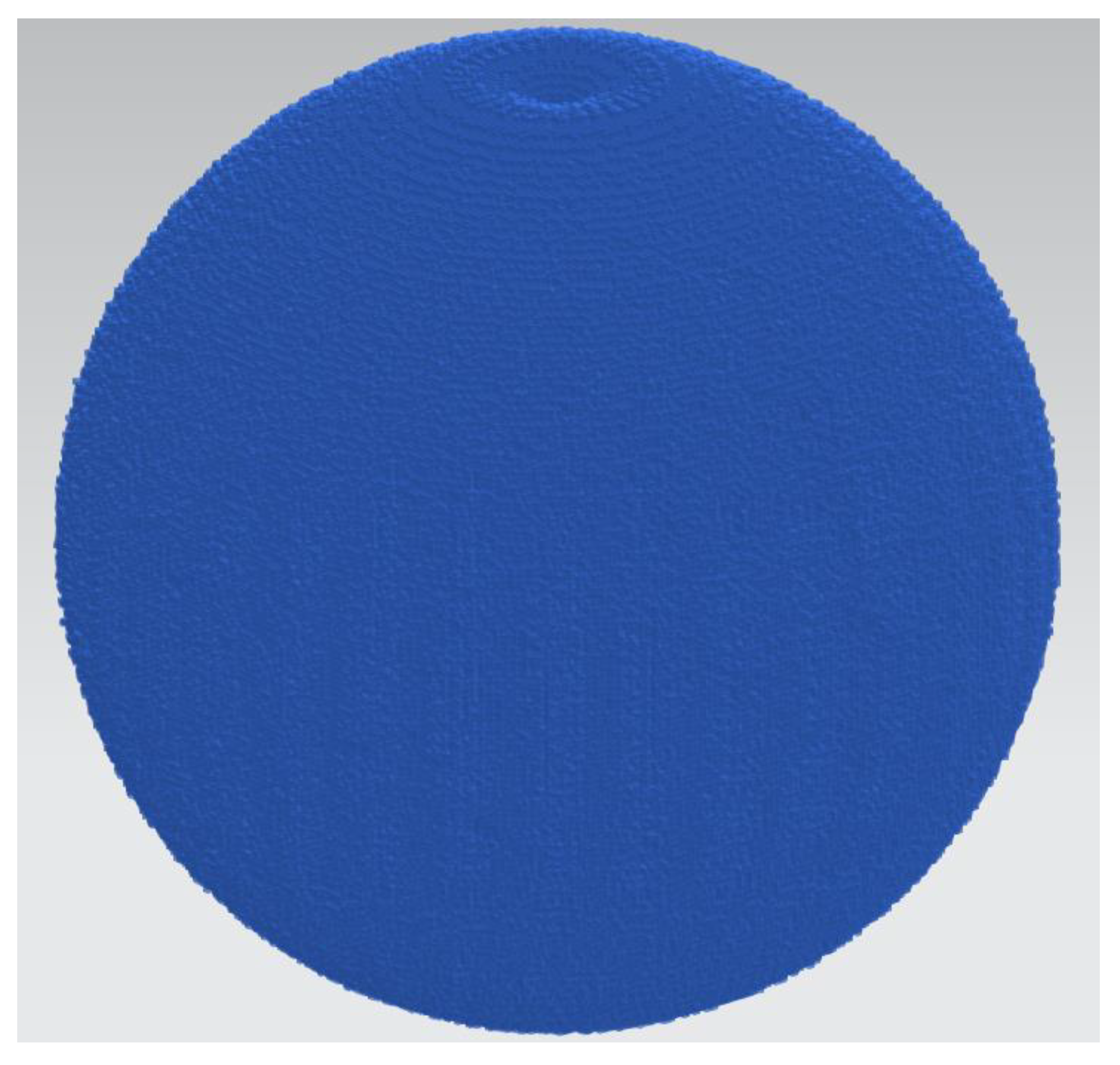
Figure 12 shows that the main inner part of the work area is round. Simulations were also performed for other link sizes (

Table 3. Volumes of workspaces taking into account link interference.

No.	a	c	d	e
1	600	50	1200	1200
2	200	300	400	800
3	700	300	700	700

). The simulation results are shown in Figure 14. As can be seen from the figures, the workspace for various sizes has a round shape.

7. Geometric Parameters Optimization

Next, we will optimize the geometric parameters of the mechanism. The volume of the workspace, taking into account singularity zones and the interference of links, is an optimization criterion. Determination of the optimal sizes of links a, c, d, and e was carried out in several stages. At each stage, the volume of the workspace was calculated taking into account the interference of the links for various combinations of sizes. The ranges of resizing and the iteration step are reduced with each stage to reduce the computational complexity.

Numerical values are given in

Table 4. Stages of determining the optimal link lengths.

Stage	amin	amax	cmin	cmax	dmin	dmax	emin	emax	Step	Required Volume, m3
1	50	1700	50	1700	50	1700	50	1700	100	1.5
2	50	320	50	320	200	800	750	1320	30	2.4
3	51	139	81	169	346	634	1020	1316	8	2708
4	60	72	82	94	469	520	1173	1227	3	27,105
5	61	65	83	87	512	519	1183	1190	1	-

. The last column contains the volume of the workspace, which is a criterion for excluding or including in the next stage a certain part of the size range. Constant dimensions for modeling: h = 100 mm, ${\mathrm{D}}_{link}$ = 30 mm. The sum of the dimensions a, c, d, and e was taken to be constant and equal to 1850 mm. The amount was selected in accordance with the dimensions of the industrial robot ABB IRB 360: a ≈ 600 mm, c ≈ 100 mm, d ≈ 350 mm, e ≈ 100 mm. It should be noted that at the first stage, the computations were carried out for all configurations; however, the condition for the required volume of the workspace was fulfilled only for configurations 1 and 2/3/5. At the second stage, the volume condition was met only for the first configuration. In this regard, modeling was carried out only for the first configuration starting from the third stage.

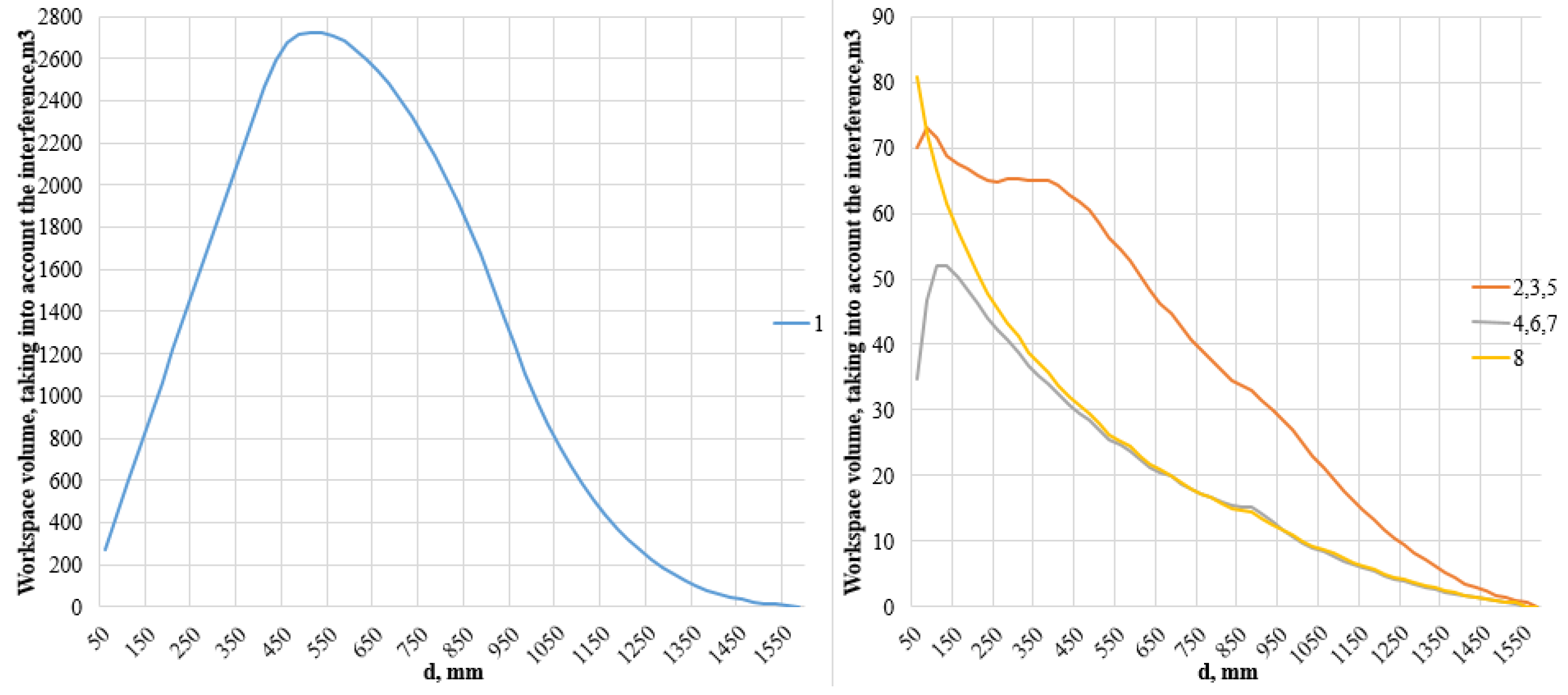
The maximum workspace is reached at a = 61 mm, c = 86 mm, d = 513 mm, and e = 1190 mm. For such a ratio of dimensions, the total volume of the workspace, taking into account singularity zones, is 4.597 m³, of which 2.714 m³ is an area without interference of links. Thus, assuming the conditional size of the side of the base a = 1, the ratios of the sizes c, d, and e were 1.41, 8.41, and 19.51, respectively.

The dependence of the volume of the workspace for various configurations on the change in the parameters d for a = 61 mm and c = 86 mm, e = (1850 − a − c − d) is shown in Figure 15. The numerical values of the workspace volume for the plot are obtained by iterative execution of the developed program for various parameters.

Figure 16 shows the dependence of the proportion of areas in which interference occurs in the total volume of the workspace depending on the parameters d and e. The graphs show that for the first configuration, the fraction of interference decreases with increasing size d. For the rest of the configurations, the percentage of interference for almost all sizes d is more than 90%.

Let us perform the second stage of optimization. It takes into account the requirements of the aliquoting process. The required workspace height $h_c$ is based on the requirements of tube and pipette sizes (350 mm). We can conclude that the manipulator workspace is round based on the previous analysis. Based on this, an optimization problem can be posed, which maximizes the radius $r_c$ of a cylinder of a given height $h_c$, which can be inscribed into the manipulator’s workspace. In this case, the sum of the dimensions $a, c, d,$ and $e$ of the manipulator should also be minimized. Therefore, the general criterion k can be written as:

$$k=\frac{a+c+d+e}{r_c}$$

(26)

The optimization was performed in several stages, similar to the optimization performed above to maximize the workspace. Initial data for optimization: $a\in \left[30;1500\right], c\in \left[30;1500\right], d\in \left[30;1500\right], e\in \left[30;1500\right], h_c=350$ mm. As a result, the optimal value of the criterion $k=1.778$ was obtained for the following dimensions: $a=61$ mm, $c=87$ mm, $d=478$ mm, $e=1485$ mm, $r_c=1187,29$ mm. The simulation of the workspace was performed for the obtained dimensions. Figure 17 shows that the workspace completely includes the cylinder with the calculated radius.

An additional simulation was performed to compare the results of the two optimizations. The volume of the workspace and the maximum cylinder diameter were calculated for both optimal results. The parameters obtained during the first optimization were changed while maintaining the ratio 1:1.41:8.41:19.51. The change is necessary due to the incorrectness of comparing results that have a different sum of parameters. The sum of the parameters for the second optimization was 2111 mm. Therefore, the dimensions of the first optimization were changed so that their sum was 2111 mm. The obtained initial data and simulation results are shown in

Table 5. Stages of determining the optimal link lengths.

Optimization No.	a	c	d	e	Sum	Volume, m3	Cylinder Radius
1	69.606	98.133	585.375	1357.886	2111	4.024	1085.91
2	61	87	478	1485	2111	4.005	1187.29

.

As can be seen from the table, the workspace volume was larger as expected for the parameters obtained as a result of the first optimization and the maximum radius of the inscribed cylinder for the second optimization. However, it should be noted that the workspace volume in the first case turned out to be only 0.47% larger, while the radius for the second case was larger by 9.34%. Therefore, in this case, the radius of the inscribed cylinder is the main criterion for the problem of aliquoting. So, we can conclude that second optimization results should be currently accepted as the final results. However, a formal optimization algorithm will be planned in the future for a further optimization of the obtained results.

The aliquoting process assumes that Uni and DeLi should have a common part of workspaces. The Uni kinematic scheme is shown in Figure 18.

Workspace of Uni is calculated using D-H parameters and transformation matrices, where D-H parameters are equal to $a_2=240$ mm, $a_3=210$ mm, $d_1=150$ mm, $d_4=110$ mm, $d_5=85$ mm, and $d_6=81$ mm. The end-effector positions were calculated in discrete steps using the forward kinematics. The calculated positions were entered into the workspace array. The resulting array was exported to the STL model. Likewise, a program was written in the C++ programming language to implement the developed algorithm. The Uni workspace is shown in Figure 19.

Taking into account the calculated workspace of the Uni robot, we perform a simulation of a robotic system. The workspace models of robots were exported to the CAD system. The relative position of the robots was determined taking into account their workspaces and the requirements for the absence of intersections of links of mechanisms. Simulation of collaborative work of robots is shown in Figure 20. The execution of operations should be consistent: the Uni manipulator delivers a rack with test tubes to the joint workspace; then the DeLi manipulator performs the aliquoting process. The simulation confirmed the absence of intersections during collaborative work.

Figure 21 shows the intersection of the DeLi and Uni workspaces. The intersection area is sufficient to accommodate a rack with 96 test tubes. Based on this, it can be concluded that the workspace of the DeLi robot and the relative position of the robots meet the requirements of the aliquoting process. The above conditions are met if the robot Uni is fixed relative to the coordinate system DeLi at a point with coordinates (0, 830, −897).

8. Conclusions

This article discusses a new robotic system design for aliquoting of biomaterial based on a Delta-type parallel robot with revolute kinematic joints. For the proposed robotic system, effective numerical methods and algorithms for determining the workspace, taking into account singularity zones and interference of links, have been developed and tested. An optimal design procedure has been carried out and robot design solution has been selected that achieves the maximum workspace for a given footprint size. For the selected design solution, the optimal ratio of the lengths of links a, c, d, and e relative to the link length a has been determined as being 1:1.41:8.41:19.51, respectively. The parameters were optimized taking into account the requirements of the aliquoting process. As a result, the optimal value of the criterion $k=1.778$ was obtained for the following dimensions: $a=61$ mm,$c=87$ mm, $d=478$ mm,$e=1485$ mm, and $r_c=1187,29$ mm.