
Solar Irradiance Forecasting Using Dynamic Ensemble Selection

 , , , , , ,
Abstract
:1. Introduction
- Reduces the risk of selecting an inappropriate model;
- Dynamically searches for the most suitable forecaster to predict a given local pattern in a solar irradiance series;
- It is an agnostic model since other forecasting models can be explored in the pool;
- Increases the generalization capacity of the system.
2. Related Works
3. Background
3.1. Autoregressive and Moving Average Model
3.2. Random Forest
3.3. Gradient Boosting
3.4. Support Vector Regression
3.5. Multilayer Perceptron
3.6. Extreme Learning Machines
3.7. Deep Belief Network
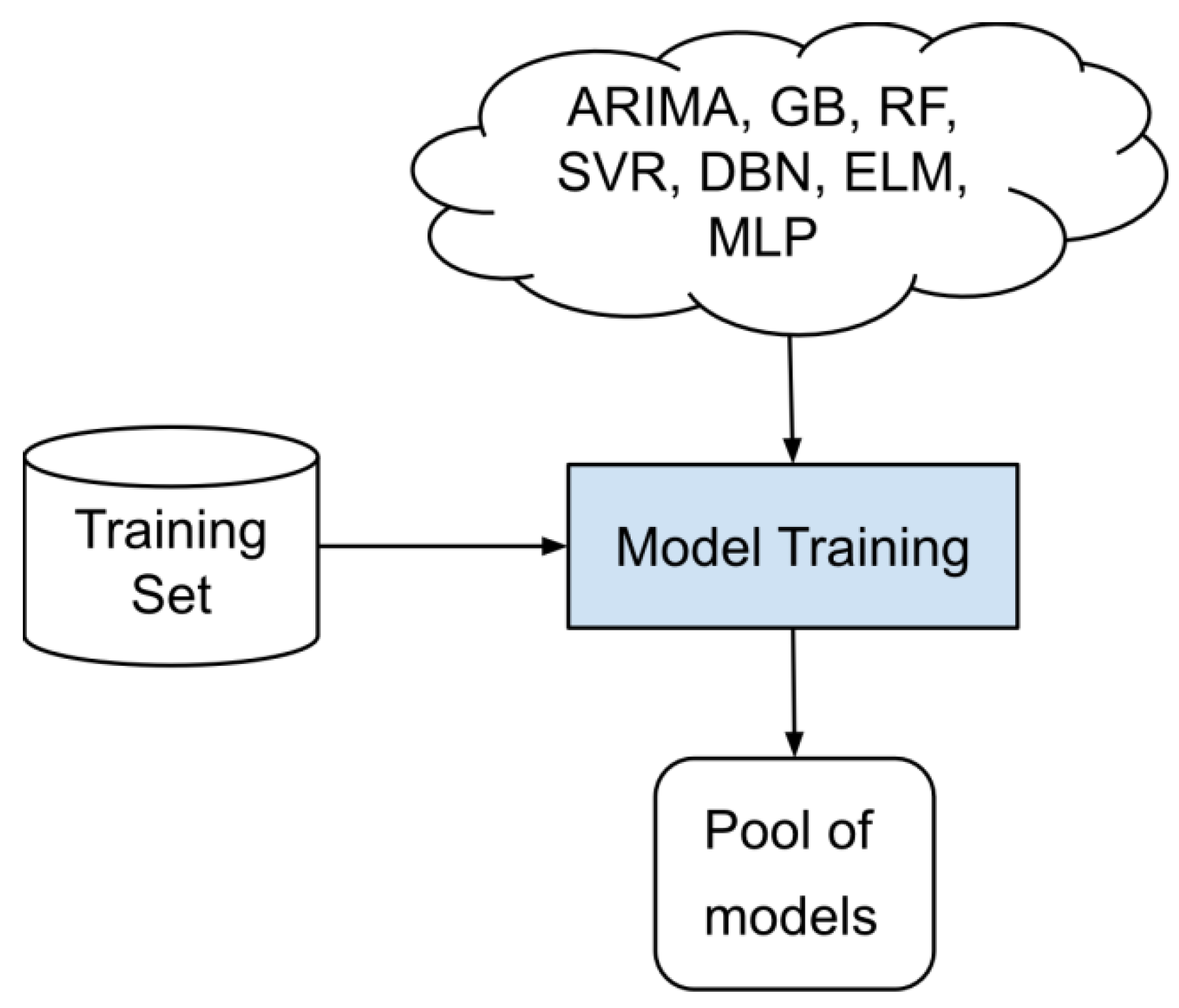
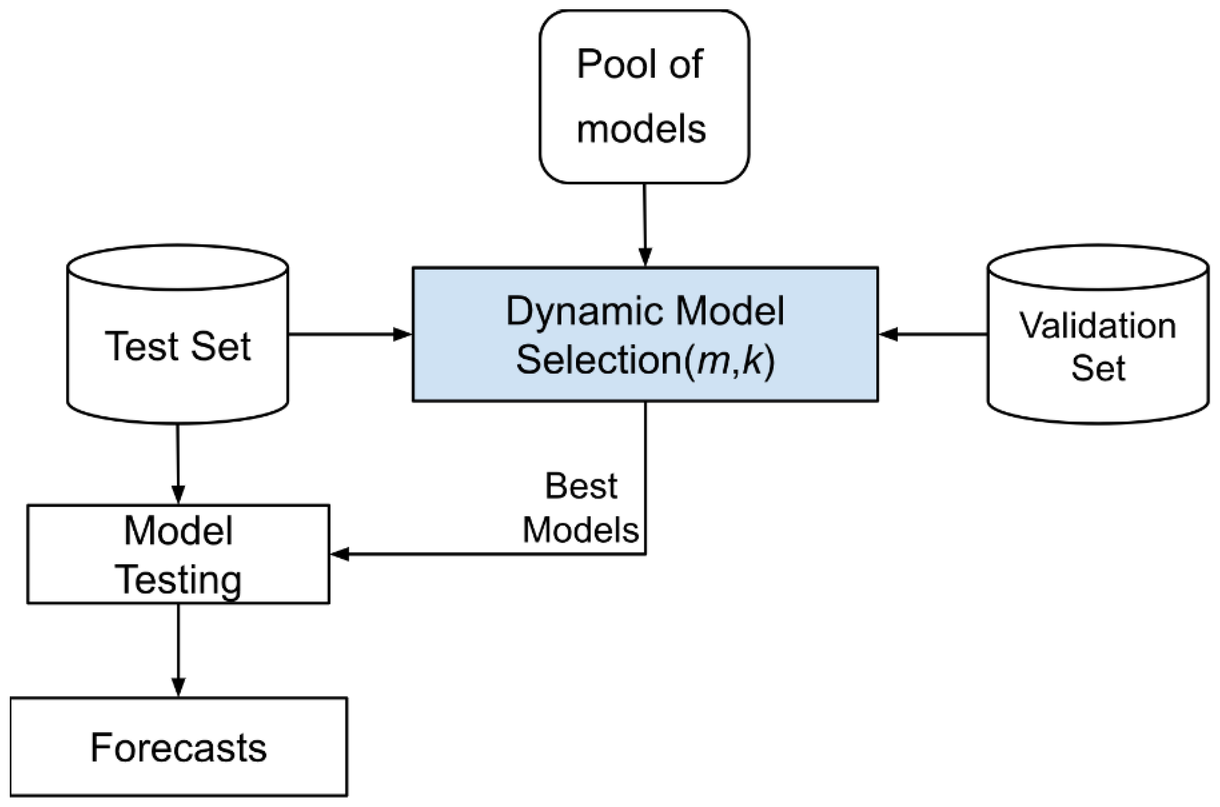
4. Proposed Method
5. Experiments
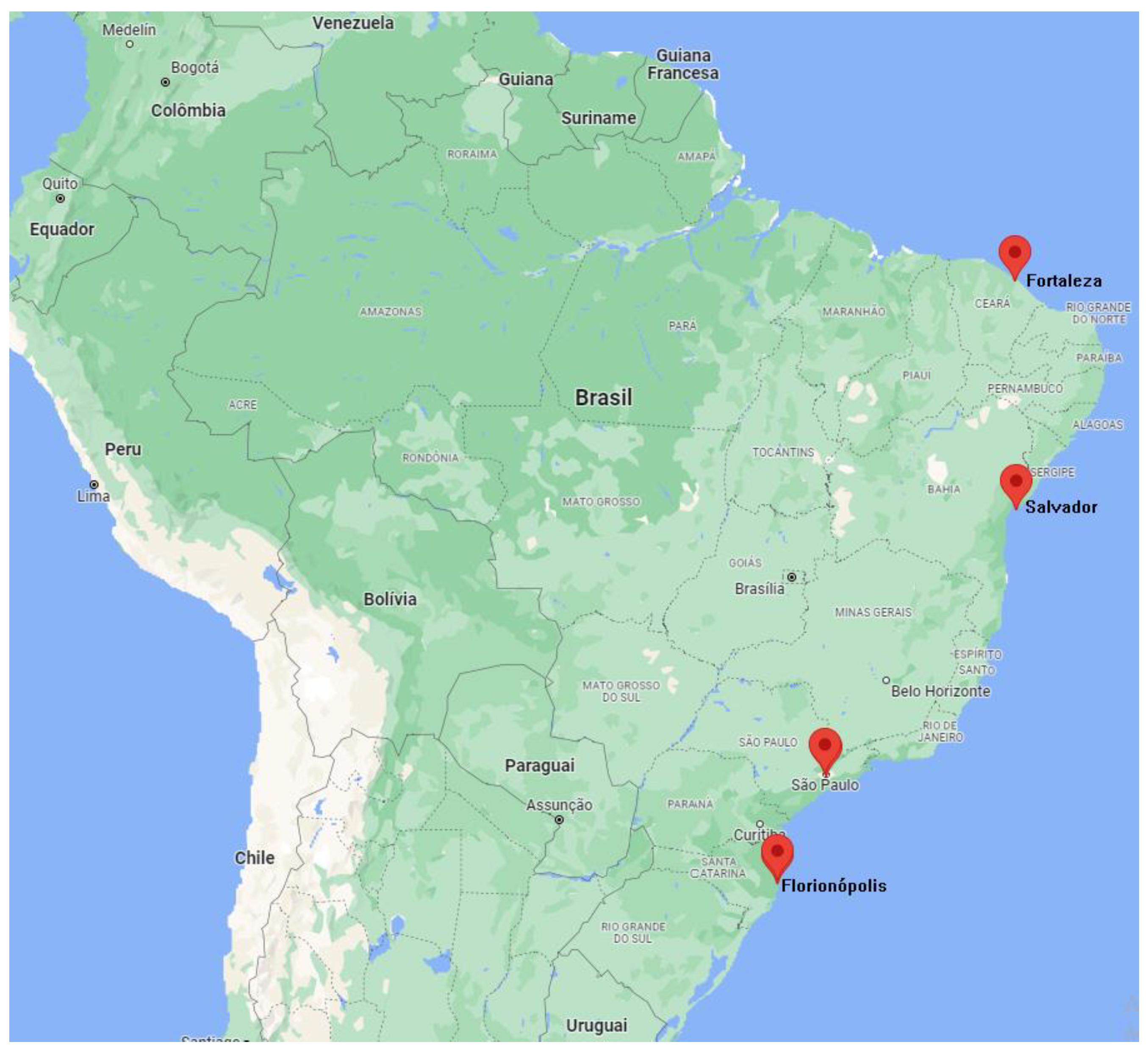
5.1. Data Description
5.2. Evaluation Metrics
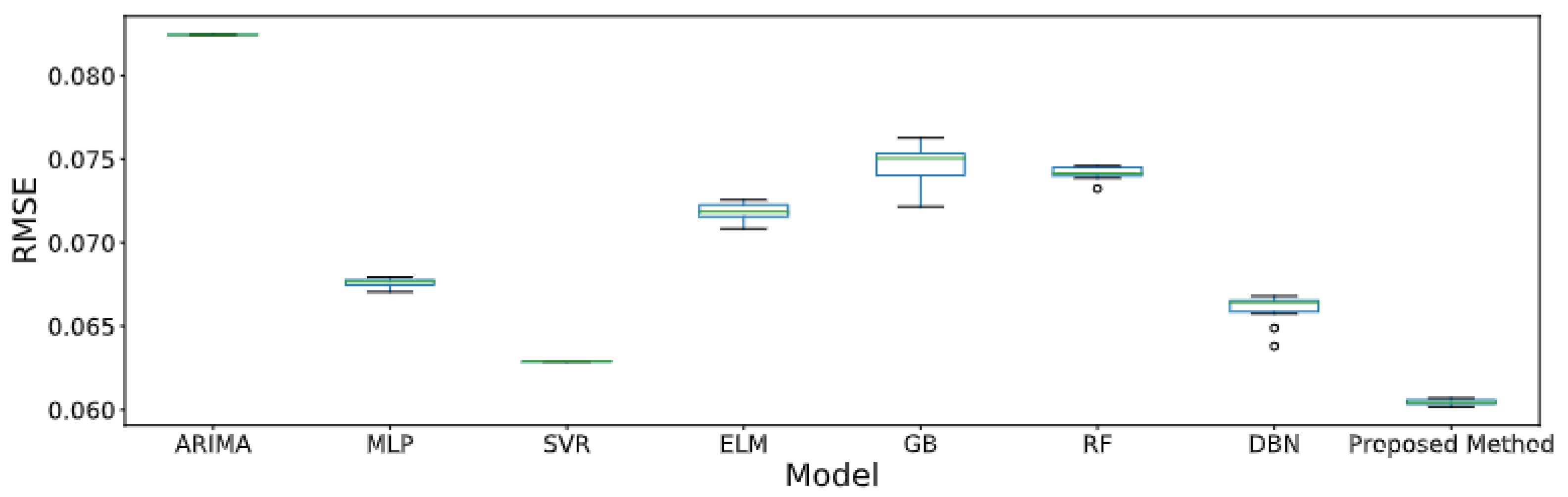
5.3. Results
5.4. Discussion
6. Conclusions
Author Contributions
Funding
Institutional Review Board Statement
Informed Consent Statement
Data Availability Statement
Acknowledgments
Conflicts of Interest
References
- Khan, A.M.; Osińska, M. How to predict energy consumption in BRICS countries? Energies 2021, 14, 2749. [Google Scholar] [CrossRef]
- Jackson, R.B.; Friedlingstein, P.; Andrew, R.M.; Canadell, J.G.; Quéré, C.L.; Peters, G.P. Persistent fossil fuel growth threatens the Paris Agreement and planetary health. Environ. Res. Lett. 2019, 14, 121001. [Google Scholar] [CrossRef] [Green Version]
- Eyring, V.; Gillett, N.; Rao, K.A.; Barimalala, R.; Parrillo, M.B.; Bellouin, N.; Cassou, C.; Durack, P.; Kosaka, Y.; McGregor, S.; et al. Human Influence on the Climate System. In Climate Change 2021: The Physical Science Basis. Contribution of Working Group I to the Sixth Assessment Report of the Intergovernmental Panel on Climate Change; Cambridge University Press: Cambridge, UK, 2021; (in press). [Google Scholar]
- Kumari, P.; Toshniwal, D. Deep learning models for solar irradiance forecasting: A comprehensive review. J. Clean. 2021, 318, 128566. [Google Scholar] [CrossRef]
- Voyant, C.; Notton, G.; Kalogirou, S.; Nivet, M.L.; Paoli, C.; Motte, F.; Fouilloy, A. Machine learning methods for solar radiation forecasting: A review. Renew. Energy 2017, 105, 569–582. [Google Scholar] [CrossRef]
- Espinar, B.; Aznarte, J.L.; Girard, R.; Moussa, A.M.; Kariniotakis, G. Photovoltaic Forecasting: A state of the art. In Proceedings of the 5th European PV-Hybrid and Mini-Grid Conference, Tarragona, Spain, 29–30 April 2010; OTTI-Ostbayerisches Technologie-Transfer-Institut: Tarragona, Spain, 2010; p. 250. [Google Scholar]
- Perera, K.S.; Aung, Z.; Woon, W.L. Machine Learning Techniques for Supporting Renewable Energy Generation and Integration: A Survey. In Proceedings of the Second International Conference on Data Analytics for Renewable Energy Integration, DARE’14, Nancy, France, 19 September 2014; pp. 81–96. [Google Scholar] [CrossRef]
- Frías-Paredes, L.; Mallor, F.; Gastón-Romeo, M.; León, T. Assessing energy forecasting inaccuracy by simultaneously considering temporal and absolute errors. Energy Convers. Manag. 2017, 142, 533–546. [Google Scholar] [CrossRef]
- Moreno-Munoz, A.; de la Rosa, J.J.G.; Posadillo, R.; Bellido, F. Very short term forecasting of solar radiation. In Proceedings of the 2008 33rd IEEE Photovoltaic Specialists Conference, San Diego, CA, USA, 11–16 May 2008; pp. 1–5. [Google Scholar] [CrossRef]
- Diagne, H.M.; Lauret, P.; David, M. Solar irradiation forecasting: State-of-the-art and proposition for future developments for small-scale insular grids. In Proceedings of the WREF 2012-World Renewable Energy Forum, Denver, CO, USA, 13-17 May 2012. [Google Scholar]
- Box, G.E.; Jenkins, G.M.; Reinsel, G.C.; Ljung, G.M. Time Series Analysis: Forecasting and Control; John Wiley & Sons: Hoboken, NJ, USA, 2015. [Google Scholar]
- Zhang, G.P. Time series forecasting using a hybrid ARIMA and neural network model. Neurocomputing 2003, 50, 159–175. [Google Scholar] [CrossRef]
- Guermoui, M.; Melgani, F.; Gairaa, K.; Mekhalfi, M.L. A comprehensive review of hybrid models for solar radiation forecasting. J. Clean. Prod. 2020, 258, 120357. [Google Scholar] [CrossRef]
- de Oliveira, J.F.L.; Silva, E.G.; de Mattos Neto, P.S.G. A Hybrid System Based on Dynamic Selection for Time Series Forecasting. IEEE Trans. Neural Netw. Learn. Syst. 2021, 1–13. [Google Scholar] [CrossRef] [PubMed]
- Izidio, D.M.; de Mattos Neto, P.S.; Barbosa, L.; de Oliveira, J.F.; Marinho, M.H.d.N.; Rissi, G.F. Evolutionary Hybrid System for Energy Consumption Forecasting for Smart Meters. Energies 2021, 14, 1794. [Google Scholar] [CrossRef]
- Campos, D.S.; de Souza Tadano, Y.; Alves, T.A.; Siqueira, H.V.; de Nóbrega Marinho, M.H. Unorganized machines and linear multivariate regression model applied to atmospheric pollutant forecasting. Acta Sci. Technol. 2020, 42, e48203. [Google Scholar] [CrossRef]
- Geman, S.; Bienenstock, E.; Doursat, R. Neural networks and the bias/variance dilemma. Neural Comput. 1992, 4, 1–58. [Google Scholar] [CrossRef]
- Mendes-Moreira, J.; Soares, C.; Jorge, A.M.; Sousa, J.F.D. Ensemble approaches for regression: A survey. ACM Comput. Surv. (Csur) 2012, 45, 1–40. [Google Scholar] [CrossRef]
- Ren, Y.; Zhang, L.; Suganthan, P.N. Ensemble classification and regression-recent developments, applications and future directions. IEEE Comput. Intell. Mag. 2016, 11, 41–53. [Google Scholar] [CrossRef]
- Brown, G.; Wyatt, J.L.; Tino, P.; Bengio, Y. Managing diversity in regression ensembles. J. Mach. Learn. Res. 2005, 6, 41–53. [Google Scholar]
- Webb, G.; Zheng, Z. Multistrategy ensemble learning: Reducing error by combining ensemble learning techniques. IEEE Trans. Knowl. Data Eng. 2004, 16, 980–991. [Google Scholar] [CrossRef] [Green Version]
- Jiang, H.; Dong, Y.; Xiao, L. A multi-stage intelligent approach based on an ensemble of two-way interaction model for forecasting the global horizontal radiation of India. Energy Convers. Manag. 2017, 137, 142–154. [Google Scholar] [CrossRef]
- Jovanovic, R.; Pomares, L.M.; Mohieldeen, Y.E.; Perez-Astudillo, D.; Bachour, D. An evolutionary method for creating ensembles with adaptive size neural networks for predicting hourly solar irradiance. In Proceedings of the 2017 International Joint Conference on Neural Networks (IJCNN), Anchorage, AK, USA, 14–19 May 2017; pp. 1962–1967. [Google Scholar]
- Sun, S.; Wang, S.; Zhang, G.; Zheng, J. A decomposition-clustering-ensemble learning approach for solar radiation forecasting. Sol. Energy 2018, 163, 189–199. [Google Scholar] [CrossRef]
- Rodríguez, F.; Martín, F.; Fontán, L.; Galarza, A. Ensemble of machine learning and spatiotemporal parameters to forecast very short-term solar irradiation to compute photovoltaic generators’ output power. Energy 2021, 229, 120647. [Google Scholar] [CrossRef]
- Demšar, J. Statistical comparisons of classifiers over multiple data sets. J. Mach. Learn. Res. 2006, 7, 1–30. [Google Scholar]
- Zhou, Y.; Liu, Y.; Wang, D.; Liu, X.; Wang, Y. A review on global solar radiation prediction with machine learning models in a comprehensive perspective. Energy Convers. Manag. 2021, 235, 113960. [Google Scholar] [CrossRef]
- Rajagukguk, R.A.; Ramadhan, R.A.; Lee, H.J. A review on deep learning models for forecasting time series data of solar irradiance and photovoltaic power. Energies 2020, 13, 6623. [Google Scholar] [CrossRef]
- Akhter, M.N.; Mekhilef, S.; Mokhlis, H.; Shah, N.M. Review on forecasting of photovoltaic power generation based on machine learning and metaheuristic techniques. IET Renew. Power Gener. 2019, 13, 1009–1023. [Google Scholar] [CrossRef] [Green Version]
- Rigollier, C.; Lefèvre, M.; Wald, L. The method Heliosat-2 for deriving shortwave solar radiation from satellite images. Sol. Energy 2004, 77, 159–169. [Google Scholar] [CrossRef] [Green Version]
- Jiang, Y. Computation of monthly mean daily global solar radiation in China using artificial neural networks and comparison with other empirical models. Energy 2009, 34, 1276–1283. [Google Scholar] [CrossRef]
- Shadab, A.; Said, S.; Ahmad, S. Box–Jenkins multiplicative ARIMA modeling for prediction of solar radiation: A case study. Int. J. Energy Water Resour. 2019, 3, 305–318. [Google Scholar] [CrossRef]
- Voyant, C.; Muselli, M.; Paoli, C.; Nivet, M.L. Numerical weather prediction (NWP) and hybrid ARMA/ANN model to predict global radiation. Energy 2012, 39, 341–355. [Google Scholar] [CrossRef] [Green Version]
- Chen, J.L.; Li, G.S. Evaluation of support vector machine for estimation of solar radiation from measured meteorological variables. Theor. Appl. Climatol. 2014, 115, 627–638. [Google Scholar] [CrossRef]
- Bendiek, P.; Taha, A.; Abbasi, Q.H.; Barakat, B. Solar irradiance forecasting using a data-driven algorithm and contextual optimization. Appl. Sci. 2021, 12, 134. [Google Scholar] [CrossRef]
- Huang, J.; Troccoli, A.; Coppin, P. An analytical comparison of four approaches to modelling the daily variability of solar irradiance using meteorological records. Renew. Energy 2014, 72, 195–202. [Google Scholar] [CrossRef]
- Park, J.; Moon, J.; Jung, S.; Hwang, E. Multistep-ahead solar radiation forecasting scheme based on the light gradient boosting machine: A case study of Jeju Island. Remote Sens. 2020, 12, 2271. [Google Scholar] [CrossRef]
- Fan, J.; Wang, X.; Wu, L.; Zhou, H.; Zhang, F.; Yu, X.; Lu, X.; Xiang, Y. Comparison of support vector machine and extreme gradient boosting for predicting daily global solar radiation using temperature and precipitation in humid subtropical climates: A case study in China. Energy Convers. Manag. 2018, 164, 102–111. [Google Scholar] [CrossRef]
- Elminir, H.K.; Areed, F.F.; Elsayed, T.S. Estimation of solar radiation components incident on Helwan site using neural networks. Sol. Energy 2005, 79, 270–279. [Google Scholar] [CrossRef]
- Salcedo-Sanz, S.; Jiménez-Fernández, S.; Aybar-Ruíz, A.; Casanova-Mateo, C.; Sanz-Justo, J.; García-Herrera, R. A CRO-species optimization scheme for robust global solar radiation statistical downscaling. Renew. Energy 2017, 111, 63–76. [Google Scholar] [CrossRef]
- Salcedo-Sanz, S.; Deo, R.C.; Cornejo-Bueno, L.; Camacho-Gómez, C.; Ghimire, S. An efficient neuro-evolutionary hybrid modelling mechanism for the estimation of daily global solar radiation in the Sunshine State of Australia. Appl. Energy 2018, 209, 79–94. [Google Scholar] [CrossRef]
- Ghimire, S.; Deo, R.C.; Raj, N.; Mi, J. Deep learning neural networks trained with MODIS satellite-derived predictors for long-term global solar radiation prediction. Energies 2019, 12, 2407. [Google Scholar] [CrossRef] [Green Version]
- Zang, H.; Cheng, L.; Ding, T.; Cheung, K.W.; Wang, M.; Wei, Z.; Sun, G. Application of functional deep belief network for estimating daily global solar radiation: A case study in China. Energy 2020, 191, 116502. [Google Scholar] [CrossRef]
- Siqueira, H.; Luna, I.; Alves, T.A.; de Souza Tadano, Y. The direct connection between box & Jenkins methodology and adaptive filtering theory. Math. Eng. Sci. Aerosp. (MESA) 2019, 10. Available online: http://nonlinearstudies.com/index.php/mesa/article/view/1868 (accessed on 5 March 2022).
- de Mattos Neto, P.S.; Ferreira, T.A.; Lima, A.R.; Vasconcelos, G.C.; Cavalcanti, G.D. A perturbative approach for enhancing the performance of time series forecasting. Neural Netw. 2017, 88, 114–124. [Google Scholar] [CrossRef]
- Breiman, L. Random forests. Mach. Learn. 2001, 45, 5–32. [Google Scholar] [CrossRef] [Green Version]
- Ho, T.K. Random decision forests. In Proceedings of the 3rd International Conference on Document Analysis and Recognition, Montreal, QC, Canada, 14–16 August 1995; Volume 1, pp. 278–282. [Google Scholar]
- Amit, Y.; Geman, D. Shape quantization and recognition with randomized trees. Neural Comput. 1997, 9, 1545–1588. [Google Scholar] [CrossRef] [Green Version]
- Cutler, A.; Cutler, D.R.; Stevens, J.R. Random Forests. In Ensemble Machine Learning; Springer: Berlin/Heidelberg, Germany, 2012; pp. 157–175. [Google Scholar]
- Freund, Y.; Schapire, R.E. A decision-theoretic generalization of on-line learning and an application to boosting. J. Comput. Syst. Sci. 1997, 55, 119–139. [Google Scholar] [CrossRef] [Green Version]
- Friedman, J.H. Greedy function approximation: A gradient boosting machine. Ann. Stat. 2001, 29, 1189–1232. [Google Scholar] [CrossRef]
- Kuhn, M.; Johnson, K. Applied Predictive Modeling; Springer: Berlin/Heidelberg, Germany, 2013; Volume 26. [Google Scholar]
- Chen, T.; Guestrin, C. Xgboost: A scalable tree boosting system. In Proceedings of the 22nd ACM Sigkdd International Conference on Knowledge Discovery and Data Mining, San Francisco, CA, USA, 13—17 August 2016; pp. 785–794. [Google Scholar]
- Vapnik, V. The Nature of Statistical Learning Theory; Springer Science & Business Media: Berlin/Heidelberg, Germany, 2013. [Google Scholar]
- de Mattos Neto, P.S.; de Oliveira, J.F.; Domingos, S.d.O.; Siqueira, H.V.; Marinho, M.H.; Madeiro, F. An adaptive hybrid system using deep learning for wind speed forecasting. Inf. Sci. 2021, 581, 495–514. [Google Scholar] [CrossRef]
- Belotti, J.; Siqueira, H.; Araujo, L.; Stevan, S.L.; de Mattos Neto, P.S.; Marinho, M.H.; de Oliveira, J.F.L.; Usberti, F.; Leone Filho, M.d.A.; Converti, A.; et al. Neural-Based ensembles and unorganized machines to predict streamflow series from hydroelectric plants. Energies 2020, 13, 4769. [Google Scholar] [CrossRef]
- Siqueira, H.; Luna, I. Performance comparison of feedforward neural networks applied to stream flow series forecasting. Math. Eng. Sci. Aerosp. (MESA) 2019, 10, 41–53. [Google Scholar]
- Ribeiro, V.H.A.; Reynoso-Meza, G.; Siqueira, H.V. Multi-objective ensembles of echo state networks and extreme learning machines for streamflow series forecasting. Eng. Appl. Artif. Intell. 2020, 95, 103910. [Google Scholar] [CrossRef]
- Huang, G.B.; Zhu, Q.Y.; Siew, C.K. Extreme learning machine: Theory and applications. Neurocomputing 2006, 70, 489–501. [Google Scholar] [CrossRef]
- de Souza Tadano, Y.; Siqueira, H.V.; Alves, T.A. Unorganized machines to predict hospital admissions for respiratory diseases. In Proceedings of the 2016 IEEE Latin American Conference on Computational Intelligence (LA-CCI), Cartagena, Colombia, 2–4 November 2016; pp. 1–6. [Google Scholar]
- Hinton, G.E.; Osindero, S.; Teh, Y.W. A fast learning algorithm for deep belief nets. Neural Comput. 2006, 18, 1527–1554. [Google Scholar] [CrossRef]
- Yang, B.; Zhu, T.; Cao, P.; Guo, Z.; Zeng, C.; Li, D.; Chen, Y.; Ye, H.; Shao, R.; Shu, H.; et al. Classification and summarization of solar irradiance and power forecasting methods: A thorough review. CSEE J. Power Energy Syst. 2021, 1–19. [Google Scholar] [CrossRef]
- Le Roux, N.; Bengio, Y. Representational power of restricted Boltzmann machines and deep belief networks. Neural Comput. 2008, 20, 1631–1649. [Google Scholar] [CrossRef]
- Kourentzes, N.; Barrow, D.K.; Crone, S.F. Neural network ensemble operators for time series forecasting. Expert Syst. 2014, 41, 4235–4244. [Google Scholar]
- Hyndman, R.; Khandakar, Y. Automatic Time Series Forecasting: The forecast package for R. J. Stat. Softw. Artic. 2008, 27, 1–22. [Google Scholar]
- de Mattos Neto, P.S.; Cavalcanti, G.D.; de O Santos Júnior, D.S.; Silva, E.G. Hybrid systems using residual modeling for sea surface temperature forecasting. Sci. Rep. 2022, 12, 487. [Google Scholar] [CrossRef] [PubMed]
- Rodrigues, A.L.J.; Silva, D.A.; de Mattos Neto, P.S.G.; Ferreira, T.A.E. An experimental study of fitness function and timeseries forecasting using artificial neural networks. In Proceedings of the Genetic and Evolutionary Computation Conference (GECCO 2010), ACM, Portland, OR, USA, 7–11 July 2010; pp. 2015–2018. [Google Scholar]
- de Mattos Neto, P.S.G.; Rodrigues, A.L.J.; Ferreira, T.A.E.; Cavalcanti, G.D. An intelligent perturbative approach for the time series forecasting problem. In Proceedings of the IEEE World Congress on Computational Intelligence (WCCI 2010), Barcelona, Spain, 15–17 July 2010; pp. 1–8. [Google Scholar]
- Bhola, P.; Bhardwaj, S. Solar energy estimation techniques: A review. In Proceedings of the 2016 7th India International Conference on Power Electronics (IICPE), Patiala, India, 17–19 November 2016; pp. 1–5. [Google Scholar]
- Srivastava, R.; Tiwari, A.; Giri, V. Solar radiation forecasting using MARS, CART, M5, and random forest model: A case study for India. Heliyon 2019, 5, e02692. [Google Scholar] [CrossRef] [PubMed] [Green Version]
- Hocaoğlu, F.O. Novel analytical hourly solar radiation models for photovoltaic based system sizing algorithms. Energy Convers. Manag. 2010, 51, 2921–2929. [Google Scholar] [CrossRef]
- Linares-Rodríguez, A.; Ruiz-Arias, J.A.; Pozo-Vázquez, D.; Tovar-Pescador, J. Generation of synthetic daily global solar radiation data based on ERA-Interim reanalysis and artificial neural networks. Energy 2011, 36, 5356–5365. [Google Scholar] [CrossRef]
- Hyndman, R.J.; Koehler, A.B. Another look at measures of forecast accuracy. Int. J. Forecast. 2006, 22, 679–688. [Google Scholar] [CrossRef] [Green Version]
- Siqueira, H.; Boccato, L.; Attux, R.; Lyra, C. Unorganized machines for seasonal streamflow series forecasting. Int. J. Neural Syst. 2014, 24, 1430009. [Google Scholar] [CrossRef]
- Siqueira, H.; Belotti, J.T.; Boccato, L.; Luna, I.; Attux, R.; Lyra, C. Recursive linear models optimized by bioinspired metaheuristics to streamflow time series prediction. Int. Trans. Oper. Res. 2021. [Google Scholar] [CrossRef]


| Model | Parameters | Option |
|---|---|---|
| ARIMA | p,d,q | Hyndman Method [65] |
| MLP | Algorithm | Backpropagation |
| Activation Function | Sigmoid | |
| Number of Hidden Layer Nodes | 20, 50, 100 | |
| ELM | Algorithm | Moore-Penrose pseudo-inverse |
| Activation Function | Hyperbolic Tangent | |
| Number of Hidden Layer Nodes | 20, 50, 100, 200, 500 | |
| SVR | Kernel | RBF |
| γ | 0.1, 0.01, 0.001 | |
| C | 10, 100, 1000 | |
| ε | 0.1, 0.01, 0.001 | |
| GB | Number of estimators | 50, 100, 200 |
| Max depth | 5, 10, 15 | |
| Max features | 0.6, 0.8, 1 | |
| Sub sample | 0.6, 0.8, 1 | |
| Learning rate | 0.1, 0.3, 0.5 | |
| RF | Number of estimators | 50, 100, 200 |
| Max depth | 5, 10, 15 | |
| Max features | 0.6, 0.8, 1 | |
| DBN | Number of Hidden Layer Node | 100, 200 |
| Learning rate RBM | 0.01, 0.001 | |
| Learning rate | 0.01, 0.001 |
| Station | Coordinates | Altitude | Mean | STD | CV |
|---|---|---|---|---|---|
| Florianopolis | −27.0253; −48.620096 | 4.87 | 1230.7 | 1101.2 | 0.895 |
| Fortaleza | −3.815701; −38.537792 | 29.55 | 1223.9 | 883.18 | 0.722 |
| Salvador | −13.551500; −8.505760 | 47.56 | 1348.2 | 1122.6 | 0.833 |
| São Paulo | −23.496294; −6.620088 | 785.64 | 1355.4 | 1204.6 | 0.889 |
| Series | MODEL | RMSE | MAPE | MAE | ARV | IA |
|---|---|---|---|---|---|---|
| Fortaleza | ARIMA [32,33] | 0.0824 | 21.21 | 0.0639 | 0.1181 | 0.9705 |
| RF [69,70] | 0.0742 | 13.06 | 0.0563 | 0.1170 | 0.9739 | |
| GB [37,38] | 0.0746 | 13.63 | 0.0558 | 0.1155 | 0.9739 | |
| SVR [34,71] | 0.0629 | 12.87 | 0.0457 | 0.0695 | 0.9830 | |
| MLP [39,72] | 0.0676 | 14.65 | 0.0516 | 0.0853 | 0.9797 | |
| ELM [40,41] | 0.0718 | 12.95 | 0.0528 | 0.1037 | 0.9762 | |
| DBN [42,43] | 0.0660 | 11.89 | 0.0481 | 0.0839 | 0.9803 | |
| HetDS(1,5) | 0.0626 | 11.07 | 0.0447 | 0.0689 | 0.9831 | |
| HetDS(1,10) | 0.0617 | 10.73 | 0.0436 | 0.0672 | 0.9836 | |
| HetDS(1,20) | 0.0612 | 10.67 | 0.0434 | 0.0660 | 0.9838 | |
| HetDS(3,5) | 0.0607 | 10.77 | 0.0435 | 0.0665 | 0.9839 | |
| HetDS(3,10) | 0.0605 | 10.61 | 0.0429 | 0.0659 | 0.9841 | |
| HetDS(3,20) | 0.0600 | 10.57 | 0.0426 | 0.0646 | 0.9844 | |
| HetDS(5,5) | 0.0618 | 11.31 | 0.0448 | 0.0715 | 0.9830 | |
| HetDS(5,10) | 0.0616 | 11.23 | 0.0445 | 0.0710 | 0.9832 | |
| HetDS(5,20) | 0.0616 | 11.22 | 0.0445 | 0.0708 | 0.9832 | |
| Hetmean | 0.0644 | 12.80 | 0.0479 | 0.0807 | 0.9812 | |
| Hetmedian | 0.0647 | 12.30 | 0.0477 | 0.0807 | 0.9811 | |
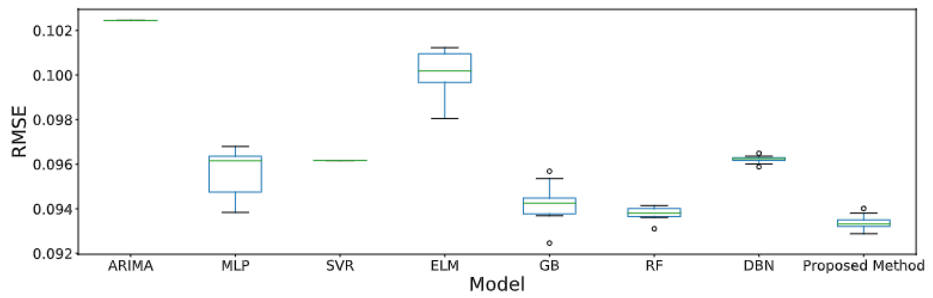
| Florianópolis | ARIMA [32,33] | 0.1024 | 24.74 | 0.0746 | 0.2135 | 0.9478 |
| RF [69,70] | 0.0938 | 21.28 | 0.0671 | 0.1944 | 0.9547 | |
| GB [37,38] | 0.0942 | 20.36 | 0.0663 | 0.1876 | 0.9553 | |
| SVR [34,71] | 0.0962 | 20.43 | 0.0655 | 0.1754 | 0.9558 | |
| MLP [39,72] | 0.0956 | 20.76 | 0.0667 | 0.1850 | 0.9548 | |
| ELM [40,41] | 0.1002 | 22.44 | 0.0713 | 0.2067 | 0.9499 | |
| DBN [42,43] | 0.0962 | 22.00 | 0.0693 | 0.1970 | 0.9531 | |
| HetDS(1,5) | 0.0955 | 20.68 | 0.0665 | 0.1840 | 0.9550 | |
| HetDS(1,10) | 0.0955 | 20.82 | 0.0670 | 0.1839 | 0.9550 | |
| HetDS(1,20) | 0.0938 | 20.52 | 0.0655 | 0.1791 | 0.9565 | |
| HetDS(3,5) | 0.0937 | 20.03 | 0.0648 | 0.1800 | 0.9564 | |
| HetDS(3,10) | 0.0934 | 19.87 | 0.0645 | 0.1788 | 0.9567 | |
| HetDS(3,20) | 0.0931 | 19.87 | 0.0643 | 0.1780 | 0.9570 | |
| HetDS(5,5) | 0.0934 | 19.97 | 0.0646 | 0.1802 | 0.9566 | |
| HetDS(5,10) | 0.0933 | 19.97 | 0.0645 | 0.1801 | 0.9566 | |
| HetDS(5,20) | 0.0933 | 19.95 | 0.0646 | 0.1805 | 0.9566 | |
| Hetmean | 0.0933 | 20.28 | 0.0648 | 0.1819 | 0.9564 | |
| Hetmedian | 0.0936 | 20.30 | 0.0650 | 0.1820 | 0.9563 | |
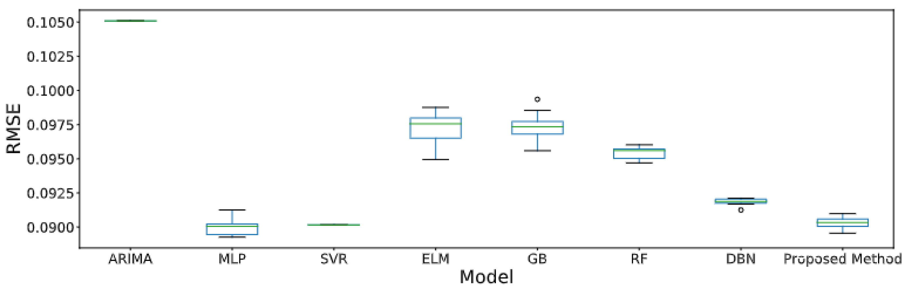
| Salvador | ARIMA [32,33] | 0.1051 | 27.15 | 0.0788 | 0.2739 | 0.9398 |
| RF [69,70] | 0.0954 | 19.48 | 0.0657 | 0.2102 | 0.9524 | |
| GB [37,38] | 0.0973 | 20.18 | 0.0668 | 0.2190 | 0.9504 | |
| SVR [34,71] | 0.0902 | 17.12 | 0.0579 | 0.1581 | 0.9610 | |
| MLP [39,72] | 0.0900 | 17.95 | 0.0601 | 0.1678 | 0.9599 | |
| ELM [40,41] | 0.0972 | 20.48 | 0.0666 | 0.1866 | 0.9541 | |
| DBN [42,43] | 0.0918 | 19.38 | 0.0632 | 0.1822 | 0.9573 | |
| HetDS(1,5) | 0.0935 | 18.28 | 0.0619 | 0.1804 | 0.9568 | |
| HetDS(1,10) | 0.0945 | 18.37 | 0.0626 | 0.1855 | 0.9557 | |
| HetDS(1,20) | 0.0943 | 18.03 | 0.0619 | 0.1842 | 0.9559 | |
| HetDS(3,5) | 0.0907 | 17.60 | 0.0599 | 0.1743 | 0.9589 | |
| HetDS(3,10) | 0.0903 | 17.55 | 0.0597 | 0.1730 | 0.9592 | |
| HetDS(3,20) | 0.0902 | 17.30 | 0.0592 | 0.1714 | 0.9594 | |
| HetDS(5,5) | 0.0896 | 17.74 | 0.0596 | 0.1720 | 0.9597 | |
| HetDS(5,10) | 0.0894 | 17.64 | 0.0593 | 0.1705 | 0.9600 | |
| HetDS(5,20) | 0.0895 | 17.64 | 0.0593 | 0.1706 | 0.9599 | |
| Hetmean | 0.0903 | 18.53 | 0.0609 | 0.1792 | 0.9585 | |
| Hetmedian | 0.0898 | 18.05 | 0.0602 | 0.1740 | 0.9593 | |
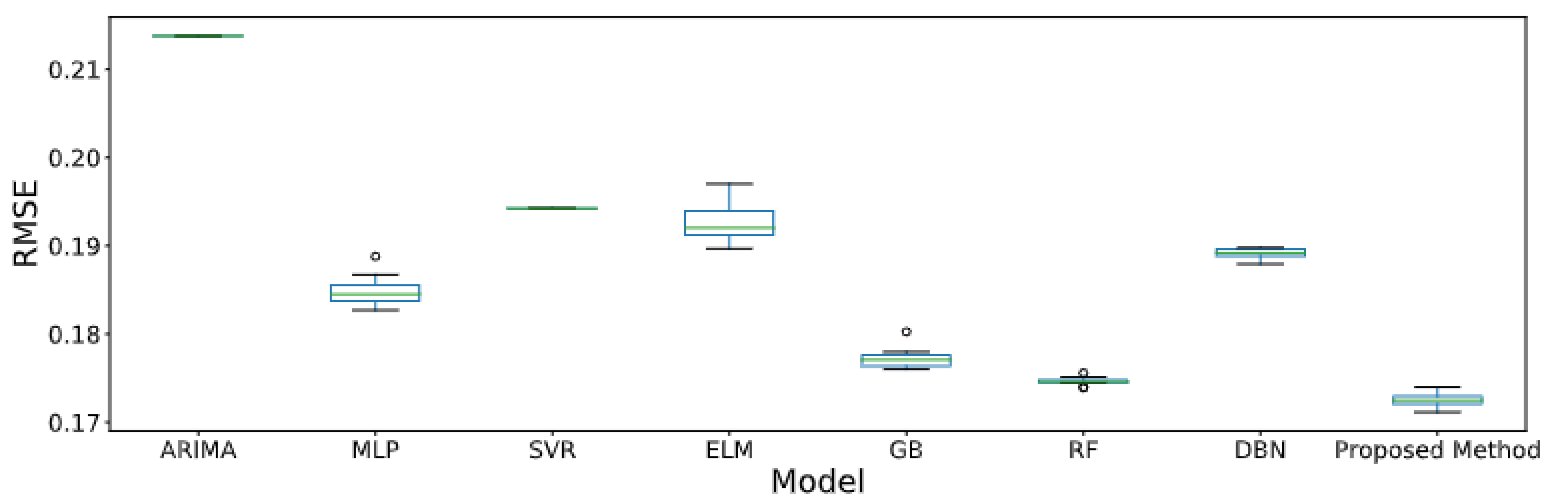
| São Paulo | ARIMA [32,33] | 0.2138 | 61.59 | 0.1456 | 1.2968 | 0.7355 |
| RF [69,70] | 0.1746 | 55.63 | 0.1173 | 0.9224 | 0.8215 | |
| GB [37,38] | 0.1772 | 53.20 | 0.1161 | 0.8342 | 0.8260 | |
| SVR [34,71] | 0.1942 | 55.88 | 0.1211 | 0.8148 | 0.8083 | |
| MLP [39,72] | 0.1849 | 58.32 | 0.1257 | 0.8780 | 0.8115 | |
| ELM [40,41] | 0.1927 | 59.09 | 0.1304 | 0.9796 | 0.7919 | |
| DBN [42,43] | 0.1892 | 57.10 | 0.1263 | 1.0258 | 0.7917 | |
| HetDS(1,5) | 0.1864 | 54.57 | 0.1194 | 0.8251 | 0.8163 | |
| HetDS(1,10) | 0.1808 | 52.70 | 0.1156 | 0.7878 | 0.8267 | |
| HetDS(1,20) | 0.1797 | 52.28 | 0.1154 | 0.8031 | 0.8262 | |
| HetDS(3,5) | 0.1767 | 52.40 | 0.1155 | 0.8335 | 0.8261 | |
| HetDS(3,10) | 0.1726 | 51.90 | 0.1137 | 0.8118 | 0.8327 | |
| HetDS(3,20) | 0.1720 | 51.51 | 0.1132 | 0.8144 | 0.8332 | |
| HetDS(5,5) | 0.1777 | 53.80 | 0.1176 | 0.8814 | 0.8201 | |
| HetDS(5,10) | 0.1764 | 53.84 | 0.1171 | 0.8748 | 0.8224 | |
| HetDS(5,20) | 0.1762 | 53.85 | 0.1169 | 0.8730 | 0.8230 | |
| Hetmean | 0.1802 | 55.30 | 0.1205 | 0.9473 | 0.8113 | |
| Hetmedian | 0.1832 | 55.11 | 0.1208 | 0.9539 | 0.8070 |
| MODEL | SERIES | |||
|---|---|---|---|---|
| Fortaleza | Florianópolis | Salvador | São Paulo | |
| ARIMA [32,33] | 14.97 | 27.28 | 19.55 | 9.11 |
| RF [69,70] | 6.38 | 19.16 | 1.5 | 0.72 |
| GB [37,38] | 8.21 | 19.67 | 2.96 | 1.18 |
| SVR [34,71] | 0.89 | 4.67 | 11.45 | 3.18 |
| MLP [39,72] | 0.75 | 11.29 | 6.97 | 2.62 |
| ELM [40,41] | 8.11 | 16.55 | 10.74 | 7.03 |
| DBN [42,43] | 2.72 | 9.16 | 9.08 | 3.23 |
| Hetmean | 4.43 | 4.23 | 7.76 | 2.46 |
| Hetmedian | 5.43 | 2.88 | 4.86 | 2.47 |
Publisher’s Note: MDPI stays neutral with regard to jurisdictional claims in published maps and institutional affiliations. |
© 2022 by the authors. Licensee MDPI, Basel, Switzerland. This article is an open access article distributed under the terms and conditions of the Creative Commons Attribution (CC BY) license (https://creativecommons.org/licenses/by/4.0/).
Share and Cite
de O. Santos, D.S., Jr.; de Mattos Neto, P.S.G.; de Oliveira, J.F.L.; Siqueira, H.V.; Barchi, T.M.; Lima, A.R.; Madeiro, F.; Dantas, D.A.P.; Converti, A.; Pereira, A.C.; et al. Solar Irradiance Forecasting Using Dynamic Ensemble Selection. Appl. Sci. 2022, 12, 3510. https://doi.org/10.3390/app12073510
de O. Santos DS Jr., de Mattos Neto PSG, de Oliveira JFL, Siqueira HV, Barchi TM, Lima AR, Madeiro F, Dantas DAP, Converti A, Pereira AC, et al. Solar Irradiance Forecasting Using Dynamic Ensemble Selection. Applied Sciences. 2022; 12(7):3510. https://doi.org/10.3390/app12073510
Chicago/Turabian Stylede O. Santos, Domingos S., Jr., Paulo S. G. de Mattos Neto, João F. L. de Oliveira, Hugo Valadares Siqueira, Tathiana Mikamura Barchi, Aranildo R. Lima, Francisco Madeiro, Douglas A. P. Dantas, Attilio Converti, Alex C. Pereira, and et al. 2022. "Solar Irradiance Forecasting Using Dynamic Ensemble Selection" Applied Sciences 12, no. 7: 3510. https://doi.org/10.3390/app12073510