
AIR-YOLOv3: Aerial Infrared Pedestrian Detection via an Improved YOLOv3 with Network Pruning
by
 ,
,
Yanhua Shao
1,* ,
,
Xingping Zhang
1, 
Hongyu Chu
1,*,
Xiaoqiang Zhang
1,
Duo Zhang
1 and
Yunbo Rao
2 1
School of Information Engineering, Southwest University of Science and Technology, Mianyang 621010, China
2
School of Information and Software Engineering, University of Electronic Science and Technology of China, Chengdu 610054, China
*
Authors to whom correspondence should be addressed.
Appl. Sci. 2022, 12(7), 3627; https://doi.org/10.3390/app12073627
Submission received: 4 March 2022
/
Revised: 31 March 2022
/
Accepted: 1 April 2022
/
Published: 3 April 2022
(This article belongs to the Special Issue Robot Vision: Theory, Methods and Applications)
Abstract
:Aerial object detection acts a pivotal role in searching and tracking applications. However, the large model, limited memory, and computing power of embedded devices restrict aerial pedestrian detection algorithms’ deployment on the UAV (unmanned aerial vehicle) platform. In this paper, an innovative method of aerial infrared YOLO (AIR-YOLOv3) is proposed, which combines network pruning and the YOLOv3 method. Firstly, to achieve a more appropriate number and size of the prior boxes, the prior boxes are reclustered. Then, to accelerate the inference speed on the premise of ensuring the detection accuracy, we introduced Smooth-L1 regularization on channel scale factors, and we pruned the channels and layers with less feature information to obtain a pruned YOLOv3 model. Meanwhile, we proposed the self-built aerial infrared dataset and designed ablation experiments to perform model evaluation well. Experimental results show that the AP (average precision) of AIR-YOLOv3 is 91.5% and the model size is 10.7 MB (megabyte). Compared to the original YOLOv3, its model volume compressed by 228.7 MB, nearly 95.5 %, while the model AP decreased by only 1.7%. The calculation amount is reduced by about 2/3, and the inference speed on the airborne TX2 has been increased from 3.7 FPS (frames per second) to 8 FPS.
1. Introduction
Pedestrian detection in infrared (IR) aerial night vision has gradually become an important research direction in recent years, and is critically applied in the fields of object search, person re-identification [1], marine trash detection [2], intelligent driving [3], and so on [4].
In recent years, the rapid development of deep learning (DL) [5] has injected new blood into object detection. Thus, the deep-learning-based object detection method has become the mainstream [6]. Although various detection algorithms have been proposed successively, the unstructured scenarios are still the main challenge to these detection algorithms, such as rigid target deformation, rapid target movement, obstacle occlusion, and drastic light changes in real applications [7].
Specifically, for infrared aerial photography scenarios [8], due to the long detection distance for the ground and the uncertainty of imaging perspective, the target is severely deformed. Moreover, the size of the imageable area for a person is small in the aerial image. Thirdly, compared with visible light images, the object lacks rich structural and texture features, and the target scale is uncertain. The environment, such as buildings, trees, and other obstacles, can submerge the target in the background. It causes a severe reduction in the object’s signal-to-noise ratio, and increases the difficulty of separating foreground and background. Finally, real-time performance is one of the primary considerations in the reality application, and it requires the designed algorithm to run in real time on a mobile platform with small volume, low power consumption, and limited computing resources.
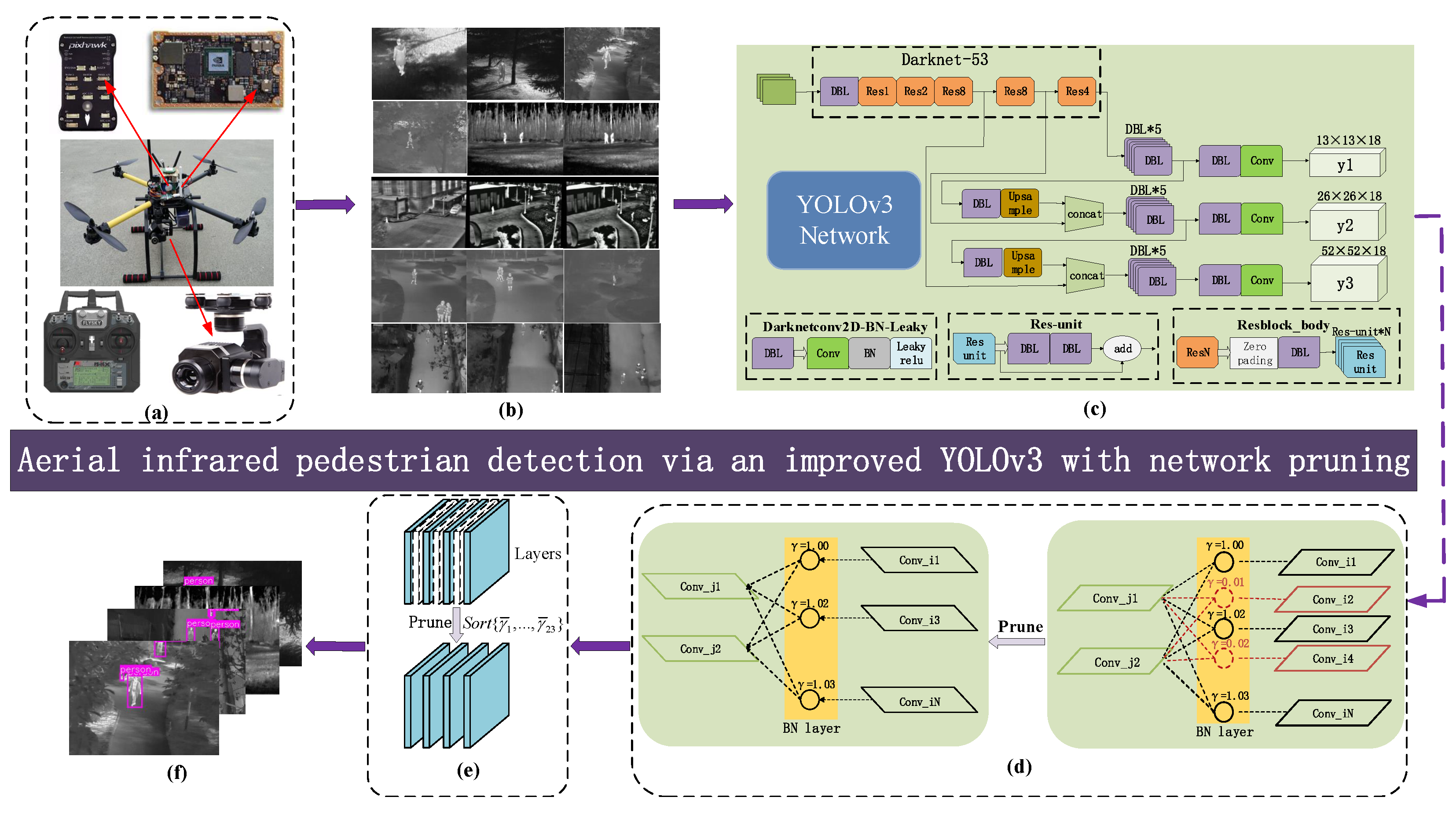
In this paper, an improved aerial infrared aerial YOLOv3 (AIR-YOLOv3) is proposed based on model pruning. The overall block diagram of the system is shown in Figure 1. Aerial infrared pedestrian data were collected through self-built tracking drones and were manually cleaned and marked. According to aerial data characteristics, the prior boxes of object are reclustered, and a more appropriate number and size of prior boxes are reselected. Based on the YOLOv3 model [9], we introduced the Smooth-L1 regularization on scale factor to sparse the model, and pruned channels and layers with small scale factor . The model is deployed on the airborne NVIDIA Jetson TX2.
Contributions and innovations of this paper are summarized as follows:
- An improved YOLOv3, AIR-YOLOv3, is proposed, which learns a more compact network structure by pruning [7], and it achieves a good trade-off between detection accuracy and inference speed.
- Since few published infrared-based aerial pedestrian datasets could be accessed, we constructed a new infrared aerial dataset, named the AIR-pedestrian dataset, that includes sample images in different scenarios.
- A UAV system was designed, and all the algorithms were implemented on the onboard Jetson TX2. The experimental results show that our proposed method can detect infrared pedestrians in public areas effectively.
The rest of this paper is organized as follows. This paper discusses related work in Section 2 below. Our proposed AIR-YOLOv3 method will be fully introduced in Section 3. Section 4 describes the experimental details. Finally, a short conclusion and discussion of this work are summarized in Section 5.
2. Related Work
In this section, we briefly survey relevant works, including common object detection, YOLO object detection methods, infrared and aerial object detection, and pruning.
2.1. Common Object Detection
Object detection is a long-standing, primary, and challenging problem in computer vision [10]. The goal of object detection is to determine in the image whether there are any object instances of given classes (such as humans, cars, dogs, or bottles), and if so, to return the spatial position and range of each object instance through a bounding box [11,12].
Since deep learning entered the field, there have appeared some milestone approaches, which are divided into two main categories: two-stage and one-stage [13]. Two-stage detectors usually have high localization and object recognition accuracy, while the one-stage detectors can achieve high inference speed [6]. For example, for the same graphics card, the FPS of YOLOv3 is generally four times that of faster R-CNN [14,15].
Two-stage detectors split the detection task into two stages, proposal generation and making predictions for these proposals. R-CNN series [16] are the landmark works of the two-stage method. They proposed RPN (region proposal network) to complete the detection task by an end-to-end neural network. A typical algorithm is mask R-CNN [16], which is an extended version of faster R-CNN and is an approach for object detection as well for instance segmentation.
2.2. YOLO
YOLOv1 [17] uses one CNN (convolutional neural network) model to achieve end-to-end object detection.
The most important improvement of YOLOv2 [20] is that the anchor mechanism is introduced to make object locating more precise and using a new backbone: darknet19. In darknet19, BN [21] (batch normalization) layers are added after convolution layers.
YOLOv3 [9] makes the network structure deeper by using the residual structure of ResNet [22]. In YOLOv3, there are three anchor boxes for each detect head. Moreover, there do not exist pooling layers and fully connected layers. YOLOv3 adopts FPN (feature pyramid networks) to achieve multi-scale detection, and it has three scale outputs, which are , , and , respectively.
2.3. Infrared Pedestrian Detection
With the development of deep learning, deep learning-based methods currently occupy the mainstream for infrared pedestrian detection [25].
In [25], the SSD algorithm was used for detecting pedestrians in infrared images, and embedded the SENet attention module into the network to reassign the weight of each feature channel to improve the network’s detection performance. Ref. [26] proposed a multi-spectral pedestrian detector to study the better fusion stages of the two-branch CNN, which combines visual–optical (VIS) image with infrared (IR) image, and makes it more adaptable to around-the-clock applications.
Dai et al. [27] firstly used a self-learning softmax with a nine-layer CNN model to identify near-infrared nighttime pedestrians. Testing results indicated that the optimized CNN model using self-learning softmax had a competitive accuracy and potential in real-time pedestrian recognition.
In [28], YOLO was used for person detection in thermal videos, and the performance of the standard YOLOv3 model is compared with a custom-trained model on a dataset of thermal images, which are extracted from videos recorded at night in clear weather, rain, and fog, and at different ranges with different types of movement: running, walking, and sneaking. Experimental results show that in all test scenarios, the average precision (AP) has excellent performance, and in thermal imaging with a modest training set, there is a significant improvement in person detection performance.
2.4. Network Pruning
Network pruning is widely used for reducing the heavy inference cost of deep models in low-resource settings, such as UAVs and other edge computing equipment [29]. A typical pruning process is a three-stage pipeline, i.e., training (a large model), pruning, and fine-tuning [30,31].
In early research, Gong et al. [32] showed that network pruning and quantization could effectively reduce network complexity. In [33], a simple magnitude-based three-step method was presented, including pruning, quantization, and Huffman coding, to remove the unimportant connections. Guo et al. [34] introduced dynamic network surgery to iteratively reduce the network’s complexity by pruning and splicing. In structured pruning, it prunes a complete structure, such as channels, filters, and layers. Li et al. [35] proposed the pruning of convolutional layer filters, which rank the filters according to their L1-norm and prune the low-ranking filters from each layer. Liu et al. [30] proposed a simple and effective method to prune channels, called network slimming. It directly adopted the BN layer scale factor as a pruning indicator and introduced L1 regularization to obtain a channel-wise sparsity model.
The network pruning is different from the compact network design and scale network in reducing the model. Compact network design is a method of choosing a small and compact network at the initial stage of model construction [30]. The most representative method is the MobileNet series [36]. Tiny-YOLOv3 is a designed compact network version of the original YOLOv3. Compared with other networks, these networks are smaller, faster, and less computational. However, considering the characteristics of infrared aerial photography data and the deployment of algorithms on mobile platforms, the algorithm’s robustness and its effective applications need further research. [29] implies that the pruned architecture itself, rather than a set of inherited ”important” weights, is more crucial to the efficiency of the final model. ”Lottery ticket hypothesis” [37,38] shows that finding effective subnetworks is significant for model compression. Facing a specific scene with limited data, it is quite difficult to design an effective network directly.
In scale networks [22,39,40,41], the higher accuracy is obtained by repeating feature networks [41]. When reducing these networks, this usually will reduce the effectiveness of the model. The pruned network after fine-tuning does not greatly reduce the accuracy and usually can achieve comparable detection accuracy to the original model.
3. AIR-YOLOv3
In terms of the limited computing capacity of the UAV, it is vital to balance model performance and high computation overhead.
We propose an improved YOLOv3, AIR-YOLOv3, which learns a more compact network structure by pruning to detect pedestrians in infrared images, as shown in Figure 1. Firstly, aerial infrared pedestrian data was captured through the self-built UAV, and it was manually cleaned and marked, as shown in Figure 1a,b. Secondly, according to aerial data characteristics, the object’s anchor boxes are reclustered, and a more appropriate number and size of anchor boxes are reselected. Third, we fine-tuned YOLOv3 on the self-build dataset, as shown in Figure 1c. Fourth, we imposed channel-wise sparsity by introducing Smooth-L1 regularization on scale factors and pruning the channels with less feature information, as shown in Figure 1d. After channel pruning, the layer pruning, as shown in Figure 1e, was carried out to further compress the model. Figure 1d,e show the processes of pruning optimization. Finally, the model is deployed on the airborne NVIDIA Jetson TX2.
The main optimization process of AIR-YOLOv3 is shown in Algorithm 1. The whole process is divided into three modules: (a) routine training, corresponding to steps 1 to 4; (b) sparse training, corresponding to steps 5 to 8; (c) channel pruning and layer pruning, corresponding to steps 9 to 13.
| Algorithm 1 Procedure of AIR-YOLOv3. |
| Input: the training set and the validation set Output: the pruned model
|
3.1. YOLOv3
3.1.1. Backbone
YOLOv3 utilizes a deeper network, DarkNet53, as the backbone to extract features, as shown in Figure 1c. DarkNet53 makes an incremental improvement to the previous backbone. It adds a BN layer behind each convolutional layer and upgrades the pooling layer. The residual structure is introduced to solve the problems, i.e., the deepened network is challenging to train, the network is difficult to converge, and the gradient explosion is to be prevented [22].
3.1.2. Logistic Classifier
Using the logistic classifier instead of the softmax loss function in YOLOv3 improves the single-label classification to multi-label classification. At the same time, the binary cross-entropy is used as the object confidence and class loss function, which can handle the multi-label classification well.
3.1.3. Multi-Scale Detection
The anchor boxes design still adopts the clustering algorithm, which is divided into three scales according to the labeled ground truth boxes. YOLOv3 utilizes the upsample and concat to achieve multi-scale feature fusion, and takes the three scales of feature map, which are , , and , respectively, to predict different scale objects.
The network structure of YOLOv3 is shown in Figure 1c. It contains the backbone network DarkNet53 and three detection headers. Furthermore, the composition and functions of the main modules are as follows:
- DBL (Darknetconv2D-BN-Leaky) modules are the main components of the network. They contain a convolutional layer, a batch normalization layer, and an activating layer. The convolutional layer and activating layer are connected by the BN layer in the whole network except the last convolutional layer in front of the detection header.
- Res-unit module is composed of two DBL modules and a residuals structure, which can effectively increase the network depth.
- ResN module is made up of N Res-units and a DBL module.
- Concat is tensor splicing. Unlike adding residual, it links the middle layer of darknet and the later upsample layer, which will change the output feature map’s dimension.
3.2. Bounding Box Clustering
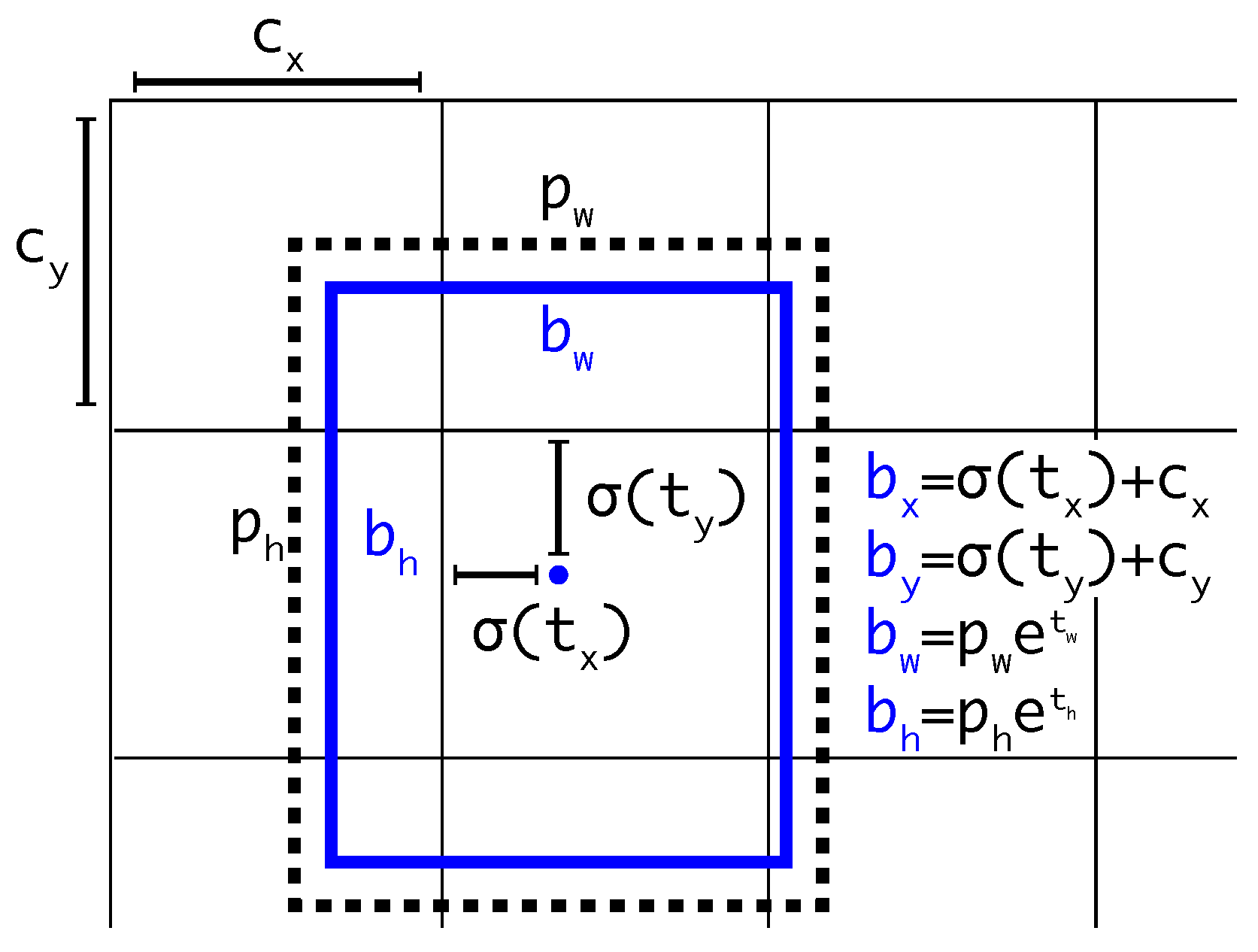
YOLOv3 is the quintessence of the YOLO series. The input image is divided into many grids, and every grid corresponds to predict three boxes. The prediction box of each object is deformed from the anchor box, which is clustered from the ground truth box of the . Specifically, during the model training, if the center of the prediction box is located in one grid cell, that grid cell is responsible for predicting. The box with the largest IOU (intersection over union) in the proposal boxes is used for predicting it. Furthermore, the final object bounding boxes are obtained by NMS (non-maximum suppression).
The prediction box is shown in Figure 2. , are the predicted offsets. , are the predicted scale parameters. The width and height of the bounding box prior are , , and the coordinates of the upper left corner of the grid cell are , .
This anchor-based method can effectively constrain the prediction box’s spatial scope, and add the prior knowledge to predict the box, which is conducive to converging the model. In origin YOLOv3, the K-means algorithm clusters nine anchor boxes through VOC and COCO image samples. These image samples contain multi-scale objects, which are not suitable for infrared aerial pedestrian data. Therefore, we clustered anchor boxes again according to the self-built aerial dataset to improve the matching degree between the prior boxes and pedestrian objects.
3.3. Network Pruning
The computing platform of UAVs always limits the performance of CNN-based object detection algorithms. In order to accelerate the inference on the premise of ensuring the model accuracy, we optimize the model by pruning channels and layers.
3.3.1. The Principle of Pruning
In darknet53, except for the three convolutions subsequently link to the YOLO detection header, each convolutional layer is followed by a BN layer to enable the model to converge quickly and prevent gradient explosion disappearance. The BN layer introduces a pair of parameters, and , which scale and shift the normalized input of the BN layer. Furthermore, the BN transformation is defined as
where is the BN layer output and and are scale factor and shift factor, respectively. means that when inputting mini-batch , we can obtain the result of the BN transform [21], which has two parameters and . is the result of the normalization of a mini-batch. is the current mini-batch input. and represent the mean and variance of the current mini-batch, respectively. is a constant added to variance for enhancing numerical stability.
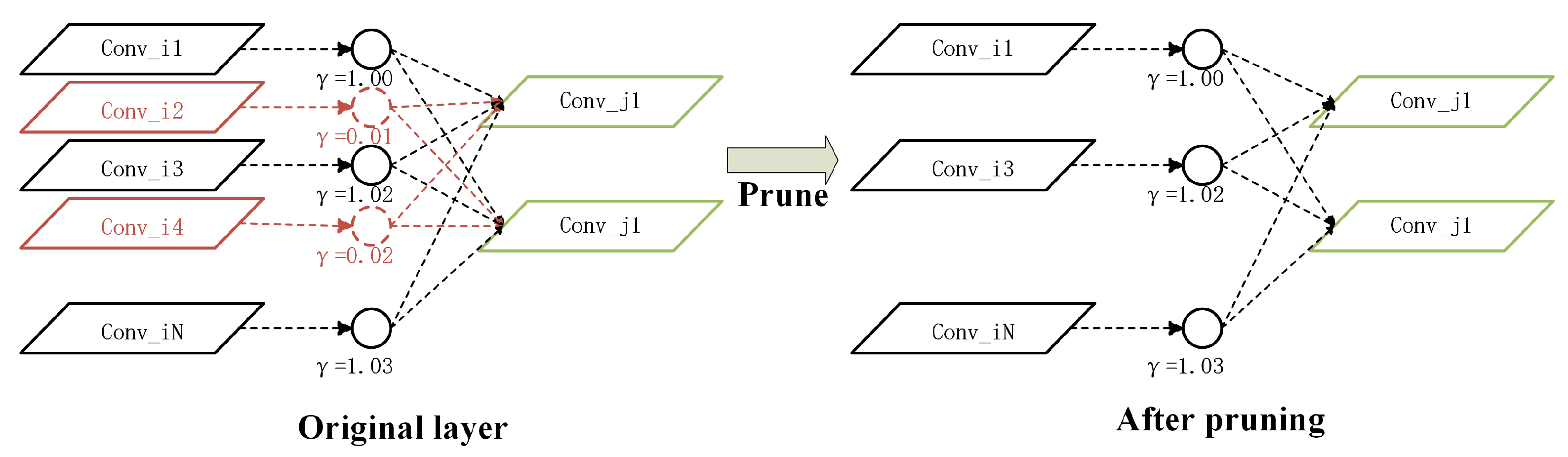
It can be seen that the output of the BN layer is related to and , which are learned along with the original model parameters. provides a measurement for CNN channels from Equation (1). Therefore, we can directly utilize the in BN layers as the scale factors to prune channels. We prune the CNN channels with the scale factor of the previous BN layer closer to zero. Moreover, we prune the layers based on the pruning channel to further obtain a smaller model. Specifically, we use the mean value of of the previous BN layer to measure the importance of the Res-unit and prune the Res-units.
3.3.2. Regularization and Sparse Training
In routine training, the values of close to zero occupy a minority ratio in the whole model, so it cannot obtain the high model compressing rate by pruning. Therefore, we introduce the regularization term to the original loss function to make some restrictions on the parameters with high complexity. This regularization term is introduced as the penalty of the , which pushes the of the unimportant channels toward zero.
Common regularization functions include L1 regularization function, known as the lasso regression: . L2 regularization function, known as the ridge regression, is , and Smooth-L1 regularization function is:
The derivative of L1 regularization function is a constant in the later period of training, leading to the training loss fluctuating around a stable value and difficulty to achieve higher accuracy. The derivative of L2 regularization function increases with x, resulting in the loss in the early period of training having a big gradient. The Smooth-L1 function has a smaller gradient when x is small. The upper gradient limit of Smooth-L1 is 1, making the training process more stable. Smooth-L1 regularization function is smooth at point zero. It can avoid the use of sub-gradient to solve extreme values at the non-smooth points and reduce the complexity of the model.
Regularization of the parameter by introducing the Smooth-L1 function can reduce the complexity of . Meanwhile, it pushes the factor value with less feature information toward zero. After introducing the Smooth-L1 regularization on , the network loss function during sparse training can be designed as follows:
where is the loss function of the original YOLOv3 [9]. is the regularization term on , where is a constant. It is the penalty of Smooth-L1 and a balance parameter between the original loss function and the introduced regularization term.
After sparse training, it can obtain the model with more scale factors closer to zero.
3.3.3. Channel Pruning and Layer Pruning
In the YOLOv3 network, there exist a total of 75 convolution layers. Except for the three convolutional layers in the front of the detection head and the two convolutional layers directly connected to the upsample layer, all the convolutional layers connect with the BN layer. Therefore, there exist 70 convolutional layers that can be pruned.
We arrange the of all the BN layers in order as . is a global threshold, which is obtained through the pruning ratio multiplied by the sorting result. At the same time, we give a local threshold in every convolution layer to prevent overpruning, and the is the minimum value within the maximum of every BN layer. The channels with scale factors smaller than and will be pruned.
There are five residual modules in YOLOv3, including 1, 2, 8, 8, 4 residual structures, respectively, and 23 residual structures in total. There exists a BN layer before every Res-unit. The average value of factor in this BN layer, , is used for evaluating the importance of the following residual network. As shown in Figure 3, we calculate and rank them. The residual structures with smaller will be pruned.
By pruning, we can obtain a more compact model with fewer parameters and less memory for running and inferencing. In the process of pruning channels, the pruning threshold will affect the compression ratio and generalization accuracy of the network model. Therefore, it is necessary to search for the most appropriate pruning threshold parameters through experiments. The high pruning ratio will decrease the detection accuracy of the compressed network, so we must fine-tune the compression model. Given the high similarity in the structure between the original model and the pruned model, we decided to use the transfer learning method to fine-tune the pruned model.
In real applications, the steps of the sparse train, prune, and fine-tune would be repeated until a prune model with suitable accuracy and desired compression ratio is obtained.
4. Experiment
4.1. Infrared Aerial Dataset
At present, most public datasets, such as ImageNet [12], VOC, and COCO, are not suitable for the application scene requirements of infrared aerial pedestrian detection. Therefore, we built an infrared aerial dataset, named the AIR-pedestrian. The class of the target is person.
An infrared camera is mounted on the four-rotor drone to capture pedestrian images in different scenes. The acquisition device is FLIR’s Vue Pro 336, which takes pictures of pedestrians at 5, 6, and 7 m at different flight altitudes to obtain infrared thermal images of different scales of pedestrians. The frame rate of captured video is 25 FPS, saved in AVI format. The resolution of a single frame is . Due to the high frame rate, images are obtained every five frames to contribute to the dataset.
Furthermore, in order to expand data and increase the diversity of data samples, some samples were introduced from the famous OTCBVS Benchmark Dataset via http://vcipl-okstate.org/pbvs/bench/ (accessed: 24 July 2021), without any other data augmentation. In addition to directly augmenting the dataset, transfer learning and pretraining weights can also be used, which can be understood as a form of indirectly augmenting the data [5,43].
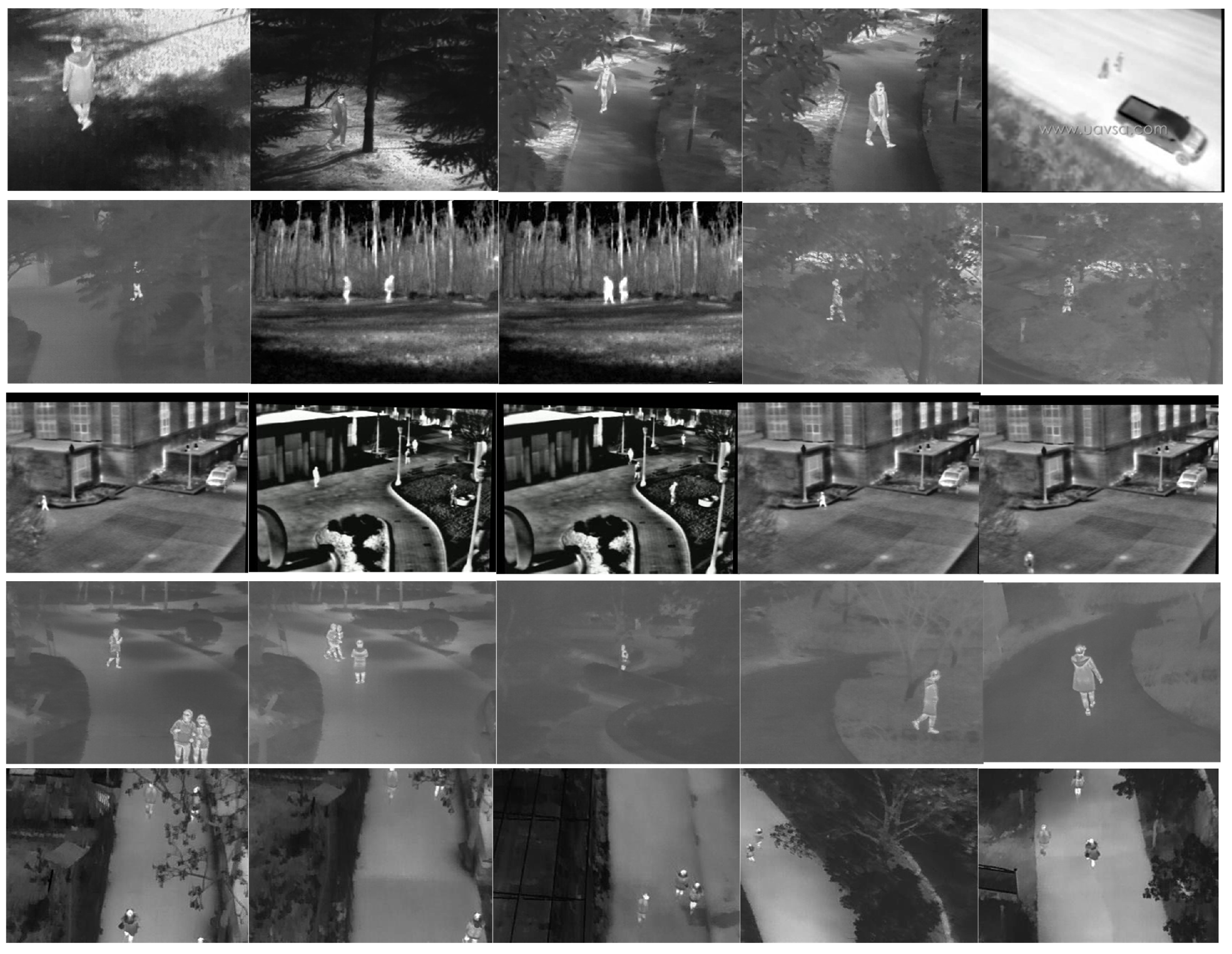
The AIR-pedestrian dataset includes different ages and gender of pedestrians, different numbers of pedestrians, and different occlusion degrees of pedestrians in different scenes, as shown in Figure 4.
The infrared dataset contains 2500 infrared aerial images and is divided into the training set and validation set . is used for the training detection model, is used for evaluating the model during training, and they do not intersect with each other. In the AIR-pedestrian dataset, 2000 images are used as , and 500 images are used as . Table 1 shows the scene distribution of the infrared aerial dataset.
4.2. Implementation Details
In our implementation, the penalty term is set to 0.001. The initial learning rate is set to 0.001. In the model training stage, we only used the data enhancement technology in literature [9]. The experimental hardware platform includes PC and Jetson TX2. The CPU of the PC is Intel i7-9750h, GPU is 6 GB GTX1660Ti, and uses PyTorch 1.2.0, OpenCV 3.4.3, and CUDA 10.0 without tensorRT. The Jetson TX2 uses Ubuntu 18.04, equipped with PyTorch 1.2.0 without tensorRT.
4.3. Sparse Training
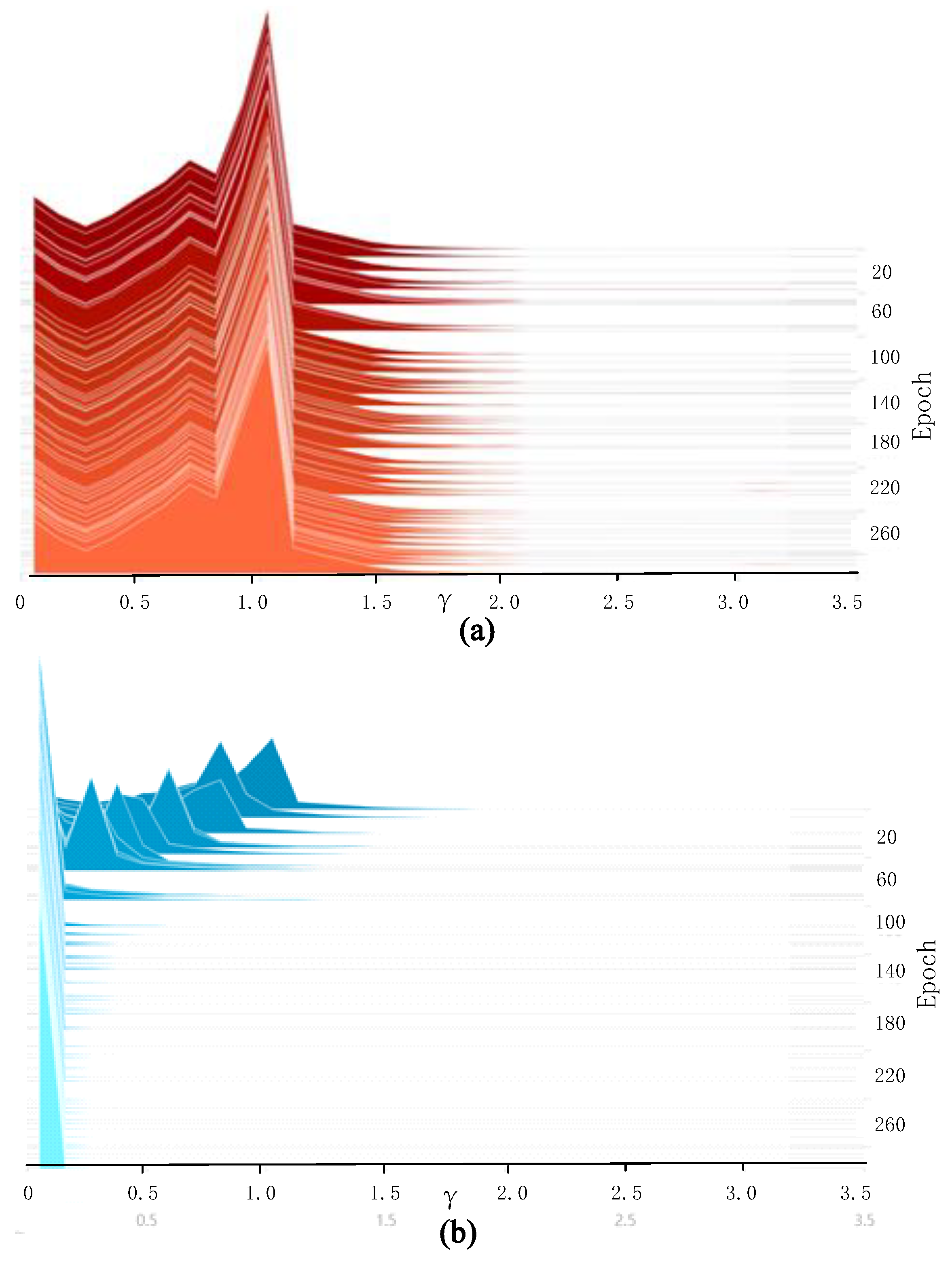
As shown in Figure 5, the vertical axis represents the total number of iterations of the samples, the horizontal axis is the value of the factor, and the graph height indicates the number of distribution in the corresponding value. In Figure 5a, is mostly distributed around 1 after routine training. The pruning cannot be carried out directly, so we introduce the regularization term.
Compared with [7] and [30], we introduce Smooth-L1 regularization instead of L1 because it can avoid using sub-gradient at non-smooth points. The experimental results show that Smooth-L1 regularization makes the scale factors decay more dramatically with the same training parameters. It may be possible to reduce the time consumption in a sparse training phase. In sparse training, the weight obtained from routine training is used as the pretraining model. After sparse training, the factor in the BN layer is pushed toward zero, and the distribution of the is shown in Figure 5.
4.4. Ablation Experiment
4.4.1. Anchor Boxes Reclustering
In order to determine the optimal number of anchor box K for infrared aerial data, we evaluate the optimal K according to the accuracy obtained by the K-means algorithm. The accuracy is the IOU between the candidate anchor boxes and the ground truth boxes. By setting different K, we compared the accuracy to determine the best number and the optimal size of anchor boxes.
As shown in Table 2, when K is set to 9, the IOU is 81.31%. This K is consistent with the anchor box of the original YOLOv3 algorithm, and the values are more suitable for infrared aerial pedestrian detection, which gives the model strong robustness.
4.4.2. Channel Pruning
After the sparse training, the value of the is pushed toward zero. The pruning ratio determines the number of pruned channels. is the channel pruning ratio and is defined as
where TP represents the number of pruned channels, and TC is the number of sparse model channels.
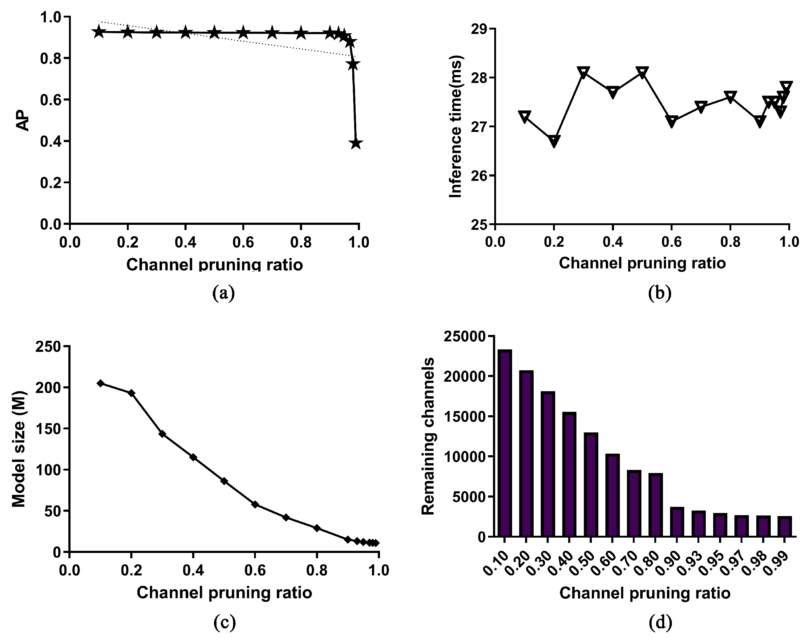
In order to find the optimal pruning ratio, we set different pruning ratios in the experiments. The trend of the model’s AP, inference time, model volume, and the number of remaining channels are shown in Figure 6.
In the experiment, we set the to 0%, 20%, 30%, 40%, 50%, 60%, 70%, 80%, 90%, 90%, 97%, 98%, and 99% to compare the model’s AP, inference time, model volume, and the number of pruned channels, respectively. Figure 6a shows that the model’s AP declined with the channel pruning ratio. Before the pruning ratio is set to 90%, the AP decreases slowly, basically remaining above 92%. When the pruning ratio exceeds 93%, the AP decreases rapidly. Figure 6b shows that the inference time fluctuates around 27 ms, regardless of the channel pruning ratio. Relatively speaking, the depth of the model has a greater effect on inference time [30].
From Figure 6c, it is obvious that with the channel pruning ratio increased, model size basically linearly declines.
Figure 6d is a bar chart of the number of remaining channels with different channel pruning ratios. Before the pruning ratio is set as 90%, the remaining channel is basically equal to the total number of channels (25,920) multiplied by the pruning ratio. After that, the channel number had little change due to the limitation of the local threshold , which is the minimum value within the maximum of every BN layer.
Through the above experiments, it can be determined that when the channel pruning ratio is about 90%, we can obtain a large compression rate with a small decrease in accuracy. Specifically, the compressed model size is 27.1 MB, and the size of the original model is 238.9. The model size decreased by 88.6%, while the accuracy is just reduced by 0.9%.
4.4.3. Layer Pruning
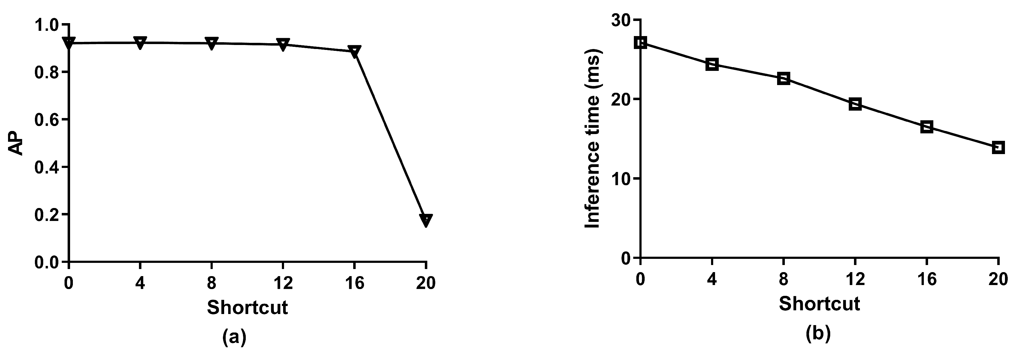
After channel pruning, the model size has been greatly compressed. However, the inference time of the model did not change significantly. After determining the optimal channel pruning ratio, we devote ourselves to finding the most suitable residual structure reduction quantity based on the optimal channel pruning ratio. We set five different numbers of pruned layers, which are 4, 8, 12, 16, and 20, respectively, to test the impact of different numbers of residual structures on AP and inference time.
Figure 7a is a line chart of the AP after pruning the residual structure. The horizontal axis represents the number of pruned residual structures and the vertical axis represents the AP of the model. With the increase in the number of pruned residual structures, the AP curve decreases smoothly. After the pruned number of residual structures exceeds 16, the AP curve decreases dramatically. In detail, when the quantity of pruned residual structures is 12, the detection accuracy decreases by 0.6%, and the inference time decreases by 8.6 ms. When the pruned residual quantity is 16, the AP decreases by 3.6%, and the inference time decreases by 11.1 ms. According to the application requirements, 12 is the best pruning residual structure number. Figure 7b is the curve of inference time. It can be seen that the model’s inference speed increases gradually with the increase of pruning layers. Through the above experiments, it can be found that layer pruning has a great influence on the model inference time, and the optimal number of pruning residual structures is 12.
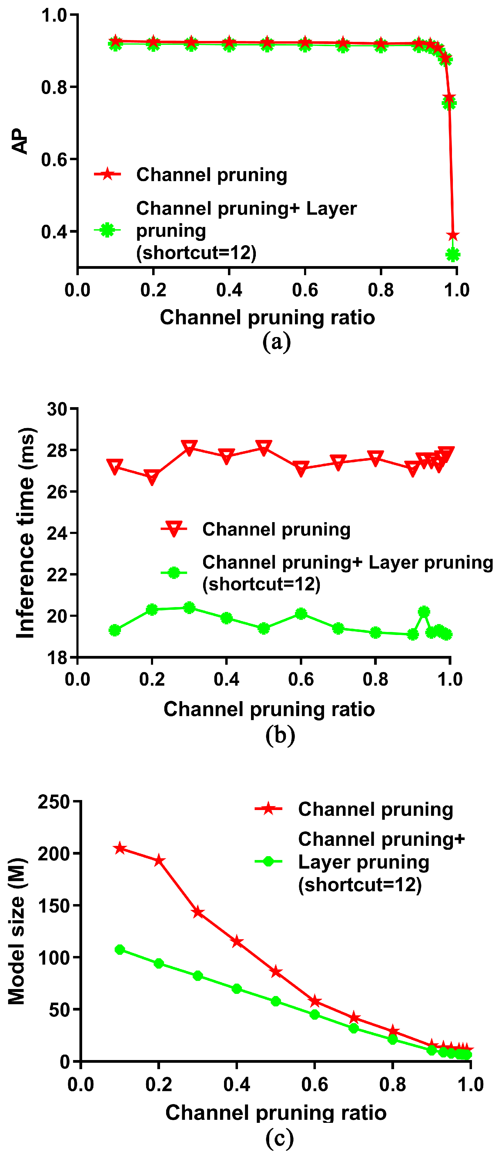
Figure 8 compares the effect of setting different channel pruning ratios when there is layer pruning and when there is no layer pruning. As shown in Figure 8a, the AP curve with layer pruning is consistent with the curve of only channel pruning. The channel pruning ratio of 90% is the inflection point of two curves, so the optimal pruning ratio is still 90%. Figure 8b is a change of inference time. After the channel pruning ratio exceeds 90%, the compression effect of the two models is similar, because the high pruning ratio means that the channels of convolution layers in the residual structure almost all become pruned, which is almost consistent with the layer pruning. The experimental results further indicate that the chosen parameters are optimal.
4.5. Model Test on PC and TX2
Experimental results show that the channel pruning ratio affects the compression rate significantly and the number of the pruned residual structures affects the inference time significantly. When the channel pruning ratio is 90% and the number of residual structures pruning is 12, we obtain the optimal model.
The quantitative comparison of mask R-CNN, YOLOv3, AIR-YOLOv3, and Tiny-YOLOv3 is shown in Table 3. The detection models were transplanted to the Jetson TX2, which is the most widely used embedded platform on UAVs because of its portability and low power consumption [44].
As shown in Table 3, the input size of the model is set to 416 × 416, which achieves the balance of detection speed and accuracy [9]. On the airborne TX2 compared with original YOLOv3 [9], the inference speed has been increased by nearly two times from 3.7 FPS to 8 FPS, and the model size is compressed by 228.2 MB, while the AP of the AIR-YOLOv3 is just 1.7% lower.
Compared with the well-known two-stage detection algorithm mask R-CNN [16], the inference speed on the airborne TX2 has been increased by nearly 11.4 times from 0.7 FPS to 8 FPS, while the AP of the AIR-YOLOv3 is just 4.0% lower. Compared with the Tiny-YOLOv3, which is the mobile version of YOLOv3, the AIR-YOLOv3 offers 18.1% higher AP, and 17.4 MB smaller model size.
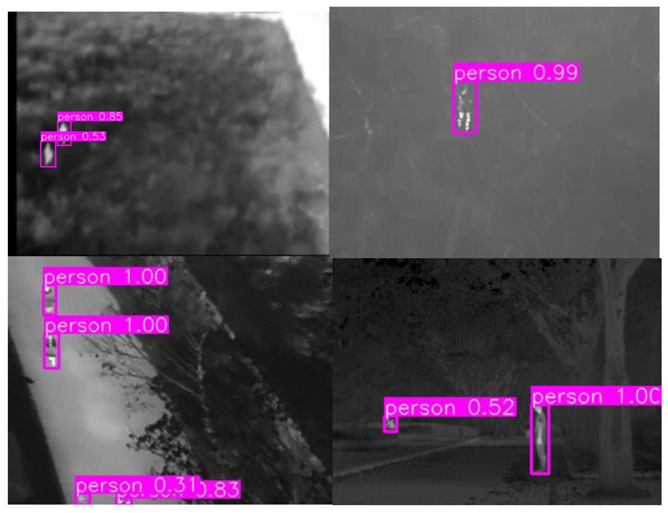
The AIR-YOLOv3 model runs on the Jetson TX2 to detect infrared pedestrian objects, and it can accurately predict the location of the object in the image, as shown in Figure 9.
In a word, AIR-YOLOv3 makes a good compromise for the detection accuracy and inference speed. At the same time, it has a smaller model size, which is conducive to the deployment on the mobile airborne computing platform.
5. Conclusions
Large models, limited memory, and computing power of embedded devices restrict the deployment of aerial pedestrian detection algorithms on the UAV platform. Therefore, an improved infrared aerial YOLOv3 (AIR-YOLOv3) is proposed. Firstly, given the aerial pedestrian dataset, the more suitable prior boxes are reclustered. Secondly, we impose the channel-wise sparsity on trained YOLOv3 model by introducing Smooth-L1 regularization on scale factors. Third, channel pruning was performed on the sparse model. Fourth, based on the channel pruned model, pruning layers were implemented to further compress the model. Finally, the compressed model was deployed on the airborne platform with NVIDIA Jetson TX2. Experiments have proved that the AIR-YOLOv3 achieves a great balance of system detection accuracy and speed, and the model is conducive to deployment on airborne mobile computing platforms.
Network pruning is an effective technique to deploy the large model on mobile devices. It is of great significance to the actual deployment of artificial intelligence algorithms. Choosing a better basic algorithm or a better pruning technique is an important research direction in the future. In addition, future work may be dedicated to pruning the network in a simpler and more flexible way and further exploring the CNN model acceleration technology on specific processor platforms.
Author Contributions
Conceptualization, Y.S. and X.Z. (Xingping Zhang); methodology, Y.S.; software, X.Z. (Xingping Zhang) and D.Z.; validation, Y.S. and X.Z. (Xingping Zhang); formal analysis, Y.S. and X.Z. (Xingping Zhang); investigation, Y.S. and X.Z. (Xingping Zhang); resources, Y.S. and H.C.; data curation, X.Z. (Xingping Zhang); writing—original draft preparation, X.Z. (Xingping Zhang); writing—review and editing, H.C. and X.Z. (Xiaoqiang Zhang); visualization, X.Z. (Xingping Zhang); supervision, H.C. and Y.R.; project administration, Y.S.; funding acquisition, Y.S. All authors have read and agreed to the published version of the manuscript.
Funding
This work was supported in part by the National Natural Science Foundation (NSFC) of China under Grant No. 61601382, Sichuan Provincial Science and Technology Support Project No. 2019YJ0325 and No. 2021YFG0314.
Data Availability Statement
More data and results are openly available in github at https://github.com/sunriselqq/IRA-YOLOv3 (Accessed: 27 March 2022).
Acknowledgments
The authors would like to thank the Senior AI Researcher Baivab Sinha in Sichuan Changhong Electric Co., Ltd., and all reviewers for very helpful comments and suggestions.
Conflicts of Interest
The authors declare no conflict of interest.
Abbreviations
The following abbreviations are used in this manuscript:
| IR | Infrared |
| AIR | Aerial infrared |
| UAV | Unmanned aerial vehicle |
| YOLO | You Look Only Once |
| FPS | Frames per second |
References
- Li, D.; Wei, X.; Hong, X.; Gong, Y. Infrared-Visible Cross-Modal Person Re-Identification with an X Modality. In Proceedings of the Thirty-Fourth AAAI Conference on Artificial Intelligence, AAAI 2020, New York, NY, USA, 7–12 February 2020; pp. 4610–4617. [Google Scholar]
- Liao, Y.H.; Juang, J.G. Real-Time UAV Trash Monitoring System. Appl. Sci. 2022, 12, 1838. [Google Scholar] [CrossRef]
- Park, J.; Chen, J.; Cho, Y.K.; Kang, D.Y.; Son, B.J. CNN-Based Person Detection Using Infrared Images for Night-Time Intrusion Warning Systems. Sensors 2020, 20, 34. [Google Scholar] [CrossRef] [PubMed] [Green Version]
- Xu, Z.; Zhuang, J.; Liu, Q.; Zhou, J.; Peng, S. Benchmarking a large-scale FIR dataset for on-road pedestrian detection. Infrared Phys. Technol. 2019, 96, 199–208. [Google Scholar] [CrossRef]
- LeCun, Y.; Bengio, Y.; Hinton, G. Deep learning. Nature 2015, 521, 436–444. [Google Scholar] [CrossRef] [PubMed]
- Jiao, L.; Zhang, F.; Liu, F.; Yang, S.; Li, L.; Feng, Z.; Qu, R. A survey of deep learning-based object detection. IEEE Access 2019, 7, 128837–128868. [Google Scholar] [CrossRef]
- Zhang, P.; Zhong, Y.; Li, X. SlimYOLOv3: Narrower, faster and better for real-time UAV applications. In Proceedings of the IEEE International Conference on Computer Vision Workshops, Seoul, Korea, 27–28 October 2019; pp. 37–45. [Google Scholar]
- Kanellakis, C.; Nikolakopoulos, G. Survey on Computer Vision for UAVs: Current Developments and Trends. J. Intell. Robot. Syst. 2017, 87, 141–168. [Google Scholar] [CrossRef] [Green Version]
- Redmon, J.; Farhadi, A. Yolov3: An incremental improvement. arXiv 2018, arXiv:1804.02767. [Google Scholar]
- Liu, L.; Ouyang, W.; Wang, X.; Fieguth, P.W.; Chen, J.; Liu, X.; Pietikäinen, M. Deep Learning for Generic Object Detection: A Survey. Int. J. Comput. Vis. 2020, 128, 261–318. [Google Scholar] [CrossRef] [Green Version]
- Everingham, M.; Gool, L.; Williams, C.K.; Winn, J.; Zisserman, A. The Pascal Visual Object Classes (VOC) Challenge. Int. J. Comput. Vis. 2010, 88, 303–338. [Google Scholar] [CrossRef] [Green Version]
- Russakovsky, O.; Deng, J.; Su, H.; Krause, J.; Satheesh, S.; Ma, S.; Huang, Z.; Karpathy, A.; Khosla, A.; Bernstein, M.; et al. Imagenet large scale visual recognition challenge. Int. J. Comput. Vis. 2015, 115, 211–252. [Google Scholar] [CrossRef] [Green Version]
- Wu, X.; Sahoo, D.; Hoi, S.C.H. Recent advances in deep learning for object detection. Neurocomputing 2020, 396, 39–64. [Google Scholar] [CrossRef] [Green Version]
- Bochkovskiy, A.; Wang, C.Y.; Liao, H.Y.M. YOLOv4: Optimal Speed and Accuracy of Object Detection. arXiv 2020, arXiv:2004.10934. [Google Scholar]
- Li, M.; Zhao, X.; Li, J.; Nan, L. ComNet: Combinational Neural Network for Object Detection in UAV-Borne Thermal Images. IEEE Trans. Geosci. Remote Sens. 2021, 59, 6662–6673. [Google Scholar] [CrossRef]
- He, K.; Gkioxari, G.; Dollár, P.; Girshick, R. Mask R-CNN. IEEE Trans. Pattern Anal. Mach. Intell. 2020, 42, 386–397. [Google Scholar] [CrossRef] [PubMed]
- Redmon, J.; Divvala, S.; Girshick, R.; Farhadi, A. You only look once: Unified, real-time object detection. In Proceedings of the IEEE Conference on Computer Vision and Pattern Recognition, IEEE Computer Society, Las Vegas, NV, USA, 26 July–1 June 2016; pp. 779–788. [Google Scholar]
- Liu, W.; Anguelov, D.; Erhan, D.; Szegedy, C.; Reed, S.; Fu, C.Y.; Berg, A.C. Ssd: Single shot multibox detector. In Proceedings of the European Conference on Computer Vision, Amsterdam, The Netherlands, 11–14 October 2016; pp. 21–37. [Google Scholar]
- Lin, T.Y.; Goyal, P.; Girshick, R.; He, K.; Dollár, P. Focal loss for dense object detection. IEEE Trans. Pattern Anal. Mach. Intell. 2020, 42, 318–327. [Google Scholar] [CrossRef] [PubMed] [Green Version]
- Redmon, J.; Farhadi, A. YOLO9000: Better, Faster, Stronger. In Proceedings of the 2017 IEEE Conference on Computer Vision and Pattern Recognition (CVPR), IEEE Computer Society, Honolulu, HI, USA, 21–26 July 2017; pp. 6517–6525. [Google Scholar]
- Ioffe, S.; Szegedy, C. Batch normalization: Accelerating deep network training by reducing internal covariate shift. In Proceedings of the International Conference on Machine Learning, Lille, France, 6–11 July 2015; pp. 448–456. [Google Scholar]
- He, K.; Zhang, X.; Ren, S.; Sun, J. Deep Residual Learning for Image Recognition. In Proceedings of the 2016 IEEE Conference on Computer Vision and Pattern Recognition (CVPR), IEEE Computer Society, Las Vegas, NV, USA, 27–30 June 2016; pp. 770–778. [Google Scholar]
- Wang, C.; Liao, H.M.; Wu, Y.; Chen, P.; Hsieh, J.; Yeh, I. CSPNet: A New Backbone that can Enhance Learning Capability of CNN. In Proceedings of the 2020 IEEE/CVF Conference on Computer Vision and Pattern Recognition, CVPR Workshops 2020 IEEE, Seattle, WA, USA, 14–19 June 2020; pp. 1571–1580. [Google Scholar] [CrossRef]
- Jocher, G.; Stoken, A.; Borovec, J.; NanoCode012; ChristopherSTAN; Changyu, L. Ultralytics/yolov5: v3.1—Bug Fixes and Performance Improvements; Zenodo: Genève, Switzerland, 2020. [Google Scholar] [CrossRef]
- Liu, X.; Li, F.; Liu, S. Improved SSD infrared image pedestrian detection algorithm. Electro Optics Control 2020, 20, 42–49. [Google Scholar]
- Pei, D.; Jing, M.; Liu, H.; Sun, F.; Jiang, L. A fast RetinaNet fusion framework for multi-spectral pedestrian detection. Infrared Phys. Technol. 2020, 105, 103178. [Google Scholar] [CrossRef]
- Dai, X.; Duan, Y.; Hu, J.; Liu, S.; Hu, C.; He, Y.; Chen, D.; Luo, C.; Meng, J. Near infrared nighttime road pedestrians recognition based on convolutional neural network. Infrared Phys. Technol. 2019, 97, 25–32. [Google Scholar] [CrossRef]
- Ivasic-Kos, M.; Kristo, M.; Pobar, M. Person Detection in Thermal Videos Using YOLO. In Proceedings of the Intelligent Systems and Applications 2019, London, UK, 5–6 September 2019; pp. 254–267. [Google Scholar] [CrossRef]
- Liu, Z.; Sun, M.; Zhou, T.; Huang, G.; Darrell, T. Rethinking the Value of Network Pruning. In Proceedings of the 7th International Conference on Learning Representations, ICLR 2019, New Orleans, LA, USA, 6–9 May 2019. [Google Scholar]
- Liu, Z.; Li, J.; Shen, Z.; Huang, G.; Yan, S.; Zhang, C. Learning efficient convolutional networks through network slimming. In Proceedings of the IEEE International Conference on Computer Vision, Venice, Italy, 22–29 October 2017; pp. 2736–2744. [Google Scholar]
- Zhang, X.; Zou, J.; He, K.; Sun, J. Accelerating Very Deep Convolutional Networks for Classification and Detection. IEEE Trans. Pattern Anal. Mach. Intell. 2016, 38, 1943–1955. [Google Scholar] [CrossRef] [Green Version]
- Gong, Y.; Liu, L.; Yang, M.; Bourdev, L. Compressing deep convolutional networks using vector quantization. arXiv 2014, arXiv:1412.6115. [Google Scholar]
- Han, S.; Mao, H.; Dally, W.J. Deep Compression: Compressing Deep Neural Network with Pruning, Trained Quantization and Huffman Coding. In Proceedings of the ICLR 2016, San Juan, Puerto Rico, 2–4 May 2016. [Google Scholar]
- Guo, Y.; Yao, A.; Chen, Y. Dynamic Network Surgery for Efficient DNNs. In Proceedings of the Advances in Neural Information Processing Systems 2016, Barcelona, Spain, 5–10 December 2016; pp. 1379–1387. [Google Scholar]
- Li, H.; Kadav, A.; Durdanovic, I.; Samet, H.; Graf, H.P. Pruning Filters for Efficient ConvNets. In Proceedings of the 5th International Conference on Learning Representations, ICLR 2017, Toulon, France, 24–26 April 2017. [Google Scholar]
- Howard, A.; Sandler, M.; Chu, G.; Chen, L.C.; Chen, B.; Tan, M.; Wang, W.; Zhu, Y.; Pang, R.; Vasudevan, V.; et al. Searching for mobilenetv3. In Proceedings of the IEEE/CVF International Conference on Computer Vision, IEEE Computer Society, Seoul, Korea, 27 October–2 November 2019; pp. 1314–1324. [Google Scholar]
- Frankle, J.; Carbin, M. The Lottery Ticket Hypothesis: Finding Sparse, Trainable Neural Networks. In Proceedings of the 7th International Conference on Learning Representations, ICLR 2019, New Orleans, LA, USA, 6–9 May 2019. [Google Scholar]
- Malach, E.; Yehudai, G.; Shalev-Schwartz, S.; Shamir, O. Proving the lottery ticket hypothesis: Pruning is all you need. In Proceedings of the International Conference on Machine Learning (ICML), Vienna, Austria, 13–18 July 2020; pp. 6682–6691. [Google Scholar]
- Tan, M.; Le, Q. Efficientnet: Rethinking model scaling for convolutional neural networks. In Proceedings of the International Conference on Machine Learning (ICML), Long Beach, CA, USA, 9–15 June 2019; pp. 6105–6114. [Google Scholar]
- Wang, C.Y.; Bochkovskiy, A.; Liao, H.Y.M. Scaled-YOLOv4: Scaling Cross Stage Partial Network. arXiv 2020, arXiv:2011.08036. [Google Scholar]
- Tan, M.; Pang, R.; Le, Q.V. Efficientdet: Scalable and efficient object detection. In Proceedings of the IEEE/CVF Conference on Computer Vision and Pattern Recognition, Seattle, WA, USA, 13–19 June 2020; pp. 10781–10790. [Google Scholar]
- Wu, D.; Lv, S.; Jiang, M.; Song, H. Using channel pruning-based YOLO v4 deep learning algorithm for the real-time and accurate detection of apple flowers in natural environments. Comput. Electron. Agric. 2020, 178, 105742. [Google Scholar] [CrossRef]
- Ganesh, P.; Chen, Y.; Yang, Y.; Chen, D.; Winslett, M. YOLO-ReT: Towards High Accuracy Real-time Object Detection on Edge GPUs. In Proceedings of the 2022 IEEE/CVF Winter Conference on Applications of Computer Vision (WACV), Waikoloa, HI, USA, 3–8 January 2022; pp. 1311–1321. [Google Scholar] [CrossRef]
- Rabah, M.; Rohan, A.; Haghbayan, M.H.; Plosila, J.; Kim, S.H. Heterogeneous Parallelization for Object Detection and Tracking in UAVs. IEEE Access 2020, 8, 42784–42793. [Google Scholar] [CrossRef]
Figure 1.
Overview of AIR-YOLOv3: (a) UAV system; (b) dataset construction; (c) fine-tuned YOLOv3 for aerial infrared pedestrian detection; (d) channel pruning; (e) layer pruning; and (f) test results.
Figure 1.
Overview of AIR-YOLOv3: (a) UAV system; (b) dataset construction; (c) fine-tuned YOLOv3 for aerial infrared pedestrian detection; (d) channel pruning; (e) layer pruning; and (f) test results.

Figure 2.
Bounding boxes with dimension priors and location prediction.

Figure 3.
Schematic diagram of channel pruning.

Figure 4.
The instance pictures of the AIR-pedestrian dataset. Each row from top to bottom represents the scene of daytime, woods, buildings, gardens, and roads, respectively.
Figure 4.
The instance pictures of the AIR-pedestrian dataset. Each row from top to bottom represents the scene of daytime, woods, buildings, gardens, and roads, respectively.

Figure 5.
Distribution of factor in the BN layer: (a) routine training and (b) sparse training.

Figure 6.
Influence of channel prune ratio: (a) AP curve, (b) inference time, (c) model size and (d) the number of channels.
Figure 6.
Influence of channel prune ratio: (a) AP curve, (b) inference time, (c) model size and (d) the number of channels.

Figure 7.
Influence of the number of the pruned residual structure: (a) AP curve and (b) inference time.
Figure 7.
Influence of the number of the pruned residual structure: (a) AP curve and (b) inference time.

Figure 8.
Influence of layer pruning and channel pruning: (a) AP curve, (b) inference time and (c) model size.
Figure 8.
Influence of layer pruning and channel pruning: (a) AP curve, (b) inference time and (c) model size.

Figure 9.
AIR-YOLOv3 test on TX2.The class of the target is person.


Table 1.
The distribution of scene.
| Scene | ||
|---|---|---|
| Daytime | 180 | 50 |
| Woods | 300 | 80 |
| Buildings | 550 | 150 |
| Garden | 300 | 70 |
| Road | 670 | 150 |
Table 2.
The accuracy analysis with different K values.
| k | Accuracy (%) | Anchors |
|---|---|---|
| 6 | 78.27 | (13,21), (21,49), (30,68), |
| (44,101), (9,20), (16,34) | ||
| 7 | 79.47 | (25,66), (16,34), (11,22) |
| (20,48), (53,113), (32,57), (36,83) | ||
| 8 | 79.86 | (44,101), (21,51), (19,20), (11,24) |
| (9,19), (30,68), (17,36), (14,30) | ||
| 9 | 81.31 | (16,35), (54,114), (38,86), (31,65) |
| (20,46), (13,28), (19,20), (10,21), (23,59) |
Publisher’s Note: MDPI stays neutral with regard to jurisdictional claims in published maps and institutional affiliations. |
© 2022 by the authors. Licensee MDPI, Basel, Switzerland. This article is an open access article distributed under the terms and conditions of the Creative Commons Attribution (CC BY) license (https://creativecommons.org/licenses/by/4.0/).
Share and Cite
MDPI and ACS Style
Shao, Y.; Zhang, X.; Chu, H.; Zhang, X.; Zhang, D.; Rao, Y. AIR-YOLOv3: Aerial Infrared Pedestrian Detection via an Improved YOLOv3 with Network Pruning. Appl. Sci. 2022, 12, 3627. https://doi.org/10.3390/app12073627
AMA Style
Shao Y, Zhang X, Chu H, Zhang X, Zhang D, Rao Y. AIR-YOLOv3: Aerial Infrared Pedestrian Detection via an Improved YOLOv3 with Network Pruning. Applied Sciences. 2022; 12(7):3627. https://doi.org/10.3390/app12073627
Chicago/Turabian StyleShao, Yanhua, Xingping Zhang, Hongyu Chu, Xiaoqiang Zhang, Duo Zhang, and Yunbo Rao. 2022. "AIR-YOLOv3: Aerial Infrared Pedestrian Detection via an Improved YOLOv3 with Network Pruning" Applied Sciences 12, no. 7: 3627. https://doi.org/10.3390/app12073627
Note that from the first issue of 2016, this journal uses article numbers instead of page numbers. See further details here.