Some FFT Algorithms for Small-Length Real-Valued Sequences

Abstract

This paper proposes fast algorithms for computing the discrete Fourier transform for real-valued sequences of lengths from 3 to 9. Since calculating the real-valued DFT using the complex-valued FFT is redundant regarding the number of needed operations, the developed algorithms do not operate on complex numbers. The algorithms are described in matrix–vector notation and their data flow diagrams are shown.

1. Introduction

Today, discrete Fourier transform (DFT) is one of the most popular digital signal- and image-processing tools [1,2,3,4,5,6,7]. However, it was used quite rarely for a long time due to its high computational complexity. In 1965, J. Cooley and J. Tukey proposed a fast algorithm to compute DFT with a drastically reduced number of arithmetical operations [8]. This discovery caused a furore among specialists and gave impetus to developing high-speed data processing algorithms based on fast Fourier transform (FFT). Mathematically, FFT algorithms are based on a factorization of the Fourier matrix into a product of sparse matrices, meaning matrices with many zero entries. In the case of the Cooley–Tukey algorithm, we are dealing with the representation of the original matrix as a product of ${log}_{2}N$ sparsely structured matrices. As is well known, the complexity of this algorithm is approximately $(N/2){log}_{2}N$ multiplications and the same number of additions of complex numbers.

In DFT algorithms, the input data is usually complex-valued. However, in practical digital signal-processing applications, the dataset for which the DFT is calculated is most often real-valued [9,10,11]. Therefore, developing algorithms suited explicitly for computing the DFT of real-valued data is an actual problem [12].

DFT algorithms for complex-valued data can be used directly for real-valued data. Specifically, the DFT of a real-valued dataset can be computed by converting it into a complex-valued dataset with zero imaginary parts. This approach, although simple, requires about twice the amount of computation and memory than that required in the case of more efficient algorithms designed for real-valued data. Moreover, ordinarily calculating the real-valued DFT using the complex-valued DFT is redundant regarding the number of operations performed. It is well known that the DFT of a real-valued signal is conjugate-symmetric. Therefore, even intuitively, one can assume that the calculations can be reduced by about half in this case. There are two main rational approaches to using the conventional complex-valued DFT to calculate the real-valued DFT. The first approach allows the simultaneous calculation of two N-point real-valued DFTs using a complex-valued DFT of the same size. The second approach is based on the transformation of an N-point real-valued sequence into an $N/2$-point complex-valued sequence, which leads to a reduction in computational complexity. Despite the existence of the mentioned approaches, there are a large number of algorithmic solutions developed specifically for real-valued data [12,13,14,15,16,17,18,19,20,21,22,23,24,25,26,27,28,29,30,31,32,33,34,35,36,37,38,39,40,41]. In this regard, articles [14,25,26] may be particularly noted.

The developed algorithms were presented mainly in algebraic relations, and less often in DFT matrix factorizations. However, none of the publications known to us explains how these ratios were obtained and from what considerations the presented matrices were constructed. This is especially true for small-length real-valued DFT algorithms. Thus, the details of constructing small-length real-valued DFT algorithms are essential. Nevertheless, the solutions given in the literature do not provide a complete imagination about the organization of the small-length real-valued DFT calculation process since their corresponding signal flow graphs are not presented anywhere. In addition, it should be noted that real-valued DFT algorithms for small-length sequences are described in publications available to the authors rather poorly [14].

Applications of short-size FFT algorithms are known from the literature [1,3,4,5,7]. The need to calculate real-valued DFTs arises, for example, in the world of the Internet of Things, smart sensors and connected devices generate a massive amount of data on petabytes per second. Due to communication costs that impact performance and energy consumption, there is an increasing need to perform a significant amount of computation closer to the edge rather than transferring large portions of raw data to the cloud. The latency and security risk of relying on the cloud is intolerable for applications deployed in drones, autonomous vehicles, robotics, and wearables. These applications are often enabled by DSP algorithms and, more specifically, by small-length real-valued DFTs, which extract meaningful information from raw data. Therefore, the efficient deployment of signal processing in embedded devices will improve near-sensor processing, avoid expensive data transmission, enable freedom from the cloud, and provide low latency and low energy consumption. This is a significant challenge due to the embedded systems resource constraints and the increased computational requirements of data processing.

The purpose of the article is to show the details of the organization of calculations of small-length DFTs for the case of real-valued input data as well as to reduce the number of arithmetic operations needed to compute the output.

Similar solutions for some $N(3,5,7)$ can be found in [14]. However, there are no considerations of how the presented matrices were constructed and the data flow diagrams are not shown. We have completed the missing algorithms for the remaining $N(4,6,8,9)$, described the way in which these algorithms were obtained, and shown the data flow diagrams for all N from 3 to 9.

2. Mathematical Background

The DFT of a discrete signal $x\left(n\right)$ of size N is given by

$$c\left(n\right)=\sum _{k=0}^{N-1}x\left(k\right)exp\frac{-j2\pi nk}{N}=\sum _{k=0}^{N-1}x\left(k\right)\left(cos\frac{2\pi nk}{N}-jsin\frac{2\pi nk}{N}\right)$$

(1)

for $n=0,1,\dots ,N-1$, where j is the imaginary unit. Each coefficient $c\left(n\right)$ of DFT, as a complex number, can be written as a sum

$$c\left(n\right)=a\left(n\right)+jb\left(n\right)$$

(2)

where $a\left(n\right)$ and $b\left(n\right)$ are the a real part and an imaginary part of $c\left(n\right)$, respectively. For real signal $x\left(n\right)$

$$a\left(n\right)=\sum _{k=0}^{N-1}x\left(k\right)cos\frac{2\pi nk}{N}$$

(3)

$$b\left(n\right)=-\sum _{k=0}^{N-1}x\left(k\right)sin\frac{2\pi nk}{N}$$

(4)

In this case, the DFT is redundant since it is conjugate-symmetric. Its real and imaginary parts meet the following properties:

$$a(N-n)=\sum _{k=0}^{N-1}x\left(k\right)cos\frac{2\pi (N-n)k}{N}=\sum _{k=0}^{N-1}x\left(k\right)cos\frac{2\pi nk}{N}=a\left(n\right)$$

(5)

$$b(N-n)=-\sum _{k=0}^{N-1}x\left(k\right)sin\frac{2\pi (N-n)k}{N}=\sum _{k=0}^{N-1}x\left(k\right)sin\frac{2\pi nk}{N}=-b\left(n\right)$$

(6)

Taking into account the periodicity of the signal $x\left(n\right)$ and their DFT with the period N, we can write

$$a(N-n)=a(-n)=a\left(n\right)$$

(7)

so the real part of DFT is an even function. Since

$$b(N-n)=b(-n)=-b\left(n\right)$$

(8)

then the imaginary part of DFT is an odd function. From (8) for $n=0$ we have $b(-0)=b\left(0\right)=-b\left(0\right)$, so we obtain

$$b\left(0\right)=0$$

(9)

and if N is an even number $b(N/2)=b(N-N/2)=b(-N/2)=-b(N/2)$, so

$$b\left(\frac{N}{2}\right)=0$$

(10)

In order to avoid redundancy and to use real transform for real signals the real discrete Fourier transform (RDFT) has been defined [25]

$$y\left(n\right)=\sum _{k=0}^{N-1}x\left(k\right)cos\left(\frac{2\pi nk}{N}+\theta \left(n\right)\right)$$

(11)

where

$$\theta \left(n\right)=\left\{\begin{array}{cc}0\hfill & 0\le n\le \lfloor \frac{N}{2}\rfloor \hfill \\ \frac{\pi }{2}\hfill & \lfloor \frac{N}{2}\rfloor <n\le N-1\hfill \end{array}\right.$$

(12)

and $\lfloor ·\rfloor$ denotes the floor function.

To see the relationship between the RDFT and the DFT of the signal $x\left(n\right)$, it is better to write the RDFT in a slightly different form

$$y\left(n\right)=\left\{\begin{array}{cc}\sum _{k=0}^{N-1}x\left(k\right)cos\frac{2\pi nk}{N}\hfill & 0\le n\le \lfloor \frac{N}{2}\rfloor \hfill \\ -\sum _{k=0}^{N-1}x\left(k\right)sin\frac{2\pi nk}{N}\hfill & \lfloor \frac{N}{2}\rfloor <n\le N-1\hfill \end{array}\right.$$

(13)

Now it is clear that

$$y\left(n\right)=\left\{\begin{array}{cc}a\left(n\right)\hfill & 0\le n\le \lfloor \frac{N}{2}\rfloor \hfill \\ b\left(n\right)\hfill & \lfloor \frac{N}{2}\rfloor <n\le N-1\hfill \end{array}\right.$$

(14)

so the RDFT contains the not repeated and non-zero coefficients from the real and imaginary parts of the DFT.

Knowing the RDFT coefficients of the signal and the relationships (7)–(10) and (14), it is easy to obtain the DFT coefficients. Namely, if N is an even number then

$$\begin{array}{c}a\left(0\right)=y\left(0\right)\hfill \\ a\left(1\right)=y\left(1\right)\hfill \\ ⋮\hfill \\ a(\frac{N}{2}-1)=y(\frac{N}{2}-1)\hfill \\ a\left(\frac{N}{2}\right)=y\left(\frac{N}{2}\right)\hfill \\ a(\frac{N}{2}+1)=a(\frac{N}{2}-1)=y(\frac{N}{2}-1)\hfill \\ ⋮\hfill \\ a(N-1)=a\left(1\right)=y\left(1\right)\hfill \end{array}\begin{array}{c}b\left(0\right)=0\hfill \\ b\left(1\right)=-b(N-1)=-y(N-1)\hfill \\ ⋮\hfill \\ b(\frac{N}{2}-1)=-b(\frac{N}{2}+1)=-y(\frac{N}{2}+1)\hfill \\ b\left(\frac{N}{2}\right)=0\hfill \\ b(\frac{N}{2}+1)=y(\frac{N}{2}+1)\hfill \\ ⋮\hfill \\ b(N-1)=y(N-1)\hfill \end{array}$$

(15)

If N is an odd number then

$$\begin{array}{c}a\left(0\right)=y\left(0\right)\hfill \\ a\left(1\right)=y\left(1\right)\hfill \\ ⋮\hfill \\ a\left(\frac{N-1}{2}\right)=y\left(\frac{N-1}{2}\right)\hfill \\ a\left(\frac{N+1}{2}\right)=a\left(\frac{N-1}{2}\right)=y\left(\frac{N-1}{2}\right)\hfill \\ ⋮\hfill \\ a(N-1)=a\left(1\right)=y\left(1\right)\hfill \end{array}\begin{array}{c}b\left(0\right)=0\hfill \\ b\left(1\right)=-b(N-1)=-y(N-1)\hfill \\ ⋮\hfill \\ b\left(\frac{N-1}{2}\right)=-b\left(\frac{N+1}{2}\right)=-y\left(\frac{N+1}{2}\right)\hfill \\ b\left(\frac{N+1}{2}\right)=y\left(\frac{N+1}{2}\right)\hfill \\ ⋮\hfill \\ b(N-1)=y(N-1)\hfill \end{array}$$

(16)

Later in the article, the matrix–vector notation will be used, so the discrete real input signal $x\left(n\right)$ of size N will be represented by a column vector ${\mathbf{x}}_N={[x_0,x_1,\dots ,x_{N-1}]}^T$, the N-by-N RDFT matrix will be denoted by ${\mathbf{R}}_N$ and the output signal $y\left(n\right)$—by ${\mathbf{y}}_N={[y_0,y_1,\dots ,y_{N-1}]}^T$, where ${[·]}^T$ means standard transposition operation. In matrix–vector notation the RDFT transform can be described as follows:

$${\mathbf{y}}_N={\mathbf{R}}_N{\mathbf{x}}_N$$

(17)

The entries $r_{nk}$ of the matrix ${\mathbf{R}}_N$ are obtained from (11)

$$r_{nk}=cos\left(\frac{2\pi nk}{N}+{\theta }_n\right)$$

(18)

where the indexes n and k vary from 0 to $N-1$ and ${\theta }_n=\theta \left(n\right)$ is defined by (12).

3. RDFT Algorithm for $\mathit{N}=\mathbf{3}$

For $N=2$, the DFT is real-valued for real input signal and it is the same as RDFT, so we will start from $N=3$. We introduce the denotation ${\varphi }_N=2\pi /N$. In this case the Equation (17) will take the form

$${\mathbf{y}}_3={\mathbf{R}}_3{\mathbf{x}}_3$$

(19)

where

$${\mathbf{R}}_3=\left[\begin{array}{ccc}cos0& cos0& cos0\\ cos0& cos{\varphi }_3& cos2{\varphi }_3\\ cos\frac{\pi }{2}& cos(2{\varphi }_3+\frac{\pi }{2})& cos(4{\varphi }_3+\frac{\pi }{2})\end{array}\right]=\left[\begin{array}{ccc}1& 1& 1\\ 1& cos{\varphi }_3& cos2{\varphi }_3\\ 0& -sin2{\varphi }_3& -sin4{\varphi }_3\end{array}\right]$$

(20)

Since ${\varphi }_3=2\pi /3$ then using the trigonometric reduction formulas we obtain $cos2{\varphi }_3=cos{\varphi }_3$, $sin2{\varphi }_3=-sin{\varphi }_3$, and $sin4{\varphi }_3=sin{\varphi }_3$, so the ${\mathbf{R}}_3$ matrix will take the form

$${\mathbf{R}}_3=\left[\begin{array}{ccc}1& 1& 1\\ 1& cos{\varphi }_3& cos{\varphi }_3\\ 0& sin{\varphi }_3& -sin{\varphi }_3\end{array}\right]$$

(21)

When we calculate the product of this matrix by the input vector ${\mathbf{x}}_3$ we obtain

$$\left[\begin{array}{c}{y}_0\\ y_1\\ y_2\end{array}\right]=\left[\begin{array}{c}{x}_0+(x_1+x_2)\\ x_0+cos{\varphi }_3(x_1+x_2)\\ sin{\varphi }_3(x_1-x_2)\end{array}\right]=\left[\begin{array}{c}{x}_0+(x_1+x_2)\\ (cos{\varphi }_3-1)(x_1+x_2)+[x_0+(x_1+x_2)]\\ sin{\varphi }_3(x_1-x_2)\end{array}\right]$$

(22)

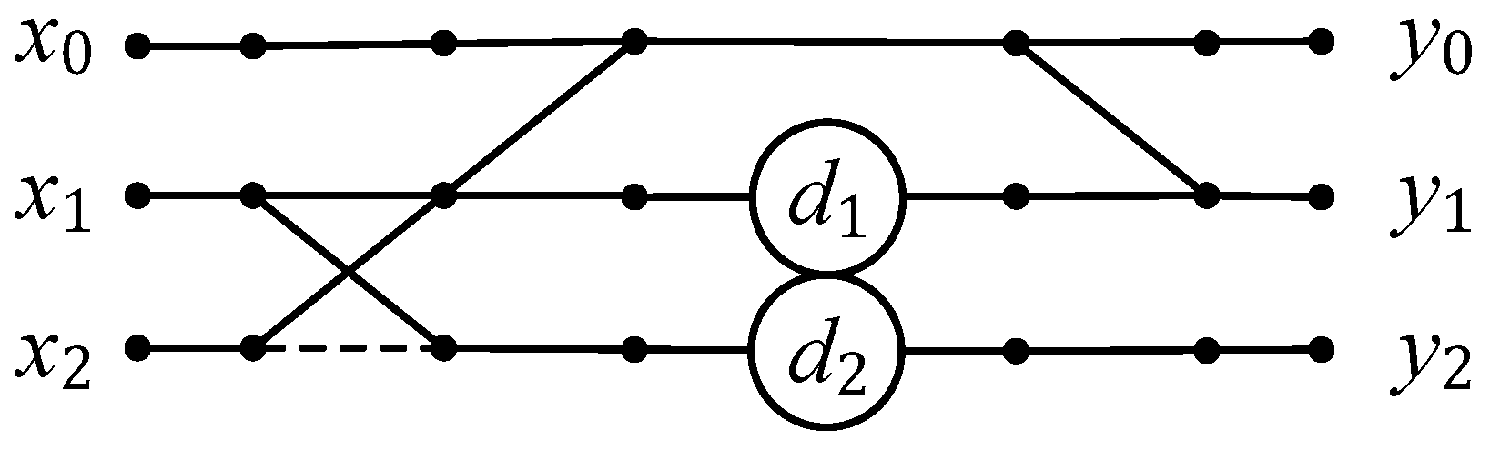
Figure 1 shows a data flow diagram corresponding to this calculation, where $d_1=cos{\varphi }_3-1$ and $d_2=sin{\varphi }_3$.

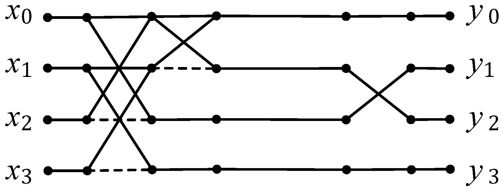
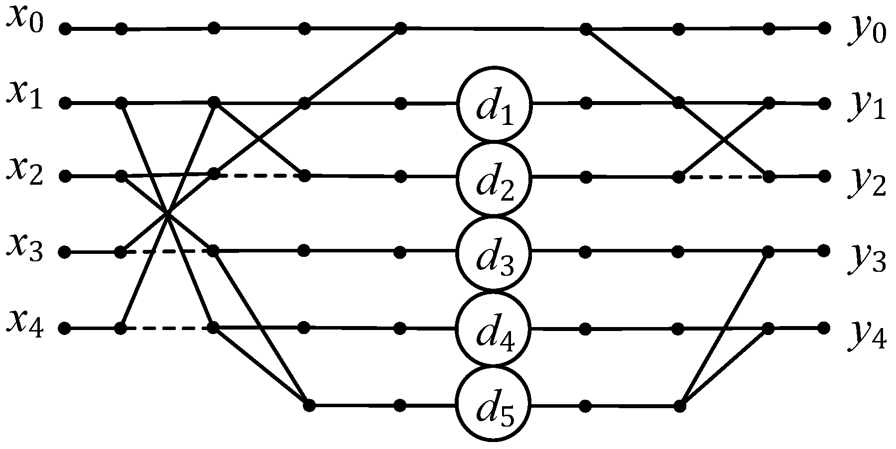
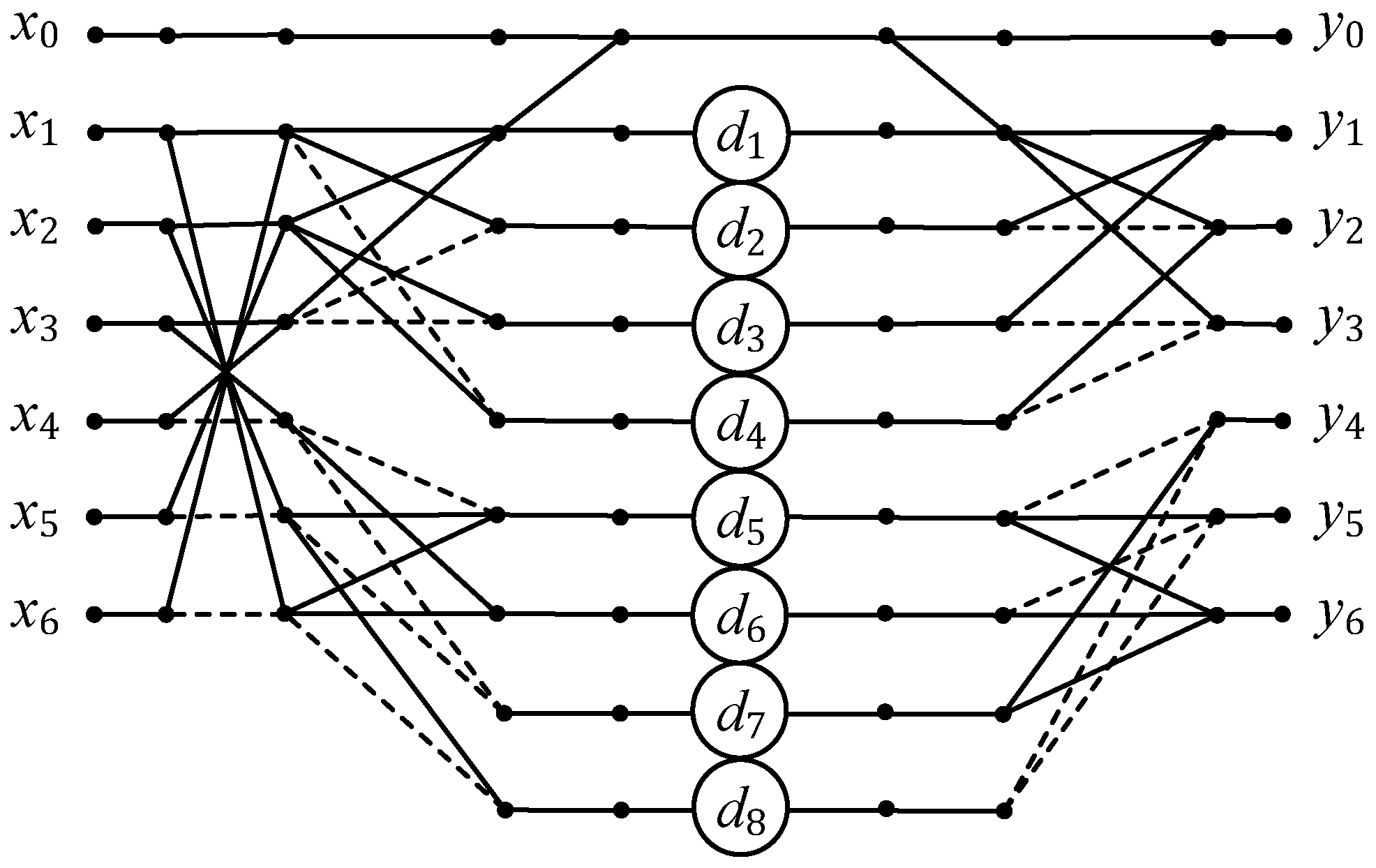
In this paper, data flow diagrams are oriented from left to right. Straight lines in the figures denote the operations of data transfer. Points where lines converge denote summation. The dotted lines indicate a signed-changed data transfer operation. The circles in these figures show the operation of multiplication by a number inscribed inside a circle.

When the vector ${\mathbf{z}}_3={\mathbf{a}}_3+i{\mathbf{b}}_3$ of complex coefficients of DFT for the real input vector ${\mathbf{x}}_3$ is needed, it can be easily obtained from the output vector ${\mathbf{y}}_3$ of RDFT, according to (16)

$${\mathbf{a}}_3=\left[\begin{array}{c}{a}_0\\ a_1\\ a_2\end{array}\right]=\left[\begin{array}{c}{y}_0\\ y_1\\ y_1\end{array}\right]{\mathbf{b}}_3=\left[\begin{array}{c}{b}_0\\ b_1\\ b_2\end{array}\right]=\left[\begin{array}{c}0\\ -y_2\\ y_2\end{array}\right]$$

(23)

The algorithm of the RDFT for $N=3$, presented in Figure 1, can be described by the following matrix–vector procedure, in which the matrix ${\mathbf{R}}_3$ has been factorized:

$${\mathbf{y}}_3={\mathbf{C}}_3{\mathbf{D}}_3{\tilde{\mathbf{A}}}_3{\widehat{\mathbf{A}}}_3{\mathbf{y}}_3$$

(24)

where

$${\widehat{\mathbf{A}}}_3=\left[\begin{array}{ccc}1& 0& 0\\ 0& 1& 1\\ 0& 1& -1\end{array}\right]{\tilde{\mathbf{A}}}_3=\left[\begin{array}{ccc}1& 1& 0\\ 0& 1& 0\\ 0& 0& 1\end{array}\right]{\mathbf{D}}_3=\left[\begin{array}{ccc}1& 0& 0\\ 0& d_1& 0\\ 0& 0& d_2\end{array}\right]{\mathbf{C}}_3=\left[\begin{array}{ccc}1& 0& 0\\ 1& 1& 0\\ 0& 0& 1\end{array}\right]$$

(25)

According to this algorithm we need only 2 multiplications and 4 additions of real numbers to calculate the output vector ${\mathbf{y}}_3$. It should be noted that only the matrix ${\mathbf{D}}_3$ is responsible for multiplications and that matrix is diagonal

$${\mathbf{D}}_3=\mathrm{diag}(1,d_1,d_2)$$

(26)

4. RDFT Algorithm for $\mathit{N}=\mathbf{4}$

For $N=4$, the Equation (17) will take the form

$${\mathbf{y}}_4={\mathbf{R}}_4{\mathbf{x}}_4$$

(27)

where

$${\mathbf{R}}_4=\left[\begin{array}{cccc}1& 1& 1& 1\\ 1& cos{\varphi }_4& cos2{\varphi }_4& cos3{\varphi }_4\\ 1& cos2{\varphi }_4& cos4{\varphi }_4& cos6{\varphi }_4\\ 0& -sin3{\varphi }_4& -sin6{\varphi }_4& -sin9{\varphi }_4\end{array}\right]$$

(28)

Since ${\varphi }_4=2\pi /4=\pi /2$ then $cos{\varphi }_4=0$, $cos2{\varphi }_4=-1$, $cos3{\varphi }_4=0$, $cos4{\varphi }_4=1$, $cos6{\varphi }_4=-1$ and $sin3{\varphi }_4=-1$, $sin6{\varphi }_4=0$, $sin9{\varphi }_4=1$, so the ${\mathbf{R}}_4$ matrix will take the form

$${\mathbf{R}}_4=\left[\begin{array}{cccc}1& 1& 1& 1\\ 1& 0& -1& 0\\ 1& -1& 1& -1\\ 0& 1& 0& -1\end{array}\right]$$

(29)

When we calculate the product of this matrix by the real input vector ${\mathbf{x}}_4$ we obtain

$$\left[\begin{array}{c}{y}_0\\ y_1\\ y_2\\ y_3\end{array}\right]=\left[\begin{array}{c}(x_0+x_2)+(x_1+x_3)\\ x_0-x_2\\ (x_0+x_2)-(x_1+x_3)\\ x_1-x_3\end{array}\right]$$

(30)

Figure 2 shows a data-flow diagram corresponding to this calculation.

When the vector ${\mathbf{z}}_4={\mathbf{a}}_4+i{\mathbf{b}}_4$ of complex coefficients of DFT for the input vector ${\mathbf{x}}_4$ is needed, it can be easily obtained from the output vector ${\mathbf{y}}_4$ of RDFT, according to (15)

$${\mathbf{a}}_4=\left[\begin{array}{c}{a}_0\\ a_1\\ a_2\\ a_3\end{array}\right]=\left[\begin{array}{c}{y}_0\\ y_1\\ y_2\\ y_1\end{array}\right]{\mathbf{b}}_4=\left[\begin{array}{c}{b}_0\\ b_1\\ b_2\\ b_3\end{array}\right]=\left[\begin{array}{c}0\\ -y_3\\ 0\\ y_3\end{array}\right]$$

(31)

The algorithm of the RDFT for $N=4$, presented in Figure 2, can be described by the following matrix-vector procedure, in which the matrix ${\mathbf{R}}_4$ has been factorized:

$${\mathbf{y}}_4={\mathbf{C}}_4{\mathbf{D}}_4{\tilde{\mathbf{A}}}_4{\widehat{\mathbf{A}}}_4{\mathbf{x}}_4$$

(32)

where

$${\widehat{\mathbf{A}}}_4=\left[\begin{array}{cccc}1& 0& 1& 0\\ 0& 1& 0& 1\\ 1& 0& -1& 0\\ 0& 1& 0& -1\end{array}\right]{\tilde{\mathbf{A}}}_4=\left[\begin{array}{cccc}1& 1& 0& 0\\ 1& -1& 0& 0\\ 0& 0& 1& 0\\ 0& 0& 0& 1\end{array}\right]{\mathbf{D}}_4={\mathbf{I}}_4{\mathbf{C}}_4=\left[\begin{array}{cccc}1& 0& 0& 0\\ 0& 0& 1& 0\\ 0& 1& 0& 0\\ 0& 0& 0& 1\end{array}\right]$$

(33)

and ${\mathbf{I}}_k$ denotes the identity matrix of size k.

According to this algorithm, we need only 6 additions of real numbers to calculate the output vector ${\mathbf{y}}_4$. It should be noted that the matrix ${\mathbf{D}}_4$ is responsible for multiplications and that, in this case, this matrix is equal to identity matrix, so we need not any multiplications of real numbers.

5. RDFT Algorithm for $\mathit{N}=\mathbf{5}$

For $N=5$, the Equation (17) will take the form

$${\mathbf{y}}_5={\mathbf{R}}_5{\mathbf{x}}_5$$

(34)

where

$${\mathbf{R}}_5=\left[\begin{array}{ccccc}1& 1& 1& 1& 1\\ 1& cos{\varphi }_5& cos2{\varphi }_5& cos3{\varphi }_5& cos4{\varphi }_5\\ 1& cos2{\varphi }_5& cos4{\varphi }_5& cos6{\varphi }_5& cos8{\varphi }_5\\ 0& -sin3{\varphi }_5& -sin6{\varphi }_5& -sin9{\varphi }_5& -sin12{\varphi }_5\\ 0& -sin4{\varphi }_5& -sin8{\varphi }_5& -sin12{\varphi }_5& -sin16{\varphi }_5\end{array}\right]$$

(35)

Since ${\varphi }_5=2\pi /5$ then $cos3{\varphi }_5=cos2{\varphi }_5$, $cos4{\varphi }_5=cos{\varphi }_5$, $cos6{\varphi }_5=cos{\varphi }_5$, $cos8{\varphi }_5=cos2{\varphi }_5$ and $sin3{\varphi }_5=-sin2{\varphi }_5$, $sin4{\varphi }_5=-sin{\varphi }_5$, $sin6{\varphi }_5=sin{\varphi }_5$, $sin8{\varphi }_5=-sin2{\varphi }_5$, $sin9{\varphi }_5=-sin{\varphi }_5$, $sin12{\varphi }_5=sin2{\varphi }_5$, $sin16{\varphi }_5=sin{\varphi }_5$, so the ${\mathbf{R}}_5$ matrix will take the form

$${\mathbf{R}}_5=\left[\begin{array}{ccccc}1& 1& 1& 1& 1\\ 1& cos{\varphi }_5& cos2{\varphi }_5& cos2{\varphi }_5& cos{\varphi }_5\\ 1& cos2{\varphi }_5& cos{\varphi }_5& cos{\varphi }_5& cos2{\varphi }_5\\ 0& sin2{\varphi }_5& -sin{\varphi }_5& sin{\varphi }_5& -sin2{\varphi }_5\\ 0& sin{\varphi }_5& sin2{\varphi }_5& -sin2{\varphi }_5& -sin{\varphi }_5\end{array}\right]$$

(36)

When we calculate the product of this matrix by the input vector ${\mathbf{x}}_5$ we obtain

$$\left[\begin{array}{c}{y}_0\\ y_1\\ y_2\\ y_3\\ y_4\end{array}\right]=\left[\begin{array}{c}{x}_0+[(x_1+x_4)+(x_2+x_3)]\\ x_0+cos{\varphi }_5(x_1+x_4)+cos2{\varphi }_5(x_2+x_3)\\ x_0+cos2{\varphi }_5(x_1+x_4)+cos{\varphi }_5(x_2+x_3)\\ sin2{\varphi }_5(x_1-x_4)-sin{\varphi }_5(x_2-x_3)\\ sin{\varphi }_5(x_1-x_4)+sin2{\varphi }_5(x_2-x_3)\end{array}\right]$$

(37)

To better understand the construction of the RDFT algorithm for $N=5$, we will introduce the notations $t_1=x_1+x_4$, $t_2=x_2+x_3$, $t_3=x_2-x_3$, $t_4=x_1-x_4$, $t_0=x_0+t_1+t_2$ and consider the sub-blocks of the output vector ${\mathbf{y}}_5$. The first sub-block is

$$\left[\begin{array}{c}{y}_1\\ y_2\end{array}\right]=\left[\begin{array}{c}{x}_0\\ x_0\end{array}\right]+\left[\begin{array}{cc}cos{\varphi }_5& cos2{\varphi }_5\\ cos2{\varphi }_5& cos{\varphi }_5\end{array}\right]\left[\begin{array}{c}{t}_1\\ t_2\end{array}\right]=$$

$$=\left[\begin{array}{c}{x}_0\\ x_0\end{array}\right]+\left[\begin{array}{cc}1& 1\\ 1& -1\end{array}\right]\left[\begin{array}{cc}{\displaystyle \frac{cos{\varphi }_5+cos2{\varphi }_5}{2}}& 0\\ 0& {\displaystyle \frac{cos{\varphi }_5-cos2{\varphi }_5}{2}}\end{array}\right]\left[\begin{array}{cc}1& 1\\ 1& -1\end{array}\right]\left[\begin{array}{c}{t}_1\\ t_2\end{array}\right]$$

(38)

We can also write it as

$$\left[\begin{array}{c}{y}_1\\ y_2\end{array}\right]=\left[\begin{array}{c}{t}_0\\ t_0\end{array}\right]+\left[\begin{array}{cc}1& 1\\ 1& -1\end{array}\right]\left[\begin{array}{cc}{\displaystyle \frac{cos{\varphi }_5+cos2{\varphi }_5}{2}}-1& 0\\ 0& {\displaystyle \frac{cos{\varphi }_5-cos2{\varphi }_5}{2}}\end{array}\right]\left[\begin{array}{cc}1& 1\\ 1& -1\end{array}\right]\left[\begin{array}{c}{t}_1\\ t_2\end{array}\right]$$

(39)

The second sub-block is

$$\left[\begin{array}{c}{y}_3\\ y_4\end{array}\right]=\left[\begin{array}{cc}-sin{\varphi }_5& sin2{\varphi }_5\\ sin2{\varphi }_5& sin{\varphi }_5\end{array}\right]\left[\begin{array}{c}{t}_3\\ t_4\end{array}\right]=$$

$$=\left[\begin{array}{ccc}1& 0& 1\\ 0& 1& 1\end{array}\right]\left[\begin{array}{ccc}-sin{\varphi }_5-sin2{\varphi }_5& 0& 0\\ 0& sin{\varphi }_5-sin2{\varphi }_5& 0\\ 0& 0& sin2{\varphi }_5\end{array}\right]\left[\begin{array}{cc}1& 0\\ 0& 1\\ 1& 1\end{array}\right]\left[\begin{array}{c}{t}_3\\ t_4\end{array}\right]$$

(40)

Figure 3 shows a data flow diagram corresponding to the calculation of the output vector, where $d_1=(cos{\varphi }_5+cos2{\varphi }_5)/2-1$, $d_2=(cos{\varphi }_5-cos2{\varphi }_5)/2$, $d_3=-sin{\varphi }_5-sin2{\varphi }_5$, $d_4=sin{\varphi }_5-sin2{\varphi }_5$ and $d_5=sin2{\varphi }_5$.

When the vector ${\mathbf{z}}_5={\mathbf{a}}_5+i{\mathbf{b}}_5$ of complex coefficients of DFT for the real input vector ${\mathbf{x}}_5$ is needed, it can be easily obtained from the output vector ${\mathbf{y}}_5$ of RDFT, according to (16)

$${\mathbf{a}}_5=\left[\begin{array}{c}{a}_0\\ a_1\\ a_2\\ a_3\\ a_4\end{array}\right]=\left[\begin{array}{c}{y}_0\\ y_1\\ y_2\\ y_2\\ y_1\end{array}\right]{\mathbf{b}}_5=\left[\begin{array}{c}{b}_0\\ b_1\\ b_2\\ b_3\\ b_4\end{array}\right]=\left[\begin{array}{c}0\\ -y_4\\ -y_3\\ y_3\\ y_4\end{array}\right]$$

(41)

The algorithm of the RDFT for $N=5$, presented in Figure 3, can be described by the following matrix–vector procedure, in which the matrix ${\mathbf{R}}_5$ has been factorized:

$${\mathbf{y}}_5={\mathbf{C}}_{5\times 6}{\tilde{\mathbf{C}}}_6{\mathbf{D}}_6{\tilde{\mathbf{A}}}_6{\overline{\mathbf{A}}}_{6\times 5}{\widehat{\mathbf{A}}}_5{\mathbf{x}}_5$$

(42)

where

$${\widehat{\mathbf{A}}}_5=\left[\begin{array}{ccccc}1& 0& 0& 0& 0\\ 0& 1& 0& 0& 1\\ 0& 0& 1& 1& 0\\ 0& 0& 1& -1& 0\\ 0& 1& 0& 0& -1\end{array}\right]{\overline{\mathbf{A}}}_{6\times 5}=\left[\begin{array}{ccccc}1& 0& 0& 0& 0\\ 0& 1& 1& 0& 0\\ 0& 1& -1& 0& 0\\ 0& 0& 0& 1& 0\\ 0& 0& 0& 0& 1\\ 0& 0& 0& 1& 1\end{array}\right]{\tilde{\mathbf{A}}}_6=\left[\begin{array}{cccccc}1& 1& 0& 0& 0& 0\\ 0& 1& 0& 0& 0& 0\\ 0& 0& 1& 0& 0& 0\\ 0& 0& 0& 1& 0& 0\\ 0& 0& 0& 0& 1& 0\\ 0& 0& 0& 0& 0& 1\end{array}\right]$$

(43)

$${\mathbf{D}}_6=\left[\begin{array}{cccccc}1& 0& 0& 0& 0& 0\\ 0& d_1& 0& 0& 0& 0\\ 0& 0& d_2& 0& 0& 0\\ 0& 0& 0& d_3& 0& 0\\ 0& 0& 0& 0& d_4& 0\\ 0& 0& 0& 0& 0& d_5\end{array}\right]{\tilde{\mathbf{C}}}_6=\left[\begin{array}{cccccc}1& 0& 0& 0& 0& 0\\ 1& 1& 0& 0& 0& 0\\ 0& 0& 1& 0& 0& 0\\ 0& 0& 0& 1& 0& 0\\ 0& 0& 0& 0& 1& 0\\ 0& 0& 0& 0& 0& 1\end{array}\right]{\mathbf{C}}_{5\times 6}=\left[\begin{array}{cccccc}1& 0& 0& 0& 0& 0\\ 0& 1& 1& 0& 0& 0\\ 0& 1& -1& 0& 0& 0\\ 0& 0& 0& 1& 0& 1\\ 0& 0& 0& 0& 1& 1\end{array}\right]$$

(44)

According to this algorithm we need only 13 additions and 5 multiplications of real numbers to calculate the output vector ${\mathbf{y}}_5$.

6. RDFT Algorithm for $\mathit{N}=\mathbf{6}$

For $N=6$, the Equation (17) will take the form

$${\mathbf{y}}_6={\mathbf{R}}_6{\mathbf{x}}_6$$

(45)

where

$${\mathbf{R}}_6=\left[\begin{array}{cccccc}1& 1& 1& 1& 1& 1\\ 1& cos{\varphi }_6& cos2{\varphi }_6& cos3{\varphi }_6& cos4{\varphi }_6& cos5{\varphi }_6\\ 1& cos2{\varphi }_6& cos4{\varphi }_6& cos6{\varphi }_6& cos8{\varphi }_6& cos10{\varphi }_6\\ 1& cos3{\varphi }_6& cos6{\varphi }_6& cos9{\varphi }_6& cos12{\varphi }_6& cos15{\varphi }_6\\ 0& -sin4{\varphi }_6& -sin8{\varphi }_6& -sin12{\varphi }_6& -sin16{\varphi }_6& -sin20{\varphi }_6\\ 0& -sin5{\varphi }_6& -sin10{\varphi }_6& -sin15{\varphi }_6& -sin20{\varphi }_6& -sin25{\varphi }_6\end{array}\right]$$

(46)

Since ${\varphi }_6=2\pi /6$ then $cos2{\varphi }_6=-cos{\varphi }_6$, $cos3{\varphi }_6=-1$, $cos4{\varphi }_6=-cos{\varphi }_6$, $cos5{\varphi }_6=cos{\varphi }_6$, $cos6{\varphi }_6=1$, $cos8{\varphi }_6=-cos{\varphi }_6$, $cos9{\varphi }_6=-1$, $cos10{\varphi }_6=-cos{\varphi }_6$, $cos12{\varphi }_6=1$, $cos15{\varphi }_6=-1$ and $sin4{\varphi }_6=-sin{\varphi }_6$, $sin5{\varphi }_6=-sin{\varphi }_6$, $sin8{\varphi }_6=sin{\varphi }_6$, $sin10{\varphi }_6=-sin{\varphi }_6$, $sin12{\varphi }_6=0$, $sin15{\varphi }_6=0$, $sin16{\varphi }_6=-sin{\varphi }_6$, $sin20{\varphi }_6=sin{\varphi }_6$, $sin25{\varphi }_6=sin{\varphi }_6$, so the ${\mathbf{R}}_6$ matrix will take the form

$${\mathbf{R}}_6=\left[\begin{array}{cccccc}1& 1& 1& 1& 1& 1\\ 1& cos{\varphi }_6& -cos{\varphi }_6& -1& -cos{\varphi }_6& cos{\varphi }_6\\ 1& -cos{\varphi }_6& -cos{\varphi }_6& 1& -cos{\varphi }_6& -cos{\varphi }_6\\ 1& -1& 1& -1& 1& -1\\ 0& sin{\varphi }_6& -sin{\varphi }_6& 0& sin{\varphi }_6& -sin{\varphi }_6\\ 0& sin{\varphi }_6& sin{\varphi }_6& 0& -sin{\varphi }_6& -sin{\varphi }_6\end{array}\right]$$

(47)

When we calculate the product of this matrix by the input vector ${\mathbf{x}}_6$ we obtain

$$\left[\begin{array}{c}{y}_0\\ y_1\\ y_2\\ y_3\\ y_4\\ y_5\end{array}\right]=\left[\begin{array}{c}(x_0+x_3)+(x_1+x_5)+(x_2+x_4)\\ (x_0-x_3)+cos{\varphi }_6[(x_1+x_5)-(x_2+x_4)]\\ (x_0+x_3)+cos{\varphi }_6[-(x_1+x_5)-(x_2+x_4)]\\ (x_0-x_3)-(x_1+x_5)+(x_2+x_4)\\ sin{\varphi }_6[(x_1-x_5)-(x_2-x_4)]\\ sin{\varphi }_6[(x_1-x_5)+(x_2-x_4)]\end{array}\right]=$$

$$=\left[\begin{array}{c}(x_0+x_3)+[(x_1+x_5)+(x_2+x_4)]\\ (cos{\varphi }_6+1)[(x_1+x_5)-(x_2+x_4)]+[(x_0-x_3)-(x_1+x_5)+(x_2+x_4)]\\ (-cos{\varphi }_6-1)[(x_1+x_5)+(x_2+x_4)]+[(x_0+x_3)+(x_1+x_5)+(x_2+x_4)]\\ (x_0-x_3)-(x_1+x_5)+(x_2+x_4)\\ -sin{\varphi }_6[(x_2-x_4)-(x_1-x_5)]\\ sin{\varphi }_6[(x_2-x_4)+(x_1-x_5)]\end{array}\right]$$

(48)

Figure 4 shows a data-flow diagram corresponding to the calculation of the output vector, where $d_1=-cos{\varphi }_6-1$, $d_2=cos{\varphi }_6+1$, $d_4=-sin{\varphi }_6$, and $d_5=sin{\varphi }_6$.

When the vector ${\mathbf{z}}_6={\mathbf{a}}_6+i{\mathbf{b}}_6$ of complex coefficients of DFT for the real input vector ${\mathbf{x}}_6$ is needed, it can be easily obtained from the output vector ${\mathbf{y}}_6$ of RDFT, according to (15)

$${\mathbf{a}}_6=\left[\begin{array}{c}{a}_0\\ a_1\\ a_2\\ a_3\\ a_4\\ a_5\end{array}\right]=\left[\begin{array}{c}{y}_0\\ y_1\\ y_2\\ y_3\\ y_2\\ y_1\end{array}\right]{\mathbf{b}}_6=\left[\begin{array}{c}{b}_0\\ b_1\\ b_2\\ b_3\\ b_4\\ b_5\end{array}\right]=\left[\begin{array}{c}0\\ -y_5\\ -y_4\\ 0\\ y_4\\ y_5\end{array}\right]$$

(49)

The algorithm of the RDFT for $N=6$, presented in Figure 4, can be described by the following matrix-vector procedure, in which the matrix ${\mathbf{R}}_6$ has been factorized:

$${\mathbf{y}}_6={\mathbf{C}}_6{\mathbf{D}}_6{\tilde{\mathbf{A}}}_6{\overline{\mathbf{A}}}_6{\widehat{\mathbf{A}}}_6{\mathbf{x}}_6$$

(50)

where

$${\widehat{\mathbf{A}}}_6=\left[\begin{array}{cccccc}1& 0& 0& 1& 0& 0\\ 0& 1& 0& 0& 0& 1\\ 0& 0& 1& 0& 1& 0\\ 1& 0& 0& -1& 0& 0\\ 0& 0& 1& 0& -1& 0\\ 0& 1& 0& 0& 0& -1\end{array}\right]{\overline{\mathbf{A}}}_6=\left[\begin{array}{cccccc}1& 0& 0& 0& 0& 0\\ 0& 1& 1& 0& 0& 0\\ 0& 1& -1& 0& 0& 0\\ 0& 0& 0& 1& 0& 0\\ 0& 0& 0& 0& 1& -1\\ 0& 0& 0& 0& 1& 1\end{array}\right]$$

(51)

$${\tilde{\mathbf{A}}}_6=\left[\begin{array}{cccccc}1& 1& 0& 0& 0& 0\\ 0& 1& 0& 0& 0& 0\\ 0& 0& 1& 0& 0& 0\\ 0& 0& -1& 1& 0& 0\\ 0& 0& 0& 0& 1& 0\\ 0& 0& 0& 0& 0& 1\end{array}\right]{\mathbf{D}}_6=\left[\begin{array}{ccccccc}1& 0& 0& 0& 0& 0& \\ 0& d_1& 0& 0& 0& 0\\ 0& 0& d_2& 0& 0& 0\\ 0& 0& 0& 1& 0& 0\\ 0& 0& 0& 0& d_4& 0\\ 0& 0& 0& 0& 0& d_5\end{array}\right]$$

(52)

$${\mathbf{C}}_6=\left[\begin{array}{cccccc}1& 0& 0& 0& 0& 0\\ 0& 0& 1& 1& 0& 0\\ 1& 1& 0& 0& 0& 0\\ 0& 0& 0& 1& 0& 0\\ 0& 0& 0& 0& 1& 0\\ 0& 0& 0& 0& 0& 1\end{array}\right]$$

(53)

According to this algorithm we need only 14 additions and 4 multiplications of real numbers to calculate the output vector ${\mathbf{y}}_6$.

7. RDFT Algorithm for $\mathit{N}=\mathbf{7}$

For $N=7$, the Equation (17) will take the form

$${\mathbf{y}}_7={\mathbf{R}}_7{\mathbf{x}}_7$$

(54)

where

$${\mathbf{R}}_7=\left[\begin{array}{ccccccc}1& 1& 1& 1& 1& 1& 1\\ 1& cos{\varphi }_7& cos2{\varphi }_7& cos3{\varphi }_7& cos4{\varphi }_7& cos5{\varphi }_7& cos6{\varphi }_7\\ 1& cos2{\varphi }_7& cos4{\varphi }_7& cos6{\varphi }_7& cos8{\varphi }_7& cos10{\varphi }_7& cos12{\varphi }_7\\ 1& cos3{\varphi }_7& cos6{\varphi }_7& cos9{\varphi }_7& cos12{\varphi }_7& cos15{\varphi }_7& cos18{\varphi }_7\\ 0& -sin4{\varphi }_7& -sin8{\varphi }_7& -sin12{\varphi }_7& -sin16{\varphi }_7& -sin20{\varphi }_7& -sin24{\varphi }_7\\ 0& -sin5{\varphi }_7& -sin10{\varphi }_7& -sin15{\varphi }_7& -sin20{\varphi }_7& -sin25{\varphi }_7& -sin30{\varphi }_7\\ 0& -sin6{\varphi }_7& -sin12{\varphi }_7& -sin18{\varphi }_7& -sin24{\varphi }_7& -sin30{\varphi }_7& -sin36{\varphi }_7\end{array}\right]$$

(55)

Since ${\varphi }_7=2\pi /7$ then $cos4{\varphi }_7=cos3{\varphi }_7$, $cos5{\varphi }_7=cos2{\varphi }_7$, $cos6{\varphi }_7=cos{\varphi }_7$, $cos8{\varphi }_7=cos{\varphi }_7$, $cos9{\varphi }_7=cos2{\varphi }_7$, $cos10{\varphi }_7=cos3{\varphi }_7$, $cos12{\varphi }_7=cos2{\varphi }_7$, $cos15{\varphi }_7=cos{\varphi }_7$, $cos18{\varphi }_7=cos3{\varphi }_7$ and $sin4{\varphi }_7=-sin3{\varphi }_7$, $sin5{\varphi }_7=-sin2{\varphi }_7$, $sin6{\varphi }_7=-sin{\varphi }_7$, $sin8{\varphi }_7=sin{\varphi }_7$, $sin10{\varphi }_7=sin3{\varphi }_7$, $sin12{\varphi }_7=-sin2{\varphi }_7$, $sin15{\varphi }_7=sin{\varphi }_7$, $sin16{\varphi }_7=sin2{\varphi }_7$, $sin18{\varphi }_7=-sin3{\varphi }_7$, $sin20{\varphi }_7=-sin{\varphi }_7$, $sin24{\varphi }_7=sin3{\varphi }_7$, $sin25{\varphi }_7=-sin3{\varphi }_7$, $sin30{\varphi }_7=sin2{\varphi }_7$, $sin36{\varphi }_7=sin{\varphi }_7$, so the ${\mathbf{R}}_7$ matrix will take the form

$${\mathbf{R}}_7=\left[\begin{array}{ccccccc}1& 1& 1& 1& 1& 1& 1\\ 1& cos{\varphi }_7& cos2{\varphi }_7& cos3{\varphi }_7& cos3{\varphi }_7& cos2{\varphi }_7& cos{\varphi }_7\\ 1& cos2{\varphi }_7& cos3{\varphi }_7& cos{\varphi }_7& cos{\varphi }_7& cos3{\varphi }_7& cos2{\varphi }_7\\ 1& cos3{\varphi }_7& cos{\varphi }_7& cos2{\varphi }_7& cos2{\varphi }_7& cos{\varphi }_7& cos3{\varphi }_7\\ 0& sin3{\varphi }_7& -sin{\varphi }_7& sin2{\varphi }_7& -sin2{\varphi }_7& sin{\varphi }_7& -sin3{\varphi }_7\\ 0& sin2{\varphi }_7& -sin3{\varphi }_7& -sin{\varphi }_7& sin{\varphi }_7& sin3{\varphi }_7& -sin2{\varphi }_7\\ 0& sin{\varphi }_7& sin2{\varphi }_7& sin3{\varphi }_7& -sin3{\varphi }_7& -sin2{\varphi }_7& -sin{\varphi }_7\end{array}\right]$$

(56)

When we calculate the product of this matrix by the input vector ${\mathbf{x}}_7$ we obtain

$$\left[\begin{array}{c}{y}_0\\ y_1\\ y_2\\ y_3\\ y_4\\ y_5\\ y_6\end{array}\right]=\left[\begin{array}{c}{x}_0+[(x_1+x_6)+(x_2+x_5)+(x_3+x_4)]\\ x_0+cos{\varphi }_7(x_1+x_6)+cos2{\varphi }_7(x_2+x_5)+cos3{\varphi }_7(x_3+x_4)\\ x_0+cos2{\varphi }_7(x_1+x_6)+cos3{\varphi }_7(x_2+x_5)+cos{\varphi }_7(x_3+x_4)\\ x_0+cos3{\varphi }_7(x_1+x_6)+cos{\varphi }_7(x_2+x_5)+cos2{\varphi }_7(x_3+x_4)\\ sin3{\varphi }_7(x_1-x_6)-sin{\varphi }_7(x_2-x_5)+sin2{\varphi }_7(x_3-x_4)\\ sin2{\varphi }_7(x_1-x_6)-sin3{\varphi }_7(x_2-x_5)-sin{\varphi }_7(x_3-x_4)\\ sin{\varphi }_7(x_1-x_6)+sin2{\varphi }_7(x_2-x_5)+sin3{\varphi }_7(x_3-x_4)\end{array}\right]$$

(57)

To better understand the construction of the RDFT algorithm for $N=7$, we will introduce the notations $t_1=x_1+x_6$, $t_2=x_2+x_5$, $t_3=x_3+x_4$, $t_4=x_3-x_4$, $t_5=x_2-x_5$, $t_6=x_1-x_6$, $t_0=x_0+t_1+t_2+t_3$ and consider the sub-blocks of the output vector ${\mathbf{y}}_7$. The first sub-block is

$$\left[\begin{array}{c}{y}_1\\ y_2\\ y_3\end{array}\right]=\left[\begin{array}{c}{x}_0\\ x_0\\ x_0\end{array}\right]+\left[\begin{array}{ccc}cos{\varphi }_7& cos2{\varphi }_7& cos3{\varphi }_7\\ cos2{\varphi }_7& cos3{\varphi }_7& cos{\varphi }_7\\ cos3{\varphi }_7& cos{\varphi }_7& cos2{\varphi }_7\end{array}\right]\left[\begin{array}{c}{t}_1\\ t_2\\ t_3\end{array}\right]=$$

$$=\left[\begin{array}{c}{x}_0\\ x_0\\ x_0\end{array}\right]+\left[\begin{array}{cccc}1& 1& 1& 0\\ 1& -1& 0& 1\\ 1& 0& -1& -1\end{array}\right]\left[\begin{array}{cccc}\widehat{d_1}& 0& 0& 0\\ 0& d_2& 0& 0\\ 0& 0& d_3& 0\\ 0& 0& 0& d_4\end{array}\right]\left[\begin{array}{ccc}1& 1& 1\\ 1& 0& -1\\ 0& 1& -1\\ -1& 1& 0\end{array}\right]\left[\begin{array}{c}{t}_1\\ t_2\\ t_3\end{array}\right]$$

(58)

where $\widehat{d_1}={\displaystyle \frac{1}{3}}(cos{\varphi }_7+cos2{\varphi }_7+cos3{\varphi }_7)$, $d_2={\displaystyle \frac{1}{3}}(2cos{\varphi }_7-cos2{\varphi }_7-cos3{\varphi }_7)$, $d_3={\displaystyle \frac{1}{3}}(-cos{\varphi }_7+2cos2{\varphi }_7-cos3{\varphi }_7)$, $d_4={\displaystyle \frac{1}{3}}(-cos{\varphi }_7-cos2{\varphi }_7+2cos3{\varphi }_7)$.

It can also be written as

$$\left[\begin{array}{c}{y}_1\\ y_2\\ y_3\end{array}\right]=\left[\begin{array}{c}{t}_0\\ t_0\\ t_0\end{array}\right]+\left[\begin{array}{cccc}1& 1& 1& 0\\ 1& -1& 0& 1\\ 1& 0& -1& -1\end{array}\right]\left[\begin{array}{cccc}{d}_1& 0& 0& 0\\ 0& d_2& 0& 0\\ 0& 0& d_3& 0\\ 0& 0& 0& d_4\end{array}\right]\left[\begin{array}{ccc}1& 1& 1\\ 1& 0& -1\\ 0& 1& -1\\ -1& 1& 0\end{array}\right]\left[\begin{array}{c}{t}_1\\ t_2\\ t_3\end{array}\right]$$

(59)

where $d_1={\displaystyle \frac{1}{3}}(cos{\varphi }_7+cos2{\varphi }_7+cos3{\varphi }_7)-1$. The second sub-block is

$$\left[\begin{array}{c}{y}_4\\ y_5\\ y_6\end{array}\right]=\left[\begin{array}{ccc}sin2{\varphi }_7& -sin{\varphi }_7& sin3{\varphi }_7\\ -sin{\varphi }_7& -sin3{\varphi }_7& sin2{\varphi }_7\\ sin3{\varphi }_7& sin2{\varphi }_7& sin{\varphi }_7\end{array}\right]\left[\begin{array}{c}{t}_4\\ t_5\\ t_6\end{array}\right]=$$

$$=\left[\begin{array}{cccc}-1& 0& 1& -1\\ 1& -1& 0& -1\\ 1& 1& 1& 0\end{array}\right]\left[\begin{array}{cccc}{d}_5& 0& 0& 0\\ 0& d_6& 0& 0\\ 0& 0& d_7& 0\\ 0& 0& 0& d_8\end{array}\right]\left[\begin{array}{ccc}-1& 1& 1\\ 1& 0& 1\\ -1& -1& 0\\ 0& 1& -1\end{array}\right]\left[\begin{array}{c}{t}_4\\ t_5\\ t_6\end{array}\right]$$

(60)

where $d_5={\displaystyle \frac{1}{3}}(sin{\varphi }_7+sin2{\varphi }_7-sin3{\varphi }_7)$, $d_6={\displaystyle \frac{1}{3}}(2sin{\varphi }_7-sin2{\varphi }_7+sin3{\varphi }_7)$, $d_7={\displaystyle \frac{1}{3}}(sin{\varphi }_7-2sin2{\varphi }_7-sin3{\varphi }_7)$, $d_8={\displaystyle \frac{1}{3}}(sin{\varphi }_7+sin2{\varphi }_7+2sin3{\varphi }_7)$.

Figure 5 shows a data-flow diagram corresponding to the calculation of the output vector ${\mathbf{y}}_7$.

When the vector ${\mathbf{z}}_7={\mathbf{a}}_7+i{\mathbf{b}}_7$ of complex coefficients of DFT for the real input vector ${\mathbf{x}}_7$ is needed, it can be easily obtained from the output vector ${\mathbf{y}}_7$ of RDFT, according to (16)

$${\mathbf{a}}_7=\left[\begin{array}{c}{a}_0\\ a_1\\ a_2\\ a_3\\ a_4\\ a_5\\ a_6\end{array}\right]=\left[\begin{array}{c}{y}_0\\ y_1\\ y_2\\ y_3\\ y_3\\ y_2\\ y_1\end{array}\right]{\mathbf{b}}_7=\left[\begin{array}{c}{b}_0\\ b_1\\ b_2\\ b_3\\ b_4\\ b_5\\ b_6\end{array}\right]=\left[\begin{array}{c}0\\ -y_6\\ -y_5\\ -y_4\\ y_4\\ y_5\\ y_6\end{array}\right]$$

(61)

The algorithm of the RDFT for $N=7$, presented in Figure 5, can be described by the following matrix–vector procedure, in which the matrix ${\mathbf{R}}_7$ has been factorized:

$${\mathbf{y}}_7={\mathbf{C}}_{7\times 9}{\tilde{\mathbf{C}}}_9{\mathbf{D}}_9{\tilde{\mathbf{A}}}_9{\overline{\mathbf{A}}}_{9\times 7}{\widehat{\mathbf{A}}}_7{\mathbf{x}}_7$$

(62)

where

$${\widehat{\mathbf{A}}}_7=\left[\begin{array}{ccccccc}1& 0& 0& 0& 0& 0& 0\\ 0& 1& 0& 0& 0& 0& 1\\ 0& 0& 1& 0& 0& 1& 0\\ 0& 0& 0& 1& 1& 0& 0\\ 0& 0& 0& 1& -1& 0& 0\\ 0& 0& 1& 0& 0& -1& 0\\ 0& 1& 0& 0& 0& 0& -1\end{array}\right]{\overline{\mathbf{A}}}_{9\times 7}=\left[\begin{array}{ccccccc}1& 0& 0& 0& 0& 0& 0\\ 0& 1& 1& 1& 0& 0& 0\\ 0& 1& 0& -1& 0& 0& 0\\ 0& 0& 1& -1& 0& 0& 0\\ 0& -1& 1& 0& 0& 0& 0\\ 0& 0& 0& 0& -1& 1& 1\\ 0& 0& 0& 0& 1& 0& 1\\ 0& 0& 0& 0& -1& -1& 0\\ 0& 0& 0& 0& 0& 1& -1\end{array}\right]$$

(63)

$${\tilde{\mathbf{A}}}_9=\left[\begin{array}{ccccccccc}1& 1& 0& 0& 0& 0& 0& 0& 0\\ 0& 1& 0& 0& 0& 0& 0& 0& 0\\ 0& 0& 1& 0& 0& 0& 0& 0& 0\\ 0& 0& 0& 1& 0& 0& 0& 0& 0\\ 0& 0& 0& 0& 1& 0& 0& 0& 0\\ 0& 0& 0& 0& 0& 1& 0& 0& 0\\ 0& 0& 0& 0& 0& 0& 1& 0& 0\\ 0& 0& 0& 0& 0& 0& 0& 1& 0\\ 0& 0& 0& 0& 0& 0& 0& 0& 1\end{array}\right]{\mathbf{D}}_9=\left[\begin{array}{ccccccccc}1& 0& 0& 0& 0& 0& 0& 0& 0\\ 0& d_1& 0& 0& 0& 0& 0& 0& 0\\ 0& 0& d_2& 0& 0& 0& 0& 0& 0\\ 0& 0& 0& d_3& 0& 0& 0& 0& 0\\ 0& 0& 0& 0& d_4& 0& 0& 0& 0\\ 0& 0& 0& 0& 0& d_5& 0& 0& 0\\ 0& 0& 0& 0& 0& 0& d_6& 0& 0\\ 0& 0& 0& 0& 0& 0& 0& d_7& 0\\ 0& 0& 0& 0& 0& 0& 0& 0& d_8\end{array}\right]$$

(64)

$${\tilde{\mathbf{C}}}_9=\left[\begin{array}{ccccccccc}1& 0& 0& 0& 0& 0& 0& 0& 0\\ 1& 1& 0& 0& 0& 0& 0& 0& 0\\ 0& 0& 1& 0& 0& 0& 0& 0& 0\\ 0& 0& 0& 1& 0& 0& 0& 0& 0\\ 0& 0& 0& 0& 1& 0& 0& 0& 0\\ 0& 0& 0& 0& 0& 1& 0& 0& 0\\ 0& 0& 0& 0& 0& 0& 1& 0& 0\\ 0& 0& 0& 0& 0& 0& 0& 1& 0\\ 0& 0& 0& 0& 0& 0& 0& 0& 1\end{array}\right]{\mathbf{C}}_{7\times 9}=\left[\begin{array}{ccccccccc}1& 0& 0& 0& 0& 0& 0& 0& 0\\ 0& 1& 1& 1& 0& 0& 0& 0& 0\\ 0& 1& -1& 0& 1& 0& 0& 0& 0\\ 0& 1& 0& -1& -1& 0& 0& 0& 0\\ 0& 0& 0& 0& 0& -1& 0& 1& -1\\ 0& 0& 0& 0& 0& 1& -1& 0& -1\\ 0& 0& 0& 0& 0& 1& 1& 1& 0\end{array}\right]$$

(65)

According to this algorithm we need only 30 additions and 8 multiplications of real numbers to calculate the output vector ${\mathbf{y}}_7$.

8. RDFT Algorithm for $\mathit{N}=\mathbf{8}$

For $N=8$, the Equation (17) will take the form

$${\mathbf{y}}_8={\mathbf{R}}_8{\mathbf{x}}_8$$

(66)

where

$${\mathbf{R}}_8=\left[\begin{array}{cccccccc}1& 1& 1& 1& 1& 1& 1& 1\\ 1& cos{\varphi }_8& cos2{\varphi }_8& cos3{\varphi }_8& cos4{\varphi }_8& cos5{\varphi }_8& cos6{\varphi }_8& cos7{\varphi }_8\\ 1& cos2{\varphi }_8& cos4{\varphi }_8& cos6{\varphi }_8& cos8{\varphi }_8& cos10{\varphi }_8& cos12{\varphi }_8& cos14{\varphi }_8\\ 1& cos3{\varphi }_8& cos6{\varphi }_8& cos9{\varphi }_8& cos12{\varphi }_8& cos15{\varphi }_8& cos18{\varphi }_8& cos21{\varphi }_8\\ 1& cos4{\varphi }_8& cos8{\varphi }_8& cos12{\varphi }_8& cos16{\varphi }_8& cos20{\varphi }_8& cos24{\varphi }_8& cos28{\varphi }_8\\ 0& -sin5{\varphi }_8& -sin10{\varphi }_8& -sin15{\varphi }_8& -sin20{\varphi }_8& -sin25{\varphi }_8& -sin30{\varphi }_8& -sin35{\varphi }_8\\ 0& -sin6{\varphi }_8& -sin12{\varphi }_8& -sin18{\varphi }_8& -sin24{\varphi }_8& -sin30{\varphi }_8& -sin36{\varphi }_8& -sin42{\varphi }_8\\ 0& -sin7{\varphi }_8& -sin14{\varphi }_8& -sin21{\varphi }_8& -sin28{\varphi }_8& -sin35{\varphi }_8& -sin42{\varphi }_8& -sin49{\varphi }_8\end{array}\right]$$

(67)

Since ${\varphi }_8=2\pi /8$ then $cos2{\varphi }_0=0$, $cos3{\varphi }_8=-cos{\varphi }_8$, $cos4{\varphi }_8=-1$, $cos5{\varphi }_8=-cos{\varphi }_8$, $cos6{\varphi }_8=0$, $cos7{\varphi }_8=cos{\varphi }_8$, $cos8{\varphi }_8=1$, $cos9{\varphi }_8=cos{\varphi }_8$, $cos10{\varphi }_8=0$, $cos12{\varphi }_8=-1$, $cos14{\varphi }_8=0$, $cos15{\varphi }_8=cos{\varphi }_8$, $cos16{\varphi }_8=1$, $cos18{\varphi }_8=0$, $cos20{\varphi }_8=-1$, $cos21{\varphi }_8=-cos{\varphi }_8$, $cos24{\varphi }_8=1$, $cos28{\varphi }_8=-1$, and $sin5{\varphi }_8=-sin{\varphi }_8$, $sin6{\varphi }_8=-1$, $sin7{\varphi }_8=-sin{\varphi }_8$, $sin10{\varphi }_8=1$, $sin12{\varphi }_8=0$, $sin14{\varphi }_8=-1$, $sin15{\varphi }_8=-sin{\varphi }_8$, $sin18{\varphi }_8=1$, $sin20{\varphi }_8=0$, $sin21{\varphi }_8=-sin{\varphi }_8$, $sin24{\varphi }_8=0$, $sin25{\varphi }_8=sin{\varphi }_8$, $sin28{\varphi }_8=0$, $sin30{\varphi }_8=-1$, $sin35{\varphi }_8=sin{\varphi }_8$, $sin36{\varphi }_8=0$, $sin42{\varphi }_8=1$, $sin49{\varphi }_8=sin{\varphi }_8$, so the ${\mathbf{R}}_8$ matrix will take the form

$${\mathbf{R}}_8=\left[\begin{array}{cccccccc}1& 1& 1& 1& 1& 1& 1& 1\\ 1& cos{\varphi }_8& 0& -cos{\varphi }_8& -1& -cos{\varphi }_8& 0& cos{\varphi }_8\\ 1& 0& -1& 0& 1& 0& -1& 0\\ 1& -cos{\varphi }_8& 0& cos{\varphi }_8& -1& cos{\varphi }_8& 0& -cos{\varphi }_8\\ 1& -1& 1& -1& 1& -1& 1& -1\\ 0& sin{\varphi }_8& -1& sin{\varphi }_8& 0& -sin{\varphi }_8& 1& -sin{\varphi }_8\\ 0& 1& 0& -1& 0& 1& 0& -1\\ 0& sin{\varphi }_8& 1& sin{\varphi }_8& 0& -sin{\varphi }_8& -1& -sin{\varphi }_8\end{array}\right]$$

(68)

When we calculate the product of this matrix by the input vector ${\mathbf{x}}_8$ we obtain

$$\left[\begin{array}{c}{y}_0\\ y_1\\ y_2\\ y_3\\ y_4\\ y_5\\ y_6\\ y_7\end{array}\right]=\left[\begin{array}{c}[(x_0+x_4)+(x_2+x_6)]+[(x_1+x_7)+(x_3+x_5)]\\ (x_0-x_4)+cos{\varphi }_8[(x_1+x_7)-(x_3+x_5)]\\ (x_0+x_4)-(x_2+x_6)\\ (x_0-x_4)+cos{\varphi }_8[-(x_1+x_7)+(x_3+x_5)]\\ \left[\right(x_0+x_4)+(x_2+x_6)]-[(x_1+x_7)+(x_3+x_5)]\\ -(x_2-x_6)+sin{\varphi }_8[(x_1-x_7)-(x_3-x_5)]\\ (x_1-x_7)-(x_3-x_5)\\ (x_2-x_6)+sin{\varphi }_8[(x_1-x_7)+(x_3-x_5)]\end{array}\right]$$

(69)

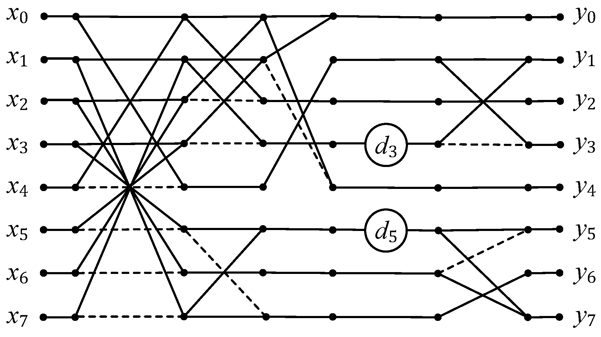
Figure 6 shows a data-flow diagram corresponding to the calculation of the output vector ${\mathbf{y}}_8$, where $d_3=cos{\varphi }_8$ and $d_5=sin{\varphi }_8$.

When the vector ${\mathbf{z}}_8={\mathbf{a}}_8+i{\mathbf{b}}_8$ of complex coefficients of DFT for the real input vector ${\mathbf{x}}_8$ is needed, it can be easily obtained from the output vector ${\mathbf{y}}_8$ of RDFT, according to (15)

$${\mathbf{a}}_8=\left[\begin{array}{c}{a}_0\\ a_1\\ a_2\\ a_3\\ a_4\\ a_5\\ a_6\\ a_7\end{array}\right]=\left[\begin{array}{c}{y}_0\\ y_1\\ y_2\\ y_3\\ y_4\\ y_3\\ y_2\\ y_1\end{array}\right]{\mathbf{b}}_8=\left[\begin{array}{c}{b}_0\\ b_1\\ b_2\\ b_3\\ b_4\\ b_5\\ b_6\\ b_7\end{array}\right]=\left[\begin{array}{c}0\\ -y_7\\ -y_6\\ -y_5\\ 0\\ y_5\\ y_6\\ y_7\end{array}\right]$$

(70)

The algorithm of the RDFT for $N=8$, presented in Figure 6, can be described by the following matrix–vector procedure, in which the matrix ${\mathbf{R}}_8$ has been factorized:

$${\mathbf{y}}_8={\mathbf{C}}_8{\mathbf{D}}_8{\tilde{\mathbf{A}}}_8{\overline{\mathbf{A}}}_8{\widehat{\mathbf{A}}}_8{\mathbf{x}}_8$$

(71)

where

$${\widehat{\mathbf{A}}}_8=\left[\begin{array}{cccccccc}1& 0& 0& 0& 1& 0& 0& 0\\ 0& 1& 0& 0& 0& 0& 0& 1\\ 0& 0& 1& 0& 0& 0& 1& 0\\ 0& 0& 0& 1& 0& 1& 0& 0\\ 1& 0& 0& 0& -1& 0& 0& 0\\ 0& 0& 0& 1& 0& -1& 0& 0\\ 0& 0& 1& 0& 0& 0& -1& 0\\ 0& 1& 0& 0& 0& 0& 0& -1\end{array}\right]{\overline{\mathbf{A}}}_8=\left[\begin{array}{cccccccc}1& 0& 1& 0& 0& 0& 0& 0\\ 0& 1& 0& 1& 0& 0& 0& 0\\ 1& 0& -1& 0& 0& 0& 0& 0\\ 0& 1& 0& -1& 0& 0& 0& 0\\ 0& 0& 0& 0& 1& 0& 0& 0\\ 0& 0& 0& 0& 0& 1& 0& 1\\ 0& 0& 0& 0& 0& 0& 1& 0\\ 0& 0& 0& 0& 0& -1& 0& 1\end{array}\right]$$

(72)

$${\tilde{\mathbf{A}}}_8=\left[\begin{array}{cccccccc}1& 1& 0& 0& 0& 0& 0& 0\\ 0& 0& 0& 0& 1& 0& 0& 0\\ 0& 0& 1& 0& 0& 0& 0& 0\\ 0& 0& 0& 1& 0& 0& 0& 0\\ 1& -1& 0& 0& 0& 0& 0& 0\\ 0& 0& 0& 0& 0& 1& 0& 0\\ 0& 0& 0& 0& 0& 0& 1& 0\\ 0& 0& 0& 0& 0& 0& 0& 1\end{array}\right]{\mathbf{D}}_8=\left[\begin{array}{cccccccc}1& 0& 0& 0& 0& 0& 0& 0\\ 0& 1& 0& 0& 0& 0& 0& 0\\ 0& 0& 1& 0& 0& 0& 0& 0\\ 0& 0& 0& d_3& 0& 0& 0& 0\\ 0& 0& 0& 0& 1& 0& 0& 0\\ 0& 0& 0& 0& 0& d_5& 0& 0\\ 0& 0& 0& 0& 0& 0& 1& 0\\ 0& 0& 0& 0& 0& 0& 0& 1\end{array}\right]$$

(73)

$${\mathbf{C}}_8=\left[\begin{array}{cccccccc}1& 0& 0& 0& 0& 0& 0& 0\\ 0& 1& 0& 1& 0& 0& 0& 0\\ 0& 0& 1& 0& 0& 0& 0& 0\\ 0& 1& 0& -1& 0& 0& 0& 0\\ 0& 0& 0& 0& 1& 0& 0& 0\\ 0& 0& 0& 0& 0& 1& -1& 0\\ 0& 0& 0& 0& 0& 0& 0& 1\\ 0& 0& 0& 0& 0& 1& 1& 0\end{array}\right]$$

(74)

According to this algorithm we need only 20 additions and 2 multiplications of real numbers to calculate the output vector ${\mathbf{y}}_8$.

9. RDFT Algorithm for $\mathit{N}=\mathbf{9}$

For $N=9$, the Equation (17) will take the form

$${\mathbf{y}}_9={\mathbf{R}}_9{\mathbf{x}}_9$$

(75)

where

$${\mathbf{R}}_9=\left[\begin{array}{ccc}1& {\mathbf{1}}_{1\times 4}& {\mathbf{1}}_{1\times 4}\\ {\mathbf{1}}_{4\times 1}& {\mathbf{A}}_4& {\mathbf{B}}_4\\ {\mathbf{0}}_{4\times 1}& {\mathbf{C}}_4& {\mathbf{D}}_4\end{array}\right]$$

(76)

and ${\mathbf{1}}_{n\times k}$, ${\mathbf{0}}_{n\times k}$ are n by k submatrices with all entries equal to 1 or 0, respectively. After applying the reduction formulas and taking advantage of the fact that $cos3{\varphi }_9=cos(6\pi /9)=-0.5$, the component submatrices can be written in the following forms:

$${\mathbf{A}}_4=\left[\begin{array}{cccc}cos{\varphi }_9& cos2{\varphi }_9& -0.5& cos4{\varphi }_9\\ cos2{\varphi }_9& cos4{\varphi }_9& -0.5& cos{\varphi }_9\\ -0.5& -0.5& 1& -0.5\\ cos4{\varphi }_9& cos{\varphi }_9& -0.5& cos2{\varphi }_9\end{array}\right]$$

(77)

$${\mathbf{B}}_4=\left[\begin{array}{cccc}cos4{\varphi }_9& -0.5& cos2{\varphi }_9& cos{\varphi }_9\\ cos{\varphi }_9& -0.5& cos4{\varphi }_9& cos2{\varphi }_9\\ -0.5& 1& -0.5& -0.5\\ cos2{\varphi }_9& -0.5& cos{\varphi }_9& cos4{\varphi }_9\end{array}\right]$$

(78)

$${\mathbf{C}}_4=\left[\begin{array}{cccc}sin4{\varphi }_9& -sin{\varphi }_9& sin3{\varphi }_9& -sin2{\varphi }_9\\ sin3{\varphi }_9& -sin3{\varphi }_9& 0& sin3{\varphi }_9\\ sin2{\varphi }_9& sin4{\varphi }_9& -sin3{\varphi }_9& -sin{\varphi }_9\\ sin{\varphi }_9& sin2{\varphi }_9& sin3{\varphi }_9& sin4{\varphi }_9\end{array}\right]$$

(79)

$${\mathbf{D}}_4=\left[\begin{array}{cccc}sin2{\varphi }_9& -sin3{\varphi }_9& sin{\varphi }_9& -sin4{\varphi }_9\\ -sin3{\varphi }_9& 0& sin3{\varphi }_9& -sin3{\varphi }_9\\ sin{\varphi }_9& sin3{\varphi }_9& -sin4{\varphi }_9& -sin2{\varphi }_9\\ -sin4{\varphi }_9& -sin3{\varphi }_9& -sin2{\varphi }_9& -sin{\varphi }_9\end{array}\right]$$

(80)

It is easy to see that the matrix ${\mathbf{B}}_4$ can be obtained from the matrix ${\mathbf{A}}_4$ by reversing the order of its columns, and the matrix ${\mathbf{D}}_4$ is the opposite matrix to the matrix obtained from ${\mathbf{C}}_4$ by reversing the order of its columns. When we calculate the product of the matrix ${\mathbf{R}}_9$ by the input vector ${\mathbf{x}}_9$ we obtain

$$\left[\begin{array}{c}{y}_0\\ y_1\\ y_2\\ y_3\\ y_4\\ y_5\\ y_6\\ y_7\\ y_8\end{array}\right]=\left[\begin{array}{c}[x_0+(x_3+x_6)]+[(x_1+x_8)+(x_2+x_7)+(x_4+x_5)]\\ [x_0-0.5(x_3+x_6)]+cos{\varphi }_9[(x_1+x_8)]+cos2{\varphi }_9\left[(x_2+x_7)\right]+cos4{\varphi }_9[(x_4+x_5)]\\ [x_0-0.5(x_3+x_6)]+cos2{\varphi }_9[(x_1+x_8)]+cos4{\varphi }_9\left[(x_2+x_7)\right]+cos{\varphi }_9[(x_4+x_5)]\\ [x_0+(x_3+x_6)]-0.5[(x_1+x_8)+(x_2+x_7)+(x_4+x_5)]\\ [x_0-0.5(x_3+x_6)]+cos4{\varphi }_9[(x_1+x_8)]+cos{\varphi }_9\left[(x_2+x_7)\right]+cos2{\varphi }_9[(x_4+x_5)]\\ sin3{\varphi }_9\left[(x_3-x_6)]-sin2{\varphi }_9[(x_4-x_5)\right]-sin{\varphi }_9\left[(x_2-x_7)\right]+sin4{\varphi }_9[(x_1-x_8)]\\ sin3{\varphi }_9[(x_4-x_5)-(x_2-x_7)+(x_1-x_8)]\\ -sin3{\varphi }_9\left[(x_3-x_6)]-sin{\varphi }_9[(x_4-x_5)\right]+sin4{\varphi }_9\left[(x_2-x_7)\right]+sin2{\varphi }_9[(x_1-x_8)]\\ sin3{\varphi }_9\left[(x_3-x_6)]+sin4{\varphi }_9[(x_4-x_5)\right]+sin2{\varphi }_9\left[(x_2-x_7)\right]+sin{\varphi }_9[(x_1-x_8)]\end{array}\right]$$

(81)

To better understand the construction of the RDFT algorithm for $N=9$, we will introduce the notations $t_1=x_1+x_8$, $t_2=x_2+x_7$, $t_3=x_3+x_6$, $t_4=x_4+x_5$, $t_5=x_4-x_5$, $t_6=x_3-x_6$, $t_7=x_2-x_7$, $t_8=x_1-x_8$ and consider the sub-blocks of the output vector ${\mathbf{y}}_8$. The first sub-block is

$$\left[\begin{array}{c}{y}_1\\ y_2\\ y_4\end{array}\right]=\left[\begin{array}{c}{x}_0-0.5t_3\\ x_0-0.5t_3\\ x_0-0.5t_3\end{array}\right]+\left[\begin{array}{ccc}cos{\varphi }_9& cos2{\varphi }_9& cos4{\varphi }_9\\ cos2{\varphi }_9& cos4{\varphi }_9& cos{\varphi }_9\\ cos4{\varphi }_9& cos{\varphi }_9& cos2{\varphi }_9\end{array}\right]\left[\begin{array}{c}{t}_1\\ t_2\\ t_4\end{array}\right]=$$

$$=\left[\begin{array}{c}{x}_0-0.5t_3\\ x_0-0.5t_3\\ x_0-0.5t_3\end{array}\right]+\left[\begin{array}{cccc}1& 1& 1& 0\\ 1& -1& 0& 1\\ 1& 0& -1& -1\end{array}\right]\left[\begin{array}{cccc}{d}_5& 0& 0& 0\\ 0& d_6& 0& 0\\ 0& 0& d_7& 0\\ 0& 0& 0& d_8\end{array}\right]\left[\begin{array}{ccc}1& 1& 1\\ 1& 0& -1\\ 0& 1& -1\\ -1& 1& 0\end{array}\right]\left[\begin{array}{c}{t}_1\\ t_2\\ t_4\end{array}\right]$$

(82)

where $d_5={\displaystyle \frac{1}{3}}(cos{\varphi }_9+cos2{\varphi }_9+cos4{\varphi }_9)$, $d_6={\displaystyle \frac{1}{3}}(2cos{\varphi }_9-cos2{\varphi }_9-cos4{\varphi }_9)$, $d_7={\displaystyle \frac{1}{3}}(-cos{\varphi }_9+2cos2{\varphi }_9-cos4{\varphi }_9)$, $d_8={\displaystyle \frac{1}{3}}(-cos{\varphi }_9-cos2{\varphi }_9+2cos3{\varphi }_9)$.

The second sub-block is

$$\left[\begin{array}{c}{y}_5\\ y_7\\ y_8\end{array}\right]=\left[\begin{array}{c}{t}_{4}sin3{\varphi }_9\\ -t_{4}sin3{\varphi }_9\\ t_{4}sin3{\varphi }_9\end{array}\right]+\left[\begin{array}{ccc}-sin2{\varphi }_9& -sin{\varphi }_9& sin4{\varphi }_9\\ -sin{\varphi }_9& sin4{\varphi }_9& sin2{\varphi }_9\\ sin4{\varphi }_9& sin2{\varphi }_9& sin{\varphi }_9\end{array}\right]\left[\begin{array}{c}{t}_5\\ t_7\\ t_8\end{array}\right]=$$

$$=\left[\begin{array}{c}{t}_{4}sin3{\varphi }_9\\ -t_{4}sin3{\varphi }_9\\ t_{4}sin3{\varphi }_9\end{array}\right]+\left[\begin{array}{cccc}1& 1& 1& 0\\ -1& 1& 0& -1\\ 1& 0& -1& -1\end{array}\right]\left[\begin{array}{cccc}{d}_9& 0& 0& 0\\ 0& d_{10}& 0& 0\\ 0& 0& d_{11}& 0\\ 0& 0& 0& d_{12}\end{array}\right]\left[\begin{array}{ccc}1& -1& 1\\ 1& 0& -1\\ 0& -1& -1\\ -1& -1& 0\end{array}\right]\left[\begin{array}{c}{t}_5\\ t_7\\ t_8\end{array}\right]$$

(83)

where $d_9={\displaystyle \frac{1}{3}}(sin{\varphi }_9-sin2{\varphi }_9+sin4{\varphi }_9)$, $d_{10}={\displaystyle \frac{1}{3}}(-sin{\varphi }_9-2sin2{\varphi }_9-sin4{\varphi }_9)$, $d_{11}={\displaystyle \frac{1}{3}}(2sin{\varphi }_9+sin2{\varphi }_9-sin4{\varphi }_9)$, $d_{12}={\displaystyle \frac{1}{3}}(-sin{\varphi }_9+sin2{\varphi }_9+2sin4{\varphi }_9)$.

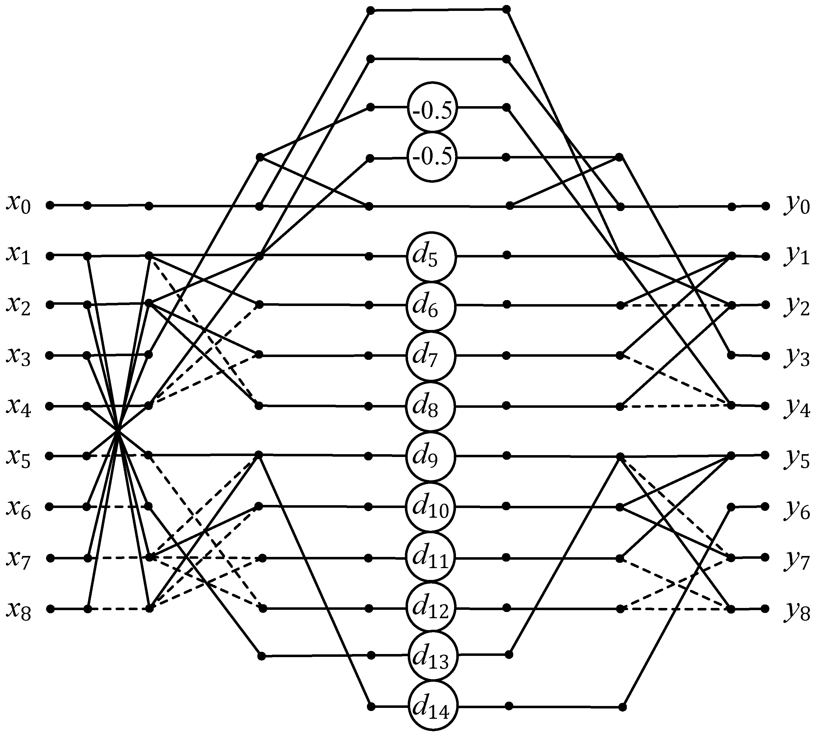
Figure 7 shows a data flow diagram corresponding to the calculation of the output vector ${\mathbf{y}}_9$, where $d_{13}=d_{14}=sin3{\varphi }_9$.

When the vector ${\mathbf{z}}_9={\mathbf{a}}_a+i{\mathbf{b}}_9$ of complex coefficients of DFT for the real input vector ${\mathbf{x}}_9$ is needed, it can be easily obtained from the output vector ${\mathbf{y}}_9$ of RDFT, according to (16)

$${\mathbf{a}}_9=\left[\begin{array}{c}{a}_0\\ a_1\\ a_2\\ a_3\\ a_4\\ a_5\\ a_6\\ a_7\\ a_8\end{array}\right]=\left[\begin{array}{c}{y}_0\\ y_1\\ y_2\\ y_3\\ y_4\\ y_4\\ y_3\\ y_2\\ y_1\end{array}\right]{\mathbf{b}}_7=\left[\begin{array}{c}{b}_0\\ b_1\\ b_2\\ b_3\\ b_4\\ b_5\\ b_6\\ b_7\\ b_8\end{array}\right]=\left[\begin{array}{c}0\\ -y_8\\ -y_7\\ -y_6\\ -y_5\\ y_5\\ y_6\\ y_7\\ y_8\end{array}\right]$$

(84)

The algorithm of the RDFT for $N=9$, presented in Figure 7, can be described by the following matrix–vector procedure, in which the matrix ${\mathbf{R}}_9$ has been factorized:

$${\mathbf{y}}_9={\mathbf{C}}_{9\times 11}{\tilde{\mathbf{C}}}_{11\times 15}{\mathbf{D}}_{15}{\tilde{\mathbf{A}}}_{15\times 11}{\overline{\mathbf{A}}}_{11\times 9}{\widehat{\mathbf{A}}}_9{\mathbf{x}}_9$$

(85)

where

$${\widehat{\mathbf{A}}}_9=\left[\begin{array}{ccccccccc}1& 0& 0& 0& 0& 0& 0& 0& 0\\ 0& 1& 0& 0& 0& 0& 0& 0& 1\\ 0& 0& 1& 0& 0& 0& 0& 1& 0\\ 0& 0& 0& 1& 0& 0& 1& 0& 0\\ 0& 0& 0& 0& 1& 1& 0& 0& 0\\ 0& 0& 0& 0& 1& -1& 0& 0& 0\\ 0& 0& 0& 1& 0& 0& -1& 0& 0\\ 0& 0& 1& 0& 0& 0& 0& -1& 0\\ 0& 1& 0& 0& 0& 0& 0& 0& -1\end{array}\right]$$

(86)

$${\overline{\mathbf{A}}}_{11\times 9}=\left[\begin{array}{ccccccccc}0& 0& 0& 1& 0& 0& 0& 0& 0\\ 1& 0& 0& 0& 0& 0& 0& 0& 0\\ 0& 1& 1& 0& 1& 0& 0& 0& 0\\ 0& 1& 0& 0& -1& 0& 0& 0& 0\\ 0& 0& 1& 0& -1& 0& 0& 0& 0\\ 0& -1& 1& 0& 0& 0& 0& 0& 0\\ 0& 0& 0& 0& 0& 1& 0& -1& 1\\ 0& 0& 0& 0& 0& 1& 0& 0& -1\\ 0& 0& 0& 0& 0& 0& 0& -1& -1\\ 0& 0& 0& 0& 0& -1& 0& -1& 0\\ 0& 0& 0& 0& 0& 0& 1& 0& 0\end{array}\right]$$

(87)

$${\tilde{\mathbf{A}}}_{15\times 11}=\left[\begin{array}{ccccccccccc}0& 1& 0& 0& 0& 0& 0& 0& 0& 0& 0\\ 0& 0& 1& 0& 0& 0& 0& 0& 0& 0& 0\\ 1& 0& 0& 0& 0& 0& 0& 0& 0& 0& 0\\ 0& 0& 1& 0& 0& 0& 0& 0& 0& 0& 0\\ 1& 1& 0& 0& 0& 0& 0& 0& 0& 0& 0\\ 0& 0& 1& 0& 0& 0& 0& 0& 0& 0& 0\\ 0& 0& 0& 1& 0& 0& 0& 0& 0& 0& 0\\ 0& 0& 0& 0& 1& 0& 0& 0& 0& 0& 0\\ 0& 0& 0& 0& 0& 1& 0& 0& 0& 0& 0\\ 0& 0& 0& 0& 0& 0& 1& 0& 0& 0& 0\\ 0& 0& 0& 0& 0& 0& 0& 1& 0& 0& 0\\ 0& 0& 0& 0& 0& 0& 0& 0& 1& 0& 0\\ 0& 0& 0& 0& 0& 0& 0& 0& 0& 1& 0\\ 0& 0& 0& 0& 0& 0& 0& 0& 0& 0& 1\\ 0& 0& 0& 0& 0& 0& 1& 0& 0& 0& 0\end{array}\right]$$

(88)

$${\mathbf{D}}_{15}=\left[\begin{array}{ccccccccccccccc}1& 0& 0& 0& 0& 0& 0& 0& 0& 0& 0& 0& 0& 0& 0\\ 0& 1& 0& 0& 0& 0& 0& 0& 0& 0& 0& 0& 0& 0& 0\\ 0& 0& -0.5& 0& 0& 0& 0& 0& 0& 0& 0& 0& 0& 0& 0\\ 0& 0& 0& -0.5& 0& 0& 0& 0& 0& 0& 0& 0& 0& 0& 0\\ 0& 0& 0& 0& 1& 0& 0& 0& 0& 0& 0& 0& 0& 0& 0\\ 0& 0& 0& 0& 0& d_5& 0& 0& 0& 0& 0& 0& 0& 0& 0\\ 0& 0& 0& 0& 0& 0& d_6& 0& 0& 0& 0& 0& 0& 0& 0\\ 0& 0& 0& 0& 0& 0& 0& d_7& 0& 0& 0& 0& 0& 0& 0\\ 0& 0& 0& 0& 0& 0& 0& 0& d_8& 0& 0& 0& 0& 0& 0\\ 0& 0& 0& 0& 0& 0& 0& 0& 0& d_9& 0& 0& 0& 0& 0\\ 0& 0& 0& 0& 0& 0& 0& 0& 0& 0& d_{10}& 0& 0& 0& 0\\ 0& 0& 0& 0& 0& 0& 0& 0& 0& 0& 0& d_{11}& 0& 0& 0\\ 0& 0& 0& 0& 0& 0& 0& 0& 0& 0& 0& 0& d_{12}& 0& 0\\ 0& 0& 0& 0& 0& 0& 0& 0& 0& 0& 0& 0& 0& d_{13}& 0\\ 0& 0& 0& 0& 0& 0& 0& 0& 0& 0& 0& 0& 0& 0& d_{14}\end{array}\right]$$

(89)

$${\tilde{\mathbf{C}}}_{11\times 15}=\left[\begin{array}{ccccccccccccccc}0& 0& 0& 1& 1& 0& 0& 0& 0& 0& 0& 0& 0& 0& 0\\ 1& 0& 0& 0& 1& 0& 0& 0& 0& 0& 0& 0& 0& 0& 0\\ 1& 0& 1& 0& 0& 1& 0& 0& 0& 0& 0& 0& 0& 0& 0\\ 0& 0& 0& 0& 0& 0& 1& 0& 0& 0& 0& 0& 0& 0& 0\\ 0& 0& 0& 0& 0& 0& 0& 1& 0& 0& 0& 0& 0& 0& 0\\ 0& 0& 0& 0& 0& 0& 0& 0& 1& 0& 0& 0& 0& 0& 0\\ 0& 0& 0& 0& 0& 0& 0& 0& 0& 1& 0& 0& 0& 1& 0\\ 0& 0& 0& 0& 0& 0& 0& 0& 0& 0& 1& 0& 0& 0& 0\\ 0& 0& 0& 0& 0& 0& 0& 0& 0& 0& 0& 1& 0& 0& 0\\ 0& 0& 0& 0& 0& 0& 0& 0& 0& 0& 0& 0& 1& 0& 0\\ 0& 0& 0& 0& 0& 0& 0& 0& 0& 0& 0& 0& 0& 0& 1\end{array}\right]$$

(90)

$${\mathbf{C}}_{9\times 11}=\left[\begin{array}{ccccccccccc}0& 1& 0& 0& 0& 0& 0& 0& 0& 0& 0\\ 0& 0& 1& 1& 1& 0& 0& 0& 0& 0& 0\\ 0& 0& 1& -1& 0& 1& 0& 0& 0& 0& 0\\ 1& 0& 0& 0& 0& 0& 0& 0& 0& 0& 0\\ 0& 0& 1& 0& -1& -1& 0& 0& 0& 0& 0\\ 0& 0& 0& 0& 0& 0& 1& 1& 1& 0& 0\\ 0& 0& 0& 0& 0& 0& 0& 0& 0& 0& 1\\ 0& 0& 0& 0& 0& 0& -1& 1& 0& -1& 0\\ 0& 0& 0& 0& 0& 0& 1& 0& -1& -1& 0\end{array}\right]$$

(91)

According to this algorithm, we need only 36 additions and 10 multiplications (and 2 shifts) of real numbers to calculate the output vector ${\mathbf{y}}_9$.

10. Discussion

Table 1. Comparison of the number of arithmetic operations for the proposed algorithms and Winograd’s algorithms described in [1].

N	Proposed Solution		Winograd’s Small-Lengths DFTs
	×	+	×	+
3	2	4	2	6
4	0	6	0	8
5	5	13	5	17
6	4	14	-	-
7	8	30	8	36
8	2	20	2	26
9	10	36	10	44

compares the number of multiplications (×) and additions (+) of real numbers necessary to determine the DFTs for real data vectors according to the proposed algorithms and Winograd’s algorithms designed specifically for small data lengths N. We compare our solutions with the corresponding Winograd’s algorithms because although these solutions are quite old they are the best in terms of multiplicative complexity. It should be remembered that the hardware multiplier is a very resource-intensive unit. The multiplier is the most resource-intensive and energy-consuming arithmetic unit, occupying a large area of the chip and dissipating a lot of power. Therefore, the use of complex and resource-intensive FPGAs containing a large number of multipliers without a special need is impractical. They use more power, take up more PCB space, and generate more heat than simpler chips. Thus, using less sophisticated chips and lower thermal management overheads translates into reduced processor size, weight, power consumption, and cost, as well as increased reliability as an added benefit.

The advantage of the presented Winograd-type algorithms in comparison with the Cooley–Tukey algorithms is that the critical path in the graph of any of the obtained algorithms contains only one multiplication. If there is more than one multiplication in the critical path of the algorithm, then this will create additional problems for the implementation of computations. As a result of multiplying two n-bit operands, a $2n$-bit product is obtained. The need for repeated multiplication requires an additional amount of manipulations with the operands and therefore requires more time and effort than when we are dealing with only a single multiplication.

It is easy to observe that the numbers of necessary multiplications are the same for the proposed algorithms as in Winograd’s algorithms, but the number of needed additions is smaller in the case of the solutions presented in the article. It must be said that the difference in the number of addition operations for the compared solutions is minimal and is not the main trump card of our paper. Our main goal was to reveal those aspects and features of the organization of calculations of small-size real-valued DFTs that were not disclosed in the available literature.

11. Conclusions

The paper presents a complete set of algorithms for real short-length RDFTs for N from 3 to 9. The corresponding signal flow graphs are also presented. The structure of each such graph, if necessary, can be directly mapped to the VLSI structure. The described algorithms are written in matrix–vector notation, where RDFT matrices are factorized and the factors are sparse matrices. This factorization reduces the number of arithmetic operations. Although the presented algorithms do not have a repeating structure for different lengths of input vectors, in some cases they may be more applicable and convenient in terms of implementation. One way or another, the solutions proposed by us are original and may be helpful. It should be emphasized that the diversity of existing approaches to the optimization of calculations cannot serve as an argument for stopping the search for new solutions, which may be more effective from the point of view of previously neglected criteria. Therefore, any rational approach to solving the current problem has the right to exist because each new look and each new solution of a known issue, which was previously solved by another method, stimulates the development of theory and practice, expands and deepens our knowledge in the relevant field of science or technology and, at least from this point of view, is helpful.

References

- Blahut, R.E. Fast Algorithms for Signal Processing; Cambridge University Press: New York, NY, USA, 2010. [Google Scholar]
- Pratt, W.K. Digital Image Processing; John Wiley and Sons, Inc.: New York, NY, USA, 1991. [Google Scholar]
- McClellan, J.H.; Rader, C.M. Number Theory in Digital Signal Processing; Prentice-Hall, Inc.: Englewood Cliffs, NJ, USA, 1979. [Google Scholar]
- Nussbaumer, H.J. Fast Fourier Transform and Convolution Algorithms; Springer: Berlin/Heidelberg, Germany, 1982. [Google Scholar]
- Burrus, S.; Parks, T.W.; Potts, J.F. DFT/FFT and Convolution: Algorithms and Implementation; John Wiley & Sons: New York, NY, USA, 1985. [Google Scholar]
- Garg, H.K. Digital Signal Processing Algorithms: Number Theory, Convolution, Fast Fourier Transforms, and Applications; CRC Press: Boca Raton, FL, USA, 1998. [Google Scholar]
- Bi, G.; Zeng, Y. Transforms and Fast Algorithms for Signal Analysis and Representations; Birkhäuser: Basel, Switzerland, 2004. [Google Scholar]
- Cooley, J.W.; Tukey, J.W. An algorithm for the machine calculation of complex Fourier series. Math. Comput. 1965, 19, 297–301. [Google Scholar] [CrossRef]
- Gold, B.; Rader, C.M. Digital Processing of Signals; McGraw-Hill: New York, NY, USA, 1969. [Google Scholar]
- Rabiner, L.R.; Gold, B. Theory and Application of Digital Signal Processing; Prentice Hall: Englewood Cliff, NJ, USA, 1975. [Google Scholar]
- Bogner, R.E.; Constantinides, A.G. Introduction to Digital Filtering; John Wiley & Sons: New York, NY, USA, 1975. [Google Scholar]
- Voronenko, Y.; Püschel, M. Algebraic Signal Processing Theory: Cooley-Tukey Type Algorithms for Real DFTs. IEEE Trans. Signal Process. 2009, 57, 205–222. [Google Scholar] [CrossRef]
- Martens, J.-B. Discrete Fourier transform algorithms for real valued sequences. IEEE Trans. ASSP 1984, 32, 390–396. [Google Scholar] [CrossRef]
- Hu, N.-C.; Ersoy, O.K. Fast computation of real discrete Fourier transform for any number of data points. IEEE Trans. Circuits Syst. 1991, 38, 1280–1292. [Google Scholar] [CrossRef]
- Murakami, H. Real-valued decimation-in-time and decimation-in-frequency algorithms. IEEE Trans. Circuits Syst. II Analog. Digit. Signal Process. 1994, 41, 808–816. [Google Scholar] [CrossRef]
- Murakami, H. Real-valued fast discrete Fourier transform and cyclic convolution algorithms of highly composite even length. In Proceedings of the 1996 IEEE International Conference on Acoustics, Speech, and Signal Processing Conference Proceedings, Atlanta, GA, USA, 9 May 1996; Volume 3, pp. 1311–1314. [Google Scholar]
- Sorensen, H.V.; Jones, D.L.; Heideman, M.T.; Burrus, C.S. A split-radix real-valued fast Fourier transform. In Proceedings of the 3rd European Signal Processing Conference, The Hague, The Netherlands, 2–5 September 1986; pp. 287–290. [Google Scholar]
- Sorensen, H.V.; Jones, D.L.; Heideman, M.T.; Burrus, C.S. Realvalued fast Fourier transform algorithms. IEEE Trans. ASSP 1987, 35, 849–863. [Google Scholar] [CrossRef] [Green Version]
- Uniyal, P.R. Transforming real-valued sequences: Fast Fourier versus fast Hartley transform algorithms. IEEE Trans. Signal Process. 1994, 42, 3249–3254. [Google Scholar] [CrossRef]
- Vernet, J.L. Real signals fast Fourier transform: Storage capacity and step number reduction by means of an odd discrete Fourier transform. Proc. IEEE 1971, 59, 1531–1532. [Google Scholar] [CrossRef]
- Heideman, M.T.; Burrus, C.S.; Johnson, H.W. Prime factor FFT algorithms for real-valued series. In Proceedings of the ICASSP’84—IEEE International Conference on Acoustics, Speech, and Signal Processing, San Diego, CA, USA, 19–21 March 1984; pp. 28A.7.1–28A.7.4. [Google Scholar]
- Bergland, G.D. A fast Fourier transform algorithm for real-valued series. Commun. ACM 1968, 11, 703–710. [Google Scholar] [CrossRef]
- Bergland, G.D. A radix-eight fast Fourier transform subroutine for real-valued series. IEEE Trans. Audio Electroacoust. 1969, 17, 138–144. [Google Scholar] [CrossRef]
- Kumaresan, R.; Gupta, P.K. A prime factor FFT algorithm with real valued arithmetic. Proc. IEEE 1985, 73, 1241–1243. [Google Scholar] [CrossRef]
- Ersoy, O.K. Real discrete Fourier transform. IEEE Tran. Acoust. Speech Signal Process. 1985, 33, 880–882. [Google Scholar] [CrossRef]
- Ersoy, O.K.; Hu, N.C. Fast algorithms for the real discrete Fourier transform. In Proceedings of the ICASSP-88, International Conference on Acoustics, Speech, and Signal Processing, New York, NY, USA, 11–14 April 1988; Volume 3, pp. 1902–1905. [Google Scholar]
- Sundararajan, D.; Ahmad, M.O.; Swamy, M.N.S. Fast computation of the discrete Fourier transform of real data. IEEE Trans. Signal Process. 1997, 45, 2010–2022. [Google Scholar] [CrossRef]
- Parsons, T.W. A Winograd-Fourier transform algorithm for real valued data. IEEE Trans. Acoust. Speech Signal Process. 1979, 27, 398–402. [Google Scholar] [CrossRef]
- Sekhar, B.R.; Prabhu, K.M.M. Radix-2 decimation in frequency algorithm for the computation of the real-valued FFT. IEEE Trans. Signal Process. 1999, 47, 1181–1184. [Google Scholar] [CrossRef]
- Yin, X.; Yu, F.; Ma, Z. Resource-efficient pipelined architectures for radix-2 real-valued FFT with real datapaths. IEEE Trans. Circuits Syst. II Express Briefs 2016, 63, 803–807. [Google Scholar] [CrossRef]
- Chi, H.-F.; Lai, Z.-H. A cost-effective memory-based real-valued FFT and Hermitian symmetric IFFT processor for DMT-based wire-line transmission systems. In Proceedings of the 2005 IEEE International Symposium on Circuits and Systems (ISCAS), Kobe, Japan, 23–26 May 2005; Volume 6, pp. 6006–6009. [Google Scholar]
- Garrido, M.; Parhi, K.K.; Grajal, J. A pipelined FFT architecture for real-valued signals. IEEE Trans. Circuits Syst. I Reg. Pap. 2009, 56, 2634–2643. [Google Scholar] [CrossRef] [Green Version]
- Ayinala, M.; Parhi, K.K. Parallel-pipelined radix-22 FFT architecture for real valued signals. In Proceedings of the 2010 Conference Record of the Forty Fourth Asilomar Conference on Signals, Systems and Computers, Pacific Grove, CA, USA, 7–10 November 2010; pp. 1274–1278. [Google Scholar]
- Ayinala, M.; Lao, Y.; Parhi, K.K. An in-place FFT architecture for real-valued signals. IEEE Trans. Circuits Syst. II Exp. Briefs 2013, 60, 652–656. [Google Scholar] [CrossRef]
- Ayinala, M.; Parhi, K.K. FFT architectures for real-valued signals based on radix- 23 and radix-24 algorithms. IEEE Trans. Circuits Syst. I Reg. Pap. 2013, 60, 2422–2430. [Google Scholar] [CrossRef]
- Salehi, S.A.; Amirfattahi, R.; Parhi, K.K. Pipelined architectures for real-valued FFT and Hermitian-symmetric IFFT with real datapaths. IEEE Trans. Circuits Syst. II Exp. Briefs 2013, 60, 507–511. [Google Scholar] [CrossRef]
- Lao, Y.; Parhi, K.K. Canonic composite length real-valued FFT. J. Signal Process. Syst. 2018, 90, 1401–1414. [Google Scholar] [CrossRef]
- Zode, P.; Thor, A.; Deshmukh, A.Y. Folded FFT architecture for real-valued signals based on radix-23 algorithm. In Proceedings of the 2014 2nd International Conference on Devices, Circuits and Systems (ICDCS), Coimbatore, India, 6–8 March 2014; pp. 1–4. [Google Scholar]
- Mao, X.B.; Ma, Z.G.; Yu, F.; Xing, Q.J. A continuous-flow memory-based architecture for real-valued FFT. IEEE Trans. Circuits Syst. II Express Briefs 2017, 64, 1352–1356. [Google Scholar] [CrossRef]
- Yuan, M.; Ma, Z.; Yu, F.; Xing, Q. A novel address scheme for continuous-flow parallel memory-based real-valued FFT processor. Electronics 2019, 8, 1042. [Google Scholar] [CrossRef] [Green Version]
- Wiechno, T.; Yatsymirskyy, M. Two-stage fast Fourier and Hartley transform of real data sequence. Prz. Elektrotech. 2010, 86, 41–43. [Google Scholar]
Figure 1.
Data-flow diagram of the RDFT algorithm for .
Figure 2.
Figure 3.
Figure 4.
Data flow diagram of the RDFT algorithm for .
Figure 5.
Figure 6.
Figure 7.
Data–flow diagram of the RDFT algorithm for .