Inline Defective Laser Weld Identification by Processing Thermal Image Sequences with Machine and Deep Learning Techniques

Abstract

The non-destructive testing methods offer great benefit in detecting and classifying the weld defects. Among these, infrared (IR) thermography stands out in the inspection, characterization, and analysis of the defects from the camera image sequences, particularly with the recent advent of deep learning. However, in IR, the defect classification becomes a cumbersome task because of the exposure to the inconsistent and unbalanced heat source, which requires additional supervision. In light of this, authors present a fully automated system capable of detecting defective welds according to the electrical resistance properties in the inline mode. The welding process is captured by an IR camera that generates a video sequence. A set of features extracted by such video feeds supervised machine learning and deep learning algorithms in order to build an industrial diagnostic framework for weld defect detection. The experimental study validates the aptitude of a customized convolutional neural network architecture to classify the malfunctioning weld joints with mean accuracy of 99% and median f1 score of 73% across five-fold cross validation on our locally acquired real world dataset. The outcome encourages the integration of thermographic-based quality control frameworks in all applications where fast and accurate recognition and safety assurance are crucial industrial requirements across the production line.

1. Introduction

Welding is a fabrication process of joining metals by melting and fusing the parts together using high heat and pressure [1]. This welding process is prone to several defects including burn, crack, lack of penetration, overlap, and porosity [2,3,4]. There exist numerous other factors that affect the weld quality during or before the weld process, comprising metal condition, welding instrument quality, immature welding setup, and electrode contact status, among others [5].

The laser welding process serves to structurally assemble the battery modules by coupling a large number of smaller battery cells, however it may impair material structure arrangement that determines a higher electrical resistance aimed at poor joint quality [6]. In a laser welding process, electrical resistance of the weld, among several others, is a parameter to be considered and be contained in an acceptable range. The reason for the aforementioned phenomena comes from the fact that batteries are connected using welds and the increasing temperature of welds increases energy loss. Joule’s law states that a higher energy dissipation occurs during current flow, with a reduced efficiency and higher failure rate and risk of damage.

The main parameters that can compromise welding quality are related to the laser beam (intensity, focus position), shielding gas used, material coupling (fixtures and clamps not perfectly positioned), or material properties and conditions (thickness, cleanliness, reflectivity) [7]. Some of these factors cannot be systematically avoided with the industrial line design and many others could appear during a specific process; therefore, having an inline quality check allows to rework the single defected welding and therefore avoid discarding the whole battery pack without affecting cycle time or manufacturing settings.

Several other factors can concur and affect the result during the welding process, and understanding these factors is fundamental. The industries require fast, accurate, and less expensive defect detection solutions. The traditional weld quality testing methods may include random and periodic destructive testing that require to cut the sample under study into half to examine the weld quality [8]. The destructive testing is a cumbersome exercise and destroys the specimen [9]. When dealing with defects related to the electrical properties of the weld, several time-consuming measurements are usually performed to check the electrical resistance of the weld in several points.

Non-destructive testing (NDT) methods encompass ultrasonic testing, X-ray tomography, and infrared (IR) thermography, among others [10,11]. The NDT has received tremendous attention in the intelligent manufacturing industry such as aeronautics, automobile, nuclear plants, and railway tracks due to high-precision testing and cost effectiveness [12,13]. Moreover, unlike destructive testing methods, the NDT solutions seldom affect the sample under examination [14].

Monitoring and keeping track of the weld defect during video analysis is a difficult task, which begs the question of artificial intelligence (AI)-driven quality evaluation of the materials. Numerous frameworks have been proposed where imaging modalities with the help of intelligent methods offer automatic evaluation of the weld quality and defect detection [15,16,17,18,19,20,21]. The recent development in the field of NDT of weld defects using traditional machine learning (ML) and deep learning (DL) architectures has spanned through performance analysis to classification and detection to semantic segmentation to process monitoring and many more [22,23,24,25,26,27].

Yang et al. proposed a multilevel-feature-input-based deep neural network (DNN) for multiclass mechanical defect classification (porosity, crack, etc.) [28] on radiographic images, where the hidden layers of the DNN extract 11 different geometric and intensity contrast features of background and weld defect that eventually reach the last hidden layer for defect class prediction. The authors improved the detection accuracy by incorporating the fine-tuning of a stacked autoencoder as pretrained network and achieved an accuracy of 91.4%.

A transfer-learning-based weld classification framework on texture and geometric features over the X-ray images is presented by Ajmi et al. [29] for classifying different types of defects such as the porosity and lack of penetration. Due to the small-scale data availability, the authors performed data augmentation and tested several pretrained architectures including AlexNet, VGG-16, VGG-19, ResNet-50, ResNet-101, and GoogLeNet. All the networks achieved impressive accuracy, with ResNet-50 and ResNet-101 being top performers with an accuracy equal to 100%.

A semantic-segmentation-based three-stage weld classification method using DL on radiographic images is proposed by Chang et al. [30] for visual defect classification including porosity and cracks. The first phase is concerned with the weld defect screening on radiographic images using deep belief network (DBN), the second phase is responsible for cylindrical projection of the defected parts to ease the segmentation, while the last stage employs the SegNet architecture for the segmentation task. The adopted network requires no preprocessing and reaches an accuracy of 98.6%.

The studies referred to above consider the classification of mechanical defects. In the present study, the authors focused on the analysis of weld joints used to connect different lithium-ion cells to build a battery pack for electric vehicles; in this specific application, it is crucial to ensure the quality, both in terms of mechanical and electrical properties, i.e., the electrical resistance of the weld joint. This electrical characteristic is usually measured manually. It is a laborious and time-consuming task that could not be serviceable in an industrial setup. Moreover, the mechanical defects are generally physical and visible so can be classified considering morphological and textural features, whereas the defective weld joints that carry resistance issues may not have any visible defects, thus the traditional diagnostic imaging methods cannot efficiently be used. In fact, static images taken after the weld do not contain enough information to detect an electrical defect, thus explaining the need for a different approach.

IR thermography uses a thermal camera to record continuous temperature distribution profiles of the weld area of interest. Real-time monitoring of the weld pool, weld defect diagnosis, weld geometry determination, and autocorrection of welding parameters (when coupled with soft computing) are only a few of the applications of IR thermography in metal welding. Thermographic images are the most used when the heating and the cooling dynamics of the weld acquired during the welding process can reveal anything important for the defect detection and/or classification. IR thermography has been used for different kinds of applications, such as to monitor and control the weld geometry [31,32], to detect defects as lack of penetration and estimate of depth of penetration [33], and to perform seam tracking, bead width control, and cooling rate control to ensure acceptable weld quality with artificial neural networks [34]. The thermographic images have largely been studied with DL architectures [35,36,37], since they provide a gold standard for NDT methods. As an example, deep architectures have been employed to detect cracks [38] and characterize defects in a carbon-fiber-reinforced plastic specimen [39,40] by automatically analyzing thermal images and videos. To the best of the authors’ knowledge, there are no studies that solve the presented problem with the specific setup; hence, a detailed introduction is required to understand the conceived approach.

In this study, according to the industrial requirements of the Comau^® S.p.A., the authors propose several automatic classification frameworks capable of detecting a defective laser weld based on the electrical properties, i.e., the electrical resistance. As reported above, the analyzed industrial task considers the welding of different lithium-ion cells to build a battery pack for electric vehicles.

The studied process concerns the welding of nickel-plated aluminum tabs representing the cell’s electrode and a copper busbar. Busbars are solid metal bars used to carry current and place in connection the different cells; their technical attributes make busbars ideal for some high-voltage connections in electric vehicles.

The diagnostic intelligent frameworks developed in this study are able to classify, in real time, a weld joint as either defective or good depending on electrical properties of welded joints. The processed data consist of a single sequence of thermographic images acquired with IR camera during the welding and the cooling processes. A large set of features were extracted from the IR image sequence, and different classifiers are proposed, trained, and cross-validated, also by following three proposed workflows characterized by different feature reduction and selection procedures. Finally, a study and discussion of the execution time of the training and inference procedures of all evaluated classifiers is also reported.

The remainder of the article is organized as follows: Section 2 describes the materials and methods used during the study; the outcomes of the experimental studies are provided and discussed in Section 3; finally, the conclusive remarks and future perspectives are presented in Section 4.

2. Materials and Methods

The section adds the particulars about the data acquisition setup that is shown in Figure 1, feature extraction process, employed ML techniques and DL architectures, the conceived validation workflows, and the statistics approaches for the performance comparisons. The overall flow diagram of the experimental study is illustrated in Figure 2.

2.1. Welding Process and Data Acquisition

The implemented and tested frameworks have been validated on a dataset acquired with an industrial system designed and developed by Comau^®. The materials to be welded consist of a nickel layer, i.e., the cell electrode, having a thickness equal to 0.3 mm on a copper busbar with a thickness of 3 mm. The length of the weld joint is equal to 40 mm. The welding system is composed of the following subsystems (see Figure 1A–C):

• A laser welding system (the Comau^® LYTHE) that focuses the beam through a 200 mm collimator, creating a spot size of 0.15 mm with a continuous laser power equal to 2000 W;
• A 6-axes industrial robot (the Comau^® NJ 220) that is used to move the laser head (fixed to the robot flange) at a constant speed of 200 mm/s;
• Two 256 × 320 px thermal cameras based on microbolometer technology Teledyne^® FLIR A35 (each camera can record only one weld with a frame rate equal to 30 Hz) that are mounted 100 mm far away from the welding surface in a fixed setup and oriented over the clamping unit in such a way they can frame the entire 40 mm length linear weld stitch with a spatial resolution equal to 0.08 mm/px.

The thermal camera acquisition lasts 3 s and its start is triggered by the robot controller one second before the beginning of the welding. The acquisition timing has been designed in order to capture the thermal state just before the welding, the welding process lasts 200 ms, and the cooling dynamic lasts less than 1.5 s.

Just after each thermal video acquisition, an expert technician manually analyzed the electrical properties of the weld in order to annotate it either as ‘defective’ or ‘good’. This manual process consisted of (a) performing three different electrical resistance measurements at the top, middle, and bottom sections along the weld (see Figure 1F) by using an high-precision milliohmmeter supporting the four-wire method, (b) considering the maximum value among the three electrical resistance measurements, and (c) annotating the weld as defective if the maximum value is above a certain threshold and good otherwise. Such electrical resistance threshold clearly depends on the specific application and the characteristics of the welded parts. In the presented study, considering the desired performances of the entire battery pack and after a careful testing campaign with battery pack manufactures, the threshold value has been set to $20\mathsf{\mu }\mathsf{\Omega }$.

The collected industrial dataset is composed of 2305 thermal image sequences, out of which 2194 belong to negative class (non-defective) and the remaining 111 sequences to the positive class (i.e., defective class). Having available a large amount of defected weld image sequences is essential for ML and for DL models to properly capture the underlying patterns in the data; however, generally, there are significantly fewer samples of defects than those of non-defects, which account for merely 5% of the total data, bringing an unbalanced dataset [30].

2.2. Feature Description

The authors proposed three different analyses setups that lead to different groups of features. The aim is to describe cooling dynamic following the welding process, which has intrinsic diagnostic properties. The phenomenon under study is synthetically described as transient, both in time and space domains, by means of real-valued features.

A welded joint is identified as ‘good’ (or ‘non-defective’) if internal material layers are held together in a stable manner, i.e., without inclusions or geometrical dislocations. The hypothesis is that the heat will dissipate irregularly due to inner cavities, resulting in an atypical signal appearance on the surface. The presence of this kind of defect would alter the surface temperature distribution, and can be inspected directly by evaluating the weld nugget size and shape. Furthermore, the time distribution of the surface temperature gathers significant information in the assessment of specimen resistance properties, since it regards cooling dynamic in response to laser heat excitation.

As a first step, a rectangular region of interest (RoI) of the weld has been extracted from all the acquired raw frames of the video images sequence. The position and the size, i.e., 20 × 300 pixels, of such RoI have been experimentally defined in order to analyze only the surface of the welding without considering the surface of other metallic parts such as the clamping unit (see Figure 1C). It is worth reporting that all the three analyses that are reported below consider this RoI as input. The top section of Figure 2 reports a schematic explanation of the feature extraction process.

2.2.1. Cooling Analysis

As a first step, each frame has been split into 20 adjacent regions (region’s size is equal to 20 × 15 pixels) to study the local cooling dynamic along heat excitation sliding direction over time. Successively, the average temperature among the region’s pixels has been computed for each region and for each time frame. The presented cooling analysis has been independently conducted for each region and considers the study of the one-dimensional curve composed of the average temperature values over time. The first value of this curve is the average temperature of the time frame whose average value was greater than 50% with respect to the previous time frame, whereas the last value corresponds to the average value of the last time frame. The cooling analysis section in Figure 2 aids understanding the process presented above.

During the welding process, a huge quantity of heat is stored locally to the joint and is released to the surrounding environment in the next phase. The way this heat is cumulated and exchanged is deeply related to the welding’s penetration and internal structure. Considering the Newton’s cooling law, the derivative of the heat exchange Q (Joule) transfer versus time, or in other words, the cooling rate, is set proportional to the temperature (°C or K) gradient between the specimen T and the environment $T_a$ through heat transfer coefficient $\alpha$ (W/m${}^2$) and the exposed surface A (m${}^2$).

$$\frac{\partial \left(Q\right)}{dt}=-\alpha A(T-T_a)$$

(1)

In Equation (1), which is applicable only for one-dimension heat transfer between body and environment and represents a good simplification of the studied process, the cooling transient in time is defined as amplitude peak and time extension ratio. The segmented signal was described by a sum of two exponentially decaying signals $(a·e^{-b·t}+c·e^{-d·t})$ by means of four parameters, i.e., a, b, c, d, that accounted for curve amplitude (temperature, (a, c)) and velocity damping scale (b, d). Temperature curve dynamic was derived by minimizing the fitting error of the real curve, selecting the best parameters with least square difference regression. To characterize the shape of the cooling curve, following the heat excitation, the following features were considered:

• Multiplicative (a, c) and dumping factors (b, d) for exponential signals.
• Triangle area and triangle side ratio defined considering peak temperature (triangle height) and time interval between maximum temperature and minimum temperature reaching (triangle base). See part A of Figure 2 for the graphical representation of the aforementioned features.
• Root mean squared error in fitting real curve with least square algorithm, which weights previously extracted features.

2.2.2. Image Analysis

Along with welding process, different time instants are characterized by different weld nuggets areas and pictorial contents due to non-uniform emissivity of the materials. Contour segmentation of the weld nuggets allows to further measure its space extension and shape, while pixel values inside nuggets are related to the reached temperature.

Analysis of this spatial heat distribution is involved since it contains diagnostic information correlated to weld quality with a high degree of confidence [41]. Defects under the surface, such as small holes, cracks, or impurities, alter heat surface distribution due to internal variation of thermal capacitance. Hence, an inconsistent temperature distribution pattern would be produced and easily recognized in an IR video map.

Considering the high temperature of the specimen under testing, the authors incorporated the image processing pipeline that aims to examine the extension and texture of the segmented areas. The 3D matrix has width and height determined by the cropped ROI and a fixed depth of 13 subsequent and equally distributed frames in time. The first out of 13 time frames is the one characterized by an ROI mean pixel value greater than 20% of the ROI mean pixel value at the previous time frame.The pipeline initiates with the binarization, considering a threshold value over the pixel. All the pixels characterized by a temperature value higher than 45 °C have been set to white (that will represent weld nugget), and the rest to black for surrounding background.

When the pixels are thresholded independently of all surrounding pixels, the extracted regions may generally be noisy and/or contain small black regions in the segmented foreground. To overcome this, a final morphological closing using a disk-shaped structuring element bearing the size of 3 is performed in order to remove background pixels or, equivalently, to fill the foreground. Thereafter, for the largest connected component found in each frame, the following features are considered:

• Area;
• Eccentricity of the ellipse that best approximates the weld nugget;
• Ellipse major axis;
• Ellipse minor axis;
• Variance of pixels included into the weld nugget’s bounding box which has width and height of the extracted shape;
• Standard deviation of pixels included into the weld nugget’s bounding box which has width and height of the extracted shape.

2.2.3. Video Analysis

The video analysis considers whole pictorial content of frames both in time and space, without leaving any relevant information unattended and accommodating the entire duration of the video. The considered features are the following, where the term global refers to the value considering all pixels in the RoI cropped region and extending to all sampling frames.

• Min: the global-minimum pixel value;
• Max: the global-maximum pixel value;
• Mean: the global arithmetic mean of all the pixel values;
• Variance of all the pixels;
• Standard deviation of all pixels.

2.3. Classifiers

In this work, the authors have tested both traditional ML techniques and more recent DL approaches. The classification with classic ML algorithms was performed employing support vector machine (SVM), as presented in Boser et al. [42], K-nearest neighbor (KNN), originally introduced by Fix et al. in [43], and decision tree (DT) architectures, whose introduction is by Quinlan et al. [44] in their standard implementation. Moreover, DL-based implementation has considered a CNN with a customized architecture taking conceived features as input and described in detail in the following paragraph. It is worth mentioning that three different implementations of the CNN have been tested: (1) a CNN trained for the classification task (CNN-C), (2) a CNN trained to estimate the electrical resistance by using a weighted loss function (CNN-W), (3) a CNN trained to estimate the electrical resistance by using a modified (extended) version of the weighted loss function (CNN-EW). It is important to remark that when the CNN is trained to estimate the electrical resistance, the binary classification is performed by comparing the estimated value with the threshold used to annotate the dataset (see Section 2).

The Custom Convolutional Neural Networks

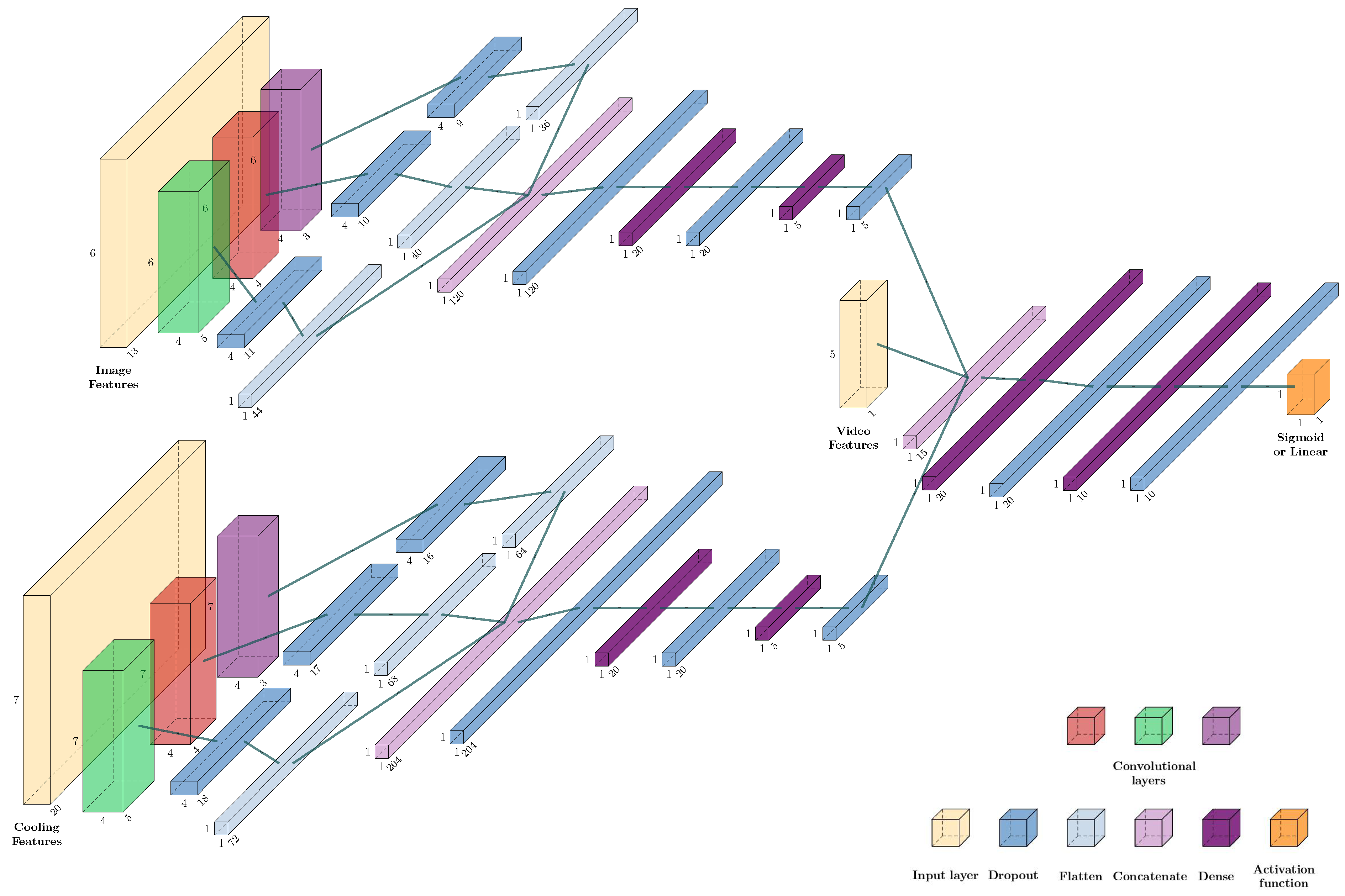
CNNs are well employed in DL frameworks, being able to sharpen pattern recognition ability inside customized kernels in a similar fashion as visual cortex does. In this study, the authors propose a hybrid CNN in which the convolutional layers and dense layers are stacked together for further representation learning, starting from 2D feature matrix as an input. It is worth mentioning that the CNN classification and regression are considered by implementing one and two different loss functions, respectively; however, the basic architecture of the CNN remains the same. The rationale for using a CNN that takes as input features is double: (I) the number of image sequences related to the defective welds is small to consider more complex topologies, and (II) the logical relation between the extracted features in time and space suggests the use of CNN filters.

The architecture provides, for parallel processing, two encoding paths for each feature matrix derived from cooling analysis and image analysis whose input layers can be denoted as $xϵ{\mathbb{R}}^{7\times 20}$ and ${\mathbb{R}}^{6\times 13}$ and a fully connected network branching from principal dense layers coming from convolutions, which keeps 1D video feature vector $ϵ$${\mathbb{R}}^{1\times 5}$. Each encoding path consists of the following:

• First layer, containing three convolutional layers, each of them has four bidimensional kernels, whose size are (7 × 3) for the first branch, (7 × 4) for the second, (7 × 5) for the third, processing for cooling feature matrix, and kernels of dimensions (6 × 3), (6 × 4), (6 × 5) for the image features matrix processing. These kernels are applied along feature matrix major dimension (see Figure 3 with stride 1, extracting information related to the spatial and temporal transients from adjacent regions and frames. The output of each filter has the first dimension flatten, the second determined by number of convolutions, and the third determined by number of applied convolutional filters: 1 × 18 × 4, 1 × 17 × 4, 1 × 16 × 4 and 1 × 11 × 4, 1 × 10 × 4, 1 × 9 × 4, respectively, for cooling feature matrix and image feature matrix. The activation function follows eLu exponential linear unit for classification oriented network and ReLu for regression ones (are both nonlinear activation functions).
• These outputs undergo dropout that selectively dumps number of neurons to prevent against vanishing gradient.
• Reshaped into a linear vector.
• Concatenate outputs in one linear vector bunching smaller ones coming from convolutional branches.
• Dropout stacked with 20 output dense neurons, followed by another dropout and five neuron-dense layers with hyperbolic tangent for classification task (CNN-C) and ReLu for regression task (CNN-W and CNN-EW).

The third input layer that consists of 1 × 5 video analysis features is connected with another two vectors of 1 × 5 dimension resulting from dropout layers of described parallel encoding paths. The last part of the network is set up by dropout and dense layers activated by hyperbolic tangent for classification and ReLu for regression, which gradually reduces flatten vector to one output value. The last layer of CNN performs sigmoid activation function in the CNN-C to predict class and linear activation function in the CNN-W and CNN-EW for the regression task.

For each acquired video, the proposed CNN has three separate input feature matrices, resulting from the segmentation in time and space domains of heating and cooling response dynamics (see Figure 2). In our real industrial scenario, the number of defective welds is extremely low, accounting for 5% of total amount of cases, thus explaining the need of a limited number of features. Controlling number of features by handcrafting them, even when feeding CNNs that have a priori ability to extract features by themselves, is motivated by the above-mentioned real-world conditions.

2.4. Workflows

In order to select the optimal feature set and abandon the irrelevant features, i.e., features having low or no contribution towards the classification, the authors exercised three different workflows elaborated in the section below: (i) considering pooled group of features, (ii) feature reduction capturing synthetic indicators of welding process distribution in time and space, (iii) feature selection following the previous step, stressing dimensionality reduction to drop possible redundant features, and leveraging classifiers’ learning ability to differently shape the phenomena under investigation. Extracted features are processed through proper classification algorithms and self-adjusted convolutional filters.

The three proposed pipelines include feature normalization according to interquartile range (IQR) of samples frequency distribution, in order to make the normalized values and the training phase more robust to the outliers that have not been removed. Equation (2) shows transformation adopted, where $\widehat{x}$ is the normalized value and $\overline{x}$ is the median.

$$\widehat{x}=\frac{x_i-\overline{x}}{IQR}$$

(2)

Workflow I, that follows a pooled group of features, employs both ML, i.e., DT, KNN, SVM, and DL, i.e., CNN, architectures, whereas the second and the third workflows only consider traditional ML models (see Figure 2 for schematic explanation). The CNN-based architectures have been trained and tested only within workflow I, because workflow II and workflow III consider too few features to justify a deep topology.

2.4.1. Workflow I: Pooled Group of Features

Workflow I accounts for evaluation of our basic hypothesis about phenomena description. It concerns the inclusion of 223 features derived from cooling analysis which places features in a 20 × 7 matrix, where each row contains the time transient curve parameters, the 13 × 6 matrix from image analysis, where each row contains morphological description of binarized weld nuggets, and the last five coming from video analysis, as previously described in the three cropped matrices presented in Figure 2.

2.4.2. Workflow II: Feature Reduction

The feature reduction aims to improve the generalization ability of the model. The process comprises the feature representation in a lower dimensionality space coming from the higher dimensions. In our implementation, high unbalancing against positive class can result in sparseness of data in consequence of the curse of dimensionality, which is about small number of observations in comparison to large numbers of variables.

In addition, precise description of the underlying dynamics, localizing features both in time and space, can lead to a learning burden for the classifiers. Moreover, it is desired for a classifier to be able to learn defect patterns independently from the precise localization among regions or frames. However, spatial and temporal connections were preserved because they characterize phenomena under study.

The proposed method reduces the cooling features for each of 20 adjacent regions and image analysis features for each of 13 frames considering minimum, mean, and maximum values to investigate usefulness of each nominal features defined on regions and frames rather than relying on punctual space and time features description.

Starting from 20 × 7 matrix, for each feature (i.e., dumping factor of exponential signal etc.), the minimum, mean, and maximum values across all regions are considered, reducing punctual representation among each of 20 regions in a summarized way; this leads to 7 × 3 matrix dimensions. The image analysis 13 × 6 starting matrix was reduced to 6 × 3 to account for the minimum, mean, and maximum values of each feature (i.e., area of thresholded image, etc.) encountered along time transients frames. The features regarding video analysis have not been reduced due to the fact that these values already refer to the globally extracted characteristics, so the total number consists of 44 features, describing the specimen response to laser heat welding excitation, both in time and space, but in a reduced way.

2.4.3. Workflow III: Feature Selection

The previous step might have introduced some similar or redundant features; therefore, the authors investigated the practicability of the feature selection. The feature informativeness was extracted through a recursive feature elimination (RFE) algorithm: an external estimator, in our case, KNN and DT classifiers, is responsible for assigning the weights to the feature. The job of RFE is to continuously repeat over tinier sets of features to select the optimal pool of features.

Initially, the training of the estimator is performed on the initial pool of features representing the second workflow, and the importance of each of these feature is obtained: for KNN classifier, those features are selected that give to the set number of neighbors, equal to 2, the faculty to include similar samples in the same homogeneous region; for DT classifier, the feature selection aims to minimize the expected surprise or entropy of the dataset, and ideally divide the samples in ’all good’ or ’all bad’ welds.

The features having less importance are pruned from the updated pool of features. The process keeps running until the desired number is achieved; in this study, it was set to 20.

2.5. Training of Classifiers

2.5.1. Cross-Validation

Data samples were divided into five stratified folds in which 80% and 20% were data subdivisions for the training and test sets, respectively. Every stratified fold presents the same relative frequency between positive and negative classes as that belonging to whole dataset. In order to make fair comparisons among the classifiers without biasing the results, the k-folds are the same for all the tested classifiers.

For ML classifiers, i.e., DT, KNN, and SVM, the best hyperparameters have been set with an exhaustive search over specified parameter values. The search consists of finding proper parameters related to the number of units processing information (tree nodes in DT), weighting observation related to a similarity measure (KNN), and constructing a separation hyperplane in feature dimension space exploiting kernel trick (SVM).

2.5.2. Decision Tree

The DT has a maximum depth of 20 leaf nodes, and a minimum number of samples in each leaf equal to 3 in order to avoid an extremely constrained tree and to prevent overfitting. The inner thresholds were set, minimizing the Gini information gain.

2.5.3. K-Nearest Neighbor

In the KNN algorithm, K represent the number of neighbors, which is the main actor for decision function. Optimization function in the KNN is convex, and allows existence of only one optimum point once the number of neighbors and distance metric are decided. It does not require training data for model generation.

In the majority voting, the class with the most votes among instant K-neighbors is held as prediction class and the vote is cast by each object to its respective class. For our data, the Euclidean distance finds closest similar points, and points are organized in nesting hyperspheres data structure. This not only results in cheap construction of the tree, as compared to the partition along the Cartesian axes, but also yields efficiency in high dimensions. A better stability was reached setting the value K = 2; in fact, for nearby values such as 1,3, and 4, the prediction showed a greater bias.

2.5.4. Support Vector Machine

The parameters were fine-tuned by grid searching a discrete space of combinations for kernel and C and gamma parameters. The decision function is built up, assigning to each sample a region of influence whose dimension is inversely related to gamma parameter. Moreover, C parameter trades off decision function’s compliance to training set with generalization ability. The grid search selected radial basis function (RBF) kernel, tuning C and gamma parameters. Gaussian kernel was selected in all three workflows, and a value for C = 200 and gamma = 0.005 was set to avoid overfitting. The parameter C is responsible for modulating the softness of the classification margin. The selection of the optimal parameter in the training data follows the highest cross-validation sensitivity for positive class.

2.5.5. CNNs

During the learning phase, the network stopping criterion is required by the CNN kernels. This stopping rule follows a certain point selection, i.e., number of epochs, learning curve surge or dip to a particular level, etc. Training updates the weights in order to tune the network’s input influence, hence optimizing the loss function. The network follows the stochastic gradient descent with momentum (SGDM) updating rule, where in this study the value of 0.7 is considered for momentum. The validation set checks the outcomes of the learning phase by computing the number of true positive samples, i.e., the ratio of correct positive classifications to the population of the validation set. The patience value denoted as P is set to 10 that early stops the learning process, which can reach a maximum of 1000 epochs, if recall decreases its value for 10 consecutive iterations on validation batches (i.e., acting as stopping criterion).

Training was reinitialized from scratch for each of the five learning folds, assigning CNN weights’ parameters following the He normal distribution. For instance, the DL approach commonly uses transfer learning from a pretrained network and uses it as a common starting point for fine-tuning to learn on a new similar task. In our specific case study, the CNN behaves as a ranking combining handcrafted features, learning to sharpen pattern perception.

2.5.6. Loss Function for the CNN-C

The unbalanced data result in uncertainty because, intrinsically, the binary classification models have equal probability for either class. Therefore, the class with more samples dominates and negatively influences the total loss [45]. On the other hand, the class with fewer samples fails to represent the target class, which requires comparable balanced data in order to reach unbiased outcomes.

This classification problem exhibits a large imbalance in the distribution of the target classes; for instance, there are many times more negative samples than the positive ones. Hence, the stratified sampling has been employed to ensure that relative class frequencies are approximately preserved in each train and test tests. The prediction function is learned using k-1 folds, and the fold left out is used for testing.

To counter this, the sigmoid focal loss function (originally introduced by Lin et al. [45]) has been adopted for object detection with high class unbalancing. The sigmoid focal loss function ignores the clearly classifiable examples and moves towards the so-called ’hard’ samples. It was found that balancing factor of 0.65 and modulating factor of 1.3 improved training stability in this case of heavy class imbalance.

2.5.7. Loss Functions for CNN-W and CNN-EW

Weighted sum of absolute error loss for CNN. The unbalancing between positive and negative number of samples accounts for around 1:19, respectively. This means that loss function has to recover to the high probability to see a negative sample and thus to avoid learning much more about this class. For this reason, the weighting factor $w_1$ has been introduced for positive class and $w_0$ for negative class that balances error on positive class roughly 19 times with respect to the error when true class is negative, multiplied to the absolute error between true and predicted resistance values. It can be argued that this solution does not consider whether the error is a false positive or a false negative.

$$w_1=\frac{NumberofPopulationSamples}{2\ast NumberofPositives}$$

(3)

$$w_0=\frac{NumberofPopulationSamples}{2\ast NumberofNegatives}$$

(4)

$$e=|Y-\widehat{Y}|$$

(5)

$$Erro{r}_i=\left\{\begin{array}{cc}e\ast w_1,\hfill & \mathrm{if}Y>20\hfill \\ e\ast w_0,\hfill & \mathrm{if}Y\le 20\hfill \end{array}\right.$$

$$WeightedSAELoss=\sum _{i=1}^{N}Erro{r}_i$$

(6)

In Equations (3) and (4), the digit 2 represents the number of classes, and in Equation (5), the parameter e is the absolute difference between true (Y) and predicted ($\widehat{Y}$) resistance values.

Extended weighted sum of absolute error loss for CNN. The extended weighted loss modifies the previous, penalizing false positive and false negative twice more. In case of true positive or true negative class recognized (after inverse transforming predictions and ground truth values, since they were normalized as mentioned in Section 2.4), error is considered to guide prediction layer to lower mean squared error (MSE) on resistance prediction. MSE is a metric monitoring overall performance of CNN regression during training. The mathematical explanation is provided in the following piecewise definition, where $FN,TP,FP,$ and $TN$ symbolize false negative, true positive, false positive, and true negative, respectively.

$$Erro{r}_i=\left\{\begin{array}{cc}e\ast w_1\ast 2,\hfill & \mathrm{if}Y>20\&\widehat{Y}\le 20forFN\hfill \\ e\ast w_1,\hfill & \mathrm{if}Y>20\&\widehat{Y}>20forTP\hfill \\ e\ast w_0\ast 2,\hfill & \mathrm{if}Y\le 20\&\widehat{Y}>20forFP\hfill \\ e\ast w_0,\hfill & \mathrm{if}Y\le 20\&\widehat{Y}\le 20forTN\hfill \end{array}\right.$$

$$ExtendedWeightedSAELoss=\sum _{i=1}^{N}Erro{r}_i$$

(7)

In both regression implementations, the total loss value accounted for the sum of absolute errors (SAE) reported on the batch data; see Equations (6) and (7).

2.6. Performance Criterion

Single performance criterion may not describe a classifier’s performance completely. Results become more reliable by increasing the number of evaluated performance criterion. Therefore, the authors used three performance-measuring metrics, precision, recall, and f1 score, for each class and global accuracy between classifiers. The selected performance metrics have been computed for each testing fold to obtain a distribution of confidence interval for each metric.

2.7. Comparisons and Statistics

This section illustrates the working guidelines used for the result evaluation in the study. Result presentation of the classification performance was followed by a between-classifiers comparative analysis including significance of the highlighted trends about both the negative and positive class.

Which classifier performs best for understanding the quality of the laser beam welds? It order to answer this question statistically, in the first instance, the performance of each classifier among its competitors trained on the same workflow is considered. This allowed to highlight best performances in terms of precision, recall, and f1 score on the same features; subsequently, for each metric distribution, all the classifiers’ performances have been compared among all workflows in order to evaluate which classifier (trained on a particular workflow) stands out with respect to other implementations and how it ranks when compared with other workflows and classifiers combinations.

In order to compare the classification scores, the performances have been computed on equal test sets obtained by using a five-fold cross validation with stratified splitting. The dependent variable is the overall score (for each metric on five-folds) and this is recorded in a separate variable for each method and for each workflow. This gives the possibility to derive an estimate of underlying performance distribution.

The hypothesis of Gaussian distribution does not hold due to the limited number of tests, so nonparametric Friedman test was chosen.

Nonparametric Friedman test and the Dunn’s pairwise post hoc tests with Bonferroni correction were carried out using medians to compare the scores for the different methods and workflows, to automatically check if pairwise comparisons were statistically significant once the main test was found globally consistent. In fact, Friedman first states the differences in terms of ranks between each pair of groups tested, and only if, once adjusted, p-values are less than statistical significance level, it allows for pairwise comparisons. The significance level was set to 0.05 and all the analyses were performed using the SPSS software (SPSS Inc., Chicago, IL, USA) Version 21.

3. Results And Discussion

The summarized experimental outcomes of the conceived classification pipelines in terms of mean accuracy, precision, recall, and f1 score, both for positive and negative classes, are listed in

Table 1. The experimental outcome of the workflow I using all employed techniques. CNN-C stands for CNN with classification implementation, the W and EW with network name indicate the weighted SAE and extended weighted SAE regression, respectively. Pos and Neg represent the positive and the negative classes.

Architecture	Accuracy	Precision		Recall		F1 Score
		Pos Class	Neg Class	Pos Class	Neg Class	Pos Class	Neg Class
DT	0.96 ± 0.01	0.62 ± 0.16	0.98 ± 0.01	0.55 ± 0.03	0.98 ± 0.01	0.57 ± 0.07	0.98 ± 0.01
KNN	0.97 ± 0.01	0.71 ± 0.07	0.98 ± 0.01	0.63 ± 0.07	0.99 ± 0.01	0.66 ± 0.04	0.98 ± 0.01
SVM	0.97 ± 0.01	0.70 ± 0.09	0.98 ± 0.01	0.52 ± 0.14	0.99 ± 0.06	0.58 ± 0.16	0.98 ± 0.01
CNN-C	0.99 ± 0.01	0.82 ± 0.09	0.98 ± 0.01	0.67 ± 0.03	0.99 ± 0.01	0.73 ± 0.03	0.99 ± 0.01
CNN-W	0.98 ± 0.01	0.41 ± 0.08	0.98 ± 0.01	0.69 ± 0.05	0.97 ± 0.01	0.51 ± 0.06	0.98 ± 0.01
CNN-EW	0.98 ± 0.01	0.45 ± 0.03	0.98 ± 0.01	0.67 ± 0.09	0.97 ± 0.01	0.54 ± 0.03	0.98 ± 0.01

,

Table 2. The experimental outcome of workflow II using all employed techniques. Pos and Neg represent the positive and the negative classes, respectively.

Architecture	Accuracy	Precision		Recall		F1 Score
		Pos Class	Neg Class	Pos Class	Neg Class	Pos Class	Neg Class
DT	0.96 ± 0.01	0.58 ± 0.10	0.98 ± 0.01	0.57 ± 0.13	0.98 ± 0.01	0.57 ± 0.11	0.98 ± 0.02
KNN	0.97 ± 0.01	0.67 ± 0.07	0.98 ± 0.01	0.58 ± 0.08	0.98 ± 0.01	0.62 ± 0.05	0.98 ± 0.01
SVM	0.98 ± 0.01	0.78 ± 0.08	0.98 ± 0.01	0.63 ± 0.05	0.99 ± 0.01	0.69 ± 0.05	0.99 ± 0.01

and

Table 3. The experimental outcome of workflow III using all employed techniques. Pos and Neg represent the positive and the negative classes, respectively.

Architecture	Accuracy	Precision		Recall		F1 Score
		Pos Class	Neg Class	Pos Class	Neg Class	Pos Class	Neg Class
DT	0.96 ± 0.01	0.65 ± 0.13	0.98 ± 0.01	0.56 ± 0.08	0.98 ± 0.01	0.60 ± 0.09	0.98 ± 0.01
KNN	0.96 ± 0.01	0.66 ± 0.06	0.98 ± 0.01	0.62 ± 0.04	0.98 ± 0.01	0.64 ± 0.04	0.98 ± 0.01
SVM	0.98 ± 0.01	0.70 ± 0.06	0.98 ± 0.01	0.60 ± 0.09	0.99 ± 0.01	0.65 ± 0.04	0.99 ± 0.01

. The precision, recall, and f1 score for the positive class are also pictorially depicted in the boxplots in Figure 4, Figure 5 and Figure 6.

It can be observed from Table 1, Table 2 and Table 3 that the negative class is always well interpreted among classifiers across the workflows due to large amount of available data for negative class, leading to a global accuracy range between 96% to 99%.

3.1. Workflow I Results

In the case of workflow I, the CNN architecture with the classification output layer outperforms in terms of precision and f1 score considering the positive class reaching 0.82 and 0.73, respectively. The KNN and SVM are significantly behind with respect to the precision of 0.71 and 0.70, respectively, while CNN weighted regression yields better recall, however, being less precise than CNN classification.

Conversely, SVM and DT are the worst-performing models in terms of recall in our experimental setup, achieving 0.52 and 0.55, respectively.

In our data for workflow I, statistically significant difference (p = 0.003) was found between CNN classification and CNN weighted regression, and with p = 0.003 between CNN classification and CNN extended weighted regression precision. Recall distribution of the CNN regression was statistically different from DT one (p = 0.035). The f1 score, which is harmonic mean between precision and recall, was stated different between CNN classification and both CNN regression; in particular, with a p = 0.006, CNN classification score was higher than CNN weighted regression and with p = 0.035, higher than CNN extended weighted regression.

3.2. Workflow II Results

The second feature setup, named workflow II, highlights the SVM’s capability in better subdividing dataspace when dimensionality reduction is performed, beating its previously acquired results in workflow I and its competitors in workflow II.

The DT offers the least stability with the largest standard deviation, however, with a nominal improvement in the recall value with respect to the previous setups.

Feature-reduction-training-based classifiers led to differences only in precision, stating superior scores of SVM with respect to the DT (p = 0.008). Instead, Friedman tests on recall and f1 score give p = 0.504 and p = 0.074, respectively.

3.3. Workflow III Results

Workflow III enhances DT performance regarding precision and f1 score, lowering the recall and flattening the performance of KNN, which yields best recall value.

In the feature selection (i.e., third) workflow, all classifiers do not yield statistically significant differences. Regarding precision, the Friedman analysis gives p = 0.449, for recall p = 0.472, and for f1 score p = 0.074.

3.4. One Versus All Results

In a second stage, the authors performed a more exhaustive comparison to select the combination of classifier and features on which learning gives best results. The number of comparisons tested simultaneously increased along with likelihood of erroneous inferences, thus requiring a more strict significance threshold. Regarding precision, it was found that between multiple comparisons, there were differences with a p < 0.000001. This allowed us to further inspect pairwise relationships: in particular, the CNN classification has a mean rank greater than CNN extended weighted regression and CNN weighted regression with an equal p = 0.001. SVM on workflow II ranked in the middle, with performance being greater than CNN extended weighted regression with p = 0.025 and with respect to CNN weighted regression with p = 0.018.

Friedman test on recall or sensitivity to positive cases does not reveal statistically different pairwise comparisons among classifiers and workflows with p = 0.304, but the three CNN implementations rank best. Statistical analysis regarding f1 score states the dominance of the CNN with classification layers on CNN extended weighted regression with p = 0.025 and on CNN weighted regression with p = 0.013.

The Friedman test does not reveal any statistically significant comparison among performance distribution about negative class, yielding p = 1.0 in each performed analysis.

Summing up, CNN with classification output layer performed best in both precision and f1 score with respect to other implementations, learning from the pooled group of features (see the Table 1). In fact, it can be stated that CNN with classification layer and trained on handcrafted features performed best among classifiers across the workflows, both regarding precision and f1 score for positive class. Thus, the initial hypothesis is fulfilled. In addition, feature reduction workflow has shed light on the ability of the SVM architecture to benefit from suppression of an amount of irrelevant features in the data samples.

3.5. Training and Inference Times

Thermographic videos and raw frames were processed by computational unit hardware Intel(R) Xenon(R) CPU E5-1620 [email protected] GHz with 16 GB RAM for the feature extraction process, training of ML classifiers, and parameters tuning, while DL architectures were trained on graphic card NVIDIA Quadro P4000, using Tensorflow and Sklearn Python 3.10 packages. In addition, the same hardware was used for test of trained networks. Reported results in

Table 4. Average and standard deviation training time measured in milliseconds taken by classifiers and respective workflows to shape decision function in five-fold learning sets.

Architecture	Training Time [ms]
	Workflow I	Workflow II	Workflow III
DT	462.01 ± 50.12	62.3 ± 6.10	21.60 ± 1.60
KNN	31.00 ± 0.44	6.41 ± 0.13	3.08 ± 0.42
SVM	15,133.05 ± 3535.01	304.33 ± 13.42	751.71 ± 270.14
CNN-C	60,490.02 ± 4856.31	-	-
CNN-W	271,991.80 ± 4456.70	-	-
CNN-EW	263,880.00 ± 4099.30	-	-

and

Table 5. Average and standard deviation time in milliseconds elapsed for single sample inference belonging to five-fold testing sets during prediction phase performed by classification methods and workflows illustrated. Measurements confirm the feasibility of inline testing and real-time quality assessment.

Architecture	Inference Time [ms]
	Workflow I	Workflow II	Workflow III
DT	0.27 ± 0.01	2.46 ± 0.37	0.21 ± 0.13
KNN	2.21 ± 0.32	1.53 ± 0.75	1.24 ± 0.25
SVM	0.36 ± 0.01	0.33 ± 0.01	0.03 ± 0.06
CNN-C	100.50 ± 5.20	-	-
CNN-W	61.60 ± 22.13	-	-
CNN-EW	48.03 ± 1.80	-	-

account for all classifiers and workflows combinations, whose performances were analyzed in Section 3. In the following table, training time refers to average time and standard deviation, measured in milliseconds, taken by classifiers to shape decision function in five-fold learning sets.

Table 4 shows that the DL architecture requires, on average, less than 5 min for learning phase, while ML algorithms take less than half of a minute. Feature reduction and feature selection have light-weighted model representation with an improved training convergence speed with respect to workflow I. The highlighted trend does not cover SVM; in fact, training time required reaches maximum value in workflow III. This is attributable to the high regularization, through setting C parameter, that constrained to converge to simple decision function, maintaining generalization ability on defective class. DT and KNN show monotonic decrease of the training duration as dimensionality is reduced, accompanied, for DT, by continuous increasing in precision, recall, and f1 score while KNN reaches best precision in workflow III with lowest learning time, with stable and slightly decreasing recall and f1 score, respectively. The SVM shows better performances regarding all three metrics from workflow I to workflow II, accompanied by five-times-reduced training time; however, SVM does not benefit from feature selection with increased learning time and reduced performances.

The DL classifiers require greater execution time than ML ones due to higher number of parameters; CNN-C is built on eLu and sigmoid activation functions that, combined with focal loss, yield to the fastest learning among CNNs.

Inference time reported in Table 5 refers to the average and standard deviation, measured in milliseconds, of time required to classify a single sample as ’defective’ or ’non-defective’ weld. ML classifiers, except DT, show a monotonic decreasing in inference time required, along with feature reduction and selection, that can be attributable to simple representation and mapping of samples. In addition, DL classifiers need less than a few hundred milliseconds with a minimal standard deviation. In absolute term, the elected method identified in CNN-C performs prediction in roughly 0.1 s.

Moreover, time required for feature extraction pipeline was measured and accounted for average value of 325.40 ms ± 26.71 ms; considering having trained the model, the whole time required from acquisition to classification step is roughly equal to 425.40 ms ± 30.00 ms, rounded to 0.5 s.

All implemented methods have inference time on a single data sample coherent with the industrial real-time requirements of fast anomaly detection without need to interrupt assembly lines.

4. Conclusions

This paper presented a machine and deep learning-based evaluation framework as a support in decision-making in industrial environment to detect defective weld joints according the electrical properties using thermographic image sequences acquired from IR camera recorded videos. The authors compared inference ability of different classifiers in combination with three different feature groups, fostering precision, recall, and f1 score on the positive class as key merit factors. The proposed adaption in the CNN with classification layer yields good results in the prediction of the weld resistance defects with high accuracy, precision, and f1 score. It was demonstrated that this implementation allows inline and real-time labeling of rare cases of defective welds that subsequently undergo repair or rewelding before the final assembly, thus avoiding the propagation of defects and improving efficiency. Additionally, the quality assurance of the metal products plays a pivotal role in satisfying customer quality specifications. From a manufacturer’s standpoint, the authors have further demonstrated the feasibility of inline anomaly detection systems to continually improve production methods.