
Adaptive Salp Swarm Algorithm for Optimization of Geotechnical Structures
by
 , , and
Mohammad Khajehzadeh
1 ,
,
Amin Iraji
2,*, 
Ali Majdi
3,
Suraparb Keawsawasvong
4 and
and
Moncef L. Nehdi
5,*
1
Department of Civil Engineering, Anar Branch, Islamic Azad University, Anar 77419-43615, Iran
2
Engineering Faculty of Khoy, Urmia University of Technology, Urmia 57166-93188, Iran
3
Department of Building and Construction Techniques, Al-Mustaqbal University College, Hillah 51001, Iraq
4
Department of Civil Engineering, Thammasat School of Engineering, Thammasat University, Bangkok 10200, Thailand
5
Department of Civil Engineering, McMaster University, Hamilton, ON L8S 4M6, Canada
*
Authors to whom correspondence should be addressed.
Appl. Sci. 2022, 12(13), 6749; https://doi.org/10.3390/app12136749
Submission received: 23 April 2022
/
Revised: 20 June 2022
/
Accepted: 28 June 2022
/
Published: 3 July 2022
(This article belongs to the Special Issue Novel Hybrid Intelligence Techniques in Engineering)
Abstract
:Based on the salp swarm algorithm (SSA), this paper proposes an efficient metaheuristic algorithm for solving global optimization problems and optimizing two commonly encountered geotechnical engineering structures: reinforced concrete cantilever retaining walls and shallow spread foundations. Two new equations for the leader- and followers-position-updating procedures were introduced in the proposed adaptive salp swarm optimization (ASSA). This change improved the algorithm’s exploration capabilities while preventing it from converging prematurely. Benchmark test functions were used to confirm the proposed algorithm’s performance, and the results were compared to the SSA and other effective optimization algorithms. A Wilcoxon’s rank sum test was performed to evaluate the pairwise statistical performances of the algorithms, and it indicated the significant superiority of the ASSA. The new algorithm can also be used to optimize low-cost retaining walls and foundations. In the analysis and design procedures, both geotechnical and structural limit states were used. Two case studies of retaining walls and spread foundations were solved using the proposed methodology. According to the simulation results, ASSA outperforms alternative models and demonstrates the ability to produce better optimal solutions.
1. Introduction
The objective function in most engineering problems is non-convex and discontinuous, with a large number of design variables. As a result, traditional deterministic optimization techniques based on mathematical principles may struggle to find a global optimum solution due to local optima trapping. The use of powerful metaheuristic optimization algorithms for obtaining a global optimum to overcome this limitation is of interest, and metaheuristic algorithms have proven to be an excellent alternative for solving complex problems in recent decades [1,2,3,4,5,6].
The most common geo-structures in practical application are reinforced concrete retaining walls and spread footings, which have received considerable attention in recent studies [7,8]. These structures are commonly used and typically involve a large volume of material. In the past, the initial anticipated dimensions of retaining structures were tested for stability and other building code requirements. If the dimensions were insufficient to meet the constraints, they were adjusted until all the requirements were met. During this time-consuming, iterative process, the cost of construction was not taken into account. In the optimum design of these structures, the dimensions that provide the lowest cost and weight of construction while meeting all the design requirements are automatically determined.
Several metaheuristic algorithms for geotechnical engineering problems have recently been developed and are widely used. Despite the fact that metaheuristic methods can produce acceptable results, no algorithm outperforms another in solving all the optimization problems. Furthermore, the objective function in most geotechnical engineering optimization problems, such as shallow foundations, retaining structures, and pile optimization, is discontinuous and has a large number of design variables. As a result, several research projects have been launched in order to improve the performance and efficiency of the existing metaheuristics. Some of these are modified particle swarm optimizations [9,10], modified harmony search algorithms [11], modified gravitational search algorithms [12], modified sine cosine algorithms [13], improved salp swarm algorithms [14], modified ant colony optimizations [15], modified teaching–learning-based optimizations [16], improved tunicate swarm algorithms [17], and modified wild horse optimizations [18]. According to the effectiveness of the metaheuristics and their modified versions, these methods have been widely used to solve several geotechnical engineering problems, as presented in Table 1.
A new meta-heuristic algorithm called the salp swarm algorithm (SSA) simulates salp fish swarming in deep waters [49]. Section 2 contains more information on the SSA’s motivation and mathematical modelling. The SSA in its basic model can be extended or hybridized with another algorithm to produce better answers for future problems, similar to other metaheuristic approaches [14,43,50].
This paper presents an adaptive salp swarm algorithm (ASSA) for optimization by introducing new position-updating equations for leader and follower salps. This change significantly improves the algorithm’s performance and convergence speed. A set of well-known standard benchmark functions from the literature is used to validate the effectiveness of the proposed approach. Furthermore, numerical geotechnical structure optimization tests are used to investigate the proposed method’s performance and efficiency.
2. Salp Swarm Algorithm
A salp is a type of marine animal in the Salpidae family. It has a cylindrical structure with apertures at the ends similar to those of a jellyfish, which move and eat by pumping water through internal feeding filters in their gelatinous bodies. The salp swarm algorithm (SSA), a population-based optimization technique, was developed by Mirjalili et al. [49]. The salp chain can be used to calculate the SSA’s behavior while hunting for optimal feeding sources (i.e., the target of this swarm is a food position in the search space called FP). To mathematically model salp chains, they are sampled into two groups: followers and leaders. The salp at the head of the chain is known as the leader, while the others are known as followers. The swarm is led by the leader of these salps, and the followers follow in his footsteps. The chain begins with a leader, who is followed by the followers to guide their movements.
Similar to other swarm-based algorithms, the salp location is specified in a n-dimensional search space, where n is the number of variables in a given problem. As a result, the positions of all the salps are recorded in a two-dimensional matrix known as X, as shown in Equation (1):
The fitness of each salp is then determined in order to define which salp has the best fitness. It is also supposed that the swarm’s goal is a food position called FP in the search area.
The following equation can be used by the leader salp to change positions:
where denotes the first salp’s position in the ith dimension, and FPi denotes the food position in the ith dimension. The lower and upper bounds of the ith dimension are represented by and , respectively, and the coefficient r1 is calculated with Equation (3):
In addition, the random numbers r2 and r3 are between 0 and 1. The maximum number of iterations is tmax, and the current iteration is t. It is worth noting that the r1 coefficient is critical in a SSA because it balances exploration and exploitation throughout the search. The following equations are used to change the positions of the followers:
where j ≥ 2. In case some agents transfer outside of the search area, Equation (6) shows how to move salps back into the search area if they leave it:
The pseudocode of the SSA is shown in Algorithm 1.
| Algorithm 1. Salp swarm algorithm |
| Initialize the salp population xi (i = 1, 2, …, n) considering and while t ≤ tmax Calculate the fitness of each search agent (salp) Put the best search agent as FP (Food position) Update r1 by Equation (3) for each salp (xi) if i = 1 Update the position of the leading salp by Equation (2) else Update the position of the follower salp by Equation (4) end end Amend the salps based on the upper and lower bounds of variables Calculate the fitness of each search agent FP Update the food position t = t + 1 end return the food position FP and its best fitness |
3. Adaptive Salp Swarm Algorithm
Even though the SSA has the capability to generate acceptable results in comparison to other well-known techniques [49], the obtained results of the SSA are prone to becoming stuck in a local optimum, making it unsuitable for very complex problems with multiple local optima [43].
The leading salp adjusts its location in the SSA in response to the food situation (i.e., the position of the best salp in the whole population), as observed in Equation (2). The SSA algorithm updates the location of the leader salp around a single point at each incarnation pass, and other salps (followers) follow the leader. If the algorithm fails to recover because it lacks knowledge of the food position (FP), the algorithm fails. In other words, once an algorithm converges, it loses its ability to explore and then becomes inactive. As a result of this mechanism, the SSA algorithm becomes locked at local minimum points. In light of these circumstances, an adaptive version of the SSA (ASSA) is proposed to address the aforementioned flaw, while also increasing the algorithm’s search capability and flexibility.
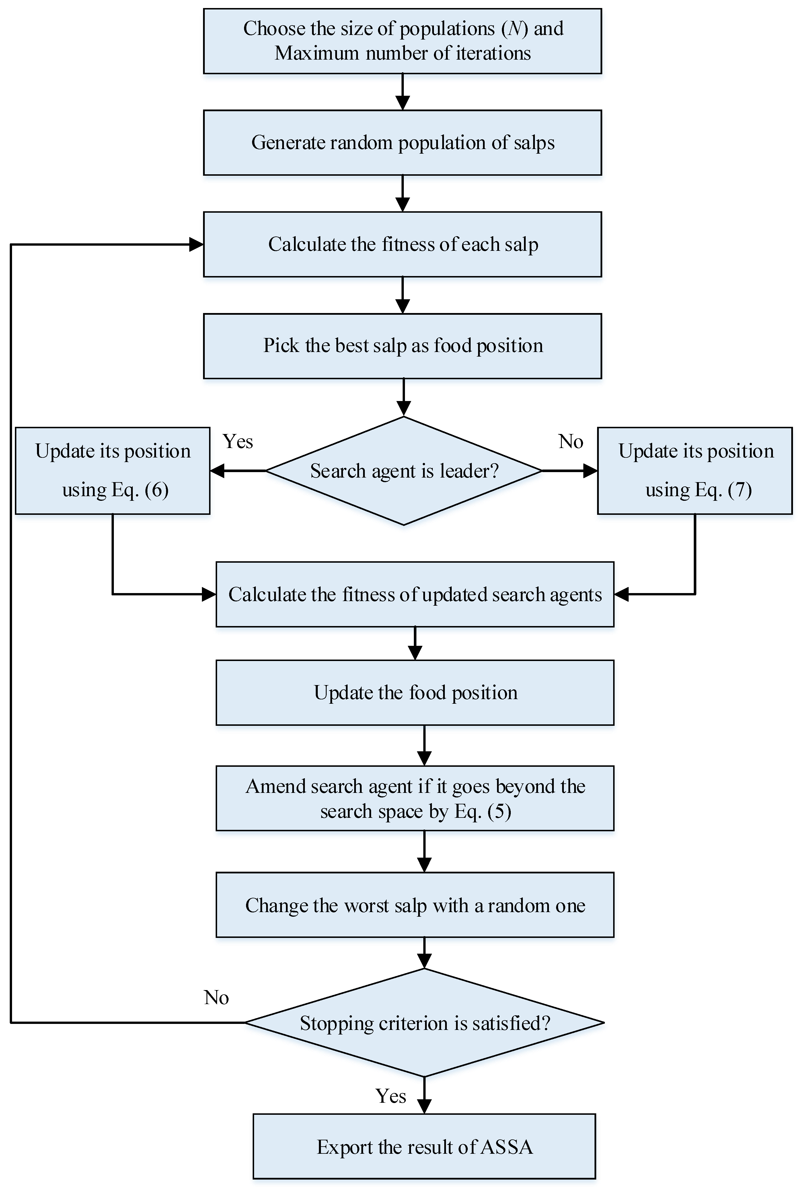
In the proposed ASSA, half of the population is considered as leaders, and the remaining salps are followers, which improves the algorithm’s performance and exploring capabilities. The following equation is then used to update the position of the leader salps:
The leaders adjust their positions in response to the state of the food source, as well as their previous position, as shown in Equation (6).
This process increases exploration while also allowing the SSA to conduct a more powerful global search across the entire search space. To improve the proposed ASSA’s search efficiency, the followers update their positions according to the following equation:
In addition, in the suggested ASSA, at each iterative process, the worst salp with the highest objective function value is replaced with a completely random salp. The flowchart of the proposed ASSA is shown in Figure 1.
4. Model Verification
A set of numerical reference test functions was used in this section to compare and confirm the achievement and effectiveness of the proposed adaptive salp swarm algorithm (ASSA). In the empirical evidence literature, these functions have commonly been used to determine the performance of optimizers [51,52].
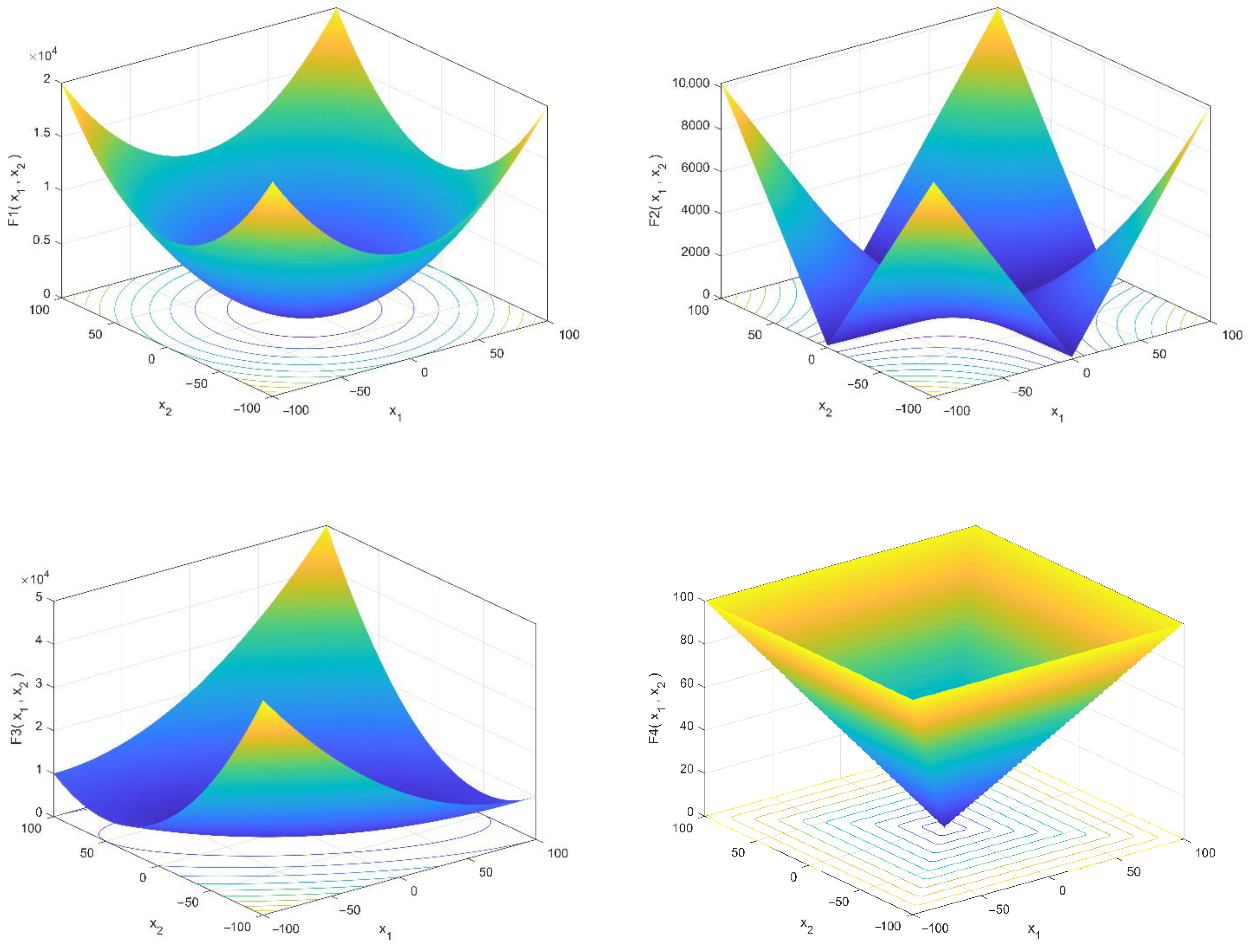
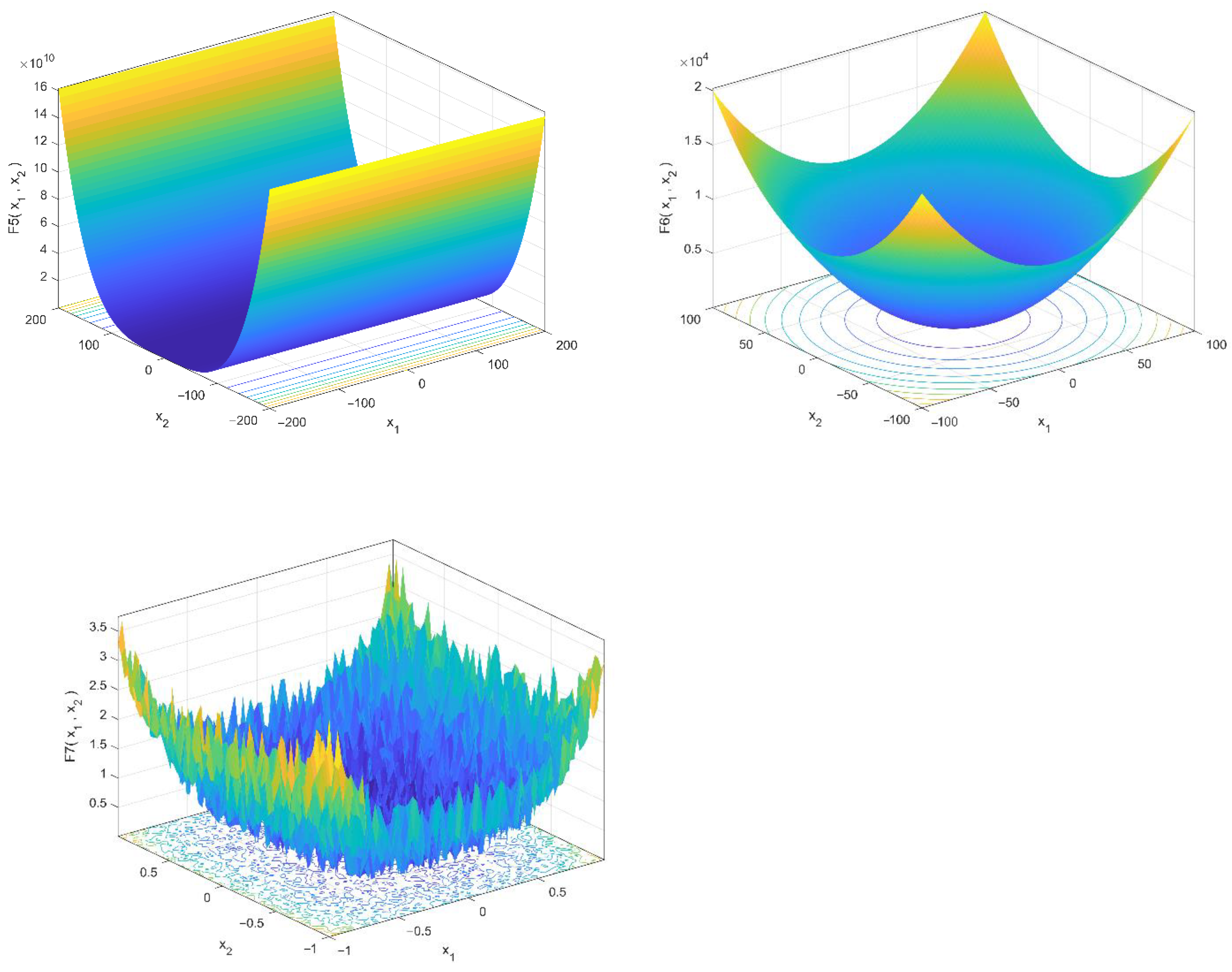
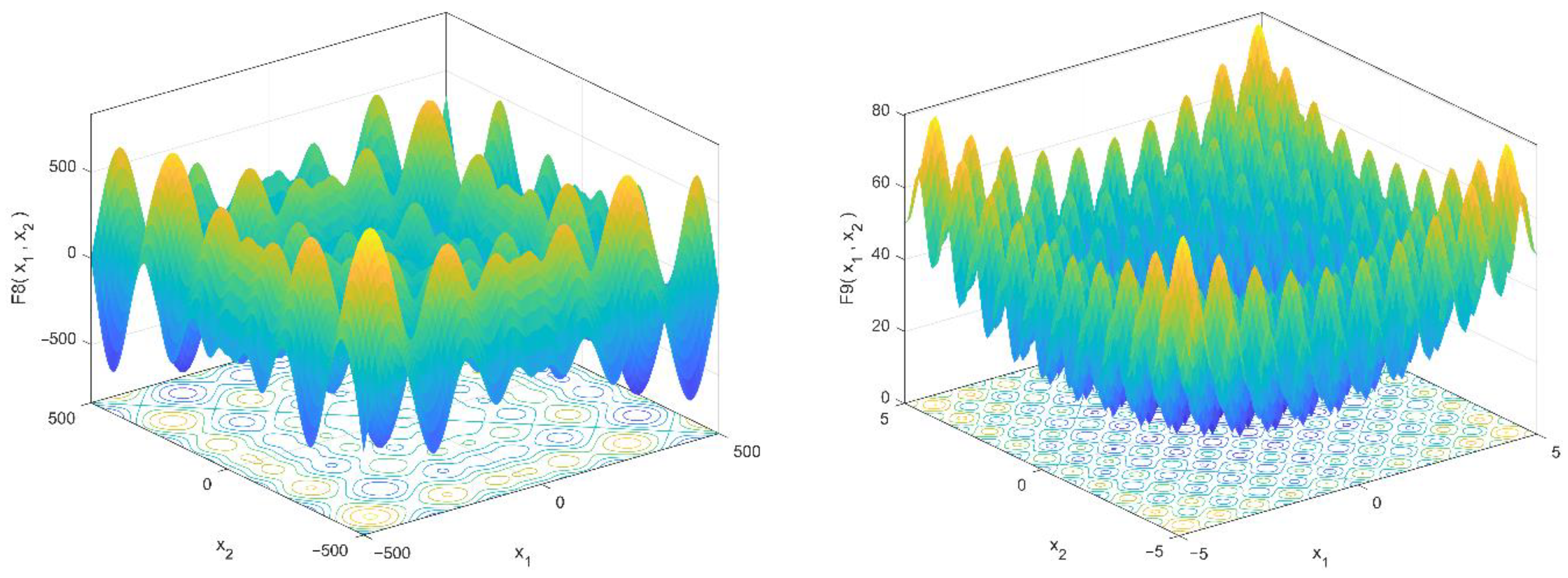
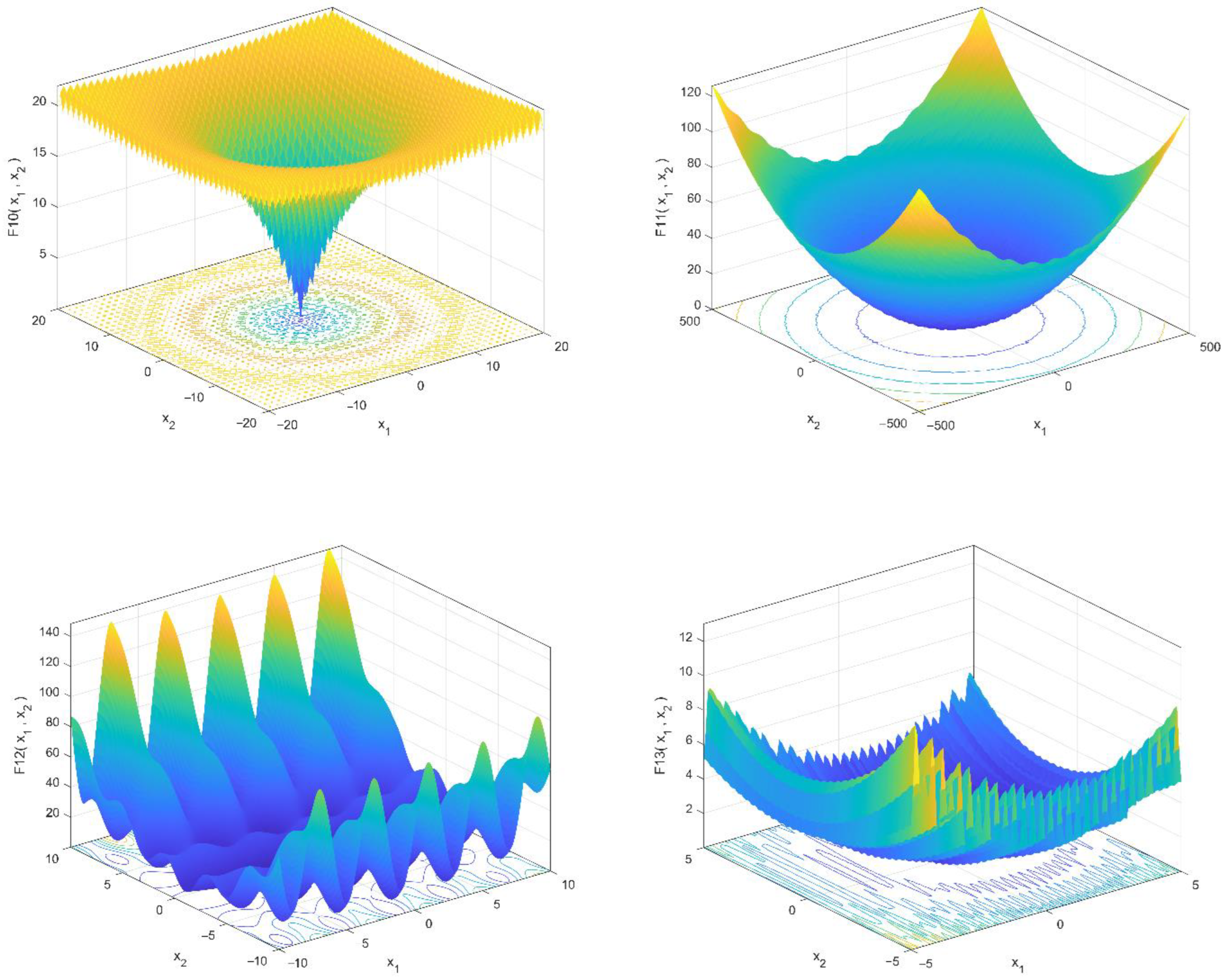
The mathematical models and characteristics of these test functions are shown in Table 2 and Table 3. This standard set was divided into two categories: (1) unimodal functions with a single global best for testing the algorithm convergence pace and enslavement ability and (2) multimodal functions with multiple local minimums and a global ideal for testing an algorithm’s local optima avoidance and exploratory capacity. MATLAB R2020b was used to create the suggested algorithms. All these functions should be minimized. Furthermore, all the functions had dimensions of 30. Three-dimensional drawings of these benchmark functions are illustrated in Figure 2 and Figure 3.
The proposed ASSA was compared to the original SSA, as well as to some well-known optimization methods, such as the genetic algorithm developed by [53], the particle swarm optimization (PSO) proposed by [54], the firefly algorithm (FA) introduced by [55], the multiverse optimizer (MVO) developed by [56], and the tunicate swarm algorithm (TSA) introduced by [52]. For all methodologies, the sizes of the solutions (N) and the maximum number of iterations (tmax) were set to 30 and 1000, respectively, in order to make fair comparisons between them.
Because the results of a single run of a metaheuristic method are stochastic, they may be incorrect. As a result, statistical analysis should be performed in order to provide a fair comparison and evaluate an algorithm’s efficacy. To address this issue, 30 runs for the mentioned methods were performed, with the results presented in Table 4 and Table 5.
Table 4 and Table 5 show that, for all the functions, the ASSA could provide better solutions in terms of mean value of the objective functions than the conventional SSA, as well as the other optimization techniques. The results also showed that the mean and standard deviation of the ASSA were significantly lower than those of the other strategies, indicating that the algorithm was stable. The ASSA outperformed both the standard method and alternative optimization approaches, according to the findings.
In order to obtain significant effectiveness between two or more algorithms, a nonparametric Wilcoxon’s rank sum test is often used [57]. In this study, a pairwise comparison was performed using the best results from 30 runs of each algorithm. The Wilcoxon’s rank sum test returned the p-value, the sum of the positive ranks (R+), and the sum of the negative ranks (R−). Table 6 shows the results of the Wilcoxon’s rank sum test for all the benchmark functions. The p-value is the smallest level of significance for detecting differences. In this study, the level of significance was set at 0.05 (α = 0.05). If the p-value was smaller than 0.05, it meant that the better result achieved by the best method in each pairwise comparison was statistically significant and was not obtained by chance. However, there was no significant difference between the two examined methods if the p-value was greater than 0.05. Such a result is indicated with “NA” in the “win” rows of Table 6. In addition, if the R+ was greater than the R−, the ASSA had a better performance than the alternative technique. Otherwise, the ASSA had a poor performance, and the other approach had a better performance [58].
According to the findings of the Wilcoxon’s rank sum test in Table 6, the pairwise comparison of the ASSA and the SSA in the optimization of thirteen test functions demonstrated that the new approach outperformed the original method in all thirteen cases. Similarly, in the other pairwise comparisons, the ASSA provided better results for the majority of the test suite. As a result of the nonparametric statistical analysis, the ASSA created much better answers and performed significantly better than the other techniques.
5. Foundation Optimization
A shallow spread foundation, as an essential geotechnical structure, must safely and reliably support the superstructure, guarantee stability against soil-bearing capacity failings and excessive settlement, and reduce concrete stresses. Aside from these design criteria, spread footings must meet a number of other criteria: they must have enough shear and moment capacities in both the long and short dimensions; the load-carrying capacity of the foundation must not be surpassed; and the reinforcing steel configuration must meet all building code criteria [59]. The foundation optimization problem requires determining the objective function, layout constraint, and design variables, which are discussed in the following subsections.
5.1. Objective Function
The total cost of the spread footing was the study’s objective function, which can be expressed mathematically as follows:
5.2. Design Variables
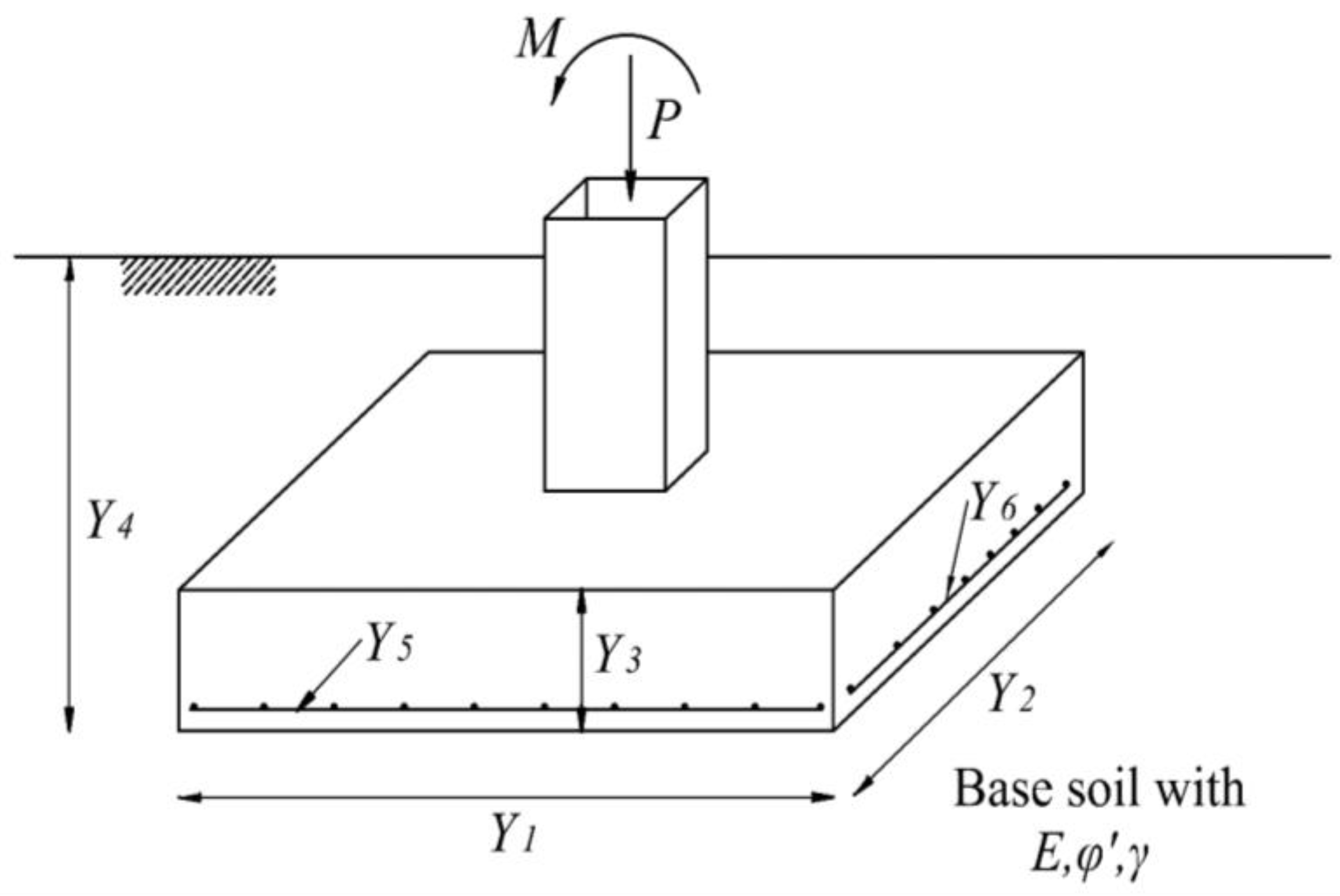
Figure 4 depicts the design features for the given model. The design variables were divided into two categories: those that described geometric dimensions and those that described steel reinforcement. As shown in Figure 4, there were four spatial design variables that reflected the foundation dimensions: the foundation’s length (Y1), the width (Y2), the thickness (Y3), and the embedment’s depth (Y4). The steel reinforcement also had two design variables: the longitudinal reinforcement (Y5) and the transverse reinforcement (Y6).
5.3. Design Constraints
While optimizing and designing a reinforced concrete footing, both structural and geotechnical limit states should be considered. Two different geotechnical limit states are the bearing capacity of the surrounding geo-material and the permitted settlement of the footing. The shear capacity of the footing (one- and two-way shear), flexural capacity, and reinforcement limitation are all structural limit states. The structural limit states are investigated using ACI 318-11 specifications [59]. Service loads are commonly used to satisfy geotechnical limit states. Even so, factored loads can be used for structural limit states. Table 8 provides a list of both structural and geotechnical limit states.
6. Retaining Structure Optimization
Reinforced concrete retaining walls are structures that are built to withstand lateral soil pressure as the land elevation changes. The retaining structure design process necessitates several considerations, such as structural dimensions, material characteristics, and needed reinforcement. Generally, the designer’s experience plays a critical role in the cost-effective and safe design of these structures. However, the optimum design of retaining walls is independent of user experience, and the results satisfy both safety and economy.
6.1. Objective Functions
In the case of retaining structure optimization, the total construction cost of the retaining wall was considered as an objective function that incorporated the cost of materials, as well as labor and installation costs, that could be represented as follows:
6.2. Design Variables
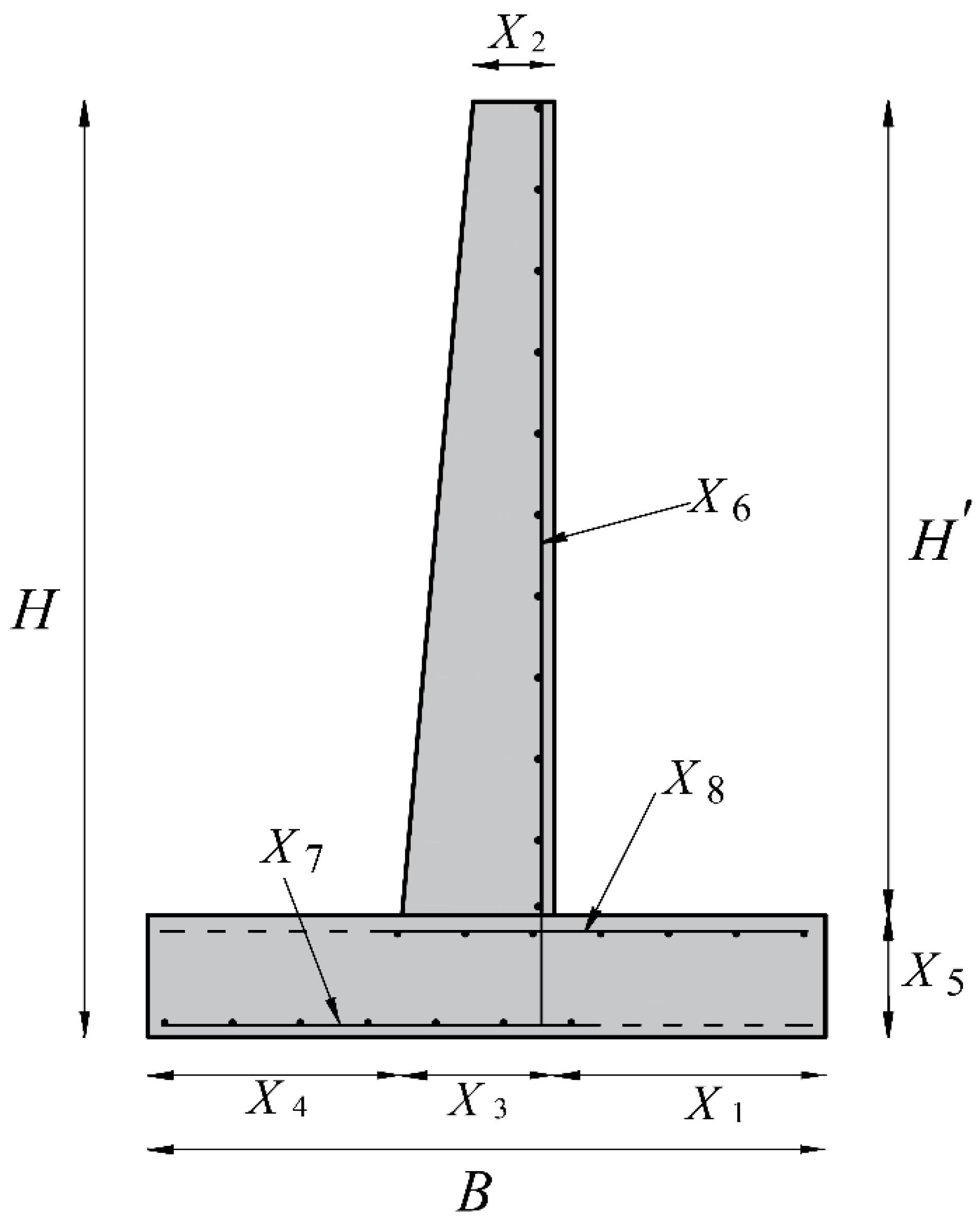
Figure 5 depicts the retaining wall model’s cross-section, design variables, and external load. As shown in this diagram, the dimensions of the retaining wall are represented by five geometric design variables: the heel width, represented by X1; the top stem thickness, represented by X2; the bottom stem thickness, represented by X3; the toe width, represented by X4; and the base slab thickness, represented by X5. Three additional design features are included in the steel reinforcement of the various sections of the retaining wall. The vertical steel reinforcement in the stem is designated as X6, the horizontal steel reinforcement in the toe is designated as X7, and the horizontal steel reinforcement in the heel is designated as X8. B is the foundation’s base width, H is the wall’s total height, and H′ is the stem’s height.
6.3. Design Constraints
7. Design Examples
This section investigates numerical problems of geotechnical structures in order to evaluate the ASSA performance. To address the current inquiry, a MATLAB code was developed to computerize the design approach based on the ACI 318-11 specifications, as stated earlier [59].
In order to consider the constraints and transform a constrained optimization to an unconstrained problem, a penalty function method was used in this paper:
where F(X) is the penalized objective function, f(X) is the problem’s original objective function presented in (8) and (9), and g(X) is the problem’s constraints presented in Table 7 and Table 10 for the spread footing and retaining wall, respectively. r is a penalty factor considered equal to 1000, l is the power of the penalty function considered equal to 2, and p is the total number of constraints.
To demonstrate the efficacy of the proposed technique, the findings were compared to state-of-the-art algorithms such as particle swarm optimization (PSO) and the firefly algorithm (FA) in the following cases. The maximum number of iterations in any algorithm was assumed to be 1000. Because of the stochastic behavior of the metaheuristics in the following experiments, all the algorithms were run 30 times, and the best results of the analyses for the minimum cost obtained by each method are reported.
7.1. Spread Footing Optimization
The first two design examples were concerned with the best design for a dry sand inner surface spread footing. Table 14 lists the other input parameters for such case studies.
The presented procedure solved the problem by combining all the previously mentioned algorithms. Table 15 and Table 16 show the best results of the analyses for the lowest cost.
Table 15 and Table 16 show that the optimization findings computed by the proposed ASSA were lower than those calculated by the conventional SSA and other approaches, indicating that the new method was effective. Table 15 shows that, contrary to popular belief that the best shape for a footing under vertical load is square, a rectangular footing provided a more cost-effective design.
7.2. Retaining Structure Optimization
The optimal design of two retaining walls with heights of 4 and 6 m was the subject of this section. Table 17 lists the other parameters that were required for this example.
Table 18 and Table 19 show that, when compared to the traditional SSA and other methods, the ASSA may be able to provide a better solution by calculating lower values of the objective functions. It can be observed that the ASSA’s best price was relatively lower than that of the SSA and significantly lower than that of the PSO and FA. However, additional experiments revealed that increasing the maximum number of iterations reduced the distinctions between the algorithm results. The fact that the best solution was found in the first iteration was due to the effective modification of the algorithm proposed in this study. The modified algorithm demonstrated a much-enhanced efficacy.
In order to determine the statistical significance of the comparative results between the considered algorithms in all the design examples, a nonparametric Wilcoxon’s rank sum test was performed between the results. In this regard, utilizing the results obtained from 30 runs of each method, a pairwise comparison was conducted. According to the results of the Wilcoxon’s rank sum test in Table 20, the pairwise comparison between the ASSA and the SSA revealed that, in the optimization of four design examples, the new method had superior performances in three cases. In addition, for design example 3, both methods were statistically equivalent. Similarly, in the other pairwise comparisons, the ASSA provided better results. Therefore, the nonparametric statistical analysis proved that the ASSA generated significantly better solutions and, comparatively, had a superior performance over the other algorithms.
8. Conclusions
The primary objective of this study was to introduce an adaptive version of the salp swarm algorithm (ASSA). Two new equations for the leader- and follower-updating positions were introduced to improve the proposed ASSA’s search and discovery abilities. In the standard SSA, the leading salp modifies its position based on a single point, which is the food location. However, due to a lack of knowledge about the real position of the food location, the algorithm may be locked at the local optimum. To overcome this weakness and to improve the exploration ability of the algorithm, in the proposed ASSA, half of the population was considered as leaders, which adjusted their positions not only based on the food location but also based on their previous positions. In addition, instead of the constant value considered in an SSA for follower-position-updating, in the ASSA, a random value was proposed. In addition, at each iteration of the optimization process, the ASSA replaced the worst salp, yielding the highest fitness value with a randomly generated salp. A statistical analysis was carried out in order to make an accurate assessment of the new algorithm’s performance. The proposed method was shown to perform admirably in terms of accuracy, stability, and robustness when tested on some well-known unimodal and multimodal test functions. The paper’s second goal was to automate a cost-effective design process for spread foundations and retaining walls. A computer program in Matlab was developed to reduce the cost of retaining structures and spread footings. On four case studies of these structures, the proposed method was compared to a classical SSA and some state-of-the-art metaheuristic algorithms. Given the final results, it was demonstrated that the ASSA outperformed the other techniques and should be able to provide better optimal results. The new method concurrently satisfied geotechnical and structural limit states while simultaneously providing a cost-effective design.
Author Contributions
M.K.: methodology, software, and data curation. A.I.: investigation and writing—original draft preparation. A.M.: conceptualization and methodology. S.K.: resources and writing—original draft preparation. M.L.N.: supervision, project administration, validation, funding acquisition, and final draft preparation. All authors have read and agreed to the published version of the manuscript.
Funding
This research received no external funding.
Institutional Review Board Statement
Not applicable.
Informed Consent Statement
Not applicable.
Data Availability Statement
The data that support the findings of this study are available from the corresponding author upon request.
Conflicts of Interest
This research work abides by the highest standards of ethics, professionalism, and collegiality. All authors have no explicit or implicit conflict of interest of any kind related to this manuscript.
References
- Cheng, Y.M.; Li, L.; Chi, S.-C.; Wei, W. Particle swarm optimization algorithm for the location of the critical non-circular failure surface in two-dimensional slope stability analysis. Comput. Geotech. 2007, 34, 92–103. [Google Scholar] [CrossRef]
- Gandomi, A.; Kashani, A.; Zeighami, F. Retaining wall optimization using interior search algorithm with different bound constraint handling. Int. J. Numer. Anal. Methods Geomech. 2017, 41, 1304–1331. [Google Scholar] [CrossRef]
- Khajehzadeh, M.; Taha, M.R.; El-Shafie, A.; Eslami, M. Search for critical failure surface in slope stability analysis by gravitational search algorithm. Int. J. Phys. Sci. 2011, 6, 5012–5021. [Google Scholar]
- Kashani, A.R.; Gandomi, M.; Camp, C.V.; Gandomi, A.H. Optimum design of shallow foundation using evolutionary algorithms. Soft Comput. 2020, 24, 6809–6833. [Google Scholar] [CrossRef]
- Almazán-Covarrubias, J.H.; Peraza-Vázquez, H.; Peña-Delgado, A.F.; García-Vite, P.M. An Improved Dingo Optimization Algorithm Applied to SHE-PWM Modulation Strategy. Appl. Sci. 2022, 12, 992. [Google Scholar] [CrossRef]
- Agresta, A.; Baioletti, M.; Biscarini, C.; Caraffini, F.; Milani, A.; Santucci, V. Using Optimisation Meta-Heuristics for the Roughness Estimation Problem in River Flow Analysis. Appl. Sci. 2021, 11, 10575. [Google Scholar] [CrossRef]
- Gandomi, A.H.; Kashani, A.R. Construction cost minimization of shallow foundation using recent swarm intelligence techniques. IEEE Trans. Ind. Inform. 2017, 14, 1099–1106. [Google Scholar] [CrossRef]
- Nigdeli, S.M.; Bekdaş, G.; Yang, X.-S. Metaheuristic optimization of reinforced concrete footings. KSCE J. Civ. Eng. 2018, 22, 4555–4563. [Google Scholar] [CrossRef] [Green Version]
- Eslami, M.; Shareef, H.; Mohamed, A.; Khajehzadeh, M. Optimal location of PSS using improved PSO with chaotic sequence. In Proceedings of the International Conference on Electrical, Control and Computer Engineering 2011 (InECCE), Kuantan, Malaysia, 21–22 June 2011; pp. 253–258. [Google Scholar]
- Delice, Y.; Aydoğan, E.K.; Özcan, U.; İlkay, M.S. A modified particle swarm optimization algorithm to mixed-model two-sided assembly line balancing. J. Intell. Manuf. 2017, 28, 23–36. [Google Scholar] [CrossRef]
- Cheng, Y.; Li, L.; Lansivaara, T.; Chi, S.; Sun, Y. An improved harmony search minimization algorithm using different slip surface generation methods for slope stability analysis. Eng. Optim. 2008, 40, 95–115. [Google Scholar] [CrossRef]
- Khajehzadeh, M.; Taha, M.R.; Eslami, M. Multi-objective optimisation of retaining walls using hybrid adaptive gravitational search algorithm. Civ. Eng. Environ. Syst. 2014, 31, 229–242. [Google Scholar] [CrossRef]
- Ji, Y.; Tu, J.; Zhou, H.; Gui, W.; Liang, G.; Chen, H.; Wang, M. An adaptive chaotic sine cosine algorithm for constrained and unconstrained optimization. Complexity 2020, 2020, 6084917. [Google Scholar] [CrossRef]
- Hegazy, A.E.; Makhlouf, M.; El-Tawel, G.S. Improved salp swarm algorithm for feature selection. J. King Saud Univ. Comput. Inf. Sci. 2020, 32, 335–344. [Google Scholar] [CrossRef]
- Gao, W. Modified ant colony optimization with improved tour construction and pheromone updating strategies for traveling salesman problem. Soft Comput. 2021, 25, 3263–3289. [Google Scholar] [CrossRef]
- Duan, D.; Poursoleiman, R. Modified teaching-learning-based optimization by orthogonal learning for optimal design of an electric vehicle charging station. Util. Policy 2021, 72, 101253. [Google Scholar] [CrossRef]
- Li, L.-L.; Liu, Z.-F.; Tseng, M.-L.; Zheng, S.-J.; Lim, M.K. Improved tunicate swarm algorithm: Solving the dynamic economic emission dispatch problems. Appl. Soft Comput. 2021, 108, 107504. [Google Scholar] [CrossRef]
- Ali, M.H.; Kamel, S.; Hassan, M.H.; Tostado-Véliz, M.; Zawbaa, H.M. An improved wild horse optimization algorithm for reliability based optimal DG planning of radial distribution networks. Energy Rep. 2022, 8, 582–604. [Google Scholar] [CrossRef]
- Goh, A. Search for critical slip circle using genetic algorithms. Civ. Eng. Environ. Syst. 2000, 17, 181–211. [Google Scholar] [CrossRef]
- Zolfaghari, A.R.; Heath, A.C.; McCombie, P.F. Simple genetic algorithm search for critical non-circular failure surface in slope stability analysis. Comput. Geotech. 2005, 32, 139–152. [Google Scholar] [CrossRef]
- Chan, C.M.; Zhang, L.; Ng, J.T. Optimization of pile groups using hybrid genetic algorithms. J. Geotech. Geoenviron. Eng. 2009, 135, 497–505. [Google Scholar] [CrossRef]
- Kahatadeniya, K.S.; Nanakorn, P.; Neaupane, K.M. Determination of the critical failure surface for slope stability analysis using ant colony optimization. Eng. Geol. 2009, 108, 133–141. [Google Scholar] [CrossRef]
- Khajehzadeh, M.; Taha, M.R.; El-Shafie, A.; Eslami, M. Modified particle swarm optimization for optimum design of spread footing and retaining wall. J. Zhejiang Univ. Sci. A 2011, 12, 415–427. [Google Scholar] [CrossRef]
- Camp, C.V.; Akin, A. Design of retaining walls using big bang–big crunch optimization. J. Struct. Eng. 2012, 138, 438–448. [Google Scholar] [CrossRef]
- Camp, C.V.; Assadollahi, A. CO2 and cost optimization of reinforced concrete footings using a hybrid big bang-big crunch algorithm. Struct. Multidiscip. Optim. 2013, 48, 411–426. [Google Scholar] [CrossRef]
- Khajehzadeh, M.; Taha, M.R.; Eslami, M. A new hybrid firefly algorithm for foundation optimization. Natl. Acad. Sci. Lett. 2013, 36, 279–288. [Google Scholar] [CrossRef]
- Kang, F.; Li, J.; Ma, Z. An artificial bee colony algorithm for locating the critical slip surface in slope stability analysis. Eng. Optim. 2013, 45, 207–223. [Google Scholar] [CrossRef]
- Kashani, A.R.; Gandomi, A.H.; Mousavi, M. Imperialistic competitive algorithm: A metaheuristic algorithm for locating the critical slip surface in 2-dimensional soil slopes. Geosci. Front. 2016, 7, 83–89. [Google Scholar] [CrossRef] [Green Version]
- Gordan, B.; Jahed Armaghani, D.; Hajihassani, M.; Monjezi, M. Prediction of seismic slope stability through combination of particle swarm optimization and neural network. Eng. Comput. 2016, 32, 85–97. [Google Scholar] [CrossRef]
- Aydogdu, I. Cost optimization of reinforced concrete cantilever retaining walls under seismic loading using a biogeography-based optimization algorithm with Levy flights. Eng. Optim. 2017, 49, 381–400. [Google Scholar] [CrossRef]
- Gandomi, A.; Kashani, A.; Mousavi, M.; Jalalvandi, M. Slope stability analysis using evolutionary optimization techniques. Int. J. Numer. Anal. Methods Geomech. 2017, 41, 251–264. [Google Scholar] [CrossRef]
- Mahdiyar, A.; Hasanipanah, M.; Armaghani, D.J.; Gordan, B.; Abdullah, A.; Arab, H.; Majid, M.Z.A. A Monte Carlo technique in safety assessment of slope under seismic condition. Eng. Comput. 2017, 33, 807–817. [Google Scholar] [CrossRef]
- Chen, H.; Asteris, P.G.; Jahed Armaghani, D.; Gordan, B.; Pham, B.T. Assessing dynamic conditions of the retaining wall: Developing two hybrid intelligent models. Appl. Sci. 2019, 9, 1042. [Google Scholar] [CrossRef] [Green Version]
- Koopialipoor, M.; Jahed Armaghani, D.; Hedayat, A.; Marto, A.; Gordan, B. Applying various hybrid intelligent systems to evaluate and predict slope stability under static and dynamic conditions. Soft Comput. 2019, 23, 5913–5929. [Google Scholar] [CrossRef]
- Yang, H.; Koopialipoor, M.; Armaghani, D.J.; Gordan, B.; Khorami, M.; Tahir, M. Intelligent design of retaining wall structures under dynamic conditions. Steel Compos. Struct. Int. J. 2019, 31, 629–640. [Google Scholar]
- Xu, C.; Gordan, B.; Koopialipoor, M.; Armaghani, D.J.; Tahir, M.; Zhang, X. Improving performance of retaining walls under dynamic conditions developing an optimized ANN based on ant colony optimization technique. IEEE Access 2019, 7, 94692–94700. [Google Scholar] [CrossRef]
- Himanshu, N.; Burman, A. Determination of critical failure surface of slopes using particle swarm optimization technique considering seepage and seismic loading. Geotech. Geol. Eng. 2019, 37, 1261–1281. [Google Scholar] [CrossRef]
- Kalemci, E.N.; İkizler, S.B.; Dede, T.; Angın, Z. Design of reinforced concrete cantilever retaining wall using Grey wolf optimization algorithm. Structures 2020, 23, 245–253. [Google Scholar] [CrossRef]
- Kaveh, A.; Hamedani, K.B.; Bakhshpoori, T. Optimal design of reinforced concrete cantilever retaining walls utilizing eleven meta-heuristic algorithms: A comparative study. Period. Polytech. Civ. Eng. 2020, 64, 156–168. [Google Scholar] [CrossRef]
- Sharma, S.; Saha, A.K.; Lohar, G. Optimization of weight and cost of cantilever retaining wall by a hybrid metaheuristic algorithm. Eng. Comput. 2021, 1–27. [Google Scholar] [CrossRef]
- Kaveh, A.; Seddighian, M.R. Optimization of Slope Critical Surfaces Considering Seepage and Seismic Effects Using Finite Element Method and Five Meta-Heuristic Algorithms. Period. Polytech. Civ. Eng. 2021, 65, 425–436. [Google Scholar] [CrossRef]
- Temur, R. Optimum design of cantilever retaining walls under seismic loads using a hybrid TLBO algorithm. Geomech. Eng. 2021, 24, 237–251. [Google Scholar]
- Li, S.; Wu, L. An improved salp swarm algorithm for locating critical slip surface of slopes. Arab. J. Geosci. 2021, 14, 359. [Google Scholar] [CrossRef]
- Khajehzadeh, M.; Keawsawasvong, S.; Sarir, P.; Khailany, D.K. Seismic Analysis of Earth Slope Using a Novel Sequential Hybrid Optimization Algorithm. Period. Polytech. Civ. Eng. 2022, 66, 355–366. [Google Scholar] [CrossRef]
- Arabali, A.; Khajehzadeh, M.; Keawsawasvong, S.; Mohammed, A.H.; Khan, B. An Adaptive Tunicate Swarm Algorithm for Optimization of Shallow Foundation. IEEE Access 2022, 10, 39204–39219. [Google Scholar] [CrossRef]
- Khajehzadeh, M.; Keawsawasvong, S.; Nehdi, M.L. Effective hybrid soft computing approach for optimum design of shallow foundations. Sustainability 2022, 14, 1847. [Google Scholar] [CrossRef]
- Khajehzadeh, M.; Kalhor, A.; Tehrani, M.S.; Jebeli, M. Optimum design of retaining structures under seismic loading using adaptive sperm swarm optimization. Struct. Eng. Mech. 2022, 81, 93–102. [Google Scholar]
- Kashani, A.R.; Camp, C.V.; Azizi, K.; Rostamian, M. Multi-objective optimization of mechanically stabilized earth retaining wall using evolutionary algorithms. Int. J. Numer. Anal. Methods Geomech. 2022, 46, 1433–1465. [Google Scholar] [CrossRef]
- Mirjalili, S.; Gandomi, A.H.; Mirjalili, S.Z.; Saremi, S.; Faris, H.; Mirjalili, S.M. Salp Swarm Algorithm: A bio-inspired optimizer for engineering design problems. Adv. Eng. Softw. 2017, 114, 163–191. [Google Scholar] [CrossRef]
- Zhao, X.; Yang, F.; Han, Y.; Cui, Y. An opposition-based chaotic salp swarm algorithm for global optimization. IEEE Access 2020, 8, 36485–36501. [Google Scholar] [CrossRef]
- Zervoudakis, K.; Tsafarakis, S. A mayfly optimization algorithm. Comput. Ind. Eng. 2020, 145, 106559. [Google Scholar] [CrossRef]
- Kaur, S.; Awasthi, L.K.; Sangal, A.; Dhiman, G. Tunicate swarm algorithm: A new bio-inspired based metaheuristic paradigm for global optimization. Eng. Appl. Artif. Intell. 2020, 90, 103541. [Google Scholar] [CrossRef]
- Holland, J.H. Genetic algorithms. Sci. Am. 1992, 267, 66–73. [Google Scholar] [CrossRef]
- Kennedy, J.; Eberhart, R. Particle swarm optimization. In Proceedings of the ICNN’95-International Conference on Neural Networks, Perth, Australia, 27 November–1 December 1995; pp. 1942–1948. [Google Scholar]
- Yang, X.S. Firefly algorithms for multimodal optimization. Lect. Notes Comput. Sci. 2009, 5792, 169–178. [Google Scholar]
- Mirjalili, S.; Mirjalili, S.M.; Hatamlou, A. Multi-verse optimizer: A nature-inspired algorithm for global optimization. Neural Comput. Appl. 2016, 27, 495–513. [Google Scholar] [CrossRef]
- Derrac, J.; García, S.; Molina, D.; Herrera, F. A practical tutorial on the use of nonparametric statistical tests as a methodology for comparing evolutionary and swarm intelligence algorithms. Swarm Evol. Comput. 2011, 1, 3–18. [Google Scholar] [CrossRef]
- Toz, M. Chaos-based Vortex Search algorithm for solving inverse kinematics problem of serial robot manipulators with offset wrist. Appl. Soft Comput. 2020, 89, 106074. [Google Scholar] [CrossRef]
- ACI Committee 318. ACI 318-11 Building Code Requirements for Structural Concrete; American Concrete Institute: Farmington Hills, MI, USA, 2011. [Google Scholar]
- Wang, Y.; Kulhawy, F.H. Economic design optimization of foundations. J. Geotech. Geoenviron. Eng. 2008, 134, 1097–1105. [Google Scholar] [CrossRef]
- Yepes, V.; Gonzalez-Vidosa, F.; Alcala, J.; Villalba, P. CO2-optimization design of reinforced concrete retaining walls based on a VNS-threshold acceptance strategy. J. Comput. Civ. Eng. 2012, 26, 378–386. [Google Scholar] [CrossRef] [Green Version]
- Bowles, J. Foundation Analysis and Design; McGraw-Hill: New York, NY, USA, 1982. [Google Scholar]
Figure 1.
Flowchart of ASSA.

Figure 2.
3-D versions of unimodal benchmark functions.


Figure 3.
3-D versions of multimodal benchmark functions.


Figure 4.
Design variables of the footing.

Figure 5.
Design variables of the retaining structure.

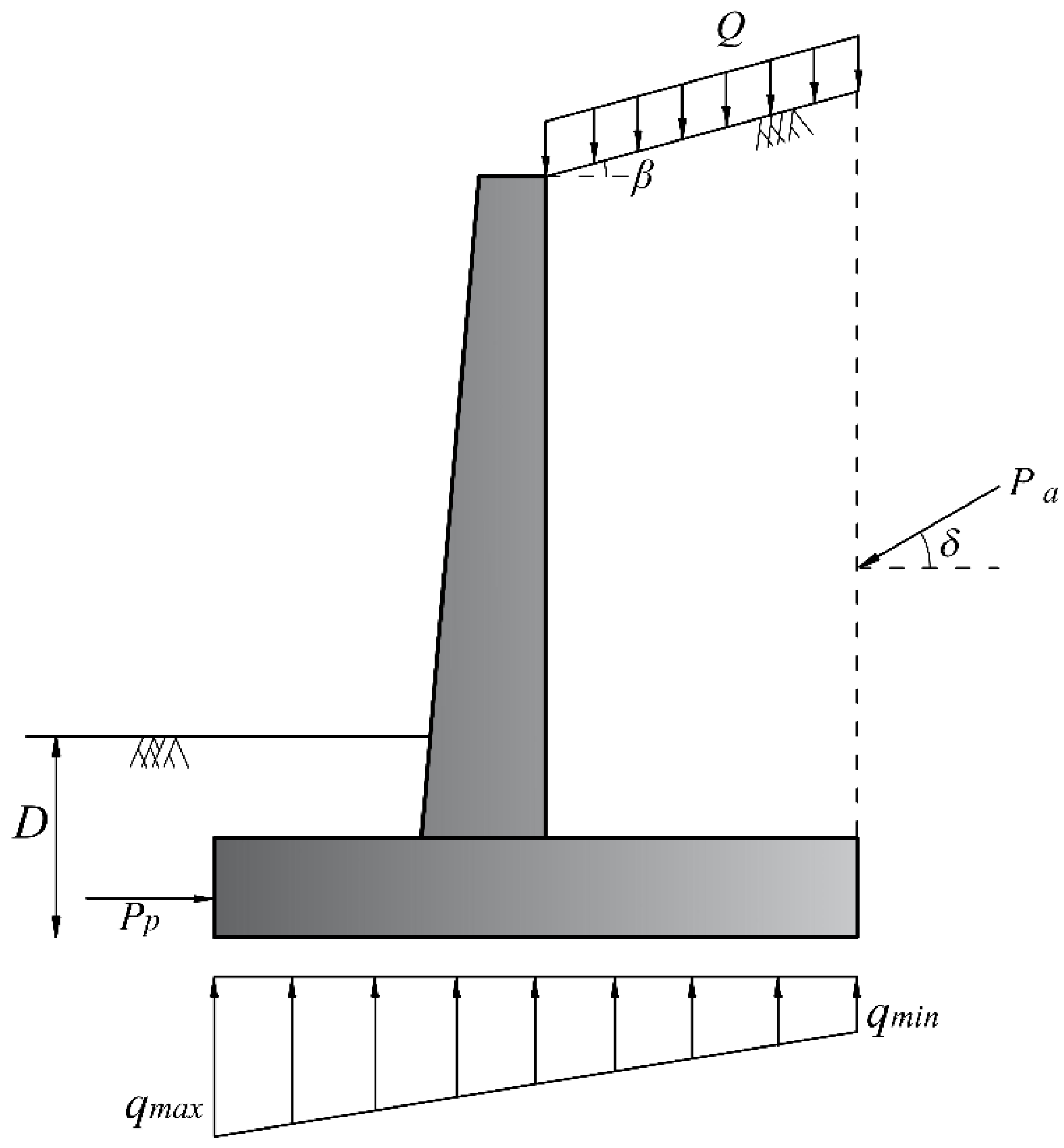
Figure 6.
Forces acting on the retaining wall.


Table 1.
Application of metaheuristic algorithms for geotechnical engineering problems.
| Author, Year | Reference | Optimization Method | Application |
|---|---|---|---|
| Goh, 2000 | [19] | Genetic algorithm | Locate the critical circular slip surface in slope stability analysis |
| Zolfaghari, Heath, and McCombie, 2005 | [20] | Genetic algorithm | Search for critical noncircular failure surface in slope stability analysis |
| Cheng et al., 2007 | [1] | Particle swarm optimization | Analyze two-dimensional slope stability |
| Cheng et al., 2008 | [11] | Improved harmony search algorithm | Analyze slope stability |
| Chan, Zhang, and Ng, 2009 | [21] | Hybrid genetic algorithms | Optimize pile groups |
| Kahatadeniya, Nanakorn, and Neaupane, 2009 | [22] | Ant colony optimization | Determine the critical failure surface of earth slope |
| Khajehzadeh et al., 2011 | [23] | Modified particle swarm optimization | Optimize design of spread footing and retaining wall |
| Camp and Akin, 2012 | [24] | Big bang–big crunch optimization | Optimize design of retaining wall |
| Camp and Assadollahi, 2013 | [25] | Hybrid big bang–big crunch algorithm | Optimize CO2 and cost of reinforced concrete footings |
| Khajehzadeh et al., 2013 | [26] | Hybrid firefly algorithm | Multi-objective optimization of foundations |
| Kang, Li, and Ma, 2013 | [27] | Artificial bee colony algorithm | Locate the critical slip surface in slope stability analysis |
| Khajehzadeh, Taha, and Eslami, 2014 | [12] | Hybrid adaptive gravitational search algorithm | Multi-objective optimization of retaining walls |
| Kashani, Gandomi, and Mousavi, 2016 | [28] | Imperialistic competitive algorithm | Locate the critical slip surface of earth slope |
| Gordan et al., 2016 | [29] | Particle swarm optimization and neural network | Predict seismic slope stability |
| Gandomi and Kashani, 2017 | [7] | Accelerated particle swarm optimization, firefly algorithm, Levy-flight krill herd, whale optimization algorithm, ant lion optimizer, grey wolf optimizer, moth–flame optimization algorithm, and teaching–learning-based optimization algorithm | Minimize construction cost of shallow foundation |
| Aydogdu, 2017 | [30] | Biogeography-based optimization algorithm | Optimize cost of retaining wall |
| Gandomi et al., 2017 | [31] | Genetic algorithm, differential evolution, evolutionary strategy, and biogeography-based optimization | Analyze slope stability |
| Mahdiyar et al., 2017 | [32] | Monte Carlo simulation technique | Assess safety of slope |
| Gandomi, Kashani, and Zeighami, 2017 | [2] | Interior search algorithm | Optimize retaining wall |
| Chen et al., 2019 | [33] | Hybrid imperialist competitive algorithm and artificial neural network | Predict safety factor values of retaining walls |
| Koopialipoor et al., 2019 | [34] | Imperialist competitive algorithm, genetic algorithm, particle swarm optimization, and artificial bee colony combined with artificial neural network | Predict slope stability under static and dynamic conditions |
| Yang et al., 2019 | [35] | Neural network system | Design retaining wall structures based on smart and optimal systems |
| Xu et al., 2019 | [36] | Hybrid artificial neural network and ant colony optimization | Assess dynamic conditions of retaining wall structures |
| Himanshu and Burman, 2019 | [37] | Particle swarm optimization | Determine critical failure surface considering seepage and seismic loading |
| Kalemci et al., 2020 | [38] | Grey wolf optimization algorithm | Optimize retaining walls |
| Kaveh, Hamedani, and Bakhshpoori, 2020 | [39] | Eleven metaheuristic algorithms | Optimize design of cantilever retaining walls |
| Kashani et al., 2020 | [4] | Differential algorithm, evolution strategy, and biogeography-based optimization algorithm | Optimize design of shallow foundation |
| Sharma, Saha, and Lohar, 2021 | [40] | Hybrid butterfly and symbiosis organism search algorithm | Optimize retaining wall |
| Kaveh and Seddighian, 2021 | [41] | Black hole mechanics optimization, firefly algorithm, evolution strategy, and sine cosine algorithm | Optimize slope critical surfaces considering seepage and seismic effects |
| Temur, 2021 | [42] | Teaching–learning-based optimization | Optimize retaining wall |
| Li and Wu, 2021 | [43] | Improved salp swarm algorithm | Locate critical slip surface of slopes |
| Khajehzadeh, Keawsawasvong, et al., 2022 | [44] | Hybrid tunicate swarm algorithm and pattern search | Seismic analysis of earth slope |
| Arabali et al., 2022 | [45] | Adaptive tunicate swarm algorithm | Optimize construction cost and CO2 emissions of shallow foundation |
| Khajehzadeh, Keawsawasvong, and Nehdi, 2022 | [46] | Artificial neural network combined with rat swarm optimization | Predict the ultimate bearing capacity of shallow foundations and their optimum design |
| Khajehzadeh, Kalhor, et al., 2022 | [47] | Adaptive sperm swarm optimization | Optimize design of retaining structures under seismic load |
| Kashani et al., 2022 | [48] | Multi-objective particle swarm optimization, multi-objective multiverse optimization and Pareto envelope-based selection algorithm | Multi-objective optimization of mechanically stabilized earth retaining wall |
Table 2.
Description of unimodal benchmark functions.
| Function | Range | n (Dim) | |
|---|---|---|---|
| 0 | 30 | ||
| 0 | 30 | ||
| 0 | 30 | ||
| 0 | 30 | ||
| 0 | 30 | ||
| 0 | 30 | ||
| 0 | 30 |
Table 3.
Description of multimodal benchmark functions.
| Function | Range | n (Dim) | |
|---|---|---|---|
| 428.9829 × n | 30 | ||
| 0 | 30 | ||
| 0 | 30 | ||
| 0 | 30 | ||
| 0 | 30 | ||
| 0 | 30 |
Table 4.
Comparison of different methods in solving unimodal test functions.
| F | Index | ASSA | SSA | GA | PSO | FA | MVO | TSA |
|---|---|---|---|---|---|---|---|---|
| F1 | Mean | 2.23 × 10−227 | 3.29 × 10⁻⁷ | 1.95 × 10⁻¹² | 4.98 × 10⁻⁹ | 7.11 × 10⁻³ | 2.81 × 10⁻¹ | 8.31 × 10−56 |
| Std. | 0.00 | 5.92 × 10⁻⁷ | 2.01 × 10⁻¹¹ | 1.40 × 10⁻⁸ | 3.21 × 10⁻³ | 1.11 × 10⁻¹ | 1.02 × 10−58 | |
| F2 | Mean | 5.96 × 10−105 | 1.911 | 6.53 × 10⁻¹⁸ | 7.29 × 10⁻⁴ | 4.34 × 10⁻¹ | 3.96 × 10⁻¹ | 8.36 × 10⁻³⁵ |
| Std. | 1.91 × 10−104 | 1.614 | 5.10 × 10⁻¹⁷ | 1.84 × 10⁻³ | 1.84 × 10⁻¹ | 1.41 × 10⁻¹ | 9.86 × 10⁻³⁵ | |
| F3 | Mean | 3.27 × 10−180 | 1.50 × 10³ | 7.70 × 10⁻¹⁰ | 14.0 | 1.66 × 10³ | 43.1 | 1.51 × 10⁻¹⁴ |
| Std. | 0.00 | 7.07 × 10² | 7.36 × 10⁻⁹ | 7.13 | 6.72 × 10² | 8.97 | 6.55 × 10⁻¹⁴ | |
| F4 | Mean | 1.56 × 10−104 | 2.44 × 10⁻⁵ | 91.7 | 6.00 × 10⁻¹ | 1.11 × 10⁻¹ | 8.80 × 10⁻¹ | 1.95 × 10⁻⁵ |
| Std. | 3.47 × 10−105 | 1.89 × 10⁻⁵ | 56.7 | 1.72 × 10⁻¹ | 4.75 × 10⁻² | 2.50 × 10⁻¹ | 4.49 × 10⁻⁴ | |
| F5 | Mean | 2.56 × 10⁻¹ | 1.36 × 10² | 5.57 × 10² | 49.3 | 79.7 | 1.18 × 10² | 28.4 |
| Std. | 4.78 × 10⁻¹ | 1.54 × 10² | 41.6 | 38.9 | 73.9 | 1.43 × 10² | 8.40 × 10⁻¹ | |
| F6 | Mean | 3.76 × 10⁻⁷ | 5.72 × 10⁻⁷ | 3.15 × 10⁻¹ | 6.92 × 10⁻² | 6.94 × 10⁻³ | 2.02 × 10⁻² | 3.67 |
| Std. | 1.23 × 10⁻⁷ | 2.44 × 10⁻⁷ | 9.98 × 10⁻² | 2.87 × 10⁻² | 3.61 × 10⁻³ | 7.43 × 10⁻³ | 3.35 × 10⁻¹ | |
| F7 | Mean | 2.71 × 10⁻⁶ | 8.82 × 10⁻⁵ | 6.79 × 10⁻⁴ | 8.94 × 10⁻² | 6.62 × 10⁻² | 5.24 × 10⁻² | 1.80 × 10⁻³ |
| Std. | 2.33 × 10⁻⁶ | 6.94 × 10⁻⁵ | 3.29 × 10⁻³ | 2.06 × 10⁻² | 4.23 × 10⁻² | 1.37 × 10⁻² | 4.62 × 10⁻⁴ |
Table 5.
Comparison of different methods in solving multimodal test functions.
| F | Index | ASSA | SSA | GA | PSO | FA | MVO | TSA |
|---|---|---|---|---|---|---|---|---|
| F8 | Mean | –1.21 × 10⁴ | –7.46 × 10³ | –5.11 × 10³ | –6.01 × 10³ | –5.85 × 10³ | –6.92 × 10³ | –7.89 × 10³ |
| Std. | 4.89 × 10² | 6.34 × 10² | 4.37 × 10² | 1.30 × 10³ | 1.61 × 10³ | 9.19 × 10² | 599.2 | |
| F9 | Mean | 0.00 | 55.45 | 1.23 × 10⁻¹ | 47.2 | 15.1 | 1.01× 10² | 151.4 |
| Std. | 0.00 | 18.27 | 41.1 | 10.3 | 12.5 | 18.9 | 35.87 | |
| F10 | Mean | 8.88 × 10⁻¹⁶ | 2.84 | 5.31 × 10⁻¹¹ | 3.86 × 10⁻² | 4.58 × 10⁻² | 1.15 | 2.409 |
| Std. | 0.00 | 6.58 × 10⁻¹ | 1.11 × 10⁻¹⁰ | 2.11 × 10⁻¹ | 1.20 × 10⁻² | 7.87 × 10⁻¹ | 1.392 | |
| F11 | Mean | 0.00 | 2.29 × 10⁻¹ | 3.31 × 10⁻⁶ | 5.50 × 10⁻³ | 4.23 × 10⁻³ | 5.74 × 10⁻¹ | 7.7 × 10⁻³ |
| Std. | 0.00 | 1.29 × 10⁻¹ | 4.23 × 10⁻⁵ | 7.39 × 10⁻³ | 1.29 × 10⁻³ | 1.12 × 10⁻¹ | 5.7 × 10⁻³ | |
| F12 | Mean | 2.31 × 10⁻⁵ | 6.82 | 9.16 × 10⁻⁸ | 1.05 × 10⁻² | 3.13 × 10⁻⁴ | 1.27 | 6.373 |
| Std. | 2.46 × 10⁻⁵ | 2.72 | 4.88 × 10⁻⁷ | 2.06 × 10⁻² | 1.76 × 10⁻⁴ | 1.02 | 3.458 | |
| F13 | Mean | 1.44 × 10⁻⁴ | 21.31 | 6.39 × 10⁻² | 4.03 × 10⁻¹ | 2.08 × 10⁻³ | 6.60 × 10⁻² | 2.897 |
| Std. | 1.95 × 10⁻⁴ | 16.99 | 4.49 × 10⁻² | 5.39 × 10⁻¹ | 9.62 × 10⁻⁴ | 4.33 × 10⁻² | 6.43 × 10⁻¹ |
Table 6.
Results of Wilcoxon’s rank sum test for benchmark functions.
| Fun. | Index | ASSA vs. SSA | ASSA vs. GA | ASSA vs. PSO | ASSA vs. FA | ASSA vs. MVO | ASSA vs. TSA |
|---|---|---|---|---|---|---|---|
| F1 | p-val. | 2.0 × 10⁻⁶ | 2.0 × 10⁻⁶ | 2.0 × 10⁻⁶ | 2.0 × 10⁻⁶ | 2.0 × 10⁻⁶ | 2.0 × 10⁻⁶ |
| R+ | 465 | 465 | 465 | 465 | 465 | 465 | |
| R− | 0.0 | 0.0 | 0.0 | 0.0 | 0.0 | 0.0 | |
| Win | ASSA | ASSA | ASSA | ASSA | ASSA | ASSA | |
| F2 | p-val. | 2.0 × 10⁻⁶ | 2.0 × 10⁻⁶ | 2.0 × 10⁻⁶ | 2.0 × 10⁻⁶ | 2.0 × 10⁻⁶ | 2.0 × 10⁻⁶ |
| R+ | 465 | 465 | 465 | 465 | 465 | 465 | |
| R− | 0.0 | 0.0 | 0.0 | 0.0 | 0.0 | 0.0 | |
| Win | ASSA | ASSA | ASSA | ASSA | ASSA | ASSA | |
| F3 | p-val. | 2.0 × 10⁻⁶ | 2.0 × 10⁻⁶ | 2.0 × 10⁻⁶ | 2.0 × 10⁻⁶ | 2.0 × 10⁻⁶ | 2.0 × 10⁻⁶ |
| R+ | 465 | 465 | 465 | 465 | 465 | 465 | |
| R− | 0.0 | 0.0 | 0.0 | 0.0 | 0.0 | 0.0 | |
| Win | ASSA | ASSA | ASSA | ASSA | ASSA | ASSA | |
| F4 | p-val. | 2.0 × 10⁻⁶ | 2.0 × 10⁻⁶ | 2.0 × 10⁻⁶ | 2.0 × 10⁻⁶ | 2.0 × 10⁻⁶ | 2.0 × 10⁻⁶ |
| R+ | 465 | 465 | 465 | 465 | 465 | 465 | |
| R− | 0.0 | 0.0 | 0.0 | 0.0 | 0.0 | 0.0 | |
| Win | ASSA | ASSA | ASSA | ASSA | ASSA | ASSA | |
| F5 | p-val. | 2.0 × 10⁻⁶ | 2.0 × 10⁻⁶ | 2.0 × 10⁻⁶ | 2.0 × 10⁻⁶ | 2.0 × 10⁻⁶ | 2.0 × 10⁻⁶ |
| R+ | 465 | 465 | 465 | 465 | 465 | 465 | |
| R− | 0.0 | 0.0 | 0.0 | 0.0 | 0.0 | 0.0 | |
| Win | ASSA | ASSA | ASSA | ASSA | ASSA | ASSA | |
| F6 | p-val. | 6.0 × 10⁻⁶ | 2.0 × 10⁻⁶ | 2.0 × 10⁻⁶ | 2.0 × 10⁻⁶ | 2.0 × 10⁻⁶ | 2.0 × 10⁻⁶ |
| R+ | 453 | 465 | 465 | 465 | 465 | 465 | |
| R− | 12 | 0.0 | 0.0 | 0.0 | 0.0 | 0.0 | |
| Win | ASSA | ASSA | ASSA | ASSA | ASSA | ASSA | |
| F7 | p-val. | 6.0 × 10⁻⁶ | 2.0 × 10⁻⁶ | 2.0 × 10⁻⁶ | 2.0 × 10⁻⁶ | 2.0 × 10⁻⁶ | 2.0 × 10⁻⁶ |
| R+ | 453 | 465 | 465 | 465 | 465 | 465 | |
| R− | 12 | 0.0 | 0.0 | 0.0 | 0.0 | 0.0 | |
| Win | ASSA | ASSA | ASSA | ASSA | ASSA | ASSA | |
| F8 | p-val. | 2.0 × 10⁻⁶ | 2.0 × 10⁻⁶ | 2.0 × 10⁻⁶ | 2.0 × 10⁻⁶ | 2.0 × 10⁻⁶ | 2.0 × 10⁻⁶ |
| R+ | 465 | 465 | 465 | 465 | 465 | 465 | |
| R− | 0.0 | 0.0 | 0.0 | 0.0 | 0.0 | 0.0 | |
| Win | ASSA | ASSA | ASSA | ASSA | ASSA | ASSA | |
| F9 | p-val. | 2.0 × 10⁻⁶ | 2.0 × 10⁻⁶ | 2.0 × 10⁻⁶ | 2.0 × 10⁻⁶ | 2.0 × 10⁻⁶ | 2.0 × 10⁻⁶ |
| R+ | 465 | 465 | 465 | 465 | 465 | 465 | |
| R− | 0.0 | 0.0 | 0.0 | 0.0 | 0.0 | 0.0 | |
| Win | ASSA | ASSA | ASSA | ASSA | ASSA | ASSA | |
| F10 | p-val. | 2.0 × 10⁻⁶ | 2.0 × 10⁻⁶ | 2.0 × 10⁻⁶ | 2.0 × 10⁻⁶ | 2.0 × 10⁻⁶ | 2.0 × 10⁻⁶ |
| R+ | 465 | 465 | 465 | 465 | 465 | 465 | |
| R− | 0.0 | 0.0 | 0.0 | 0.0 | 0.0 | 0.0 | |
| Win | ASSA | ASSA | ASSA | ASSA | ASSA | ASSA | |
| F11 | p-val. | 2.0 × 10⁻⁶ | 2.0 × 10⁻⁶ | 2.0 × 10⁻⁶ | 2.0 × 10⁻⁶ | 2.0 × 10⁻⁶ | 2.0 × 10⁻⁶ |
| R+ | 465 | 465 | 465 | 465 | 465 | 465 | |
| R− | 0.0 | 0.0 | 0.0 | 0.0 | 0.0 | 0.0 | |
| Win | ASSA | ASSA | ASSA | ASSA | ASSA | ASSA | |
| F12 | p-val. | 2.0 × 10⁻⁶ | 2.0 × 10⁻⁶ | 2.0 × 10⁻⁶ | 2.0 × 10⁻⁶ | 2.0 × 10⁻⁶ | 2.0 × 10⁻⁶ |
| R+ | 465 | 0.0 | 465 | 465 | 465 | 465 | |
| R− | 0.0 | 465 | 0.0 | 0.0 | 0.0 | 0.0 | |
| Win | ASSA | GA | ASSA | ASSA | ASSA | ASSA | |
| F13 | p-val. | 2.0 × 10⁻⁶ | 2.0 × 10⁻⁶ | 2.0 × 10⁻⁶ | 2.0 × 10⁻⁶ | 2.0 × 10⁻⁶ | 2.0 × 10⁻⁶ |
| R+ | 465 | 465 | 465 | 465 | 465 | 465 | |
| R− | 0.0 | 0.0 | 0.0 | 0.0 | 0.0 | 0.0 | |
| Win | ASSA | ASSA | ASSA | ASSA | ASSA | ASSA | |
| Superior /Inferior/NA | 13/0/0 | 12/1/0 | 13/0/0 | 13/0/0 | 13/0/0 | 13/0/0 |
Table 7.
Spread footing assembly unit cost [60].
Table 7.
Spread footing assembly unit cost [60].
| Item | Symbol | Unit | Unit Cost (USD) |
|---|---|---|---|
| Excavation | Ce | m3 | 25.16 |
| Formwork | Cf | m2 | 51.97 |
| Reinforcement | Cs | kg | 2.16 |
| Concrete | Cc | m3 | 173.96 |
| Backfill | Cb | m3 | 3.97 |
Table 8.
Design constraints of spread footing.
| Failure Mode | Constraint |
|---|---|
| Bearing capacity | |
| Settlement of foundation | |
| Eccentricity | e ≤ Y1/6 |
| One-way (wide beam) shear | |
| Two-way (punching) shear | |
| Bending moment | |
| Minimum and maximum reinforcements | |
| Limitation of depth of embedment | 0.5 ≤ Y4 ≤ 2 |
Table 9.
Definition of parameters of Table 7.
Table 9.
Definition of parameters of Table 7.
| Parameter | Definition |
|---|---|
| qult | ultimate bearing capacity of the foundation soil |
| qmax | maximum contact pressure at the interface between the bottom of a foundation and the underlying soil |
| δall | allowable settlement of foundation |
| δ | immediate settlement of foundation |
| ϕV | shear strength reduction factor equal to 0.75 |
| f′c | compression strength of concrete |
| b0 | perimeter of critical section taken at d/2 from face of column |
| b | width of the section |
| βc | ratio of long side to short side of column section |
| αs | is equal to 40 for interior columns |
| Mu | bending moment |
| ϕM | flexure strength reduction factor equal to 0.9 |
| As | cross-sectional area of steel reinforcement |
| fy | yield strength of steel |
| ρmin | minimum reinforcement ratio |
| ρmax | maximum reinforcement ratio |
Table 10.
Basic prices considered in the analysis.
| Item | Unit | Unit Cost (USD/m) |
|---|---|---|
| Excavation | m3 | 11.41 |
| Foundation formwork | m2 | 36.82 |
| Stem formwork | m2 | 37.08 |
| Reinforcement | kg | 1.51 |
| Concrete in foundations | m3 | 104.51 |
| Concrete in stem | m3 | 118.05 |
| Backfill | m3 | 38.10 |
Table 11.
Failure modes of retaining wall.
| Failure Mode | Constraints |
|---|---|
| Sliding stability | FSS ≤ (ΣFR/ΣFd) |
| Overturning stability | FSO ≤ (ΣMR/ΣMO) |
| Bearing capacity | FSb ≤ (qult/qmax) |
| Eccentricity failure | e ≤ (B/6) |
| Toe shear | Vut ≤ Vnt |
| Toe moment | Mut ≤ Mnt |
| Heel shear | Vuh ≤ Vnh |
| Heel moment | Muh ≤ Mnh |
| Shear at bottom of stem | Vus ≤ Vns |
| Moment at bottom of stem | Mus ≤ Mns |
| Deflection at top of stem | (1/150) × H′ ≤ δmax |
| Parameter | Definition |
|---|---|
| β | backfill slop angle |
| D | depth of soil in front of the wall |
| Q | distributed surcharge load |
| Pa | active earth pressure |
| Pp | passive earth pressure |
| FSS | required factor of safety against sliding |
| FSO | required factor of safety against overturning |
| FSb | required factor of safety against bearing capacity |
| ∑FR | sum of the horizontal resisting forces |
| ∑Fd | sum of the horizontal driving forces |
| ∑MR | sum of the moments of forces that tends to resist overturning about the toe |
| ∑MO | sum of the moments of forces that tends to overturn the structure about the toe |
| ∑V | sum of the vertical forces due to the weight of wall |
| Vut | ultimate shearing force of toe |
| Vuh | ultimate shearing force of heel |
| Vus | ultimate shearing force of stem |
| Vn | nominal shear strength of concrete |
| Mut | ultimate bending moment of toe |
| Muh | ultimate bending moment of heel |
| Mus | ultimate bending moment of toe stem |
| Mn | nominal flexural strength of concrete |
| δmax | maximum deflection at the top of the stem |
Table 13.
Upper bound and lower bound for design variables of retaining wall.
| Description | Lower Bound | Upper Bound |
|---|---|---|
| Width of footing | Bmin= 0.4 H | Bmax = 0.7 H |
| Thickness of base slab | X5min= H/12 | X5max= H/10 |
| Width of toe | X4min= 0.4 H/3 | X4max= 0.7 H/3 |
| Stem thickness at top | X2min= 20 cm | - |
| Steel reinforcement ratio |
Table 14.
Input parameters for design examples 1 and 2.
| Parameter | Unit | Value for Example 1 | Value for Example 2 |
|---|---|---|---|
| Effective friction angle of base soil | degree | 35 | 30 |
| Unit weight of base soil | kN/m3 | 18.5 | 18.5 |
| Young’s modulus | MPa | 50 | 35 |
| Poisson’s ratio | − | 0.3 | 0.3 |
| Vertical dead load (D) | kN | 2000 | 4200 |
| Vertical live load (L) | kN | 1000 | 2100 |
| Moment (M) | kN-m | 0.0 | 850 |
| Concrete cover | cm | 7.0 | 7.0 |
| Yield strength of reinforcing steel | MPa | 400 | 400 |
| Compressive strength of concrete | MPa | 30 | 28 |
| Factor of safety for bearing capacity | − | 3.0 | 3.0 |
| Allowable settlement of footing | m | 0.04 | 0.04 |
Table 15.
Optimization results for design example 1.
| Design Variable | Unit | Optimum Values ASSA | Optimum Values SSA | Optimum Values FA | Optimum Values PSO |
|---|---|---|---|---|---|
| (Y1) | cm | 169.5 | 158.3 | 155.3 | 169.4 |
| (Y2) | cm | 218.8 | 248.5 | 253.1 | 219.2 |
| (Y3) | cm | 57.5 | 58.1 | 58.2 | 60 |
| (Y4) | cm | 200 | 158.2 | 200 | 200 |
| (Y5) | cm2 | 39.58 | 48.2 | 49.65 | 37.75 |
| (Y6) | cm2 | 25.13 | 21.74 | 20.94 | 23.91 |
| Objective function | USD | 1091 | 1098 | 1162 | 1108 |
Table 16.
Optimization result for design example 2.
| Design Variable | Unit | Optimum Values ASSA | Optimum Values SSA | Optimum Values FA | Optimum Values PSO |
|---|---|---|---|---|---|
| (Y1) | cm | 153 | 153.1 | 159.3 | 153.2 |
| (Y2) | cm | 833.4 | 833.2 | 819.1 | 837.6 |
| (Y3) | cm | 80.6 | 80.6 | 82.4 | 80.8 |
| (Y4) | cm | 200 | 200 | 200 | 200 |
| (Y5) | cm2 | 277.1 | 277.2 | 256.8 | 278.1 |
| (Y6) | cm2 | 20.54 | 21.1 | 24.7 | 20.6 |
| Objective function | USD | 4512 | 4520 | 4650 | 4544 |
Table 17.
Input parameters for design examples 3 and 4.
| Parameter | Unit | Value for Example 3 | Value for Example 4 |
|---|---|---|---|
| Height of stem | m | 4.0 | 6 |
| Internal friction angle of retained soil | degree | 36 | 36 |
| Internal friction angle of base soil | degree | 0.0 | 34 |
| Unit weight of retained soil | kN/m3 | 17.5 | 17.5 |
| Unit weight of base soil | kN/m3 | 18.5 | 18.5 |
| Unit weight of concrete | kN/m3 | 23.5 | 24 |
| Cohesion of base soil | kPa | 125 | 100 |
| Depth of soil in front of wall | m | 0.5 | 0.75 |
| Surcharge load | kPa | 20 | 30 |
| Backfill slop | degree | 10 | 15 |
| Concrete cover | cm | 7.0 | 7.0 |
| Yield strength of reinforcing steel | MPa | 400 | 400 |
| Compressive strength of concrete | MPa | 21 | 28 |
| Shrinkage and temporary reinforcement percent | - | 0.002 | 0.002 |
| Factor of safety for overturning stability | - | 1.5 | 1.5 |
| Factor of safety against sliding | - | 1.5 | 1.5 |
| Factor of safety for bearing capacity | - | 3.0 | 3.0 |
Table 18.
Optimization results for design example 3.
| Design Variable | Unit | Optimum Values ASSA | Optimum Values SSA | Optimum Values FA | Optimum Values PSO |
|---|---|---|---|---|---|
| (X1) | m | 0.7233 | 0.6947 | 0.6948 | 0.6436 |
| (X2) | m | 0.2 | 0.2 | 0.2 | 0.25 |
| (X3) | m | 0.4674 | 0.5 | 0.5 | 0.55 |
| (X4) | m | 0.7778 | 0.7778 | 0.7778 | 0.7778 |
| (X5) | m | 0.2727 | 0.2727 | 0.2723 | 0.2727 |
| (X6) | cm2/m | 6.67 | 6.66 | 6.66 | 6.66 |
| (X7) | cm2/m | 6.75 | 6.75 | 6.75 | 6.75 |
| (X8) | cm2/m | 6.75 | 6.75 | 6.75 | 6.75 |
| Objective function | USD/m | 822.73 | 827.02 | 860.42 | 848.17 |
Table 19.
Optimization results for design example 4.
| Design Variable | Unit | Optimum Values ASSA | Optimum Values SSA | Optimum Values FA | Optimum Values PSO |
|---|---|---|---|---|---|
| (X1) | m | 1.423 | 1.391 | 1.459 | 1.444 |
| (X2) | m | 0.25 | 0.25 | 0.246 | 0.249 |
| (X3) | m | 0.531 | 0.532 | 0.466 | 0.517 |
| (X4) | m | 0.755 | 0.772 | 0.773 | 0.774 |
| (X5) | m | 0.331 | 0.374 | 0.352 | 0.339 |
| (X6) | cm2/m | 25.38 | 25.64 | 32.21 | 27.52 |
| (X7) | cm2/m | 6.78 | 6.75 | 6.75 | 7.02 |
| (X8) | cm2/m | 7.94 | 7.47 | 7.57 | 8.39 |
| Objective function | USD/m | 1631.2 | 1643.1 | 1668.4 | 1653.9 |
Table 20.
Results of Wilcoxon’s rank sum test for design examples.
| Example No. | Index | ASSA vs. SSA | ASSA vs. FA | ASSA vs. PSO |
|---|---|---|---|---|
| Ex. 1 | p-val. | 6.0 × 10⁻⁶ | 1.73 × 10⁻⁶ | 1.73 × 10⁻⁶ |
| R+ | 453 | 465 | 465 | |
| R− | 12 | 0.0 | 0.0 | |
| Win | ASSA | ASSA | ASSA | |
| Ex. 2 | p-val. | 0.012 | 1.73 × 10⁻⁶ | 1.73 × 10⁻⁶ |
| R+ | 354 | 465 | 465 | |
| R− | 111 | 0.0 | 0.0 | |
| Win | ASSA | ASSA | ASSA | |
| Ex. 3 | p-val. | 0.106 | 1.73 × 10⁻⁶ | 1.73 × 10⁻⁶ |
| R+ | 311 | 465 | 465 | |
| R− | 154 | 0.0 | 0.0 | |
| Win | NA | ASSA | ASSA | |
| Ex. 4 | p-val. | 1.73 × 10⁻⁶ | 1.73 × 10⁻⁶ | 1.73 × 10⁻⁶ |
| R+ | 465 | 465 | 465 | |
| R− | 0.0 | 0.0 | 0.0 | |
| Win | ASSA | ASSA | ASSA | |
| Superior /Inferior/NA | 3/0/1 | 4/0/0 | 4/0/0 |
Publisher’s Note: MDPI stays neutral with regard to jurisdictional claims in published maps and institutional affiliations. |
© 2022 by the authors. Licensee MDPI, Basel, Switzerland. This article is an open access article distributed under the terms and conditions of the Creative Commons Attribution (CC BY) license (https://creativecommons.org/licenses/by/4.0/).
Share and Cite
MDPI and ACS Style
Khajehzadeh, M.; Iraji, A.; Majdi, A.; Keawsawasvong, S.; Nehdi, M.L. Adaptive Salp Swarm Algorithm for Optimization of Geotechnical Structures. Appl. Sci. 2022, 12, 6749. https://doi.org/10.3390/app12136749
AMA Style
Khajehzadeh M, Iraji A, Majdi A, Keawsawasvong S, Nehdi ML. Adaptive Salp Swarm Algorithm for Optimization of Geotechnical Structures. Applied Sciences. 2022; 12(13):6749. https://doi.org/10.3390/app12136749
Chicago/Turabian StyleKhajehzadeh, Mohammad, Amin Iraji, Ali Majdi, Suraparb Keawsawasvong, and Moncef L. Nehdi. 2022. "Adaptive Salp Swarm Algorithm for Optimization of Geotechnical Structures" Applied Sciences 12, no. 13: 6749. https://doi.org/10.3390/app12136749
Note that from the first issue of 2016, this journal uses article numbers instead of page numbers. See further details here.