
Density Prediction in Powder Bed Fusion Additive Manufacturing: Machine Learning-Based Techniques

 , , , and
Abstract
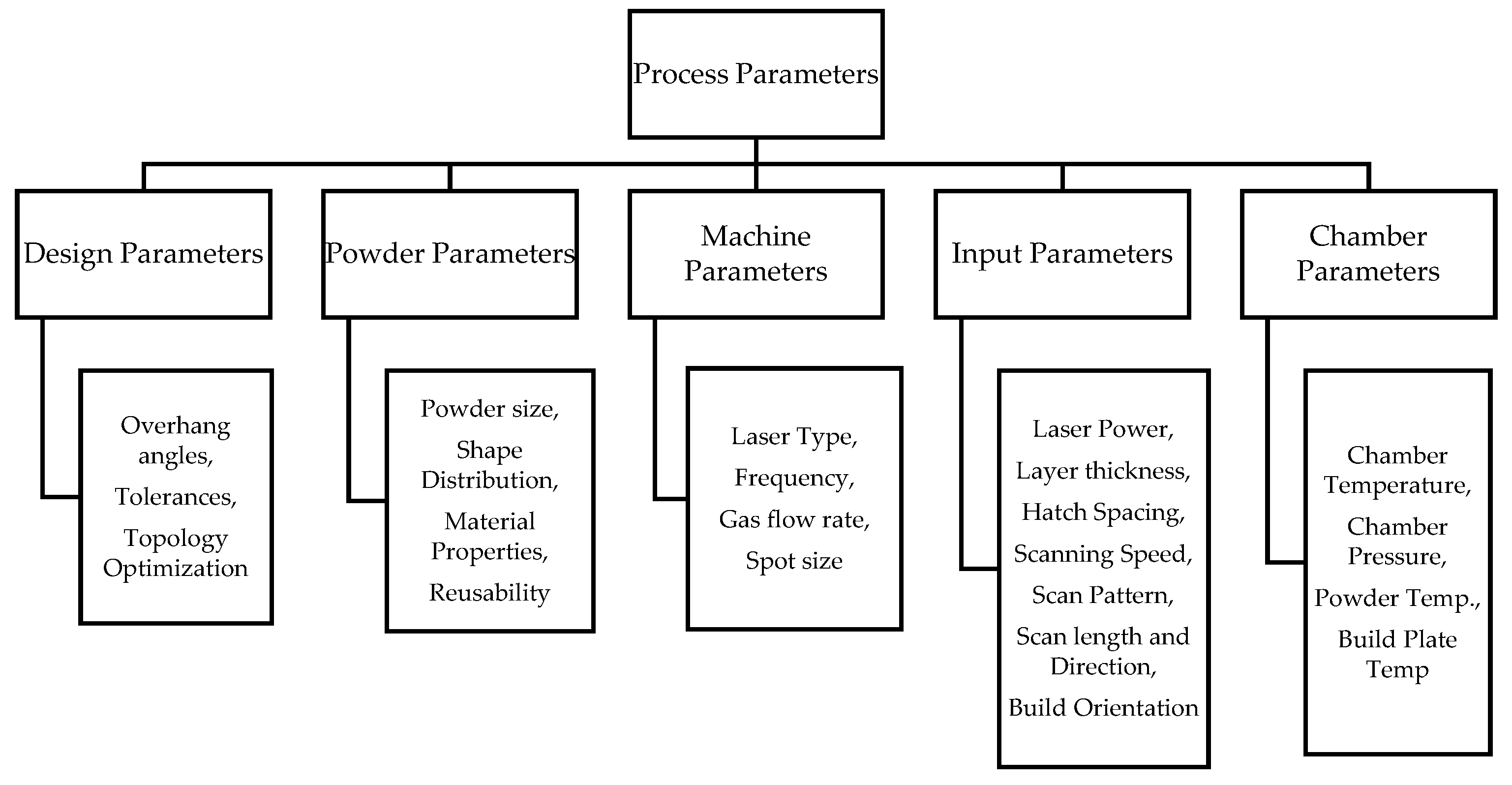
:1. Introduction
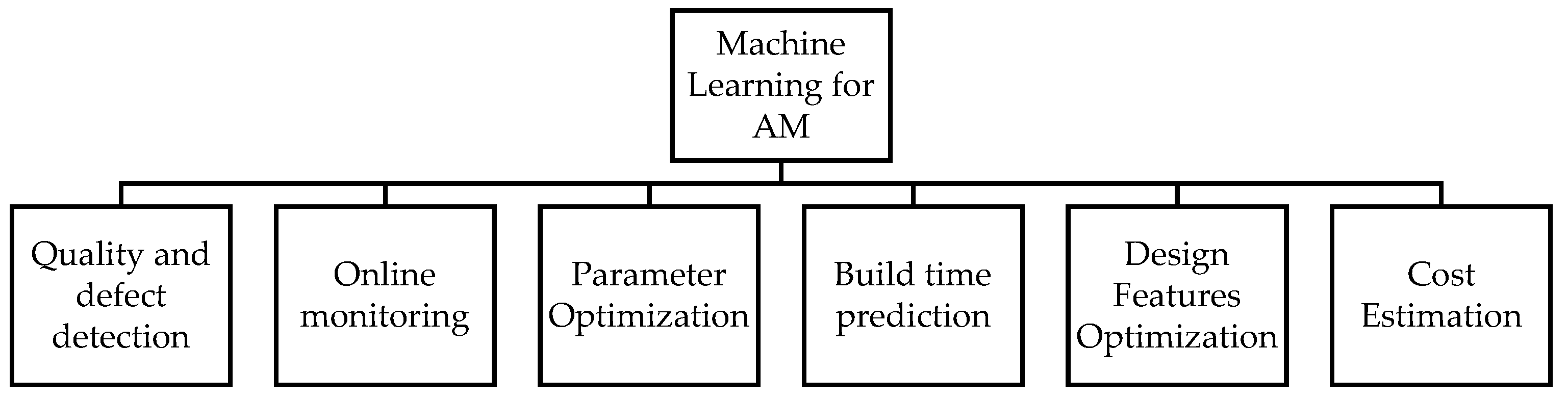
2. Literature Review
3. Methodology
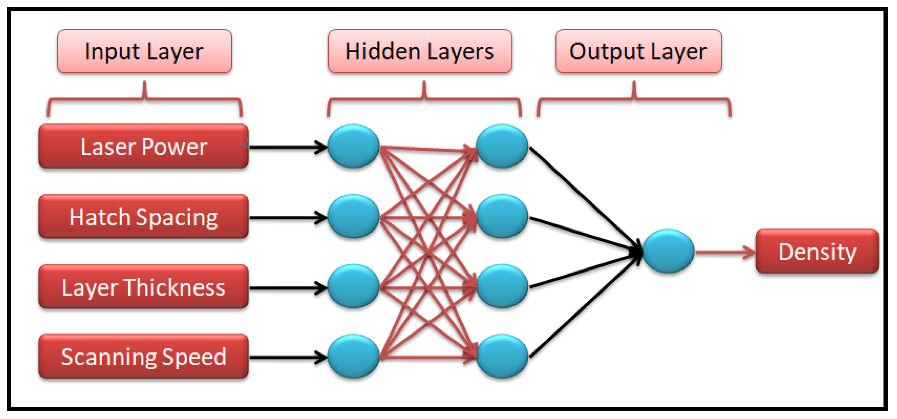
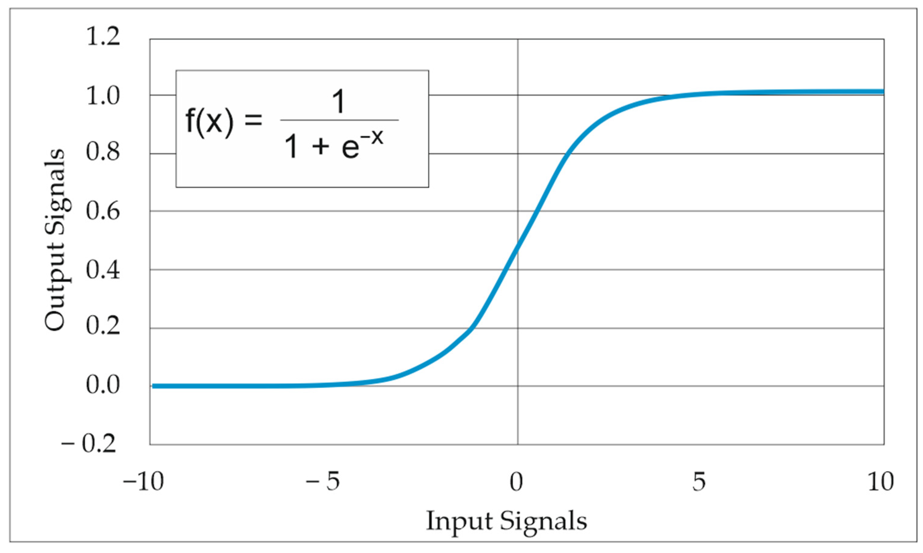
3.1. ANN
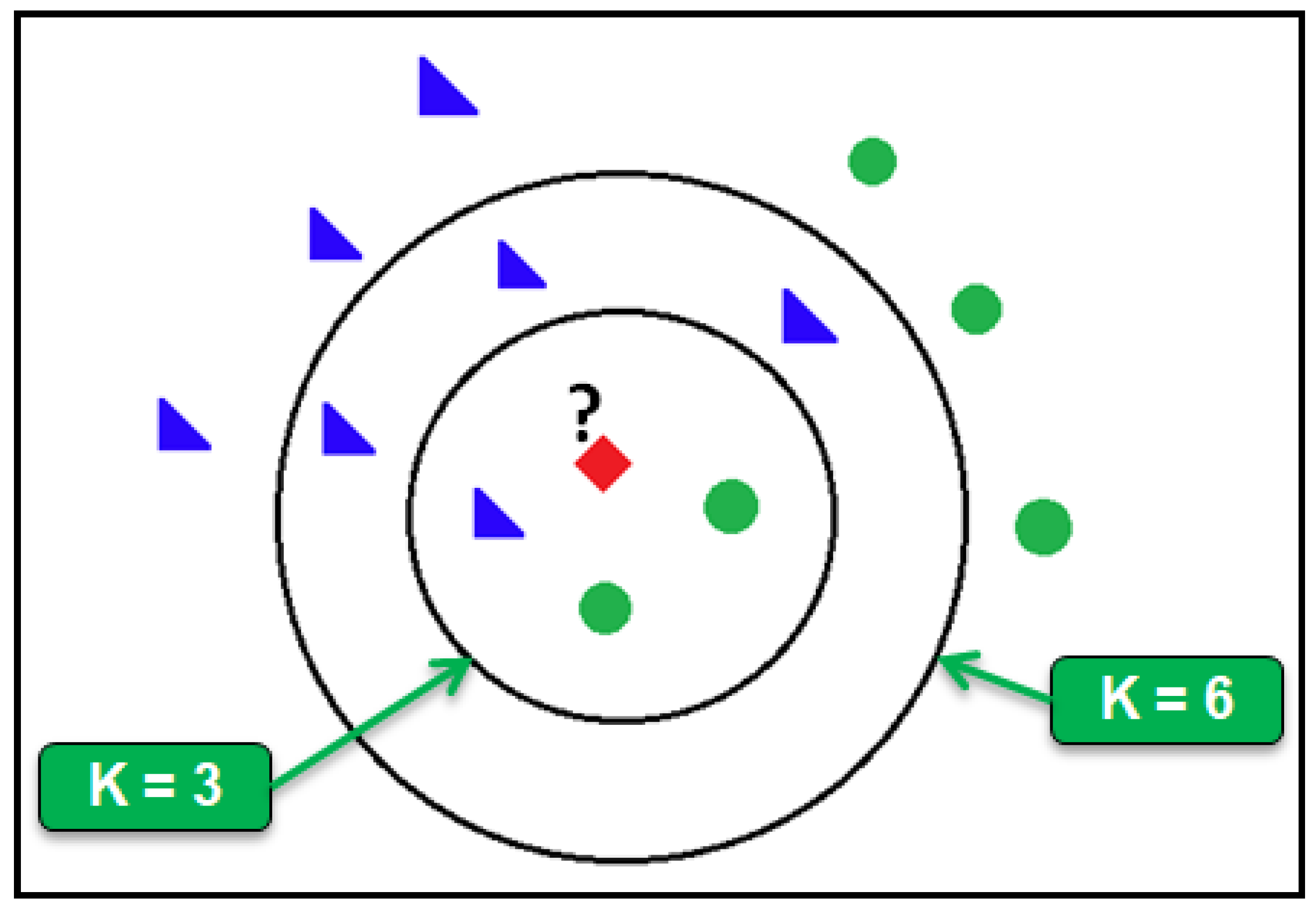
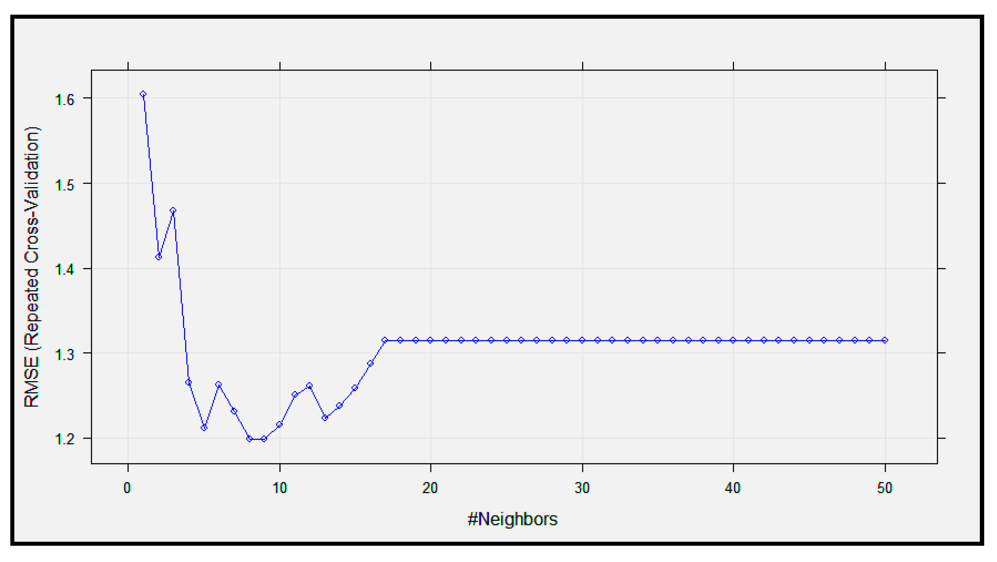
3.2. K-Nearest Neighbor
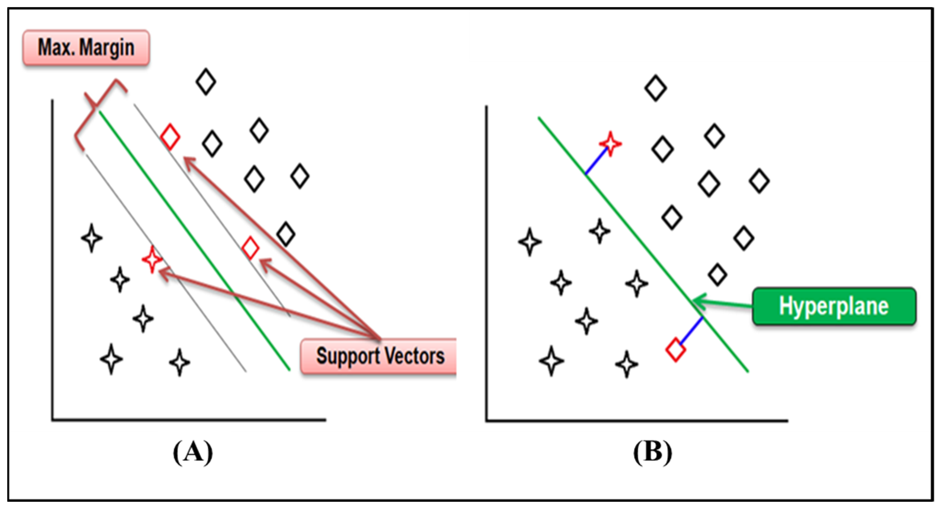
3.3. Support Vector Machine
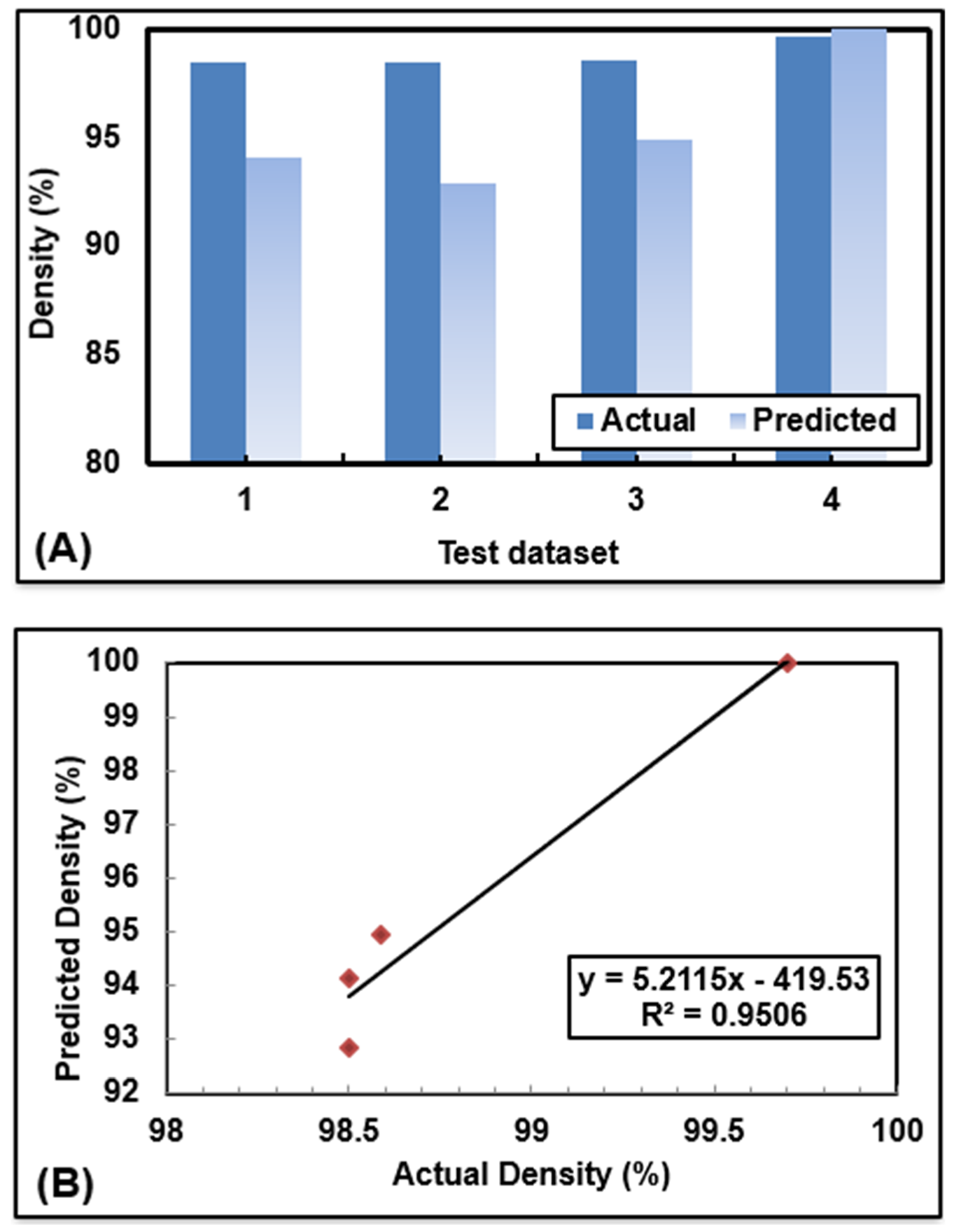
4. Results
5. Discussion
6. Conclusions
Author Contributions
Funding
Institutional Review Board Statement
Informed Consent Statement
Conflicts of Interest
Appendix A

| Inputs | Outputs | |||
|---|---|---|---|---|
| Laser Power (W) | Scanning Speed (mm/s) | Hatch Spacing (μm) | Layer Thickness (μm) | Density (%) |
| 70 | 287 | 100 | 40 | 94.6 |
| 90 | 1500 | 56 | 25 | 95 |
| 90 | 600 | 84 | 25 | 99.1 |
| 90 | 300 | 84 | 25 | 99.25 |
| 90 | 300 | 84 | 25 | 99 |
| 95 | 350 | 140 | 30 | 98 |
| 100 | 90 | 100 | 60 | 96 |
| 100 | 180 | 100 | 60 | 65 |
| 105 | 800 | 0.975 | 30 | 98.44 |
| 120 | 492 | 100 | 40 | 99.63 |
| 150 | 1250 | 80 | 30 | 96.57 |
| 150 | 714 | 140 | 30 | 97.46 |
| 150 | 750 | 120 | 30 | 98.72 |
| 150 | 1133 | 80 | 30 | 98.59 |
| 150 | 781 | 80 | 30 | 99.86 |
| 150 | 446 | 140 | 30 | 99.84 |
| 175 | 750 | 120 | 30 | 99.73 |
| 190 | 1300 | 97.5 | 30 | 99.29 |
| 190 | 800 | 97.5 | 50 | 99.12 |
| 195 | 1100 | 100 | 40 | 99.75 |
| 195 | 900 | 100 | 40 | 99.58 |
| 195 | 800 | 100 | 40 | 100 |
| 195 | 600 | 100 | 40 | 99.83 |
| 195 | 2166 | 90 | 20 | 93.24 |
| 195 | 1083 | 180 | 20 | 92.87 |
| 195 | 541 | 90 | 20 | 98 |
| 195 | 1083 | 45 | 20 | 97.36 |
| 200 | 1667 | 80 | 30 | 97.38 |
| 200 | 952 | 140 | 30 | 97.35 |
| 200 | 1198 | 140 | 30 | 99.24 |
| 200 | 1042 | 80 | 30 | 99.7 |
| 200 | 565 | 140 | 30 | 99.27 |
| 250 | 1200 | 110 | 50 | 75.24 |
| 300 | 700 | 80 | 30 | 98.5 |
| 300 | 800 | 80 | 30 | 98.5 |
| 300 | 1000 | 80 | 30 | 98.5 |
| 300 | 1200 | 80 | 30 | 94.5 |
| 350 | 650 | 110 | 50 | 99.6 |
References
- Vaezi, M.; Chianrabutra, S.; Mellor, B.; Yang, S. Multiple material additive manufacturing—Part 1: A review. Virtual Phys. Prototyp. 2013, 8, 19–50. [Google Scholar] [CrossRef]
- Jyothish Kumar, L.; Pandey, P.M.; Wimpenny, D.I. 3D Printing and Additive Manufacturing Technologies; Springer: Singapore, 2018. [Google Scholar] [CrossRef]
- Tapia, G.; Elwany, A.H.; Sang, H. Prediction of porosity in metal-based additive manufacturing using spatial Gaussian process models. Addit. Manuf. 2016, 12, 282–290. [Google Scholar] [CrossRef]
- Roy, M.; Wodo, O. Data-driven modeling of thermal history in additive manufacturing. Addit. Manuf. 2020, 32, 101017. [Google Scholar] [CrossRef]
- Zhang, M.; Sun, C.-N.; Zhang, X.; Goh, P.C.; Wei, J.; Hardacre, D.; Li, H. High cycle fatigue life prediction of laser additive manufactured stainless steel: A machine learning approach. Int. J. Fatigue 2019, 128, 105194. [Google Scholar] [CrossRef]
- Razvi, S.S.; Feng, S.; Narayanan, A.; Lee, Y.T.T.; Witherell, P. A review of machine learning applications in additive manufacturing. In Proceedings of the ASME Design Engineering Technical Conference, Anaheim, CA, USA, 18–21 August 2019. [Google Scholar]
- Meng, L.; McWilliams, B.; Jarosinski, W.; Park, H.-Y.; Jung, Y.-G.; Lee, J.; Zhang, J. Machine Learning in Additive Manufacturing: A Review. JOM 2020, 72, 2363–2377. [Google Scholar] [CrossRef]
- Wang, C.; Tan, X.P.; Tor, S.B.; Lim, C.S. Machine learning in additive manufacturing: State-of-the-art and perspectives. Addit. Manuf. 2020, 36, 101538. [Google Scholar] [CrossRef]
- Gong, X.; Zeng, D.; Groeneveld-Meijer, W.; Manogharan, G. Additive manufacturing: A machine learning model of process-structure-property linkages for machining behavior of Ti-6Al-4V. Mater. Sci. Addit. Manuf. 2022, 1, 6. [Google Scholar] [CrossRef]
- Smoqi, Z.; Gaikwad, A.; Bevans, B.; Kobir, M.H.; Craig, J.; Abul-Haj, A.; Peralta, A.; Rao, P. Monitoring and prediction of porosity in laser powder bed fusion using physics-informed meltpool signatures and machine learning. J. Mater. Process. Technol. 2022, 304, 117550. [Google Scholar] [CrossRef]
- Snow, Z.; Diehl, B.; Reutzel, E.W.; Nassar, A. Toward in-situ flaw detection in laser powder bed fusion additive manufacturing through layerwise imagery and machine learning. J. Manuf. Syst. 2021, 59, 12–26. [Google Scholar] [CrossRef]
- Liu, R.; Liu, S.; Zhang, X. A physics-informed machine learning model for porosity analysis in laser powder bed fusion additive manufacturing. Int. J. Adv. Manuf. Technol. 2021, 113, 1943–1958. [Google Scholar] [CrossRef]
- Rathi, N.K.; Rathi, N. An application of ANN for modeling and optimisation of process parameters of manufacturing process: A review. Int. J. Eng. Appl. Sci. Technol. 2020, 4, 127–134. [Google Scholar] [CrossRef]
- Stangierski, J.; Weiss, D.; Kaczmarek, A. Multiple regression models and Artificial Neural Network (ANN) as prediction tools of changes in overall quality during the storage of spreadable processed Gouda cheese. Eur. Food Res. Technol. 2019, 245, 2539–2547. [Google Scholar] [CrossRef] [Green Version]
- Abu Alfeilat, H.A.; Hassanat, A.B.A.; Lasassmeh, O.T.; Altarawneh, A.S.A.; Alhasanat, M.B.; Salman, H.S.E.; Prasath, S. Effects of Distance Measure Choice on K-Nearest Neighbor Classifier Performance: A Review. Big Data 2019, 7, 221–248. [Google Scholar] [CrossRef] [Green Version]
- Wu, D.; Wei, Y.; Terpenny, J. Predictive modelling of surface roughness in fused deposition modelling using data fusion. Int. J. Prod. Res. 2018, 57, 3992–4006. [Google Scholar] [CrossRef]
- AlFaify, A.; Hughes, J.; Ridgway, K. Controlling the porosity of 316L stainless steel parts manufactured via the powder bed fusion process. Rapid Prototyp. J. 2019, 25, 162–175. [Google Scholar] [CrossRef]
- Wang, R.J.; Wang, L.L.; Zhao, L.H. Density prediction model of selective laser sintering parts. Hunan Daxue Xuebao J. Hunan Univ. Nat. Sci. 2005, 32, 95–98. [Google Scholar]
- Yakout, M.; Elbestawi, M.A.; Veldhuis, S.C. Density and mechanical properties in selective laser melting of Invar 36 and stainless steel 316L. J. Mater. Process. Technol. 2019, 266, 397–420. [Google Scholar] [CrossRef]
- Sun, Z.; Tan, X.; Tor, S.B.; Yeong, W.Y. Selective laser melting of stainless steel 316L with low porosity and high build rates. Mater. Des. 2016, 104, 197–204. [Google Scholar] [CrossRef]
- Tucho, W.M.; Lysne, V.H.; Austbø, H.; Sjolyst-Kverneland, A.; Hansen, V. Investigation of effects of process parameters on microstructure and hardness of SLM manufactured SS316L. J. Alloys Compd. 2018, 740, 910–925. [Google Scholar] [CrossRef]
- Hajnys, J.; Pagac, M.; Kotera, O.; Petru, J.; Scholz, S. Influence of basic process parameters on mechanical and internal properties of 316l steel in slm process for renishaw AM400. MM Sci. J. 2019, 2019, 2790–2794. [Google Scholar] [CrossRef] [Green Version]
- Delgado, J.; Ciurana, J.; Rodríguez, C.A. Influence of process parameters on part quality and mechanical properties for DMLS and SLM with iron-based materials. Int. J. Adv. Manuf. Technol. 2012, 60, 601–610. [Google Scholar] [CrossRef]
- Cherry, J.A.; Davies, H.M.; Mehmood, S.; Lavery, N.P.; Brown, S.G.R.; Sienz, J. Investigation into the effect of process parameters on microstructural and physical properties of 316L stainless steel parts by selective laser melting. Int. J. Adv. Manuf. Technol. 2015, 76, 869–879. [Google Scholar] [CrossRef] [Green Version]
- De Abreu, M.G.; Pallone, E.M.; Ferreira, J.A.; Campos, J.V.; de Sousa, R.V. Evaluation of machine learning based models to predict the bulk density in the flash sintering process. Mater. Today Commun. 2021, 27, 102220. [Google Scholar] [CrossRef]
- Liu, Q.; Wu, H.; Paul, M.J.; He, P.; Peng, Z.; Gludovatz, B.; Kruzic, J.J.; Wang, C.H.; Li, X. Machine-learning assisted laser powder bed fusion process optimization for AlSi10Mg: New microstructure description indices and fracture mechanisms. Acta Mater. 2020, 201, 316–328. [Google Scholar] [CrossRef]
- Kosicki, J.Z. Generalised Additive Models and Random Forest Approach as effective methods for predictive species density and functional species richness. Environ. Ecol. Stat. 2020, 27, 273–292. [Google Scholar] [CrossRef]
- Yazdi, R.M.; Imani, F.; Yang, H. A hybrid deep learning model of process-build interactions in additive manufacturing. J. Manuf. Syst. 2020, 57, 460–468. [Google Scholar] [CrossRef]
- Li, R.; Liu, J.; Shi, Y.; Du, M.; Xie, Z. 316L Stainless Steel with Gradient Porosity Fabricated by Selective Laser Melting. J. Mater. Eng. Perform. 2010, 19, 666–671. [Google Scholar] [CrossRef]
- Dewidar, M.M.; Khalil, K.A.; Lim, J.K. Processing and mechanical properties of porous 316L stainless steel for biomedical applications. Trans. Nonferrous Met. Soc. China 2007, 17, 468–473. [Google Scholar] [CrossRef]
- Jin, Z.; Zhang, Z.; Demir, K.; Gu, G.X. Machine Learning for Advanced Additive Manufacturing. Matter 2020, 3, 1541–1556. [Google Scholar] [CrossRef]
- Goh, G.D.; Sing, S.L.; Yeong, W.Y. A review on machine learning in 3D printing: Applications, potential, and challenges. Artif. Intell. Rev. 2021, 54, 63–94. [Google Scholar] [CrossRef]
- Cui, W.; Zhang, Y.; Zhang, X.; Li, L.; Liou, F. Metal Additive Manufacturing Parts Inspection Using Convolutional Neural Network. Appl. Sci. 2020, 10, 545. [Google Scholar] [CrossRef] [Green Version]
- Everton, S.K.; Hirsch, M.; Stravroulakis, P.; Leach, R.K.; Clare, A.T. Review of in-situ process monitoring and in-situ metrology for metal additive manufacturing. Mater. Des. 2016, 95, 431–445. [Google Scholar] [CrossRef]
- Scime, L.; Beuth, J. Using machine learning to identify in-situ melt pool signatures indicative of flaw formation in a laser powder bed fusion additive manufacturing process. Addit. Manuf. 2019, 25, 151–165. [Google Scholar] [CrossRef]
- Scime, L.; Beuth, J. A multi-scale convolutional neural network for autonomous anomaly detection and classification in a laser powder bed fusion additive manufacturing process. Addit. Manuf. 2018, 24, 273–286. [Google Scholar] [CrossRef]
- Gobert, C.; Reutzel, E.W.; Petrich, J.; Nassar, A.R.; Phoha, S. Application of supervised machine learning for defect detection during metallic powder bed fusion additive manufacturing using high resolution imaging. Addit. Manuf. 2018, 21, 517–528. [Google Scholar] [CrossRef]
- Zhang, Z.; Liu, Z.; Wu, D. Prediction of melt pool temperature in directed energy deposition using machine learning. Addit. Manuf. 2020, 37, 101692. [Google Scholar] [CrossRef]
- Tapia, G.; Khairallah, S.; Matthews, M.; King, W.E.; Elwany, A. Gaussian process-based surrogate modeling framework for process planning in laser powder-bed fusion additive manufacturing of 316L stainless steel. Int. J. Adv. Manuf. Technol. 2018, 94, 3591–3603. [Google Scholar] [CrossRef]
- Osswald, P.V.; Mustafa, S.K.; Kaa, C.; Obst, P.; Friedrich, M.; Pfeil, M.; Rietzel, D.; Witt, G. Optimization of the production processes of powder-based additive manufacturing technologies by means of a machine learning model for the temporal prognosis of the build and cooling phase. Prod. Eng. 2020, 14, 677–691. [Google Scholar] [CrossRef]
- Aoyagi, K.; Wang, H.; Sudo, H.; Chiba, A. Simple method to construct process maps for additive manufacturing using a support vector machine. Addit. Manuf. 2019, 27, 353–362. [Google Scholar] [CrossRef]
- Silbernagel, C.; Aremu, A.; Ashcroft, I. Using machine learning to aid in the parameter optimisation process for metal-based additive manufacturing. Rapid Prototyp. J. 2019, 26, 625–637. [Google Scholar] [CrossRef]
- Baturynska, I.; Semeniuta, O.; Martinsen, K. Optimization of Process Parameters for Powder Bed Fusion Additive Manufacturing by Combination of Machine Learning and Finite Element Method: A Conceptual Framework. Procedia CIRP 2018, 67, 227–232. [Google Scholar] [CrossRef]
- Tamura, R.; Osada, T.; Minagawa, K.; Kohata, T.; Hirosawa, M.; Tsuda, K.; Kawagishi, K. Machine learning-driven optimization in powder manufacturing of Ni-Co based superalloy. Mater. Des. 2021, 198, 109290. [Google Scholar] [CrossRef]
- Marrey, M.; Malekipour, E.; El-Mounayri, H.; Faierson, E.J. A Framework for Optimizing Process Parameters in Powder Bed Fusion (PBF) Process Using Artificial Neural Network (ANN). Procedia Manuf. 2019, 34, 505–515. [Google Scholar] [CrossRef]
- Nguyen, D.S.; Park, H.S.; Lee, C.M. Optimization of selective laser melting process parameters for Ti-6Al-4V alloy manufacturing using deep learning. J. Manuf. Process. 2020, 55, 230–235. [Google Scholar] [CrossRef]
- Marmarelis, M.G.; Ghanem, R.G. Data-driven stochastic optimization on manifolds for additive manufacturing. Comput. Mater. Sci. 2020, 181, 109750. [Google Scholar] [CrossRef]
- Afrasiabi, M.; Lüthi, C.; Bambach, M.; Wegener, K. Multi-Resolution SPH Simulation of a Laser Powder Bed Fusion Additive Manufacturing Process. Appl. Sci. 2021, 11, 2962. [Google Scholar] [CrossRef]
- Zhang, J.; Wang, P.; Gao, R.X. Deep learning-based tensile strength prediction in fused deposition modeling. Comput. Ind. 2019, 107, 11–21. [Google Scholar] [CrossRef]
- Ahmadloo, E.; Azizi, S. Prediction of thermal conductivity of various nanofluids using artificial neural network. Int. Commun. Heat Mass Transf. 2016, 74, 69–75. [Google Scholar] [CrossRef]
- Tobergte, D.R.; Curtis, S. Machine Learning with R—Learn How to Use R to Apply Powerful Machine Learning Methods and Gain an Insight into Real-World Applications; Packt Publishing: Birmingham, UK, 2013. [Google Scholar]
- Yao, X.; Moon, S.K.; Bi, G. A hybrid machine learning approach for additive manufacturing design feature recommendation. Rapid Prototyp. J. 2017, 23, 983–997. [Google Scholar] [CrossRef]
- Desai, P.S.; Higgs, C.F. Spreading Process Maps for Powder-Bed Additive Manufacturing Derived from Physics Model-Based Machine Learning. Metals 2019, 9, 1176. [Google Scholar] [CrossRef] [Green Version]
- Amiri, M.; Amnieh, H.B.; Hasanipanah, M.; Khanli, L.M. A new combination of artificial neural network and K-nearest neighbors models to predict blast-induced ground vibration and air-overpressure. Eng. Comput. 2016, 32, 631–644. [Google Scholar] [CrossRef]
- Orazbayev, S.A.; Zhumadylov, R.E.; Zhunisbekov, A.T.; Ramazanov, T.S.; Gabdullin, M.T. Obtaining of copper nanoparticles in combined RF+DC discharge plasma. Mater. Today Proc. 2020, 20, 329–334. [Google Scholar] [CrossRef]
- Mustafa, M.; Taib, M.N.; Murat, Z.H.; Sulaiman, N. Comparison between KNN and ANN Classification in Brain Balancing Application via Spectrogram Image. J. Comput. Sci. Comput. Math. 2012, 2, 17–22. [Google Scholar] [CrossRef]
- Houssein, E.H.; Hosney, M.E.; Oliva, D.; Mohamed, W.M.; Hassaballah, M. A novel hybrid Harris hawks optimization and support vector machines for drug design and discovery. Comput. Chem. Eng. 2020, 133, 106656. [Google Scholar] [CrossRef]
- Thanh Noi, P.; Kappas, M. Comparison of Random Forest, k-Nearest Neighbor, and Support Vector Machine Classifiers for Land Cover Classification Using Sentinel-2 Imagery. Sensors 2018, 18, 18. [Google Scholar] [CrossRef] [Green Version]
- Paturi, U.M.R.; Cheruku, S. Application and performance of machine learning techniques in manufacturing sector from the past two decades: A review. Mater. Today Proc. 2020, 38, 2392–2401. [Google Scholar] [CrossRef]
- Joshi, M.S.; Flood, A.; Sparks, T.; Liou, F.W. Applications of supervised machine learning algorithms in additive manufacturing: A review. In Proceedings of the Solid Freeform Fabrication 2019: Proceedings of the 30th Annual International Solid Freeform Fabrication Symposium—An Additive Manufacturing Conference, SFF 2019, Austin, TX, USA, 12–14 August 2019; pp. 213–224. [Google Scholar]
- Ahmad, A.S.; Hassan, M.Y.; Abdullah, M.P.; Rahman, H.A.; Hussin, F.; Abdullah, H.; Saidur, R. A review on applications of ANN and SVM for building electrical energy consumption forecasting. Renew. Sustain. Energy Rev. 2014, 33, 102–109. [Google Scholar] [CrossRef]
- Gejji, A.; Shukla, S.; Pimparkar, S.; Pattharwala, T.; Bewoor, A. Using a Support Vector Machine for building a Quality Prediction Model for Center-less Honing process. Procedia Manuf. 2020, 46, 600–607. [Google Scholar] [CrossRef]
- Rodríguez-Martín, M.; Fueyo, J.G.; Gonzalez-Aguilera, D.; Madruga, F.J.; García-Martín, R.; Muñóz, A.L.; Pisonero, J. Predictive Models for the Characterization of Internal Defects in Additive Materials from Active Thermography Sequences Supported by Machine Learning Methods. Sensors 2020, 20, 3982. [Google Scholar] [CrossRef]
- Li, Z.; Zhang, Z.; Shi, J.; Wu, D. Prediction of surface roughness in extrusion-based additive manufacturing with machine learning. Robot. Comput. Manuf. 2019, 57, 488–495. [Google Scholar] [CrossRef]
- Rankouhi, B.; Agrawal, A.K.; Pfefferkorn, F.E.; Thoma, D.J. A dimensionless number for predicting universal processing parameter boundaries in metal powder bed additive manufacturing. Manuf. Lett. 2021, 27, 13–17. [Google Scholar] [CrossRef]


| No. | Author | Research Area |
|---|---|---|
| 1 | AlFaify A [17] | Controlling Porosity in PBF-AM |
| 2 | Sun et al. [20] | Porosity and build rate analysis |
| 3 | Tucho et al. [21] | Microstructure and Hardness evaluation |
| 4 | Hajnys et al. [22] | Process Parameters Influences |
| 5 | Delgado et al. [23] | Process Parameter to Part quality |
| 6 | Cherry et al. [24] | Effect of Process Parameters |
| Classifier | Kernel Function |
|---|---|
| Linear | K (xi, xj) = (xTixj) ρ |
| Gaussian RBF | K (xi, xj) = exp (−[lIxi − xilI2]/2σ2) |
| Sigmoid | K (xi, xj) = tanh (α (xi × xi) + ⱴ) |
| Dirichlet | K (xi, xj) = sin ((n + 1/2) (xi − xj))/2 sin ((xi − xj)/2) |
| Multilayer perceptron | K (xi, xi) = tanh (xTi xi + µ) |
| Complete polynomial of degree | p K (xi, xj) = (xTixj + 1) ρ |
Publisher’s Note: MDPI stays neutral with regard to jurisdictional claims in published maps and institutional affiliations. |
© 2022 by the authors. Licensee MDPI, Basel, Switzerland. This article is an open access article distributed under the terms and conditions of the Creative Commons Attribution (CC BY) license (https://creativecommons.org/licenses/by/4.0/).
Share and Cite
Gor, M.; Dobriyal, A.; Wankhede, V.; Sahlot, P.; Grzelak, K.; Kluczyński, J.; Łuszczek, J. Density Prediction in Powder Bed Fusion Additive Manufacturing: Machine Learning-Based Techniques. Appl. Sci. 2022, 12, 7271. https://doi.org/10.3390/app12147271
Gor M, Dobriyal A, Wankhede V, Sahlot P, Grzelak K, Kluczyński J, Łuszczek J. Density Prediction in Powder Bed Fusion Additive Manufacturing: Machine Learning-Based Techniques. Applied Sciences. 2022; 12(14):7271. https://doi.org/10.3390/app12147271
Chicago/Turabian StyleGor, Meet, Aashutosh Dobriyal, Vishal Wankhede, Pankaj Sahlot, Krzysztof Grzelak, Janusz Kluczyński, and Jakub Łuszczek. 2022. "Density Prediction in Powder Bed Fusion Additive Manufacturing: Machine Learning-Based Techniques" Applied Sciences 12, no. 14: 7271. https://doi.org/10.3390/app12147271