
A Study on the Calibrated Confidence of Text Classification Using a Variational Bayes


1
Institute of Engineering Research, Korea University, Seoul 02841, Korea
2
Department of Big Data and Statistics, Cheongju University, Chungbuk 28503, Korea
*
Author to whom correspondence should be addressed.
Appl. Sci. 2022, 12(18), 9007; https://doi.org/10.3390/app12189007
Submission received: 25 July 2022
/
Revised: 31 August 2022
/
Accepted: 5 September 2022
/
Published: 8 September 2022
(This article belongs to the Special Issue Bayesian Statistics on Artificial Intelligence: Theory, Methods and Applications)
Abstract
:Recently, predictions based on big data have become more successful. In fact, research using images or text can make a long-imagined future come true. However, the data often contain a lot of noise, or the model does not account for the data, which increases uncertainty. Moreover, the gap between accuracy and likelihood is widening in modern predictive models. This gap may increase the uncertainty of predictions. In particular, applications such as self-driving cars and healthcare have problems that can be directly threatened by these uncertainties. Previous studies have proposed methods for reducing uncertainty in applications using images or signals. However, although studies that use natural language processing are being actively conducted, there remains insufficient discussion about uncertainty in text classification. Therefore, we propose a method that uses Variational Bayes to reduce the difference between accuracy and likelihood in text classification. This paper conducts an experiment using patent data in the field of technology management to confirm the proposed method’s practical applicability. As a result of the experiment, the calibrated confidence in the model was very small, from a minimum of 0.02 to a maximum of 0.04. Furthermore, through statistical tests, we proved that the proposed method within the significance level of 0.05 was more effective at calibrating the confidence than before.
1. Introduction
Methods for finding patterns in data and predicting the future from data have grown into an important field of research, which has brought about advances in information technology [1,2,3]. LeCun et al. expected that predictive models that can analyze images, natural language, and signals will advance further in the near future [4]. In fact, much modern decision making is being carried out after insights were gained from predictive models, from self-driving cars to medical diagnoses [5,6,7,8]. However, the reliability and efficiency of predictive models are affected by various factors such as noise in data [9,10,11,12]. Thus, we have to consider many factors—such as aleatoric uncertainty and epistemic uncertainty—to secure confidence in a predictive model [13,14,15].
Kendal and Yarin argued that aleatoric uncertainty and epistemic uncertainty are, respectively, irreducible noise contained in data and reducible errors where the model cannot explain the data [16]. Therefore, modern machine learning and deep learning models should ensure confidence. In other words, confidence, which is the likelihood that a predicted label is correct, needs to be calibrated to reflect the ground truth accuracy. Calibration refers to the statistical consistency between the accuracy and probability of prediction [17,18]. In this respect, the model should not only provide accurate predictions but also calibrated confidence [19]. Calibrated confidence is required for modeling fraud detection and healthcare, in addition to self-driving cars, as mentioned above. This is because the uncertainty in the model can pose a direct risk to objects such as persons.
As services that use natural language processing are becoming increasingly common, research on named entity recognition, parts of speech, and question answering is being actively conducted [20,21,22]. However, research on models with calibrated confidence for text classification is insufficient because the risk to an object is low relative to other applications. Although Technology Management (TM) using documents such as patents involves many factors that can threaten companies and research institutes, there has been insufficient discussion of the uncertainty.
The reasons to consider calibrated confidence in TM based on data analysis are as follows:
- Most technologies do not go through a TM, and data labels can become imbalanced [32].
Based on the above evidence, TM is potentially a high-risk application. In particular, the uncertainty of the predictive model for these activities may be high. Therefore, we need to investigate ways of lowering the uncertainty in the model.
Many previous studies have pointed out that the confidence of a predictive model is uncalibrated compared to the dramatically improved accuracy. Platt proposed a method for converting the output of a predictive model into a probability using a logistic function [33]. He laid down the groundwork for measuring the confidence of many models and comparing with their accuracy. In particular, Guo et al., in an extension of his research, contributed to reducing overconfidence by developing a function that could return a softened probability [34]. Zadrozny and Elkans judged whether their model’s confidence was calibrated by visualizing the expected accuracy and observed accuracy [35]. Since their method could express the uncertainty of a model in a graph, it enabled its intuitive evaluation. Naeini et al. devised a method to approximate and measure the expected value of the difference between confidence and accuracy [36]. Based on this study, Nixon et al. proposed a method that could estimate the calibration error more efficiently than existing methods [37]. However, previous studies were limited in their ability to measure the uncertainty in the model after learning was completed.
Recently, research has been conducted to develop a model that can calibrate confidence by improving the training process. Thulasidasan et al. and Zhang et al. tried to lower the uncertainty in the model by proposing a method to increase the diversity of representations through data mix-up [38,39]. They argued that their proposed method could reduce the empirical risk of overfitting and overconfidence in the training data. Furthermore, Ovadia et al. and Chan et al. emphasized that uncalibrated confidence can be prevented by simply shifting the data’s distribution [40,41]. In addition, Hendrycks and Gimpel proposed a method of measuring the calibration score for each object to determine the out-of-distribution that led to uncalibrated confidence [42]. Pereyra et al. developed a regularized training method by assigning a penalty for overconfident predictions [43]. Krishnan and Tickoo calibrated the confidence of their predictive model by optimizing the loss function, reflecting the relationship between accuracy and uncertainty [44]. Jiang et al. considered model confidence as knowledge that can be obtained from data and proposed a neural network architecture that can learn it. They designed a novel learning strategy to calibrate confidence in modern predictive models with complex and deep layers, thereby lowering the uncertainty of deep neural networks [45]. Xenopoulos et al. presented an interactive diagram that could visually represent both the uncertainty of individual observations and model confidence. In addition, they attempted various validations of the proposed method by conducting experiments on cases using both real-world and synthetic data [46]. Furthermore, Mukdasai et al. used various measures and histograms to comprehensively consider the model’s capability, steadiness, accuracy, reliability, and fitness [47]. These previous studies had the advantage that they could reduce the uncertainty of various applications because they calibrated confidence during the model training process.
We mainly focused on calibrating the confidence of TM by using the Variational Bayes (VB)-based generative model. Previous studies have argued that the confidence of the predictive model can be calibrated through the process of increasing the representation of the data. With this in mind, we propose a method of calibrating the confidence by (i) securing the representation of various data and (ii) generating data even when the number of training samples is small with a VB-based generative model. For that purpose, this study uses patent data to improve the problem with TM, which is a label-imbalanced and highly uncertain application. The patent system—the main subject of TM—encourages industrial development by disclosing instead of guaranteeing monopoly rights to inventors. A predictive model has been proposed for tasks such as technology transfer by extracting the features of TM contained in patents. Liu et al. developed a deep learning-based framework to predict patent litigation [48]. In addition, Kwon argued that a machine learning model trained on a patent data could accurately and selectively estimate the technology to be transferred [49,50]. Furthermore, Setiawan et al. proposed a method that used a graph-based algorithm to determine the most efficient technology transfer path to promote TM innovation [51]. One limitation of these previous studies is that they did not consider potential uncertainty in patent analysis.
Patents contain aleatoric uncertainty for reasons such as decreases in value due to the time lag between research and development (R&D). That is, patent data may contain irreducible noise due to the aleatoric uncertainty caused by TM. In addition, because patent labels obtained from TM may be imbalanced, researchers need to develop predictive models that can explain data using various training skills. Therefore, they should be concerned about epistemic uncertainty because it is difficult to guarantee how certain the results of patent analysis are. Therefore, this paper proposes a methodology that can calibrate confidence using a generative model to reduce the uncertainty of TM when analyzed.
In this study, our contribution is as follows:
- Since our method uses a generative model, various data representations can be obtained, and the confidence can be calibrated even when the quantity of data is small;
- Since a generative model can adjust the distribution of imbalanced labels, it can prevent the confidence of a specific label from becoming too large or too small;
- Since the proposed methodology can obtain a disentangled representation of the data through a generative model, the results of TM can be compared in a low-dimensional space;
- Since our method uses a large-scale, pre-trained language model, it can respond appropriately to patent terminology and new technologies;
- This study proposes a computationally scalable method that guarantees calibrated confidence in various tasks to drive sustainable management and technological innovation.
The remainder of this paper is structured as follows. Section 2 provides a theoretical background for VB. Section 3 explains the proposed method and present research hypotheses designed to prove the methodology’s validity. Section 4 presents a series of experiments to demonstrate the applicability of our methodology and describes statistical tests of the research hypotheses we carried out. The proposed method has several limitations, which Section 5 discusses. Finally, Section 6 draws conclusions and suggests some future works.
2. Theoretical Background
In this study, a generative model is used to calibrate the confidence generated when a predictive model is applied to TM. For versatility in the proposed methodology, we use the Conditional-Variational AutoEncoder (C-VAE), a VB-based generative model that can selectively generate data that belong to a specific class [52].
Let be the latent variable that is generated from the prior distribution . The input data for C-VAE is generated by the distribution for , which is . Furthermore, consists of N i.i.d. samples of the variable conditioned on .
Next, let be the target variable that is generated from the distribution . The variable , having number of categories, is expressed as . Then, the target variable with category is . Note that is a vector of the standard base, where denotes a vector with 1 as the m-th element and 0 everywhere else.
Equation (1) is the conditional log-likelihood of when . , known as the recognition model, was introduced to approximate the actual posterior and was reparametrized to the deterministic differentiable function using the variable and the noise variable as arguments. The generative model that maximizes Equation (1) can be divided into an encoder and a decoder. When the number of latent dimensions is , the encoding result of the i-th sample is . When the category of the i-th target variable is , the latent vector of the data is . The function , called the Kullback–Leibler divergence, computes the difference between two inputs:
The encoder of C-VAE represents the input data as a disentangled vector according to the label. The decoder of C-VAE receives a specific label along with the vector, and then generates data. This generative model can be utilized in various applications. In particular, VB shows excellent performance for detecting anomalies in network intrusion [53], credit card fraud [54,55], and medical diagnoses [56,57] when labels are imbalanced. Furthermore, many previous studies have demonstrated that VB shows well-calibrated results in healthcare, which is one of the fields sensitive to uncertainty [58,59,60,61].
The generative model used in this study has the following advantages. First, it is efficient when data labels are imbalanced [62]; the labels for patent type obtained through TM are imbalanced. For example, there are fewer transferred technologies than those that are not. Since patents have these characteristics, there is a high risk of uncertainty in predictions; therefore, VB can be effectively utilized in TM. Second, the VB works well with multimodal data [63]. Patents containing quantitative indicators, such as the number of inventors, and texts, such as abstracts, are multimodal. Since the calibration of confidence is affected by the generative model, the proposed method can be expected to show sufficient performance even with VB. Finally, VB is a computationally tractable method [64]. VB, which approximates the true posterior in Bayesian inference, has a low computational cost for training and a low risk of gradient divergence.
3. Proposed Method
When the target label is , random numbers are generated from conditioned on . At this time, when the decoding condition for the k-th random number is , the generated data are . Therefore, it holds that .
The result of concatenating the raw data and in the row dimension is . Then, is a concatenated vector of and . This study aims to measure the change in the calibrated confidence according to . Equation (2) is an operation for finding :
and denote the number of observations in category and those not in category , respectively. When the values obtained using Equation (2) and the raw data are merged, is times ().
Let trained on and be classifier . Assuming that the predicted value of the test data is , the confidence of the observation with the label is as follows:
In Equation (3), and are the negative log-likelihood of the test data and predicted values for data with label , respectively.
In this paper, we propose a VB-based method to improve the calibrated confidence in text classification. Figure 1 shows the architecture of the proposed methodology. First, the proposed method extracts quantitative indicators, text, and labels from the collected documents. Quantitative indicators refer to information, not text, in documents. A label is a category that represents the document, such as the sentiment or subject of the text. The proposed method scales quantitative indicators for effective convergence of VBs. The function that converts the sample space of the input data is as follows:
In Equation (4), Max and Min are the maximum and minimum values of the data, respectively. Therefore, the space of the input data is normalized to between 0 and 1.
Next, for the progress of the proposed method, labels are one-hot encoded. The one-hot encoding of target variable , which is category , is as follows:
In Equation (5), means standard base. If the number of categories is , denotes a vector with a 1 as the -th element and 0 elsewhere.
Text is embedded in dimensions through a large-scale, pre-trained language model. This model transforms the document into a vector in real space that reflects the context. The p2-dimensional space has the advantage of obtaining the distance or correlation between document vectors; these variables are used as inputs to the VB-based generative model. The output is a quantitative indicator and embedding vector reflects the features of a specific label.
In Figure 1, the encoder encodes (++)-dimensional input data into a -dimensional vector. At this time, is smaller than (++) because the latent space of the data needs to be extracted. Figure A1a is the encoder architecture of the VB-based generative model. The purpose of a generative model is to generate similar data to the training data. Therefore, the encoder multiplies the deviation () of the encoded input data by the noise () and uses the added value with the mean () as a latent vector. Then, the input data of the decoder are a latent vector and one-hot encoded label. Figure A1b is the decoder of the VB-based generative model. To calibrate the confidence, the proposed method concatenates the generated and training data and then uses it as an input for the classifier.
We propose three research hypotheses for the validity of the proposed methodology. The research hypothesis of the proposed method is as follows:
Hypothesis 1.
The quantitative indicators of text have different distributions depending on the document’s purpose.
The model for classifying patents uses quantitative indicators, such as claims, and the number of inventors as predictors. Then, the predictors of the classification model should be able to explain events such as technology litigation, valuation, and transfer. Hypothesis 1 expresses that quantitative indicators will have different distributions depending on the target label. If the distribution of indicators is similar, they will be unsuitable predictors for classifying data [65,66]. Therefore, we assume that the indicators used in the proposed methodology reflect the data characteristics.
Hypothesis 2.
In the latent space obtained using a generative model, each document according to a label will have a disentangled representation.
The proposed method calibrates the confidence by learning the data generated through VB. When classifying technology transfer, data that reflect the features of the transferred patent should be generated. Therefore, following Hypothesis 2, the latent space of a patent according to technology transfer in the generative model should be composed of disentangled variables. It is important to secure a disentangled latent space for the generative model; if the data characteristics are generated in entangled space, such as noise, it will have a negative effect on improving the performance of the predictive model [67]. Therefore, we need to statistically test whether the latent space obtained from the generative model is disentangled depending on the data characteristics.
Hypothesis 3.
The proposed method improves the calibrated confidence of document classification.
Finally, we need to calibrate the confidence of the document classification. This study extracts various predictors and builds a VB-based generative model. Next, generative models generate data in the disentangled space. That is, Hypothesis 3 is the basis for judging whether the proposed method helps calibrate the confidence of the model. We expect that the confidence of a classification model that has undergone this process will be calibrated. To this end, this paper will not only intuitively present the results of the method proposed through experiments through various graphs, but it will also secure the validity of the study through statistical tests.
Therefore, our research hypothesis focuses on calibrating the confidence of document classification and improving the validity of the classification model and the efficiency of the generative model. All hypotheses are statistically tested with the experiments in Section 4.
4. Experimental Results
4.1. Dataset and Experimental Setup
Experiments are conducted to examine the proposed method’s applicability. The data used in the experiment were 11,444 US patents. The patents were collected from the WipsOn database. Table 1 shows the predictors extracted from the collected data. The table lists 10 () variables—from the number of claims to the number of family patents (famE)—that are quantitative indicators. Embp2 is a 384 ()-dimensional vector in which the text in the patent document is embedded. In the experiment, we used a transformer-based document embedding model to process the natural language of the patent data [68].
The experiments have three target variables. The first is Litigation, which indicates whether a patent is litigated. Patent litigation is a process for claiming the prohibition of sale, compensation for damages, and return of unreasonable profits from a defendant accused of infringing on the rights of the plaintiff [69]. Thus, patent litigation could inflict huge damage on a company, and they need to predict patent litigation risks.
The second is Valuation, which is graded in accordance with the technology’s future value. Since the number of patents being filed has rapidly increased recently, it takes a lot of time and expense to search for prior art or vacant technology for TM. To improve this, experts provide a grade that evaluates the future value of a patent. Then, researchers can utilize high-grade technology to analyze patent data. Thus, we use the grades provided by the WipsOn database. The Valuation variable used in the experiment is a binary category that denotes whether the grade of a patent is high or low.
Finally, Transfer is a target variable that indicates whether technology is transferred. Technology transfer, a strategy that can rapidly increase the technological competitiveness of a company or research institute, means transferring patents [70,71,72]. The target variables used in the experiment, Litigation, Valuation, and Transfer, often have imbalanced labels due to TM. Therefore, this study applies the proposed method to confirm the practical applicability of the three TM tasks.
In Section 4.2, Section 4.3, Section 4.4, we present the statistical tests performed for the three hypotheses in this study. Experiments were conducted individually, in accordance with the purpose of document classification. All statistical hypotheses were tested at the 0.05 significance level.
4.2. Comparison of Quantitative Variables Depending on the Purpose of Document Classification
Table 2 shows the results of Hypothesis 1. Statistical tests were used to compare the differences in predictors depending on the target variables. For example, for patents with a history of litigation, the mean and standard deviation of citeP are 223.584 and 430.433, respectively. Levene’s test for homogeneity of variance showed that there was a statistically significant difference between numbers of cited patents that were and were not litigated. Research hypothesis 1 could be adopted in the t-test, Wilcoxon Rank-Sum test, and Kolmogorov–Smirnov test conducted under the assumption of equal variance. This is because the results of statistical tests mean that the quantitative indicators of text have different distributions according to the document’s purpose. Therefore, there is a statistically significant difference in the number of cited patents depending on the litigation status.
4.3. Comparison of Representations in Latent Space Depending on Labels in Documents
This subsection describes the results of the statistical tests for Hypothesis 2. Table 3 shows the distribution of target variables. In the raw data, the patents related to litigation (Litigation = Y) are very few at 125 cases (1.092%). The percentages of high-grade patents (Valuation = Y) and transferred patents (Transfer = Y) are 10.154% and 23.086%, respectively. Through this, it is evident that the patent labels are imbalanced; therefore, this study aims to compare how the proposed methodology works depending on the label ratio. To evaluate the generative model and classifier , the raw data were divided into training data and test data in a 7:3 ratio.
Figure A1 in Appendix A summarizes the architecture of used in this paper. In the experiment, we defined the dimension of the latent space of as 2 for the statistical test of Hypothesis 2. The design of the statistical test for Hypothesis 2 is as follows. First, the latent space of is divided into two-dimensional and , respectively. However, the general Kolmogorov–Smirnov test deals with the homogeneity of the distribution of one-dimensional data. Therefore, the general Kolmogorov–Smirnov test and the multidimensional version of the Kolmogorov–Smirnov test [73,74] are applied depending on the dimensions of the latent vector. Then, we can determine whether the latent space for each condition is disentangled through statistical hypothesis testing. Since the latent variables are not entangled in , only data belonging to a specific label can be generated. Furthermore, we conducted experiments depending on the types of predictors and generative models to compare their results. In Table 4, Quant and Text are the results of using only quantitative indicators and text of documents, respectively. In addition, VAE refers to a generative model that does not assume conditions for a specific label in C-VAE.
In Table 4, and are vectors depending on the labels of documents obtained in latent space. In the table, denotes a two-dimensional vector obtained by merging and . As a result of the experiment, when the generative model was C-VAE and the quantitative indicators and document texts were used as predictors, Hypothesis 2 was not rejected for all target labels. Therefore, the proposed method evidently disentangles the document representation for each label in the latent space.
4.4. Comparison of Improvements in Calibrated Confidence in Document Classification
The purpose of this subsection is to verify that the proposed method can calibrate the confidence of document classification through experiments on Hypothesis 3. For this, we generate times the data labeled and merge it with the training data. The optimal value of was determined as shown in Appendix B. Table A1 in Appendix B compares the prediction performance obtained using the proposed method. The optimal values of are 1.5, 1.3, and 2.0 for cases where the target variables are Litigation, Valuation, and Transfer, respectively. For example, when the target variable is Valuation, the optimal value of is 1.3. When the target variable is Valuation, there were 566 and 5015 observations with labels Y and N in the training data, respectively. Using Equation (2), generated 5954 observations whose label is Y. When raw data and generated data were concatenated, the number of observations with label Y became 6520. That is, the labels in the data augmented through the proposed method had a Y:N ratio of 1.3 (=optimal value of ).
The model learns the data that contains the merged training data and generated data. Figure 2 shows the distribution of probabilities when the labels in the test data are predicted. In the Litigation cases, the likelihood of the proposed method increased. In the Valuation and Transfer cases, the likelihood was higher when it was ≥0.4, indicating that the confidence was calibrated. Therefore, the proposed method can calibrate the confidence.
Finally, Figure 3a–c shows the comparison result of obtained when the test data with the actual label Y were applied to the baseline and the proposed method (see Equation (3)). The obtained through the proposed method tends to be higher than the baseline in all tasks. Figure 3d–f shows the distribution of obtained through the baseline and the proposed method. The distributions in the figure indicate how well the proposed method secures calibrated confidence compared to the baseline. Therefore, we compare the homogeneity of the two distributions to statistically test Hypothesis 3. Avg_baseline in Table 5 is the average of the probability that an observation with actual label Y is correctly classified as Y by the model. Similarly, Avg_ is a value measured by the proposed method. For example, in Figure 3e, the mean of , which is a negative log-likelihood, is −1.855 and is 0.157 (=) when converted to a probability. Similarly, the mean of is −1.043; it is 0.353 when converted to a probability. When the of the Valuation case was 1.3, a miscalibration phenomenon that resulted in a large difference between the confidence and the F1-score was observed at the baseline. For example, in the valuation, the existing accuracy was 0.157 and the difference from the F1-score was 0.238, which was very large. Conversely, the difference between the value obtained by the proposed method and the F1-score was very small at 0.042. Calculating with the same logic, the proposed method evidently calibrates the confidence from a minimum of 0.02 to a maximum of 0.04. However, the proposed method showed a similar level of confidence to that of the accuracy. Therefore, our method can calibrate the confidence better than the baseline.
Figure 4 shows the results of comparing the differences in accuracy and likelihood depending on the generative models and predictors. When the target variables are Litigation and Valuation, the confidence is the most calibrated when the generative model is C-VAE and the predictors are document texts. When the target variable was Transfer, the difference between accuracy and likelihood was smallest when the quantitative indicators were used together. As such, there are appropriate generative models and predictors depending on the label of the target. However, as a result of statistical testing for Hypothesis 2, only the proposed methodology could disentangle the data characteristics depending on the labels in latent space. Therefore, we need to test Hypothesis 3 on the results obtained using the proposed methodology.
The confidence obtained using the proposed method tended to be higher than the baseline for all tasks. Thus, we compared the homogeneity of the confidence obtained through the baseline and the proposed method to test Hypothesis 3. Table 5 shows the results of rejecting the null hypothesis in the Kolmogorov–Smirnov test, paired t-test, and the Wilcoxon Signed Rank test. Therefore, it is possible to calibrate confidence in document classification through the proposed method. The results of the experiments conducted in this paper are as follows. First, the quantitative indicators of the patents differ depending on the purpose of document classification. Second, in the latent space of the generative models, documents have disentangled representations depending on their labels. Finally, the proposed method can increase the confidence of predictions by reducing uncertainty in document classification.
5. Discussion
Recently, various applications have pointed out that the confidence of the predictive model does not reflect the statistical consistency between the accuracy and the probability of prediction. TM is one field that has a high uncertainty of predictions for reasons such as the time lag in technological development or biased expert decision making. In particular, patents that reflect the TM contain a lot of noise due to various factors. For example, through technology valuation, companies can find excellent technologies that they can then apply to their business models. However, as the value of any technology changes over time, businesses should consider the uncertainty inherent in data to make the right decisions. Therefore, this study proposes a method that reduces uncertainty about TM.
Previous studies have mainly devised visualization methods for comparison of expected and observed accuracy, to approximate expected values for the difference between confidence and accuracy or to estimate calibration errors. Recently, researchers have discovered that a model’s confidence can be calibrated through the process of increasing the diversity of data representation. Therefore, this study used a VB-based generative model to augment the document representation in various ways. In addition, we were able to intuitively grasp the degree to which the confidence was calibrated by visualizing the predictive probability and log-likelihood obtained using the proposed method.
The experiment of the proposed method was carried out by collecting actual patents. The proposed method calibrated the distribution of prediction probability to be less biased than before (see Figure 2). In particular, the probability of the predictive model correcting the ground truth occurred frequently at ≥0.4. In addition, the log-likelihood of the data with actual label Y was larger than the baseline in all cases (see Figure 3). Specifically, when the target variable was Litigation, the difference between accuracy and F1-score decreased from 0.055 to 0.025. Similarly, when the target variable was Valuation and Transfer, the difference between the two measures decreased significantly (see Figure 4). We found through experiments that the degree to which confidence was calibrated decreased as the proportion of labels became imbalanced.
To reduce uncertainty, previous studies have proposed methods for measuring the confidence of models. However, their limitation was that they measured the uncertainty of a model that had already been trained. Therefore, an alternate method was suggested that reduced uncertainty by calibrating the confidence while training the model. Specifically, some methods impose a penalty using a confidence score or by shifting data. Based on these studies, we proposed a method to calibrate confidence in text classification tasks using imbalanced data. To this end, the VB used in this study (i) works well in various fields such as healthcare, (ii) is suitable for multimodal data such as patents, and (iii) is a computationally scalable method.
Nevertheless, this study has the following limitations:
- This paper did not present an optimization method to find the hyperparameter in the proposed methodology. The hyperparameter , which determines how much data are generated, is expected to be related to the precursors of the data. In the experiment, we determined the hyperparameters using a greedy search. However, methodologies or empirical guidelines for optimization should be proposed;
- The proposed method cannot easily guarantee calibrated confidence for multi-class classification. To examine the proposed methodology’s applicability, we conducted various statistical experiments. However, the experiments were conducted on binary-class classification. Future research should consider multi-class classifications to reduce uncertainty in various TM tasks.
Finally, this study has several limitations. First, it is expected that a method for searching for an optimal value can be developed by analyzing the precursors of the data. This is because the smaller the precursors, the more data generation is required. Next, we expect that the proposed methodology can be applied to multi-class classifications by improving the architecture of generative models. However, a different approach is needed to statistically test Hypothesis 2 for multi-class classification.
6. Conclusions
This paper proposed a methodology to calibrate confidence by using a generative model to reduce uncertainty about TM when analyzing patents with imbalanced labels. Research hypotheses were presented to ensure the proposed method’s validity. The first hypothesis is that the quantitative indicators of patents differ depending on the purpose of document classification. Patents are data that sufficiently reflect the TMs; therefore, predicting TM using these data requires that the quantitative indicator of a patent must first be able to explain the target variable. Second, the latent variable obtained through the generative model is disentangled in accordance with the label of the patent. The proposed method generates data under the condition of a specific label for a patent. If the patent is entangled in a latent space, more noise is added, and uncertainty may increase. Finally, we assume that the confidence of the TM is calibrated through the proposed method. Thus, the proposed method is effective at reducing uncertainty.
The experiment was conducted to examine the practical applicability of the proposed method and to verify the research hypotheses. For the experiment, 10 quantitative indicators were extracted from 11,444 US patents. The text of each patent was transformed into a 384-dimensional vector through a transformer-based model for document embedding. Using these variables, we applied the proposed methods for Litigation, Valuation, and Transfer, which are representative TMs. The results of testing Hypothesis 1 showed that most quantitative indicators had statistically significant differences depending in the target variables. In other words, the quantitative indicators of patents are suitable for predicting TM. Next, by testing Hypothesis 2, we confirmed that the latent vector of the patent obtained through the generative model was disentangled in accordance with the label. Therefore, the proposed method can be used to calibrate confidence by selectively generating only a specific label. In the experiment, when the target variable is Valuation, we confirmed that the proposed method reduced the confidence from a maximum of 0.238 to 0.042. Similarly, when the target variables were Litigation and Transfer, the confidence decreased from its maximum of 0.179 to its minimum of 0.020. It was found that the proposed method calibrated the confidence for the three TMs because Hypothesis 3 was statistically significant.
In the future, it will be necessary to develop an architecture that combines the generative and predictive models. The proposed method increases the precursors of the training data as a generative model to reduce uncertainty about the prediction. A disadvantage of this approach is that the results may fluctuate depending on the predictive model. Therefore, we expect that sustainable TM will be possible through the development of a methodology that can merge generative and predictive models.
Author Contributions
J.L. and S.P. conceived and designed the experiments; J.L. analyzed the data to illustrate the validity of this study; J.L. and S.P. wrote the paper and performed all of the research steps. All authors have read and agreed to the published version of the manuscript.
Funding
This research was supported by Basic Science Research Program through the National Research Foundation of Korea (NRF) funded by the Ministry of Education (No. NRF−2022R1I1A1A01069422).
Institutional Review Board Statement
Not applicable.
Informed Consent Statement
Not applicable.
Data Availability Statement
The data presented in this study are available on request from the author [contact: [email protected]].
Conflicts of Interest
The authors declare no conflict of interest.
Appendix A
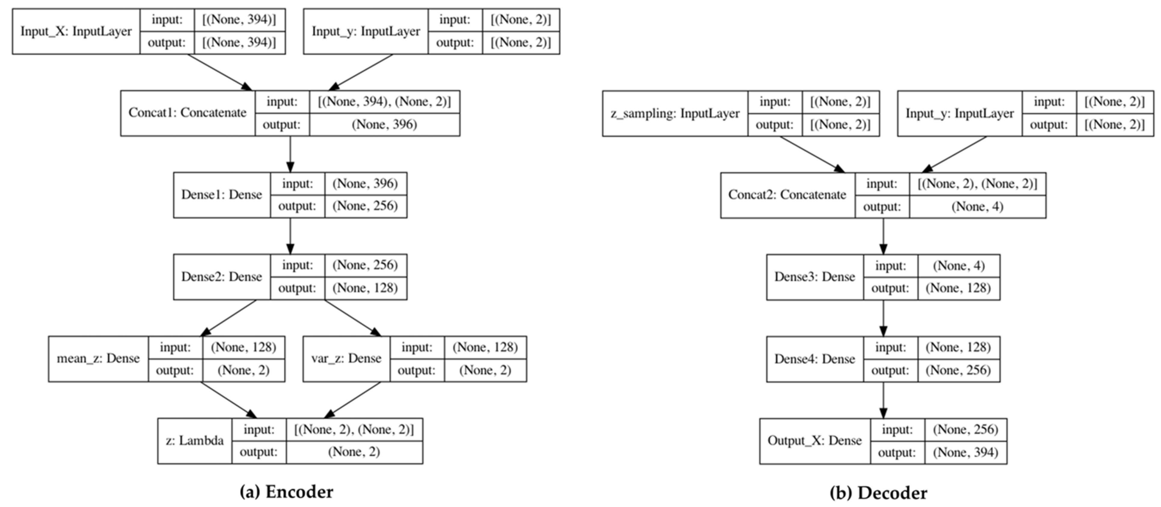
Appendix A describes the architecture of the generative model used in the experiment. We used Python 3.7.3 and TensorFlow 2.5.0, which is a deep learning framework, to implement C-VAE. Figure A1 shows the developed encoder and decoder of C-VAE. The encoder input data include 394 variables, and the labels are extracted from patent data. The input is the result of concatenating 10 quantitative indicators and a 384-dimensional text vector. The label is a binary class for the TM and is a two-dimensional vector obtained through one-hot encoding. The output of the encoder is a two-dimensional latent vector.
Figure A1.
Architecture of the generative model used in the experiment. (a) An encoder of the generative model receives 10 quantitative indicators and embedding vectors for 384-dimensional natural language and returns a 2-dimensional latent vector; (b) the decoder generates data.
Figure A1.
Architecture of the generative model used in the experiment. (a) An encoder of the generative model receives 10 quantitative indicators and embedding vectors for 384-dimensional natural language and returns a 2-dimensional latent vector; (b) the decoder generates data.

The input of the decoder is a vector that is concatenated with a latent vector and a one-hot encoded label. In this case, the latent vector can be replaced with a random number. In the model training process, the dropout rate for each layer was set to 0.2 to prevent overfitting. In addition, that batch size was 256, and the optimizer used root-mean-squared propagation.
Appendix B
Appendix B describes the process for determining the hyperparameter of the proposed method. First, we predicted the test data with a model trained only on raw data to determine the performance baseline. The performance measures used in the experiment were F1-score, Geometric Mean (GM), False Positive Rate (FPR), and Area Under the Curve (AUC). The measures were calculated as True Positive (TP), True Negative (TN), False Positive (FP), and False Negative (FN).
The F1-score is calculated as follows:
where Precision is TP/(TP + FP) and Recall is TP/(TP + FN). Furthermore, the FPR is FP/(FP + TN).
The GM is calculated as follows:
where the Specificity is TN/(TN/FP). AUC indicates the area of the Receiver Operating Characteristics (ROC) curve. For all measures, it is judged that the closer the value is to 1, the better the prediction performance.

Table A1.
Result of comparing the performance to determine the hyperparameter of the proposed method.
Table A1.
Result of comparing the performance to determine the hyperparameter of the proposed method.
| Results | Litigation | Valuation | Transfer | |||||||||
|---|---|---|---|---|---|---|---|---|---|---|---|---|
| F1-Score | GM | FPR | AUC | F1-Score | GM | FPR | AUC | F1-Score | GM | FPR | AUC | |
| Baseline | 0.000 | 0.000 | 0.000 | 0.500 | 0.229 | 0.372 | 0.009 | 0.565 | 0.336 | 0.473 | 0.051 | 0.593 |
| 0.066 | 0.493 | 0.075 | 0.594 | 0.404 | 0.675 | 0.118 | 0.699 | 0.452 | 0.621 | 0.188 | 0.644 | |
| 0.062 | 0.494 | 0.082 | 0.592 | 0.395 | 0.681 | 0.133 | 0.701 | 0.457 | 0.633 | 0.223 | 0.646 | |
| 0.065 | 0.515 | 0.085 | 0.602 | 0.385 | 0.681 | 0.144 | 0.699 | 0.458 | 0.637 | 0.243 | 0.647 | |
| 0.063 | 0.514 | 0.087 | 0.601 | 0.376 | 0.679 | 0.153 | 0.695 | 0.459 | 0.641 | 0.258 | 0.648 | |
| 0.062 | 0.513 | 0.090 | 0.600 | 0.372 | 0.679 | 0.159 | 0.695 | 0.463 | 0.646 | 0.272 | 0.651 | |
| 0.061 | 0.513 | 0.091 | 0.599 | 0.370 | 0.679 | 0.161 | 0.694 | 0.465 | 0.649 | 0.276 | 0.653 | |
Table A1 shows the results of a greedy search for several values to find the optimal value. The model’s performance may fluctuate due to the randomness of the generative model. Therefore, the measures used the average of the values obtained using a 10-fold cross-validation. The predictive model for predicting target variables is logistic regression. The model returns well-corrected predictions because it optimizes for log-loss. As a result, the performance improvement of the proposed method evidently increases as the label becomes imbalanced.
References
- Johnson, J.M.; Khoshgoftaar, T.M. Survey on deep learning with class imbalance. J. Big Data 2019, 6, 27. [Google Scholar] [CrossRef]
- Jiawei, H.; Micheline, K.; Jian, P. Data Mining: Concepts and Techniques, 3rd ed.; Elsevier: New York, NY, USA, 2012; ISBN 9780123814791. [Google Scholar]
- Ivanović, M.; Radovanović, M. Modern Machine Learning Techniques and Their Applications. In Electronics, Communications and Networks IV: Proceedings of the International Conference on Electronics, Communications and Networks, Beijing, China, 12–15 December 2014; CRC Press: London, UK, 2015. [Google Scholar]
- LeCun, Y.; Bengio, Y.; Hinton, G. Deep learning. Nature 2015, 521, 436–444. [Google Scholar] [CrossRef] [PubMed]
- Bojarski, M.; Del Testa, D.; Dworakowski, D.; Firner, B.; Flepp, B.; Goyal, P.; Jackel, L.D.; Monfort, M.; Muller, U.; Zhang, J.; et al. End to End Learning for Self-Driving Cars. arXiv 2016, arXiv:1604.07316. [Google Scholar]
- Van den Oord, A.; Dieleman, S.; Zen, H.; Simonyan, K.; Vinyals, O.; Graves, A.; Kalchbrenner, N.; Senior, A.; Kavukcuoglu, K. Wavenet: A Generative Model for Raw Audio. arXiv 2016, arXiv:1609.03499. [Google Scholar]
- Isola, P.; Zhu, J.-Y.; Zhou, T.; Efros, A.A. Image-to-Image Translation with Conditional Adversarial Networks. In Proceedings of the IEEE Conference on Computer Vision and Pattern Recognition (CVPR), Honolulu, HI, USA, 21–26 July 2017; pp. 1125–1134. [Google Scholar]
- Esteva, A.; Kuprel, B.; Novoa, R.A.; Ko, J.; Swetter, S.M.; Blau, H.M.; Thrun, S. Dermatologist-level classification of skin cancer with deep neural networks. Nature 2017, 542, 115–118. [Google Scholar] [CrossRef]
- Jiang, H.; Kim, B.; Guan, M.Y.; Gupta, M. To Trust or Not to Trust a Classifier. In Proceedings of the Advances in Neural Information Processing System, Montréal, QC, Canada, 4 December 2018. [Google Scholar]
- Janet, J.P.; Duan, C.; Yang, T.; Nandy, A.; Kulik, H.J. A quantitative uncertainty metric controls error in neural network-driven chemical discovery. Chem. Sci. 2019, 10, 7913–7922. [Google Scholar] [CrossRef]
- Malinin, A. Uncertainty Estimation in Deep Learning with Application to Spoken Language Assessment. Doctoral Dissertation, University of Cambridge, Cambridge, UK, 2019. [Google Scholar]
- Abdar, M.; Pourpanah, F.; Hussain, S.; Rezazadegan, D.; Liu, L.; Ghavamzadeh, M.; Fieguth, P.; Cao, X.; Khosravi, A.; Acharya, U.R.; et al. A review of uncertainty quantification in deep learning: Techniques, applications and challenges. Inf. Fusion 2021, 76, 243–297. [Google Scholar] [CrossRef]
- Hora, S.C. Aleatory and epistemic uncertainty in probability elicitation with an example from hazardous waste management. Reliab. Eng. Syst. Saf. 1996, 54, 217–223. [Google Scholar] [CrossRef]
- Der Kiureghian, A.; Ditlevsen, O. Aleatory or epistemic? Does it matter? Struct. Saf. 2009, 31, 105–112. [Google Scholar] [CrossRef]
- Hüllermeier, E.; Waegeman, W. Aleatoric and epistemic uncertainty in machine learning: An introduction to concepts and methods. Mach. Learn. 2021, 110, 457–506. [Google Scholar] [CrossRef]
- Kendall, A.; Gal, Y. What Uncertainties Do We Need in Bayesian Deep Learning for Computer Vision? In Proceedings of the Advances in Neural Information Processing System, Long Beach, CA, USA, 24 January 2018. [Google Scholar]
- Gneiting, T.; Balabdaoui, F.; Raftery, A.E. Probabilistic forecasts, calibration and sharpness. J. R. Stat. Soc. Ser. B (Stat. Methodol.) 2007, 69, 243–268. [Google Scholar] [CrossRef]
- Kleiber, W.; Raftery, A.E.; Gneiting, T. Geostatistical Model Averaging for Locally Calibrated Probabilistic Quantitative Precipitation Forecasting. J. Am. Stat. Assoc. 2011, 106, 1291–1303. [Google Scholar] [CrossRef]
- Minderer, M.; Djolonga, J.; Romijnders, R.; Hubis, F.; Zhai, X.; Houlsby, N.; Tran, D.; Lucic, M. Revisiting the Calibration of Modern Neural Networks. In Proceedings of the Advances in Neural Information Processing System, Online, 12 July 2021; Volume 34, pp. 15682–15694. [Google Scholar]
- Jagannatha, A.; Yu, H. Calibrating Structured Output Predictors for Natural Language Processing. In Proceedings of the Conference Association for Computational Linguistics Meeting, Online, 5–10 July 2020; pp. 2078–2092. [Google Scholar]
- Jiang, Z.; Araki, J.; Ding, H.; Neubig, G. How Can We Know When Language Models Know? On the Calibration of Language Models for Question Answering. Trans. Assoc. Comput. Linguist. 2021, 9, 962–977. [Google Scholar] [CrossRef]
- Zhang, S.; Gong, C.; Choi, E. Knowing More About Questions Can Help: Improving Calibration in Question Answering. arXiv 2021, arXiv:2106.01494. [Google Scholar] [CrossRef]
- Tekic, Z.; Kukolj, D. Threat of Litigation and Patent Value: What Technology Managers Should Know. Res. Technol. Manag. 2013, 56, 18–25. [Google Scholar] [CrossRef]
- Lee, J.; Kang, J.; Park, S.; Jang, D.; Lee, J. A Multi-Class Classification Model for Technology Evaluation. Sustainability 2020, 12, 6153. [Google Scholar] [CrossRef]
- Chien, C.V. Predicting Patent Litigation. Tex. L. Rev. 2011, 90, 283–329. [Google Scholar]
- Cowart, T.W.; Lirely, R.; Avery, S. Two Methodologies for Predicting Patent Litigation Outcomes: Logistic Regression Versus Classification Trees. Am. Bus. Law J. 2014, 51, 843–877. [Google Scholar] [CrossRef]
- Sokhansanj, B.A.; Rosen, G.L. Predicting Institution Outcomes for Inter Partes Review (IPR) Proceedings at the United States Patent Trial & Appeal Board by Deep Learning of Patent Owner Preliminary Response Briefs. Appl. Sci. 2022, 12, 3656. [Google Scholar] [CrossRef]
- Chung, P.; Sohn, S.Y. Early detection of valuable patents using a deep learning model: Case of semiconductor industry. Technol. Forecast. Soc. Chang. 2020, 158, 120146. [Google Scholar] [CrossRef]
- Trappey, A.J.C.; Trappey, C.V.; Govindarajan, U.H.; Sun, J.J.H. Patent Value Analysis Using Deep Learning Models—The Case of IoT Technology Mining for the Manufacturing Industry. IEEE Trans. Eng. Manag. 2019, 68, 1334–1346. [Google Scholar] [CrossRef]
- Da Silva, V.L.; Kovaleski, J.L.; Pagani, R.N. Technology Analysis & Strategic Management Technology Transfer in the Supply Chain Oriented to Industry 4.0: A Literature Review. Technol. Anal. Strateg. Manag. 2018, 31, 546–562. [Google Scholar] [CrossRef]
- Lee, J.; Lee, J.; Kang, J.; Kim, Y.; Jang, D.; Park, S. Multimodal Deep Learning for Patent Classification. In Proceedings of 6th International Congress on Information and Communication Technology, ICICT 2021, London, UK, 25–26 February 2021; Springer Science and Business Media Deutschland GmbH: Berlin, Germany, 2022; Volume 217, pp. 281–289. [Google Scholar]
- Kong, Q.; Zhao, H.; Lu, B.-L. Adaptive Ensemble Learning Strategy Using an Assistant Classifier for Large-Scale Imbalanced Patent Categorization. In Proceedings of the International Conference on Neural Information Processing; Springer: Berlin/Heidelberg, Germany, 2010; Volume 6443, pp. 601–608. [Google Scholar] [CrossRef]
- Platt, J. Probabilistic Outputs for Support Vector Machines and Comparisons to Regularized Likelihood Methods. Adv. Large Margin Classif. 1999, 10, 61–74. [Google Scholar]
- Guo, C.; Pleiss, G.; Sun, Y.; Weinberger, K.Q. On Calibration of Modern Neural Networks. In Proceedings of the International Conference on Machine Learning, PMLR, Sydney, Australia, 6 August 2017; pp. 1321–1330. [Google Scholar]
- Zadrozny, B.; Elkan, C. Obtaining Calibrated Probability Estimates from Decision Trees and Naive Bayesian Classifiers. In Proceedings of the ICML, Online, 28 June–1 July 2001; pp. 609–616. [Google Scholar]
- Naeini, M.P.; Cooper, G.; Hauskrecht, M. Obtaining Well Calibrated Probabilities Using Bayesian Binning. In Proceedings of the Twenty-Ninth AAAI Conference on Artificial Intelligence, Austin, TX, USA, 25–30 January 2015. [Google Scholar]
- Nixon, J.; Dusenberry, M.W.; Zhang, L.; Jerfel, G.; Tran, D. Measuring Calibration in Deep Learning. In Proceedings of the CVPR Workshops, Long Beach, CA, USA, 15 June 2019; pp. 38–41. [Google Scholar]
- Thulasidasan, S.; Chennupati, G.; Bilmes, J.; Bhattacharya, T.; Michalak, S.E. On Mixup Training: Improved Calibration and Predictive Uncertainty for Deep Neural Networks. In Proceedings of the Advances in Neural Information Processing System, Vancouver, BC, Canada, 13 December 2019. [Google Scholar] [CrossRef]
- Zhang, L.; Deng, Z.; Kawaguchi, K.; Zou, J. When and How Mixup Improves Calibration. In Proceedings of the 39th International Conference on Machine Learning, PMLR, Baltimore, MD, USA, 17–23 July 2022; pp. 26135–26160. [Google Scholar]
- Ovadia, Y.; Fertig, E.; Ren, J.; Nado, Z.; Sculley, D.; Nowozin, S.; Dillon, J.V.; Lakshminarayanan, B.; Snoek, J. Can You Trust Your Model’s Uncertainty? Evaluating Predictive Uncertainty Under Dataset Shift. In Proceedings of the Advances in Neural Information Processing System, Vancouver, BC, Canada, 13 December 2019. [Google Scholar]
- Chan, A.J.; Alaa, A.M.; Qian, Z.; van der Schaar, M. Unlabelled Data Improves Bayesian Uncertainty Calibration under Covariate Shift. In Proceedings of the 37th International Conference on Machine Learning, PMLR, Online, 13–18 July 2020; pp. 1392–1402. [Google Scholar]
- Hendrycks, D.; Gimpel, K. A Baseline for Detecting Misclassified and out-of-Distribution Examples in Neural Networks. arXiv 2016, arXiv:1610.02136. [Google Scholar]
- Pereyra, G.; Tucker, G.; Chorowski, J.; Kaiser, Ł.; Hinton, G. Regularizing Neural Networks by Penalizing Confident Output Distributions. arXiv 2017, arXiv:1701.06548. [Google Scholar]
- Krishnan, R.; Tickoo, O. Improving Model Calibration with Accuracy versus Uncertainty Optimization. In Proceedings of the Advances in Neural Information Processing System, Vancouver, BC, Canada, 6 December 2020; pp. 18237–18248. [Google Scholar]
- Jiang, X.; Deng, X. Knowledge Reverse Distillation Based Confidence Calibration for Deep Neural Networks. Neural Process. Lett. 2022, 1–16. [Google Scholar] [CrossRef]
- Xenopoulos, P.; Rulff, J.; Nonato, L.G.; Barr, B.; Silva, C. Calibrate: Interactive Analysis of Probabilistic Model Output. arXiv 2022, arXiv:2207.13770. [Google Scholar]
- Mukdasai, K.; Sabir, Z.; Raja, M.A.Z.; Sadat, R.; Ali, M.R.; Singkibud, P. A numerical simulation of the fractional order Leptospirosis model using the supervise neural network. Alex. Eng. J. 2022, 61, 12431–12441. [Google Scholar] [CrossRef]
- Liu, Q.; Wu, H.; Ye, Y.; Zhao, H.; Liu, C.; Du, D. Patent Litigation Prediction: A Convolutional Tensor Factorization Approach. In Proceedings of the International Joint Conference on Artificial Intelligence, Stockholm, Sweden, 13 July 2017; pp. 5052–5059. [Google Scholar]
- Kwon, O. A new ensemble method for gold mining problems: Predicting technology transfer. Electron. Commer. Res. Appl. 2012, 11, 117–128. [Google Scholar] [CrossRef]
- Kwon, O.; Lee, J.S. Smarter Classification for Imbalanced Data Set and Its Application to Patent Evaluation. J. Intell. Inf. Syst. 2014, 20, 15–34. [Google Scholar] [CrossRef]
- Setiawan, A.A.R.; Sulaswatty, A.; Haryono, A. Finding the Most Efficient Technology Transfer Route Using Dijkstra Algorithm to Foster Innovation: The Case of Essential Oil Developments in the Research Center for Chemistry at the Indonesian Institute of Sciences. STI Policy Manag. J. 2016, 1, 75–102. [Google Scholar] [CrossRef]
- Sohn, K.; Yan, X.; Lee, H. Learning Structured Output Representation Using Deep Conditional Generative Models. In Proceedings of the Advances in Neural Information Processing System, Montreal, QC, Canada, 7 December 2015. [Google Scholar]
- Lopez-Martin, M.; Carro, B.; Sanchez-Esguevillas, A.; Lloret, J. Conditional Variational Autoencoder for Prediction and Feature Recovery Applied to Intrusion Detection in IoT. Sensors 2017, 17, 1967. [Google Scholar] [CrossRef] [PubMed]
- Sweers, T. Autoencoding Credit Card Fraud. Bachelor’s Thesis, Radboud University, Nijmegen, The Netherlands, 2018. [Google Scholar]
- Andrei Fajardo, V.; Findlay, D.; Houmanfar, R.; Charu, C.; Jiaxi, L.; Xie, H. VOS: A Method for Variational Oversampling of Imbalanced Data Charu Jaiswal. arXiv 2018, arXiv:1809.02596. [Google Scholar]
- Xu, H.; Feng, Y.; Chen, J.; Wang, Z.; Qiao, H.; Chen, W.; Zhao, N.; Li, Z.; Bu, J.; Li, Z.; et al. Unsupervised Anomaly Detection via Variational Auto-Encoder for Seasonal KPIs in Web Applications. In Proceedings of the 2018 World Wide Web Conference, Lyon, France, 23–27 April 2018; pp. 187–196. [Google Scholar] [CrossRef]
- Lu, Y.; Xu, P. Anomaly Detection for Skin Disease Images Using Variational Autoencoder. arXiv 2018, arXiv:1807.01349. [Google Scholar]
- Urteaga, I.; Li, K.; Shea, A.; Vitzthum, V.J.; Wiggins, C.H.; Elhada, N. A Generative Modeling Approach to Calibrated Predictions: A Use Case on Menstrual Cycle Length Prediction Generative Modeling for Calibrated Predictions. In Proceedings of the Machine Learning for Healthcare Conference, Online, 6 August 2021; Volume 149, pp. 535–566. [Google Scholar]
- Han, P.K.J.; Klein, W.M.P.; Arora, N.K. Varieties of Uncertainty in Health Care: A Conceptual Taxonomy. Med. Decis. Mak. 2011, 31, 828–838. [Google Scholar] [CrossRef]
- Alba, A.C.; Agoritsas, T.; Walsh, M.; Hanna, S.; Iorio, A.; Devereaux, P.J.; McGinn, T.; Guyatt, G. Discrimination and Calibration of Clinical Prediction Models. JAMA 2017, 318, 1377–1384. [Google Scholar] [CrossRef] [PubMed]
- Rajkomar, A.; Oren, E.; Chen, K.; Dai, A.M.; Hajaj, N.; Hardt, M.; Liu, P.J.; Liu, X.; Marcus, J.; Sun, M.; et al. Scalable and accurate deep learning with electronic health records. NPJ Digit. Med. 2018, 1, 18. [Google Scholar] [CrossRef]
- Choi, J.; Moo Yi, K.; Kim, J.; Choo, J.; Kim, B.; Chang, J.; Gwon, Y.; Jin Chang, H. VaB-AL: Incorporating Class Imbalance and Difficulty with Variational Bayes for Active Learning. In Proceedings of the IEEE/CVF Conference on Computer Vision and Pattern Recognition, Nashville, TN, USA, 20–25 June 2021; pp. 6749–6758. [Google Scholar]
- Zhu, J.-Y.; Zhang, R.; Pathak, D.; Darrell, T.; Efros, A.A.; Wang, O.; Shechtman, E. Toward Multimodal Image-to-Image Translation. In Proceedings of the Advances in Neural Information Processing System, Long Beach, CA, USA, 4 December 2017. [Google Scholar]
- Tran, M.-N.; Nott, D.J.; Kohn, R. Variational Bayes with Intractable Likelihood. J. Comput. Graph. Stat. 2017, 26, 873–882. [Google Scholar] [CrossRef]
- Hwang, J.-T.; Kim, B.-K.; Jeong, E.-S. Patent Value and Survival of Patents. J. Open Innov. Technol. Mark. Complex. 2021, 7, 119. [Google Scholar] [CrossRef]
- Hoskins, J.D.; Carson, S.J. Industry conditions, market share, and the firm’s ability to derive business-line profitability from diverse technological portfolios. J. Bus. Res. 2022, 149, 178–192. [Google Scholar] [CrossRef]
- Ren, X.; Yang, T.; Wang, Y.; Zeng, W. Do generative models know disentanglement? contrastive learning is all you need. arXiv 2021, arXiv:2102.10543. [Google Scholar]
- Reimers, N.; Gurevych, I. Sentence-BERT: Sentence Embeddings using Siamese BERT-Networks. In Proceedings of the 2019 Conference on Empirical Methods in Natural Language Processing and the 9th International Joint Conference on Natural Language Processing (EMNLP-IJCNLP) 2019, Hong Kong, China, 3–7 November 2019; pp. 3973–3983. [Google Scholar]
- Menell, P.S. An Analysis of the Scope of Copyright Protection for Application Programs. Stanf. Law Rev. 1989, 41, 1045. [Google Scholar] [CrossRef]
- Cunningham, J.A.; O’Reilly, P. Macro, meso and micro perspectives of technology transfer. J. Technol. Transf. 2018, 43, 545–557. [Google Scholar] [CrossRef]
- Alexander, A.; Martin, D.P.; Manolchev, C.; Miller, K. University–industry collaboration: Using meta-rules to overcome barriers to knowledge transfer. J. Technol. Transf. 2018, 45, 371–392. [Google Scholar] [CrossRef]
- Xu, X.; Gui, M. Applying data mining techniques for technology prediction in new energy vehicle: A case study in China. Environ. Sci. Pollut. Res. 2021, 28, 68300–68317. [Google Scholar] [CrossRef] [PubMed]
- Peacock, J. Two-dimensional goodness-of-fit testing in astronomy. Mon. Not. R. Astron. Soc. 1983, 202, 615–627. [Google Scholar] [CrossRef]
- Fasano, G.; Franceschini, A. A multidimensional version of the Kolmogorov–Smirnov test. Mon. Not. R. Astron. Soc. 1987, 225, 155–170. [Google Scholar] [CrossRef]
Figure 1.
Architecture of the proposed methodology.

Figure 2.
Distribution of the prediction probability for the target variables (when the generative model was C-VAE and the predictors were quantitative indicators and text of documents). (a) This figure shows the distribution of the prediction probabilities when the target variable was Litigation, which shows that the overall likelihood increased when the proposed method was used; (b) predicted distribution when the target variable was Valuation: this figure shows that the probability increases by 0.4 or more; (c) predicted distribution when the target variable is Transfer: it shows a similar pattern to the distribution in (b).

Figure 3.
Results of comparing the confidence of the baseline and proposed methodology (when the generative model was C-VAE and the predictors were quantitative indicators and document texts). (a) As a result, the proposed method calibrated the confidence better than the baseline; (b) the proposed method calibrated the confidence better than the baseline; (c) the proposed method calibrated the confidence of transferred patents better than the baseline; (d) the difference between the mean of the confidence and the accuracy was smaller for the proposed method than the baseline; (e) confidence was calibrated better than confidence in Litigation cases; (f) confidence was calibrated better in Transfer cases than in other cases.

Figure 4.
Comparison of differences between the accuracy and likelihood. (a) When the generative model was C-VAE and document texts were used as a predictor, the difference was the smallest; (b) it was most suitable when C-VAE and document texts were used as in where the target variable was Litigation; (c) the difference was the smallest when the generative model was C-VAE and quantitative indicators and document texts were used as predictors.

Table 1.
Variables used in the proposed model.
| Variables | Description |
|---|---|
| claim | Number of claims |
| inventor | Number of inventors |
| ipc | Number of International Patent Classification (IPC) codes |
| cpc | Number of Cooperative Patent Classification (CPC) codes |
| citeP | Number of cited patents |
| citeC | Number of countries for cited patents |
| citeR | Number of cited non-patent documents |
| famP | Number of family patents |
| famC | Number of countries for family patents |
| famE | Number of European Patent Office family patents |
| Embp2 | Variables for text transformed into a pre-trained language model |
Table 2.
Results of statistical test for Hypothesis 1.
| Case | Statistics | Claim | Inventor | ipc | cpc | citeP | citeC | citeR | famP | famC | famE |
|---|---|---|---|---|---|---|---|---|---|---|---|
| Litigation | Avg. Y | 23.536 | 1.544 | 3.656 | 4.656 | 223.584 | 3.600 | 66.664 | 74.832 | 5.560 | 20.400 |
| Std. Y | 12.981 | 1.874 | 4.785 | 9.004 | 430.433 | 2.626 | 140.082 | 178.146 | 3.965 | 23.832 | |
| Avg. N | 18.168 | 1.680 | 3.128 | 3.880 | 69.560 | 2.408 | 8.288 | 3.960 | 32.928 | 8.216 | |
| Std. N | 10.662 | 1.831 | 2.558 | 4.705 | 390.268 | 2.113 | 34.262 | 3.275 | 150.234 | 9.228 | |
| Levene 1 | 0.204 | 0.747 | 0.114 | 0.396 | 0.007 | 0.001 | <0.001 | 0.090 | 0.002 | <0.001 | |
| t-test 2 | <0.001 | 0.564 | 0.280 | 0.396 | 0.003 | <0.001 | <0.001 | 0.046 | 0.001 | <0.001 | |
| Wilcoxon 3 | <0.001 | 0.360 | 0.784 | 0.405 | <0.001 | <0.001 | <0.001 | <0.001 | 0.001 | <0.001 | |
| KS-test 4 | 0.001 | 0.614 | 0.721 | 0.721 | <0.001 | <0.001 | <0.001 | <0.001 | <0.001 | <0.001 | |
| Valuation | Avg. Y | 23.442 | 2.280 | 3.892 | 5.738 | 239.252 | 4.127 | 52.799 | 169.694 | 7.078 | 23.140 |
| Std. Y | 16.621 | 2.847 | 5.096 | 11.006 | 562.636 | 3.048 | 117.259 | 415.457 | 4.455 | 29.686 | |
| Avg. N | 17.170 | 1.849 | 3.089 | 3.707 | 47.966 | 2.476 | 11.476 | 3.753 | 29.337 | 7.858 | |
| Std. N | 8.966 | 2.129 | 2.583 | 5.545 | 130.851 | 1.904 | 48.123 | 3.241 | 159.323 | 9.322 | |
| Levene | <0.001 | <0.001 | <0.001 | <0.001 | <0.001 | <0.001 | <0.001 | <0.001 | <0.001 | <0.001 | |
| t-test | <0.001 | <0.001 | <0.001 | <0.001 | <0.001 | <0.001 | <0.001 | <0.001 | <0.001 | <0.001 | |
| Wilcoxon | <0.001 | 0.292 | 0.337 | 0.812 | <0.001 | <0.001 | <0.001 | <0.001 | <0.001 | <0.001 | |
| KS-test | <0.001 | <0.001 | 0.053 | <0.001 | <0.001 | <0.001 | <0.001 | <0.001 | <0.001 | <0.001 | |
| Transfer | Avg. Y | 17.266 | 2.347 | 3.257 | 4.556 | 80.523 | 3.042 | 17.588 | 44.854 | 4.189 | 10.312 |
| Std. Y | 9.586 | 2.439 | 2.839 | 6.158 | 230.131 | 2.560 | 56.210 | 198.785 | 3.123 | 13.353 | |
| Avg. N | 18.190 | 1.819 | 3.139 | 3.727 | 61.215 | 2.519 | 13.444 | 3.870 | 38.910 | 8.814 | |
| Std. N | 11.348 | 2.184 | 2.937 | 5.484 | 225.695 | 1.917 | 56.539 | 3.493 | 197.317 | 12.343 | |
| Levene | 0.001 | <0.001 | 0.428 | <0.001 | 0.003 | <0.001 | 0.011 | 0.332 | 0.182 | 0.014 | |
| t-test | 0.001 | <0.001 | 0.140 | <0.001 | 0.002 | <0.001 | 0.008 | 0.276 | <0.001 | <0.001 | |
| Wilcoxon | 0.022 | <0.001 | 0.026 | <0.001 | 0.048 | <0.001 | <0.001 | <0.001 | <0.001 | <0.001 | |
| KS-test | 0.066 | <0.001 | 0.147 | <0.001 | 0.026 | <0.001 | <0.001 | <0.001 | <0.001 | <0.001 |
1 p-value of Levene’s test for homogeneity of variance. 2 p-value of t-test for homogeneity of average. 3 p-value of Wilcoxon Rank-Sum test, a nonparametric method for t-test. 4 p-value of Kolmogorov–Smirnov test for homogeneity of distribution.
Table 3.
Result of splitting the data to train the model.
| Dataset | Litigation | Valuation | Transfer | ||||||
|---|---|---|---|---|---|---|---|---|---|
| Y | N | Ratio (%) | Y | N | Ratio (%) | Y | N | Ratio (%) | |
| Raw data | 125 | 11,319 | 1.092 | 1162 | 10,282 | 10.154 | 2642 | 8802 | 23.086 |
| Training data | 61 | 5520 | 1.093 | 566 | 5015 | 10.142 | 1289 | 4292 | 23.096 |
| Validation data | 26 | 2388 | 1.077 | 245 | 2169 | 10.149 | 557 | 1857 | 23.074 |
| Test data | 38 | 3411 | 1.102 | 351 | 3098 | 10.177 | 796 | 2653 | 23.079 |
Table 4.
Results of statistical tests for Hypothesis 2.
| Generative Model | Predictors | Parameter | Litigation | Valuation | Transfer | |||
|---|---|---|---|---|---|---|---|---|
| Statistics | p-Value | Statistics | p-Value | Statistics | p-Value | |||
| VAE | Quant | 1 | 0.117 | 0.833 | 0.106 | 0.013 | 0.018 | >0.500 |
| 2 | 0.148 | >0.500 | 0.106 | 0.013 | 0.017 | >0.500 | ||
| 3 | 0.149 | >0.500 | 0.106 | 0.026 | 0.017 | >0.500 | ||
| Text | 0.141 | <0.001 | 0.071 | 0.210 | 0.045 | 0.339 | ||
| 0.141 | <0.001 | 0.075 | 0.157 | 0.038 | >0.500 | |||
| 0.141 | <0.001 | 0.114 | 0.010 | 0.056 | 0.321 | |||
| Quant + Text | 0.170 | 0.404 | 0.058 | 0.432 | 0.073 | 0.020 | ||
| 0.226 | 0.124 | 0.105 | 0.015 | 0.060 | 0.083 | |||
| 0.267 | 0.071 | 0.113 | 0.009 | 0.102 | 0.001 | |||
| C-VAE | Quant | 0.263 | 0.047 | 0.008 | >0.500 | 0.267 | <0.001 | |
| 0.308 | 0.012 | 0.012 | >0.500 | 0.259 | <0.001 | |||
| 0.308 | 0.018 | 0.014 | >0.500 | 0.277 | <0.001 | |||
| Text | 0.200 | 0.221 | 0.354 | <0.001 | 0.171 | <0.001 | ||
| 0.378 | 0.001 | 0.342 | <0.001 | 0.197 | <0.001 | |||
| 0.385 | 0.002 | 0.470 | <0.001 | 0.232 | <0.001 | |||
| Quant + Text | 0.646 | <0.001 | 0.421 | <0.001 | 0.156 | <0.001 | ||
| 0.588 | <0.001 | 0.177 | <0.001 | 0.155 | <0.001 | |||
| 0.635 | <0.001 | 0.428 | <0.001 | 0.156 | <0.001 | |||
Table 5.
Results of statistical tests for Hypothesis 3.
| Case | Performance Measure | Statistical Test | ||||
|---|---|---|---|---|---|---|
| Avg_Baseline | F1-Score | KS-Test 1 | Paired t-Test 2 | Wilcoxon 3 | ||
| Litigation | 0.010 | 0.040 | 0.065 | <0.001 | <0.001 | <0.001 |
| Valuation | 0.157 | 0.353 | 0.395 | <0.001 | <0.001 | <0.001 |
| Transfer | 0.286 | 0.445 | 0.465 | <0.001 | <0.001 | <0.001 |
1 KS test for the two-sided test with log-likelihood. 2 Paired t-test for one-sided test with log-likelihood. 3 Wilcoxon Signed Rank one-sided test. The null hypotheses for the one and two-sided tests are “the two distributions are equal” and “the log-likelihood is lower than before”, respectively.
Publisher’s Note: MDPI stays neutral with regard to jurisdictional claims in published maps and institutional affiliations. |
© 2022 by the authors. Licensee MDPI, Basel, Switzerland. This article is an open access article distributed under the terms and conditions of the Creative Commons Attribution (CC BY) license (https://creativecommons.org/licenses/by/4.0/).
Share and Cite
MDPI and ACS Style
Lee, J.; Park, S. A Study on the Calibrated Confidence of Text Classification Using a Variational Bayes. Appl. Sci. 2022, 12, 9007. https://doi.org/10.3390/app12189007
AMA Style
Lee J, Park S. A Study on the Calibrated Confidence of Text Classification Using a Variational Bayes. Applied Sciences. 2022; 12(18):9007. https://doi.org/10.3390/app12189007
Chicago/Turabian StyleLee, Juhyun, and Sangsung Park. 2022. "A Study on the Calibrated Confidence of Text Classification Using a Variational Bayes" Applied Sciences 12, no. 18: 9007. https://doi.org/10.3390/app12189007
Note that from the first issue of 2016, this journal uses article numbers instead of page numbers. See further details here.