
A Review of Road Surface Anomaly Detection and Classification Systems Based on Vibration-Based Techniques

Tecnologico de Monterrey, School of Engineering and Sciences, Mexico City 14380, Mexico
*
Author to whom correspondence should be addressed.
Appl. Sci. 2022, 12(19), 9413; https://doi.org/10.3390/app12199413
Submission received: 7 September 2022
/
Revised: 15 September 2022
/
Accepted: 15 September 2022
/
Published: 20 September 2022
(This article belongs to the Special Issue Applications of Artificial Intelligence to Improve Road Traffic Performance)
Abstract
:Road surfaces suffer from sources of deterioration, such as weather conditions, constant usage, loads, and the age of the infrastructure. These sources of decay generate anomalies that could cause harm to vehicle users and pedestrians and also develop a high cost to repair the irregularities. These drawbacks have motivated the development of systems that automatically detect and classify road anomalies. This study presents a narrative review focused on road surface anomaly detection and classification based on vibration-based techniques. Three methodologies were surveyed: threshold-based methods, feature extraction techniques, and deep learning techniques. Furthermore, datasets, signals, preprocessing steps, and feature extraction techniques are also presented. The results of this review show that road surface anomaly detection and classification performed through vibration-based methods have achieved relatively high performance. However, there are challenges related to the reproduction and heterogeneity of the results that have been reported that are influenced by the limited testing conditions, sample size, and lack of publicly available datasets. Finally, there is potential to standardize the features computed through the time or frequency domains and evaluate and compare the diverse set of settings of time-frequency methods used for feature extraction and signal representation.
1. Introduction
Road surface anomalies, such as potholes, cracks, rutting, or speed bumps deterioration, result from the constant usage, traffic loads, weather conditions, and age of the infrastructure and materials used in the construction of the roads [1,2]. These anomalies can be referred to as any deviation or variation from standard road conditions [3]. Furthermore, road defects have financial costs for governments to constantly maintain the road and keep it in good condition [4]. Moreover, it is crucial to attend to and monitor the road pavement condition due to the potential harm or accidents that could inflict on the vehicle users and pedestrians, its impact on fuel consumption, and the potential vehicle damage that these irregularities could inflict [5]. In addition, according to the World Bank, the density of paved roads in an optimal state can be used as an indicator of the economic strength and competitiveness of a country [6,7]. These factors make monitoring and maintaining the road in an optimal condition a crucial task for governments [8].
The traditional approach to monitoring and maintaining the road’s optimal condition is to employ Pavement Condition Index (PCI) surveys that are based on human observations. These surveys have been used by international road and highway technicians as a reference to diagnose road anomalies [9]. The roughness of the road surface is another crucial indicator used to assess the quality of roads and detect cracks and bumps [10,11]. However, in the case of PCI surveys, they are prone to subjective evaluation by the technician and can put the health of road operators at risk [12]. Otherwise, visual inspection methods are time-consuming and prone to human errors [13]. Thus, to counter the disadvantages of traditional approaches to evaluating the condition of roads, the literature has proposed developing systems that can automatically detect and classify these defects. There is great interest in developing these systems due to the potential impact they could have on intelligent transportation systems [14] and advanced driver assistance systems [15].
The systems developed in the literature for road surface anomaly detection and classification can be divided into vision-based, vibration-based, and 3D-reconstruction-based techniques [16]. Vision-based techniques use images to determine the presence of road anomalies through image processing and deep learning algorithms. On the other hand, the vibration-based techniques mainly employed inertial sensor measurements to detect and classify the presence of road anomalies. Finally, 3D-based reconstruction methods use stereo-vision technology to recognize and characterize the presence of road surface defects. The main goal of road surface anomaly detection and classification systems is to generate robust platforms that can provide information on the quality of the roads and warn of potential hazards [17].
A summary of the advantages and disadvantages of these systems can be appreciated in Table 1. As can be seen, vibration-based techniques have the main advantage of being the most cost-effective of the three methods since data are usually collected from smartphones [18]. However, this system requires the driver to pass over the anomaly to detect and characterize it since it relies on the measurements of inertial sensors such as gyroscopes and accelerometers. In the case of vision-based methods, they can detect the anomaly without passing over the anomaly. However, it is susceptible to lightning and shadow conditions. Finally, 3D reconstruction techniques can model the anomaly more precisely; nevertheless, it is a more expensive method [16].
Vibration-based techniques for road surface anomaly detection and classification have gained popularity due to the cost-effectiveness of this type of system. Inertial sensors (i.e., accelerometers and gyroscope sensors) commonly used for developing these systems can be easily embedded and used through smartphones [19]. However, as pointed out previously, some disadvantages mitigate its use, such as different sensor properties, smartphone or sensor placement within the vehicle, and diverse vehicle mechanical characteristics [11]. Hence, the above drawbacks have the potential to be addressed with further research.
Previous studies have made literature reviews or surveys focused on road surface anomaly detection. For example, Kim et al. [16] reviewed pothole detection methods in which vibration, vision, and 3D reconstruction methods were discussed and compared. Dib et al. [20] also presented a similar review in which the strengths and limitations of deep learning techniques and non-deep learning techniques for detecting damaged road surfaces are presented. Furthermore, in Dib’s study, vision-based procedures are extensively reviewed using deep learning techniques and non-deep learning technologies. However, vibration-based technologies have been reviewed to a lesser extent. Sattar et al. [10] present a literature review focused on detecting anomalies through smartphone sensors, such as accelerometer and gyroscope data, with particular attention to the threshold, machine learning, and dynamic time warping methods. However, no review has been conducted that presents a deeper explanation of vibration-based techniques for road surface anomaly detection and classification that expands on the feature engineering methods that have been used and the areas of opportunity that can be fulfilled to improve the performance of learning-based techniques.
This narrative literature review aims to provide a detailed presentation and discussion of approaches based on the vibration-based methods used to detect and classify anomalies on the road surface. The proposed categorization of vibration-based techniques is based on threshold, feature extraction, and deep learning techniques. A review of the datasets, sensors, preprocessing steps, and feature engineering methods (i.e., time analysis, frequency analysis, and time-frequency analysis) is also provided. The remainder of this study is organized as follows. Section 2 presents the search strategy used in the present narrative literature review. Section 3 presents the background of road anomaly detection and classification based on vibration-based techniques. Section 4 presents the datasets, sensors, and the preprocessing steps used for road surface anomaly detection and classification. Furthermore, Section 5 shows a detailed presentation of the feature extraction techniques commonly used to detect and classify road surface anomalies using machine learning or deep learning techniques. The discussion of the results of this literature review is presented in Section 6. Finally, Section 7 presents the findings of this study and future research directions.
2. Search Methodology
The narrative review presented in this study was primarily performed through the Web of Science and, to a lesser extent, with the help of Google Scholar databases. The search focused on conference and journal articles published from 2018 to 2022. The list of keywords used to perform this search was as follows:
- Road anomaly;
- Detection;
- Vibration;
- Machine Learning.
The articles were classified into three categories defined as threshold-based techniques, feature extraction with machine learning techniques, and deep learning techniques. The studies collected for this search mainly used acceleration and gyroscope data to detect and classify road anomalies or conditions. Figure 1 depicts the flow of activities in which the searching process was performed for this review. The information extracted from each study was focused on the year of publication, the author, the methodology, algorithms, and the preprocessing steps. In addition, special attention was given to the feature engineering methods that each author proposed. Therefore, this review is not focused on methods based on image processing or 3D reconstruction techniques since Kim et al. [16] presents an extensive review that covers them. However, specific articles selected for this survey were added when the authors compared or used vision-based and vibration-based techniques to develop their studies. The following sections present the main findings from this search and their respective discussion.
3. Road Anomaly Detection and Classification Approaches through Vibration-Based Techniques
Vibration-based techniques to detect and classify road anomalies can be categorized into three approaches [17]. The first is threshold-based methods, the second is learning-based techniques employing feature extraction before the learning stage, and machine learning techniques without feature extraction, such as deep learning algorithms [1]. Figure 2 shows an overview of the road anomaly detection and classification approaches based on vibrations collected from accelerometer and gyroscope data. As depicted in Figure 2, threshold techniques do not require a training process however an empirical calibration is needed before the validation. In the feature extraction and deep learning approaches, a step of model generation is performed through the training process and, consequently, a validation stage is performed. This section provides a brief overview and examples of these approaches and the authors’ reported methods and results.
In the case of the threshold-based methods, the metrics commonly reported are the true positives and false positives [21]. However, other metrics, such as the F1-score or the area under the receiver operating characteristic (ROC), have been reported [22,23]. On the other hand, the learning-based techniques with feature extraction or deep learning approaches are commonly evaluated through the accuracy and the metrics derived from the confusion matrix (i.e., recall, precision, and F1-score). Figure 3 shows a confusion matrix illustration along with the metrics derived from it, and Table 2 shows a summary of commonly reported validation metrics used to evaluate algorithms for detecting and classifying road surface anomalies based on vibration-based methods.
The accuracy represents the proportion of correctly identified observations among all the observations tested. The sensitivity indicates the percent of real positive cases accurately recognized, whereas specificity is the proportion of real negative data points accurately classified. The sensitivity and specificity are used to determine a classification model’s individual class performance. Otherwise, precision is defined as the ratio of true positives to true positives plus false positives. The F1-score value is calculated using the recall and precision parameters as shown in Table 2. Its value ranges from 0 to 1, with 0 indicating a poor forecast and 1 indicating a good forecast [25]. The F1-score is used to compare the performance across models.
3.1. Threshold-Based Methods
Threshold-based methods try to detect and classify road anomalies when a change in the amplitude, root mean square, or crest factor of the signal acquired from inertial sensors exceeds a certain predefined value [26]. Regarding this type of methodology, early studies, such as that of Astarita et al. [27] proposed to detect potholes and speed bumps by analyzing the extreme peaks of the z-axis of accelerometer data where the accuracy in detecting the speed bump was 90%, and the detection rate of potholes was 65%. Rishiwal et al. [28] proposed a threshold approach based on the analysis of the z-axis of the accelerometer data to measure the severity of bumps and potholes into three levels average severity, high severity, and very high severity. The thresholds were set empirically, and the method reported an accuracy of 93.75%.
In addition, Nguyen et al. [22] applied the Grubbs test on a sliding window to improve the threshold methods initially proposed by Mednis et al. [29]. These algorithms were the Z-THRESH, Z-DIFF, STDEV(Z), and G-ZERO. Z-THRESH aims to identify the anomaly if the amplitude of the z-axis of the accelerometer exceeds a specific value. Z-DIFF detects the anomaly if the difference between two successive measurements is more significant than a specific value. Furthermore, STDEV(Z) is related to the standard deviation of the sliding window; if the standard deviation surpasses a specific threshold, the anomaly is recognized. Finally, G-ZERO identifies the anomaly if the values in the three axes of the accelerometer are below a particular value [22,29]. Carlos et al. [14] also evaluated the thresholds proposed by Mednis’s study; his analysis showed that STDEV(Z) achieved the best results compared to G-ZERO, Z-DIFF, Z-THRESH, and support vector machines in terms of sensitivity, precision, and F1-score.
Other studies have also explored the combination of threshold-based techniques with learning-based techniques. For instance, Zheng et al. [21] proposed a threshold technique to identify where there might be an anomaly with a sliding window method. From this first detection, a random forest was used to filter out the window segments been actually normal from the segments that had anomalies. Finally, dynamic time wrapping classified the set of identified anomalies into potholes, speed bumps, and metal pumps. Sattar et al. [11] presented a similar approach, which consisted of employing the threshold method proposed by Yi et al. [30] and a Gaussian Mixture Model (GMM) to detect the road surface anomaly.
Finally, in Ref. [23], a querying-based road anomaly detection algorithm is proposed that takes advantage of self-similarity. This algorithm consists of two stages: first, the road anomaly is extracted by matching it with existing labeled anomalies; second, a re-comparison is made on suspicious road anomalies to classify the type of road anomaly (i.e., potholes, speed bumps, and metal pumps). The query algorithm is based on threshold values. A summary of the reference studies that have used threshold algorithms and their performance is presented in Table 3.
Based on the referred studies, it is appreciated that threshold-based techniques can achieve relatively high accuracy. In addition, it can be possible to combine threshold and machine learning techniques to improve or make a more robust algorithm. However, this method may require calibration since the threshold values are set empirically and may lack reproducibility, as pointed out by Li et al. [31]. In addition, thresholds are susceptible to noise and can only detect a single anomaly [22,32]. Therefore, the technique’s usefulness in different road scenarios could lead to underperformance in the detection and classification capability of the algorithms. However, the above could potentially be countered with dynamic thresholds instead of only a static threshold, as suggested in Ref. [10].
3.2. Learning-Based and Feature Extraction Methods
Some studies have opted to extract features from the accelerometer or gyroscope data by extracting features in the time-domain or frequency-domain (i.e., transforming the signal through the Fourier Transform (FT)) for road surface anomaly detection and classification. The above is done to input the extracted features into machine learning techniques. Figure 4 shows the flow of activities to apply learning-based techniques [33]. The first step consists in collecting the dataset. The second step is related to the preprocessing steps performed on the dataset, such as outliers detection, missing values handling, sensor data reorientation, re-sampling, and segmentation. The third step is related to the feature extraction process performed on the data. Finally, the last steps are related to the model generation and validation stages. In these two last stages, there is an iterative process in which different models are tested and validated since it is complicated to find a priori a model that represents all reality according to the No Free Lunch theorem [34].
Examples of studies that have performed this process are shown next. For instance, in Ref. [35], the data from accelerometers were used to identify potholes, speed bumps, straight roads, and curve roads by employing the power spectrum of the signal using the Fast Fourier Transform (FFT). In this case, the learning was completed with a k-nearest neighbor (KNN) and a multilayer perceptron with four hidden layers. The authors reported an accuracy of 95.55% for the KNN and 96.79% for the multilayer perceptron. Additionally, Celaya et al. [5] proposed to extract features from accelerometric data, such as the mean, variance, standard deviation, skewness, kurtosis, the minimum value, the maximum value, and dynamic range to detect speed bumps. The results of this study reported an accuracy of 97.14% by employing a logistic regression and finding the optimal coefficients of the logistic model through a genetic algorithm.
Similar research was conducted by Ferjani et al. [18], who explored the features of the time and frequency domains for road monitoring by testing a support vector machine, a decision tree, and a multilayer perceptron. The time-domain features were the mean, variance, standard deviation, integral square, root mean square, median, entropy, and range. The tested frequency-domain features were the spectrum energy, median frequency, mean power peak magnitude, minimum magnitude, and total power. Additionally, the authors tested the wavelet transform through a Daubechies 2 wavelet. Wu et al. [26] presented a similar feature extraction process that also proposed to extract features in the time, frequency, and time-frequency domain representations. The extracted features in the time-domain and frequency-domain were used to train a random forest classifier that achieved an accuracy of 95.7%, a precision of 88.5%, and a recall of 75.00%. In addition, Chen et al. [32] proposed to compute scale-invariant features from accelerometer signals. The methodology of this study was first to segment the road anomaly using a piecewise aggregate approximation method and then classify the anomaly by learning scale-invariant features by computing shapelets.
Anaissi et al. [36] worked with the vertical and lateral acceleration data to assess the condition of the road. The justification for working with the vertical and lateral data is to generate a system that can distinguish between benign anomalies and defects on the road. The features computed to generate the detection algorithm were the coefficient of variation applied to the vertical acceleration component. A second feature was to use the singular value decomposition and the coefficient of variation but applied to the lateral acceleration component. The classification was made with two one-class support vector machines with a reported accuracy of 97.5%. Similar to other studies reported in the literature, Zhou et al. [37] proposed to compute time and frequency domain features from both the accelerometer and gyroscope data and apply a support vector machine to classify the quality of manholes into three classes labeled as good, average, and poor. These labels represent the degree of subsidence; this study reported a mean accuracy of 84.40%. Furthermore, in Ref. [38], the authors proposed to detect surface road environments, such as cobblestones, flatlands, and transits, with a KNN and eight features derived from linear accelerations from the z and y axes and gyroscope data (i.e., roll and pitch angles) achieving an accuracy of 93.2%. Table 4 shows a summary of the studies that have used feature extraction and machine learning for road surface anomaly recognition and the performance reported in each reference work.
One of the critical advantages of learning-based techniques in combination with feature extraction is that the computational cost can be lower since no transformation is required, as in the case of time-domain features. However, the feature extraction could vary depending on the representation or domain in which the features are extracted or which statistics are computed, as presented in Ref. [26]. Furthermore, it is complicated to know a priori whether the set of proposed features could be invariant between samples and also assure class discrimination. The above was also pointed out in Ref. [18].
According to Chen et al. [32], one of the main drawbacks of time-domain and frequency-domain features is that the differences related to different classes of road anomalies are attributed to local signal segments rather than global features. This problem can be attributed to the noise and outliers present in the signal segments or due to shifting or scaling. The problem of shifting and scaling could also be counter with convolutional neural networks (CNNs) due to their ability to create invariant representations to translations and scaling from the input data [39]. This type of architecture used for vibration-based road surface anomaly detection and classification is presented in the next section.
3.3. Deep Learning-Based Methods
Deep learning techniques that have been used for road surface anomaly detection and classification are deep feedforward networks (DFN), CNNs, recurrent neural networks (RNNs), and long-short term memories (LSTMs) neural networks. These techniques have the main advantage of not requiring a feature engineering process since the algorithms can handle the raw data without needing any signal transformation or representation. Hence, the methodology presented in Figure 4 does not have a separate feature extraction stage since this process is performed during the model generation stage. For example, Varona et al. [1] proposed to automatically identify potholes and destabilizations produced by speed bumps or driver actions by comparing CNNs and LSTMs by processing the accelerometer data from smartphones. Baldini et al. [40] proposed to use time-frequency representations from inertial sensors to train CNNs to detect and classify road anomalies reporting an accuracy of 97.2%. The time-frequency representations tested were the short-time Fourier Transform (STFT) and the continuous wavelet transform (CWT). In addition, Luo et al. [3] compared DFNs, CNNs, and RNNs to identify eight pavement anomalies based on processing inertial sensors, spindle, and shock signals. This study showed that the RNNs performed better than the DFNs and CNNs with fewer parameters. Furthermore, Tiwari et al. [41] proposed a CNN for the road surface quality assessment and considered it as input accelerometer data. The proposal achieved a performance of 98.5% in terms of precision compared to neural feedforward networks and support vector machines.
Other studies have aimed to compare feature extraction approaches with deep learning techniques. An example is the one presented by Basavaraju et al. [42] that compared the use of decision trees and support vector machines with features extracted from accelerometer and gyroscope data with the input of raw data into a multilayer perceptron architecture to detect and classify smooth roads, potholes, and deep transverse cracks. The previous study used the three axes of the sensors instead of using only one single axis of the data, such as previous works [29]. Likewise, Menegazzo et al. [43] used inertial sensor datasets collected in different contexts to detect and classify surface road anomalies, such as dirt, cobblestone, and asphalt roads, by comparing classical machine learning techniques and deep learning techniques. Based on the results reported by the authors, it was observed that a CNN achieved the best performance with an accuracy of 93.17% compared to an LSTM and a gate recurrent unit. Finally, the study of Agebure et al. [44] developed a system focused on detecting road anomalies and determining the classification of unpaved road types. The algorithm used to perform the detection was a Spiking Neural Network originally proposed by Yellakour et al. [45] that, according to the authors, achieved a better performance than support vector machines and multilayer perceptrons. Table 5 shows a summary of the studies that have employed deep learning algorithms for road surface anomaly detection and classification, along with their performance.
Although deep learning techniques can automatically extract features from raw accelerometer data and achieve relatively high performance, as depicted in the mentioned studies, typical disadvantages of deep learning techniques exist. For example, the need for large sample size, high computational power requirements, the black-box structure of these classifiers that limits their interpretability and the setting process of its parameters could be considered an art [46,47].
4. Datasets and Signals
In this section, the datasets that have been used in the literature for road anomaly detection and classification based on vibration techniques are presented. Moreover, the sensors and preprocessing steps performed before the threshold or learning stage are shown.
4.1. Datasets
Regarding the datasets used for road surface anomaly detection and classification, authors have decided to generate or employ real datasets or generated datasets through simulation environments. For instance, Ferjani et al. [18] use the Pothole Lab dataset introduced in Ref. [14] to generate a simulated dataset for road anomaly detection and classification. Another dataset that was used in this study is the Gonzalez et al. [17] dataset; this is one of the few datasets that are publicly available, which facilitates the reproducibility and comparison of the methodologies, algorithms, and results. Chen et al. [32] also employed the datasets mentioned earlier in his study.
One of the major drawbacks in the current state of the art is that the study must be limited to describing the methodology or algorithm proposed and the experimental settings of the data collection process. However, the dataset in most cases is not available by the authors, which limits the potential reproducibility of the studies and, consequently, the validation of the algorithms or methodologies. The above is crucial for learning-based techniques since they depend on the sampled data to provide a performance metric that allows a homogeneous comparison. Examples of studies without publicly available datasets are Refs. [1,2,3,4,5,8,35,37,38].
4.2. Signals
This section presents an overview of the type of signals employed for road surface anomaly detection and classification. Moreover, the frequent preprocessing steps that have been applied to these signals before feature extraction or model generation stages are also presented. Finally, Table 6 shows a summary of the previously mentioned studies with the corresponding analyzed signals in each study.
4.2.1. Accelerometer Data
As pointed out, one common signal for road anomaly detection and classification is obtained through an accelerometer. An accelerometer is a device that measures the acceleration in an object (e.g., a vehicle, rocket, or aircraft) relative to the g-force. The output measurements of these devices can be viewed as a time series sampled at a specific frequency. This time series varies along time due to the movements of the analyzed object, which in the context of road anomaly detection will be the vehicle in a three-dimensional space [48]. When accelerometers are used for detecting and classifying road anomalies, it is expected that vehicle acceleration in different directions varies when the vehicle passes through the anomaly. This variation is sampled by the accelerometer embedded in smartphones [21]. One key factor that needs to be considered before working with accelerometer data is the minimum sampling frequency required to obtain a reliable time-domain representation of the signal and avoid aliasing problems. In this regard, the literature concerning a specific sampling rate is not concrete. For instance, in Ref. [49] a 50 Hz sampling frequency was chosen; however, other authors have worked with 95 or 100 Hz [5,37,43]. The selection of an adequate sampling rate is crucial to have a correct signal representation following the Nyquist criterion [50] and to realize a correct signal transformation and analysis through the use of either the FT or wavelet transform. The above also requires real-time embedded systems to assure a deterministic sampling procedure.
Despite their relatively easy use, accelerometer sensors have certain disadvantages that are essential to point out related to the noisy nature of the signals generated from these devices. This noisy nature difficulties road anomaly detection and classification since the feature extraction process could be complicated and, in some cases, even impossible [48]. To remove the low-frequency noise from the acceleration signals, what has been proposed is to use high-pass filters, such as Butterworth filters as proposed by Basavaraju et al. [42] and Wu et al. [26]. The above authors, in particular, proposed to use 11th-order Butterworth high-pass filters. Moreover, discrete wavelet transform (DWT) has been used for denoising acceleration and gyroscope signals, as proposed in the study of Zhou et al. [37]. Wakeel et al. [8] proposed to use the wavelet packet denoising technique to accelerometer and gyroscope data collected from a smartphone for road condition monitoring.
In addition, while working with accelerometer data, it is necessary to apply a reorientation process of the accelerometer’s coordinate system into the vehicle’s coordinate system [26]. The above can be achieved with the use of Euler angles [51]. Leonhard Euler introduced in his rotation theorem that any rotation can be described by employing only three angles. The rotations of a rigid object can be expressed in terms of rotation matrices labeled as D, C, and B; consequently, the general rotation A can be expressed as shown in Equation (1). Euler angles are the three angles that provide the three rotation matrices [52] established in Equation (1).
One component of accelerometers commonly analyzed for road anomaly detection is the z-axis, which is related to the vehicle’s vertical acceleration. However, other authors have also proposed to work with the other two axes to improve the performance of detection systems as proposed by Anaissi et al. [36]. Table 6 shows a detailed overview of the accelerometer and gyroscope axes analyzed in the literature for road surface anomaly detection and classification.
4.2.2. Gyroscope Data
Another type of sensor used for road surface anomaly detection and classification but to a lesser extent is the gyroscope. These devices can sense the angular velocity of an object when they are mounted on a frame while it is rotating. Several gyroscopes can be embedded in gyrocompass, inertial navigation systems, or inertial measurement units [53]. Like the accelerometer, an adequate preprocessing (i.e., correct sampling frequency and filtering) stage is needed to use this type of sensor for road surface anomaly detection and classification. Some of the studies that have used gyroscope data are the ones of Baldini et al. [40] that only study the y-axis of this device. Furthermore, similar to the accelerometer data, a reorientation process from the smartphone coordinate system to the vehicle coordinate system needs to be performed on the gyroscope data with the help of the Euler angles [42]. Despite that, gyroscopes have less use for road surface anomaly detection and classification, as depicted in Table 6, linear acceleration estimations can be computed through gyroscope and accelerator sensor data, as pointed out in Refs. [10,11]. Hence, its use in combination with other sensor readings could potentially improve the performance of road surface anomaly detection and classification systems.
5. Feature Extraction
This section describes and defines the computed features from both accelerometer and gyroscope data proposed in the literature. These features can be divided into time-domain, frequency-domain, and time-frequency domain features. Figure 5 shows an overview of the analysis techniques and features employed.
5.1. Time-Domain Features
Time-domain features are computed based on the signal amplitude that changes with time. Often these types of features are used to maintain low computational complexity. Moreover, this type of analysis often does not require additional signal transformation. Within the time-domain features, the magnitude of the accelerometer and gyroscope data are some of the commonly computed features. The reason to compute the magnitude is to remove the sensor data’s negative effects and reduce the variability imposed on the dataset due to the placement and inclination of the inertial sensor within the vehicle [37]. The magnitude calculation of the accelerometer data is shown in Equation (2) and for the gyroscope data in Equation (3) as proposed by Zhou et al. [37]. In Equation (3), , , and represent the triaxial accelerometer components while is the magnitude of the accelerometer signal. On the other hand, in Equation (3), , , and , are the triaxial angular velocities, and is the magnitude of the gyroscope signal.
Commonly computed statistics extracted from the accelerometer signal in the time-domain are the mean, variance, standard deviation, skewness, kurtosis, the maximum value, and dynamic range [54]. Table 7 shows the expression that allows computing the above features. In the expressions shown in Table 7, n represents the signal’s length or the window’s length, and is one single sample of the signal.
Other types of computed features in the time-domain are the mode, median, range, and root-mean-square, also used by Zhou et al. [37]. Another technique used for feature extraction is to compute the autocorrelation (i.e., the degree of similarity between the signal and a lagged version of itself [55]). The autocorrelation was proposed in the study of Wu et al. [26] for feature extraction of the z-axis of the accelerometer. The computation of these features requires that a signal window is measured. Thus, it is required that the anomaly is within that measured window. There is no exact methodology to select the correct window length of the signal; hence, a common approach is to test the system with different window lengths and select the one that produces the best performance, as suggested in the study of Menegazzo et al. [43].
In the same way, another type of characteristics that are commonly computed in what refers to the classification of signals are those obtained through different representations. For example, that is the representation in frequency and the time-frequency representations. These techniques will be introduced in the next sections.
5.2. Frequency-Domain Features
This section presents the background of Fourier analysis techniques used for feature extraction for road surface anomaly detection and classification. Moreover, the studies that used this signal representation are presented and analyzed. Additionally, the common features that have been computed based on the FT are also listed.
The FT is the technique used to generate a frequency representation of a signal defined in the time-domain. The FT’s basic concept is to create an orthogonal basis of sine and cosine functions with increasing frequency. The mathematical representation of the FT can be appreciated in the equation below [57].
where is a time-domain function multiplied with a complex exponential of frequency omega () that corresponds to the term . Nonetheless, the FT on discrete data vectors must be defined when computing or operating with real data. The Discrete Fourier Transform (DFT) is a discretized Fourier sequence for data vectors. For this purpose, the mathematical representation of the DFT is presented below.
The DFT is practical to approximate and compute the FT of data vectors, but it does not perform well with huge data vectors since the computational complexity increases. In this case, the computational complexity of the DFT is . The FFT was developed to reduce the computational complexity of the DFT. The FFT scales the computational complexity of the DFT to the order of . As N becomes very large, the component grows slowly, and the algorithm approaches linear scaling [58].
Frequency analysis is a crucial feature extraction technique; the magnitude of the FT is used to calculate the feature that will be used for the classification tasks. Common features that are derived from the magnitude of FT are listed below as proposed by Ferjani et al. [18], Andrades et al. [56], and Zhou et al. [37].
- The Spectrum Energy of the signal is equivalent to the squared sum of the FT coefficients;
- The Median Frequency refers to the frequency that divides the FT magnitude into two partitions of equal size;
- The Peak Magnitude refers to the maximum value of the FT magnitude;
- The Minimum Magnitude refers to the minimum value of the FT magnitude;
- The Mean Power refers to the FT magnitude power average;
- The Total Power is the aggregate of the signal power;
- The Discrete Cosine Component refers to the first component of the magnitude of the FT;
- The Mean Frequency refers to the average frequency in the signal’s magnitude of the FT;
- The Maximum Frequency refers to the highest frequency in the signal’s magnitude of the FT.
In addition, FT is a crucial step in computing other types of features, such as the power spectral density (PSD), Mel Frequency Cepstral Coefficients (MFCCs), and the perceptual linear prediction coefficients (PLP) [59]. The PSD of a signal analyzes the distribution of power along all the frequency ranges. The primary purpose of the PSD is to compute the spectral density estimation of a given signal [60]. MFCCs is a feature extraction method widely used in speech recognition tasks that focuses its resolution analysis at low frequencies [61]. PLP is a frequency-based feature extraction technique used for speech recognition. A feasible engineering approximation of various well-known hearing characteristics is used in the PLP technique, and an autoregressive all-pole model is used to mimic the resulting auditory-like spectrum of speech [62].
MFCCs and PLP have been used for road condition monitoring as presented in the study of Cabral et al. [63]. Otherwise, in Refs. [26,42] the PSD was computed to extract features for road anomaly recognition. Moreover, the FT plays a crucial role in developing time-frequency analysis and is another feature extraction technique used in road surface anomaly detection and classification; these methods are presented in the next section.
5.3. Time-Frequency Domain Features
This section presents the fundamental background of time-frequency analysis, the motivation to develop these methods, and how they have been used for road surface anomaly detection and classification. In particular, this section introduces the STFT, the CWT, and the DWT since these are the common time-frequency methods used in the literature. In addition, studies that have used these types of techniques for road anomaly detection and classification are presented in more detail.
The term time-frequency analysis summarizes analytical techniques which quantify the time trend in spectral signals [64]. Although the FT provides detailed information on a signal’s frequency content, it does not provide information on when those frequencies occur. One technique that tries to produce a time-frequency representation of a signal is the STFT. This method tries to produce details about the times and frequency by splitting the overall time interval into many short intervals and then taking the FFT for every interval. The STFT, also known as Gabor Transform, is defined as follows [65].
where the function is referred to as the STFT kernel and provides the short-time windows to perform the FT, this kernel is often a Gaussian function, expressed as follows.
The a parameter controls the spread of the window, while controls the center of the moving window of the STFT. In time-frequency analysis, there is the Heisenberg uncertainty principle, that states that a signal cannot arbitrarily be compressed in both time and frequency [66]. That above limits the possibility of simultaneously obtaining high resolution in both the time and frequency domain. Therefore, the STFT spectrogram tries to provide a time-frequency representation of the signal but with lower resolution in both domains.
The above limitation introduces the wavelet transform. A wavelet is a limited waveform with an average zero value. In contrast to sinusoidals, which go from minus to plus infinity, wavelets have finite support. In addition, wavelets are of short length, non-symmetrical and irregular. One of the differences between the STFT and wavelets is that the signal is divided into scale segments instead of time segments. Wavelets can partially overcome the uncertainty principle by performing a multiresolution decomposition. There are two types of wavelet analysis tools, the CWT and the DWT [67].
In wavelet analysis, the fundamental principle is first to use a function called mother wavelet to create a family of versions that are scaled and translated by values of a and b, respectively. This mother wavelet is represented as shown in the equation below [65,67].
The factor ensures that all scale functions possess the same energy. The CWT is defined mathematically as follows [65].
The above representation creates a two-dimensional mapping in the time and scale domains. CWT generally provides a trade-off between time-domain and frequency-domain localization. Nevertheless, they do not occur at the exact time or frequency. Therefore, it is more precise to say that the representation obtained through the CWT is well contained in both the frequency and time domains. However, the CWT produces an infinite redundancy because it generates innumerable coefficients, more than is sufficient to represent the original signal correctly. This redundancy is computationally costly only when the original signal is reconstructed; therefore, the DWT is introduced in the next section to avoid this drawback.
The DWT can be represented as shown in the expression below.
where j is the scale parameter and k is the shift parameter, both of which are integers. The above expression makes it possible to notice the similarities between the DWT and the CWT. The main differences are that the scale and shift parameters for the DWT are powers of two. This scaling and shift process is also known as dyadic sampling. This dyadic sampling allows the DWT to reduce its computational cost compared to the CWT. Figure 6 depicts the DWT’s decomposition process or analysis stage in a graphical representation. This method is applied based on the convolution between the input signal and the low pass filter L that produces the approximation coefficients and the high pass filter H that generates the detail coefficients of the DWT [68]. This decomposition is also known as Decimated Discrete Wavelet Transform since the length of the signal is down-sampled in each of the levels. It is crucial to notice that the information is discarded by down-sampling the signal by 2, producing aliasing. The downsampling process does not produce a shift-invariance output since some samples are discarded. The above characteristics restrict how the filters must be selected. To cancel the effect of aliasing, the filter types used are Perfect Reconstruction Quadrature Mirror Filters [69]. In addition, by applying the DWT through filter banks, the computational complexity of the transform is [70].
Time-frequency analysis has been used to extract features from inertial signals or to represent the inertial sensor signal that could be used as input into other algorithms, such as CNNs. For example, Baldini et al. [40] sought to optimize the use of the STFT for the detection and classification of road anomalies in combination with CNNs by varying the parameters of the STFT, such as window size, type of window, and overlap ratio. Baldini’s study also compared the STFT with the CWT by employing a Morse wavelet as the mother wavelet. When time-frequency methods are combined with CNNs, the time-frequency method must generate a two-dimensional representation from a 1D signal that can be used as input into the CNN. In this way, CNNs are expected to automatically extract the features from this 2D signal representation corresponding to the spectrogram of the STFT or the scalogram in the case of the CWT and DWT.
Examples that have used the wavelet transform in road surface anomaly detection and classification can be found in the literature as described in Section 3. For example, Li et al. [31] used the CWT to estimate the size of road anomalies and identify them. The mother wavelet used in Li’s study was an order 3 Daubechies wavelet (DB3) following the recommendation of Wei et al. [71]. Furthermore, In Ref. [18], a five-level decomposition Daubechies 2 wavelet was used for feature extraction. Moreover, Wu et al. [26] proposed using DWT to extract characteristics that classify normal roads, potholes, and transverse roads; the wavelet used was a biorthogonal 3.1 with a decomposition of levels 1, 2, and 3. Other wavelets that were tested in Wu’s study were the Haar, Symlets 5, Daubechies 6, and 10 wavelets. In addition, Basavaraju et al. [42] tested three wavelets to assess road anomalies; the selected wavelets were Morlet, Daubechies 6, and Daubechies 10. The features were extracted from scales 4 and 5. As can be appreciated, different types of wavelets have been proposed for feature engineering the inertial sensor signals. Table 8 shows a summary of the studies and the time-frequency methods used for feature extraction. In the same table, it can be appreciated that the Daubechies wavelet family and, thus, the DWT are common choices to perform feature extraction.
Another widespread use of time-frequency analysis is denoising the acquired accelerometer and gyroscope data through a wavelet transform. For instance, the study of Zhou et al. [37] and Wakeel et al. [8] use the wavelet transform based-technique for denoising purposes in the context of road anomaly recognition. As can be appreciated, time-frequency analysis could positively impact the detection and characterization of road surface anomalies that are not only limited to feature extraction or signal representation but also for denoising applications. However, the setting of the parameters of this transformation and the adequate selection of a kernel (i.e., mother wavelet or window function) have not been fully explored or tested.
6. Discussion
As can be seen in Table 3 threshold-based techniques have been developed recently to perform road surface anomaly detection and classification. However, recent approaches have combined thresholds with statistical tests or learning techniques [11,14,21]. Another aspect to point out is that the metrics commonly reported are not homogeneous among the studies, making it difficult to compare them. At the same time, Table 4 shows the results of the studies using feature extraction techniques with machine learning techniques. In this case, it can be seen that there is no preference for a particular machine learning technique, and most of the studies show accuracies greater than 80% regardless of the feature engineering method and the machine learning techniques that were selected. However, it is complicated to compare the studies since each listed author generated datasets in different scenarios or conditions. In addition, some studies focused on specific road anomalies or considered different anomalies to develop their respective systems. Finally, Table 5 shows the studies that used deep learning techniques. In this case, CNNs have been more frequent than RNNs. Finally, deep learning has shown a performance more outstanding than 90% in terms of accuracy. Nevertheless, similar to the studies that employed feature extraction, it is difficult to make a homogeneous comparison between the methodologies since different datasets, road scenarios, or anomalies have been analyzed. Table 9 shows an overview of the advantages and disadvantages of vibration-based techniques used in road surface anomaly detection and classification tasks.
The metrics reported are another factor that mitigates a homogeneous comparison between the current proposals. For instance, the feature extraction and deep learning approaches focus their results on the accuracy, as shown in Table 4 and Table 5. On the other hand, threshold-based techniques have focused on metrics, such as the F1-score. One of the main drawbacks of accuracy and F1-score is that these metrics overlook the individual class or anomaly detection capability better represented by other metrics, such as sensitivity or specificity. However, by reporting these metrics, the comparison is still complicated due to the different anomalies analyzed in each work. Moreover, in most of the reference studies, validation strategies such as cross-validation or bootstrapping have not been extensively used in the literature to demonstrate the performance of algorithms with different training or testing sets [72].
One of the main problems that learning-based techniques have is that whether the authors decide to employ a feature extraction technique or deep learning architectures, these two techniques require a high-quality label dataset to generate the models and effectively train the algorithms. The above introduces a challenge since it could be complicated to gather a sufficient amount of label data that represent the distributions of all the types of road anomalies in a road or city. This problem was also noticed by Carlos et al. [14], in Ref. [49], and highlighted in Section 4. In these same studies, it was pointed out that there is a lack of publicly available datasets, so there is an opportunity to produce and generate datasets that can help to validate road anomaly detection and classification algorithms with a greater homogeneity. The set of algorithms that could be affected more directly by the lack of label data are deep learning techniques since they often require a large sample size to avoid overfitting problems [47]. The above limits the use of deep learning as an automatic feature extraction technique of raw accelerometer and gyroscope data.
Despite the disadvantages that the use of deep learning techniques can present, it is essential to remark that there are techniques that could be used to alleviate the lack of training data. One of these techniques is transfer learning [73]. The advantage of the transfer learning framework is that it is proposed to use for initialization pretrained architectures. Thus, CNNs, such as GoogleNet [74], AlexNet [75], ResNets [76], or DenseNets [77], could be used to fine-tune their weighs by setting a low learning rate based on the new given training dataset. On the basis of the results of this literature review, transfer learning has not been explored extensively. Therefore, there is an opportunity to explore the use of this technique for road surface anomaly detection and classification based on inertial sensors. A potential problem of applying transfer learning through pre-trained CNNs is that this method requires significant computational power. Furthermore, even though transfer learning could be a feasible option when there are a lack of available training data, no exact methodology could help determine the minimum sample size required to apply a transfer learning approach. The above also highlights gaps that could be investigated in future work.
Another area that needs further research is how feature extraction is performed. As mentioned by Bello et al. [48] extracting features from accelerometer data is not a trivial task. Therefore, the literature has proposed multiple types of feature extraction in either the time-domain, frequency-domain, or time-frequency domain, as presented in Section 5. In general, it can be appreciated that the time and frequency domains enable efficiently extracting features based on the signal’s statistics, such as the mean, mode, maximum value, minimum value, and moments. Nevertheless, every author proposed or chose to extract different feature types, so there is no standard that can guarantee good performance based on the collected features. Additionally, these features could depend on the quality and characteristics of the collected sample. This drawback limits the reproducibility of the methods in the current literature, especially in the studies based on machine learning algorithms due to their data dependency [78].
Related to time-frequency methods for feature extraction, an area of opportunity can be explored in two main aspects the techniques to construct the time-frequency representation and the way these time-frequency representations are parameterized. For example, in the study of Baldini et al. [40] the different hyperparameters of the STFT (i.e., window type, window length, window overlapping) were tested in combination with a CNN for road surface anomaly recognition; this work, in particular, is one of the few that tried to fulfill this gap. Hence, further comparisons can be made to take advantage of employing the STFT, the wavelet transform, or the Hilbert–Huang transforms for road surface anomaly detection and classification [79]. Moreover, when applying the wavelet transform, the authors have used different types of mother wavelets to produce the features. However, as depicted in Table 8, there is no consensus about the type of wavelet transform (i.e., CWT or DWT) or the kind of mother wavelet that can achieve an adequate signal representation and consequently improve the performance of the classification task. In recent studies, the Daubechies family of wavelets has been explored more frequently for feature extraction or signal representation, as shown in Table 8. Despite the gaps that wavelets currently have, this type of technique has also shown applications for denoising purposes, as presented by the study of Wakeel et al. [8] and Zhou et al. [37], which suggest the broader range of applications that wavelet transform has in developing signal classification tasks. Nevertheless, one aspect that may mitigate the use of time-frequency methods is the computational cost they require compared to time and frequency domain based-features [26].
Aside from these feature extraction methods, other types of feature representations have been explored to a lesser extent, such as scale-invariant features, as presented in the study of Chen et al. [32] where shapelets were used to generate scale-invariant features from the accelerometer z-axis. According to Chen’s work, this type of method could potentially serve to compute not only local features but also global features from inertial sensor signals where typical time or frequency domain features are not suitable. However, another lacking aspect is that most studies do not report feature importance or feature selection methodology that could determine which of the computed features are associated with a given class through either a statistical test or importance score [80].
Additionally, factors that could affect the ability to detect or recognize road anomalies while collecting accelerometer or gyroscope data are human and hardware factors [81]. An example of a hardware factor are the sensitivities of the sensors embedded in the smartphone that could produce errors in the data collection and, consequently, in the training of learning-based techniques or the setting of thresholds [82]. Otherwise, an example of a human factor is the driver’s behavior while driving that may differ across the set of drivers, which can introduce a source of variability [83]. The above aspects have not been considered in the literature that has developed road surface anomaly detection and classification systems. Thus, the performance of proposed algorithms could be prone to errors, and the relatively high performance that studies have reported could be mitigated. The above suggests future research directions that can be explored to reduce the effects of the scenarios mentioned earlier.
Despite the diverse type of techniques that have been proposed, the problem of road surface anomaly detection and classification has been chiefly tackled to distinguish between a road in optimal condition versus lousy condition (e.g., pothole detection) or distinguish between different road anomalies (e.g., detection of potholes, speed bump, metal bumps, manholes) with one single detection or classification system. Nevertheless, the characterization of these road anomalies has not been extensively explored, as suggested by the study of Gonzalez et al. [17]. For example, vibration-based techniques could further explore and study the estimation of the pothole’s depth or the speed bumps’ state. The above can contribute to not only detecting the presence of the road anomaly but also providing information related to the characteristics of the anomaly and the degree of harm to the road surface with a low-cost system compared to 3D-reconstruction devices. Thus, there is still a gap that can be filled by exploring the use of algorithms that detect the road anomaly and characterize the quality of the anomaly or the structures present along the road surface. Studies that have tried to fulfill the lack of research on road anomaly characterization are the approaches presented by Gonzalez et al. [17] and Li et al. [31]. Gonzalez et al. [17] named this new approach a second-generation problem.
7. Conclusions and Future Work
This study presented a literature review of vibration-based techniques for detecting and classifying road surface anomalies. This work’s findings show that vibration-based road surface anomaly detection and classification methods can be classified into three main approaches: threshold, feature extraction, and deep learning. In general, the problem of detecting and recognizing road surface anomalies has achieved relatively high performance by employing each of the three methods. However, a lack of homogeneity between the datasets, the types of anomalies analyzed, and the road scenarios complicate realizing a homogeneous comparison between the approaches.
The feature extraction techniques used in road anomaly classification were also surveyed. It was observed that common analysis techniques employed for feature engineering are time-domain, frequency-domain, and time-frequency representations. However, from these feature extraction approaches, there is no exact preference for a particular method or standardization of features that assures adequate performance to detect or classify specific road anomalies.
Considering the above, the following points are identified as potential future research developments for vibration-based methods used in road surface anomaly detection and classification:
- The generation of datasets that are publicly available could facilitate the reproduction of the studies and allow for the creation of benchmark metrics that could be used for the comparison and testing of different feature extraction methods or machine learning algorithms. The above could also facilitate a homogeneous comparison of the literature results.
- The Transfer Learning framework could potentially avoid requiring a large sample size and take advantage of deep learning processing capabilities, such as CNNs for signal classification (i.e., accelerometer and gyroscope data categorization into road surface anomalies) [73].
- An analysis and comparison could be performed to determine the set of features computed through either the time or frequency-domain associated with each surface road anomaly, such as potholes, speed bumps, metal bumps, cracks, road joints, or manholes. This could lead to a standardization of features that could help developers generate these road anomaly recognition and classification systems.
- Time-frequency methods, despite the fact that they have already been used in state of the art for inertial sensor signals representations and feature extraction, future developments could explore testing different wavelets families, parametrizations of time-frequency representations, or different sets of time-frequency analysis techniques, such as the wavelet transform, Wigner–Ville distribution, or Hilbert–Huang transform [84].
- Characterization of road anomalies, such as the speed bumps’ state or the potholes’ depth, has not been performed extensively as suggested by Gonzalez et al. [17]. Hence, the opportunity to test algorithms that can estimate the depth of potholes through regression algorithms or classify the quality of speed bumps through statistical or machine learning techniques remains to be explored.
Author Contributions
Conceptualization, E.A.M.-R.; methodology, E.A.M.-R.; validation, E.A.M.-R.; formal analysis, E.A.M.-R.; investigation, E.A.M.-R.; resources, M.R.B.-B.; data curation, E.A.M.-R.; writing—original draft preparation, E.A.M.-R.; writing—review and editing, E.A.M.-R. and L.A.A.-S.; visualization, E.A.M.-R.; supervision, M.R.B.-B.; project administration, E.A.M.-R. and M.R.B.-B.; funding acquisition, M.R.B.-B. All authors have read and agreed to the published version of the manuscript.
Funding
Tecnologico de Monterrey (Grant No. A01331212) and the National Council for Science and Technology (CONACYT) grant number 1010770 funded this research.
Institutional Review Board Statement
Not applicable.
Informed Consent Statement
Not applicable.
Data Availability Statement
Not applicable.
Acknowledgments
The work of Erick Axel Martinez-Ríos was supported by a scholarship awarded by Tecnologico de Monterrey and Consejo Nacional de Ciencia y Tecnologia (CVU: 1010770).
Conflicts of Interest
The authors declare no conflict of interest.
Abbreviations
The following abbreviations are used in this manuscript:
| PCI | Pavement Condition Index |
| ROC | Receiver Operating Characteristic |
| GMM | Gaussian Mixture Model |
| KNN | K-Nearest Neighbor |
| DFN | Deep Feedforward Networks |
| CNN | Convolutional Neural Network |
| RNN | Recurrent Neural Networks |
| LSTM | Long-Short Term Memory |
| FT | Fourier Transform |
| DFT | Discrete Fourier Transform |
| FFT | Fast Fourier Transform |
| PSD | Power Spectral Density |
| MFCCs | Mel Frequency Ceptral Coefficients |
| PLP | Perceptual Linear Prediction |
| STFT | Short-Time Fourier Transform |
| CWT | Continuous Wavelet Transform |
| DWT | Discrete Wavelet Transform |
References
- Varona, B.; Monteserin, A.; Teyseyre, A. A deep learning approach to automatic road surface monitoring and pothole detection. Pers. Ubiquitous Comput. 2020, 24, 519–534. [Google Scholar] [CrossRef]
- Lekshmipathy, J.; Velayudhan, S.; Mathew, S. Effect of combining algorithms in smartphone based pothole detection. Int. J. Pavement Res. Technol. 2021, 14, 63–72. [Google Scholar] [CrossRef]
- Luo, D.; Lu, J.; Guo, G. Road anomaly detection through deep learning approaches. IEEE Access 2020, 8, 117390–117404. [Google Scholar] [CrossRef]
- Seraj, F.; Zwaag, B.J.v.d.; Dilo, A.; Luarasi, T.; Havinga, P. RoADS: A road pavement monitoring system for anomaly detection using smart phones. In Big Data Analytics in the Social and Ubiquitous Context; Springer: Berlin/Heidelberg, Germany, 2015; pp. 128–146. [Google Scholar]
- Celaya-Padilla, J.M.; Galván-Tejada, C.E.; López-Monteagudo, F.E.; Alonso-González, O.; Moreno-Báez, A.; Martínez-Torteya, A.; Galván-Tejada, J.I.; Arceo-Olague, J.G.; Luna-García, H.; Gamboa-Rosales, H. Speed bump detection using accelerometric features: A genetic algorithm approach. Sensors 2018, 18, 443. [Google Scholar] [CrossRef] [PubMed]
- Queiroz, C.A.; Gautam, S. Road Infrastructure and Economic Development: Some Diagnostic Indicators; World Bank Publications: Washington, DC, USA, 1992; Volume 921. [Google Scholar]
- Ivanova, E.; Masarova, J. Importance of road infrastructure in the economic development and competitiveness. Econ. Manag. 2013, 18, 263–274. [Google Scholar] [CrossRef]
- El-Wakeel, A.S.; Li, J.; Noureldin, A.; Hassanein, H.S.; Zorba, N. Towards a practical crowdsensing system for road surface conditions monitoring. IEEE Internet Things J. 2018, 5, 4672–4685. [Google Scholar] [CrossRef]
- E17 Committee. Practice for Roads and Parking Lots Pavement Condition Index Surveys; Technical Report; ASTM International: West Conshohocken, PA, USA, 2020. [Google Scholar]
- Sattar, S.; Li, S.; Chapman, M. Road surface monitoring using smartphone sensors: A review. Sensors 2018, 18, 3845. [Google Scholar] [CrossRef]
- Sattar, S.; Li, S.; Chapman, M. Developing a near real-time road surface anomaly detection approach for road surface monitoring. Measurement 2021, 185, 109990. [Google Scholar] [CrossRef]
- Martinelli, A.; Meocci, M.; Dolfi, M.; Branzi, V.; Morosi, S.; Argenti, F.; Berzi, L.; Consumi, T. Road Surface Anomaly Assessment Using Low-Cost Accelerometers: A Machine Learning Approach. Sensors 2022, 22, 3788. [Google Scholar] [CrossRef]
- Shaghlil, N.; Khalafallah, A. Automating highway infrastructure maintenance using unmanned aerial vehicles. In Proceedings of the Construction Research Congress, New Orleans, LA, USA, 2–4 April 2018; pp. 2–4. [Google Scholar]
- Carlos, M.R.; Aragón, M.E.; González, L.C.; Escalante, H.J.; Martínez, F. Evaluation of detection approaches for road anomalies based on accelerometer readings—Addressing who’s who. IEEE Trans. Intell. Transp. Syst. 2018, 19, 3334–3343. [Google Scholar] [CrossRef]
- Ganguly, B.; Dey, D.; Munshi, S. An Unsupervised Learning Approach for Road Anomaly Segmentation Using RGB-D Sensor for Advanced Driver Assistance System. IEEE Trans. Intell. Transp. Syst. 2022, 1–12. [Google Scholar] [CrossRef]
- Kim, Y.M.; Kim, Y.G.; Son, S.Y.; Lim, S.Y.; Choi, B.Y.; Choi, D.H. Review of Recent Automated Pothole-Detection Methods. Appl. Sci. 2022, 12, 5320. [Google Scholar] [CrossRef]
- Carlos, M.R.; Gonzalez, L.C.; Wahlström, J.; Cornejo, R.; Martinez, F. Becoming Smarter at Characterizing Potholes and Speed Bumps from Smartphone Data—Introducing a Second-Generation Inference Problem. IEEE Trans. Mob. Comput. 2019, 20, 366–376. [Google Scholar] [CrossRef]
- Ferjani, I.; Alsaif, S.A. How to get best predictions for road monitoring using machine learning techniques. PeerJ Comput. Sci. 2022, 8, e941. [Google Scholar] [CrossRef]
- Tian, B.; Yuan, Y.; Zhou, H.; Yang, Z. Pavement management utilizing mobile crowd sensing. Adv. Civ. Eng. 2020, 2020. [Google Scholar] [CrossRef]
- Dib, J.; Sirlantzis, K.; Howells, G. A Review on Negative Road Anomaly Detection Methods. IEEE Access 2020, 8, 57298–57316. [Google Scholar] [CrossRef]
- Zheng, Z.; Zhou, M.; Chen, Y.; Huo, M.; Sun, L.; Zhao, S.; Chen, D. A fused method of machine learning and dynamic time warping for road anomalies detection. IEEE Trans. Intell. Transp. Syst. 2020, 23, 827–839. [Google Scholar] [CrossRef]
- Nguyen, V.K.; Renault, É.; Milocco, R. Environment monitoring for anomaly detection system using smartphones. Sensors 2019, 19, 3834. [Google Scholar] [CrossRef]
- Zheng, Z.; Zhou, M.; Chen, Y.; Huo, M.; Sun, L. QDetect: Time series querying based road anomaly detection. IEEE Access 2020, 8, 98974–98985. [Google Scholar] [CrossRef]
- Hossin, M.; Sulaiman, M.N. A review on evaluation metrics for data classification evaluations. Int. J. Data Min. Knowl. Manag. Process. 2015, 5, 1. [Google Scholar]
- Martinez-Ríos, E.; Montesinos, L.; Alfaro-Ponce, M.; Pecchia, L. A review of machine learning in hypertension detection and blood pressure estimation based on clinical and physiological data. Biomed. Signal Process. Control 2021, 68, 102813. [Google Scholar] [CrossRef]
- Wu, C.; Wang, Z.; Hu, S.; Lepine, J.; Na, X.; Ainalis, D.; Stettler, M. An automated machine-learning approach for road pothole detection using smartphone sensor data. Sensors 2020, 20, 5564. [Google Scholar] [CrossRef] [PubMed]
- Astarita, V.; Caruso, M.V.; Danieli, G.; Festa, D.C.; Giofrè, V.P.; Iuele, T.; Vaiana, R. A mobile application for road surface quality control: UNIquALroad. Procedia-Soc. Behav. Sci. 2012, 54, 1135–1144. [Google Scholar] [CrossRef]
- Rishiwal, V.; Khan, H. Automatic pothole and speed breaker detection using android system. In Proceedings of the 2016 39th International Convention on Information and Communication Technology, Electronics and Microelectronics (MIPRO), Opatija, Croatia, 30 May–3 June 2016; pp. 1270–1273. [Google Scholar]
- Mednis, A.; Strazdins, G.; Zviedris, R.; Kanonirs, G.; Selavo, L. Real time pothole detection using android smartphones with accelerometers. In Proceedings of the 2011 International conference on distributed computing in sensor systems and workshops (DCOSS), Casa Convalescencia, Barcelona, 27–29 June 2011; pp. 1–6. [Google Scholar]
- Yi, C.W.; Chuang, Y.T.; Nian, C.S. Toward crowdsourcing-based road pavement monitoring by mobile sensing technologies. IEEE Trans. Intell. Transp. Syst. 2015, 16, 1905–1917. [Google Scholar] [CrossRef]
- Li, X.; Huo, D.; Goldberg, D.W.; Chu, T.; Yin, Z.; Hammond, T. Embracing crowdsensing: An enhanced mobile sensing solution for road anomaly detection. ISPRS Int. J. Geo-Inf. 2019, 8, 412. [Google Scholar] [CrossRef]
- Chen, Y.; Zhou, M.; Zheng, Z.; Huo, M. Toward practical crowdsourcing-based road anomaly detection with scale-invariant feature. IEEE Access 2019, 7, 67666–67678. [Google Scholar] [CrossRef]
- Gareth, J.; Daniela, W.; Trevor, H.; Robert, T. An Introduction to Statistical Learning: With Applications in R; Spinger: Berlin/Heidelberg, Germany, 2013. [Google Scholar]
- Wolpert, D.H. The supervised learning no-free-lunch theorems. Soft Comput. Ind. 2002, 25–42. [Google Scholar]
- Bustamante-Bello, R.; García-Barba, A.; Arce-Saenz, L.A.; Curiel-Ramirez, L.A.; Izquierdo-Reyes, J.; Ramirez-Mendoza, R.A. Visualizing Street Pavement Anomalies through Fog Computing V2I Networks and Machine Learning. Sensors 2022, 22, 456. [Google Scholar] [CrossRef]
- Anaissi, A.; Khoa, N.L.D.; Rakotoarivelo, T.; Alamdari, M.M.; Wang, Y. Smart pothole detection system using vehicle-mounted sensors and machine learning. J. Civ. Struct. Health Monit. 2019, 9, 91–102. [Google Scholar] [CrossRef]
- Zhou, B.; Zhao, W.; Guo, W.; Li, L.; Zhang, D.; Mao, Q.; Li, Q. Smartphone-based road manhole cover detection and classification. Autom. Constr. 2022, 140, 104344. [Google Scholar] [CrossRef]
- Julio-Rodríguez, J.d.C.; Rojas-Ruiz, C.A.; Santana-Díaz, A.; Bustamante-Bello, M.R.; Ramirez-Mendoza, R.A. Environment Classification Using Machine Learning Methods for Eco-Driving Strategies in Intelligent Vehicles. Appl. Sci. 2022, 12, 5578. [Google Scholar] [CrossRef]
- Han, Y.; Roig, G.; Geiger, G.; Poggio, T. Scale and translation-invariance for novel objects in human vision. Sci. Rep. 2020, 10, 1411. [Google Scholar] [CrossRef] [Green Version]
- Baldini, G.; Giuliani, R.; Geib, F. On the Application of Time Frequency Convolutional Neural Networks to Road Anomalies’ Identification with Accelerometers and Gyroscopes. Sensors 2020, 20, 6425. [Google Scholar] [CrossRef]
- Tiwari, S.; Bhandari, R.; Raman, B. Roadcare: A deep-learning based approach to quantifying road surface quality. In Proceedings of the 3rd ACM SIGCAS Conference on Computing and Sustainable Societies, Guayaquil, Ecuador, 15–17 June 2020; pp. 231–242. [Google Scholar]
- Basavaraju, A.; Du, J.; Zhou, F.; Ji, J. A machine learning approach to road surface anomaly assessment using smartphone sensors. IEEE Sensors J. 2019, 20, 2635–2647. [Google Scholar] [CrossRef]
- Menegazzo, J.; von Wangenheim, A. Road surface type classification based on inertial sensors and machine learning. Computing 2021, 103, 2143–2170. [Google Scholar] [CrossRef]
- Agebure, M.A.; Oyetunji, E.O.; Baagyere, E.Y. A three-tier road condition classification system using a spiking neural network model. J. King Saud-Univ.-Comput. Inf. Sci. 2020, 34, 1718–1729. [Google Scholar] [CrossRef]
- Yellakuor, B.E.; Moses, A.A.; Zhen, Q.; Olaosebikan, O.E.; Qin, Z. A multi-spiking neural network learning model for data classification. IEEE Access 2020, 8, 72360–72371. [Google Scholar] [CrossRef]
- Petch, J.; Di, S.; Nelson, W. Opening the black box: The promise and limitations of explainable machine learning in cardiology. Can. J. Cardiol. 2021, 38, 204–213. [Google Scholar] [CrossRef]
- Panchal, G.; Ganatra, A.; Kosta, Y.; Panchal, D. Behaviour analysis of multilayer perceptrons with multiple hidden neurons and hidden layers. Int. J. Comput. Theory Eng. 2011, 3, 332–337. [Google Scholar] [CrossRef]
- Bello-Salau, H.; Aibinu, A.; Onumanyi, A.; Onwuka, E.; Dukiya, J.; Ohize, H. New road anomaly detection and characterization algorithm for autonomous vehicles. Appl. Comput. Inform. 2018, 16, 223–239. [Google Scholar] [CrossRef]
- González, L.C.; Moreno, R.; Escalante, H.J.; Martínez, F.; Carlos, M.R. Learning roadway surface disruption patterns using the bag of words representation. IEEE Trans. Intell. Transp. Syst. 2017, 18, 2916–2928. [Google Scholar] [CrossRef]
- Maciejewski, M.W.; Qui, H.Z.; Rujan, I.; Mobli, M.; Hoch, J.C. Nonuniform sampling and spectral aliasing. J. Magn. Reson. 2009, 199, 88–93. [Google Scholar] [CrossRef] [PubMed] [Green Version]
- Meyers, R.A. Encyclopedia of Physical Science and Technology; Academic: Cambridge, MA, USA, 2002. [Google Scholar]
- Goldstein, H.; Poole, C.; Safko, J. Classical Mechanics. 2002. Available online: https://physicsgg.files.wordpress.com/2014/12/classical_mechanics_goldstein_3ed.pdf (accessed on 5 September 2022).
- Passaro, V.M.; Cuccovillo, A.; Vaiani, L.; De Carlo, M.; Campanella, C.E. Gyroscope technology and applications: A review in the industrial perspective. Sensors 2017, 17, 2284. [Google Scholar] [CrossRef]
- Cabral, F.S.; Pinto, M.; Mouzinho, F.A.; Fukai, H.; Tamura, S. An automatic survey system for paved and unpaved road classification and road anomaly detection using smartphone sensor. In Proceedings of the 2018 IEEE International Conference on Service Operations and Logistics, and Informatics (SOLI), Singapore, 31 July–2 August 2018; pp. 65–70. [Google Scholar]
- Semmlow, J. Signals and Systems for Bioengineers: A MATLAB-Based Introduction; Academic Press: Cambridge, MA, USA, 2011. [Google Scholar]
- Andrades, I.S.; Castillo Aguilar, J.J.; García, J.M.V.; Carrillo, J.A.C.; Lozano, M.S. Low-cost road-surface classification system based on self-organizing maps. Sensors 2020, 20, 6009. [Google Scholar] [CrossRef] [PubMed]
- Proakis, J.G.; Manolakis, D.G. Digital Signal Processing; PHI Publication: New Delhi, India, 2004. [Google Scholar]
- Cooley, J.W.; Lewis, P.A.; Welch, P.D. Historical notes on the fast Fourier transform. Proc. IEEE 1967, 55, 1675–1677. [Google Scholar] [CrossRef]
- Alim, S.A.; Rashid, N.K.A. Some Commonly Used Speech Feature Extraction Algorithms; IntechOpen: London, UK, 2018. [Google Scholar]
- Gupta, G.S.; Bhatnagar, M.; Mohanta, D.K.; Sinha, R.K. Prototype algorithm for three-class motor imagery data classification: A step toward development of human–computer interaction-based neuro-aid. In Smart Biosensors in Medical Care; Elsevier: Amsterdam, The Netherlands, 2020; pp. 1–28. [Google Scholar]
- San-Segundo, R.; Montero, J.M.; Barra-Chicote, R.; Fernández, F.; Pardo, J.M. Feature extraction from smartphone inertial signals for human activity segmentation. Signal Process. 2016, 120, 359–372. [Google Scholar] [CrossRef]
- Hermansky, H. Perceptual linear predictive (PLP) analysis of speech. J. Acoust. Soc. Am. 1990, 87, 1738–1752. [Google Scholar] [CrossRef] [PubMed]
- Cabral, F.S.; Fukai, H.; Tamura, S. Feature extraction methods proposed for speech recognition are effective on road condition monitoring using smartphone inertial sensors. Sensors 2019, 19, 3481. [Google Scholar] [CrossRef]
- Hipp, J.F. Time-Frequency Analysis. In Encyclopedia of Computational Neuroscience; Jaeger, D., Jung, R., Eds.; Springer: New York, NY, USA, 2013; pp. 1–3. [Google Scholar] [CrossRef]
- Brunton, S.L.; Kutz, J.N. Data-Driven Science and Engineering: Machine Learning, Dynamical Systems, and Control; Cambridge University Press: Cambridge, UK, 2019. [Google Scholar]
- Parhizkar, R.; Barbotin, Y.; Vetterli, M. Sequences with minimal time–frequency uncertainty. Appl. Comput. Harmon. Anal. 2015, 38, 452–468. [Google Scholar] [CrossRef]
- Rhif, M.; Ben Abbes, A.; Farah, I.R.; Martínez, B.; Sang, Y. Wavelet transform application for/in non-stationary time-series analysis: A review. Appl. Sci. 2019, 9, 1345. [Google Scholar] [CrossRef]
- Quotb, A.; Bornat, Y.; Renaud, S. Wavelet transform for real-time detection of action potentials in neural signals. Front. Neuroeng. 2011, 4, 7. [Google Scholar] [CrossRef] [Green Version]
- Fugal, D.L. Conceptual Wavelets in Digital Signal Processing: An In-Depth, Practical Approach for the Non-Mathematician; Space & Signals Technical Pub.: San Diego, CA, USA, 2009. [Google Scholar]
- Mallat, S. A Wavelet Tour of Signal Processing; Elsevier: Amsterdam, The Netherlands, 1999. [Google Scholar]
- Wei, L.; Fwa, T.; Zhe, Z. Wavelet analysis and interpretation of road roughness. J. Transp. Eng. 2005, 131, 120–130. [Google Scholar] [CrossRef]
- Kohavi, R. A study of cross-validation and bootstrap for accuracy estimation and model selection. In Proceedings of the Ijcai, Montreal, QC, Canada, 19–21 August 1995; Volume 14, pp. 1137–1145. [Google Scholar]
- Zhuang, F.; Qi, Z.; Duan, K.; Xi, D.; Zhu, Y.; Zhu, H.; Xiong, H.; He, Q. A comprehensive survey on transfer learning. Proc. IEEE 2020, 109, 43–76. [Google Scholar] [CrossRef]
- Jahandad; Sam, S.M.; Kamardin, K.; Sjarif, N.N.A.; Mohamed, N. Offline signature verification using deep learning convolutional neural network (CNN) architectures GoogLeNet inception-v1 and inception-v3. Procedia Comput. Sci. 2019, 161, 475–483. [Google Scholar]
- Krizhevsky, A.; Sutskever, I.; Hinton, G.E. Imagenet classification with deep convolutional neural networks. Adv. Neural Inf. Process. Syst. 2012, 25. [Google Scholar] [CrossRef]
- He, K.; Zhang, X.; Ren, S.; Sun, J. Deep residual learning for image recognition. In Proceedings of the IEEE Conference on Computer Vision and Pattern Recognition, Las Vegas, NV, USA, 27–30 June 2016; pp. 770–778. [Google Scholar]
- Huang, G.; Liu, Z.; Van Der Maaten, L.; Weinberger, K.Q. Densely connected convolutional networks. In Proceedings of the IEEE Conference on Computer Vision and Pattern Recognition, Honolulu, HI, USA, 21–26 July 2017; pp. 4700–4708. [Google Scholar]
- Gundersen, O.E.; Shamsaliei, S.; Isdahl, R.J. Do machine learning platforms provide out-of-the-box reproducibility? Future Gener. Comput. Syst. 2022, 126, 34–47. [Google Scholar] [CrossRef]
- Kijewski-Correa, T.; Kareem, A. Efficacy of Hilbert and wavelet transforms for time-frequency analysis. J. Eng. Mech. 2006, 132, 1037–1049. [Google Scholar] [CrossRef]
- Cai, J.; Luo, J.; Wang, S.; Yang, S. Feature selection in machine learning: A new perspective. Neurocomputing 2018, 300, 70–79. [Google Scholar] [CrossRef]
- Silva, N.; Shah, V.; Soares, J.; Rodrigues, H. Road anomalies detection system evaluation. Sensors 2018, 18, 1984. [Google Scholar] [CrossRef] [Green Version]
- Douangphachanh, V.; Oneyama, H. A study on the use of smartphones for road roughness condition estimation. J. East. Asia Soc. Transp. Stud. 2013, 10, 1551–1564. [Google Scholar]
- Seraj, F.; Zhang, K.; Turkes, O.; Meratnia, N.; Havinga, P.J. A smartphone based method to enhance road pavement anomaly detection by analyzing the driver behavior. In Proceedings of the 2015 ACM International Joint Conference on Pervasive and Ubiquitous Computing and 2015 ACM International Symposium on Wearable Computers, Umeda, Osaka, 9–11 September 2015; pp. 1169–1177. [Google Scholar]
- Boashash, B. Time-Frequency Signal Analysis and Processing: A Comprehensive Reference; Academic Press: Cambridge, MA, USA, 2015. [Google Scholar]
Figure 1.
Schematic representation of the search process performed for this narrative review that focuses on vibration-based techniques used for the detection and classification of anomalies on the road surface.
Figure 1.
Schematic representation of the search process performed for this narrative review that focuses on vibration-based techniques used for the detection and classification of anomalies on the road surface.

Figure 2.
Overview of the approaches used for the detection and classification of road surface anomalies based on vibration-based techniques.
Figure 2.
Overview of the approaches used for the detection and classification of road surface anomalies based on vibration-based techniques.

Figure 3.
Confusion Matrix and the formulas of accuracy, precision, specificity, recall, and negative predictive value. TP refers to True Positives, TN refers to True Negatives, FP refers to False Positives, and FN refers to False Negatives.
Figure 3.
Confusion Matrix and the formulas of accuracy, precision, specificity, recall, and negative predictive value. TP refers to True Positives, TN refers to True Negatives, FP refers to False Positives, and FN refers to False Negatives.

Figure 4.
General methodology to apply machine learning or deep learning techniques for classification tasks.
Figure 4.
General methodology to apply machine learning or deep learning techniques for classification tasks.

Figure 5.
Overview of signal representation techniques commonly used for road surface anomaly detection systems, classification systems, and feature extraction.
Figure 5.
Overview of signal representation techniques commonly used for road surface anomaly detection systems, classification systems, and feature extraction.

Figure 6.
Schematic representation of the analysis stage of the discrete wavelet transform.


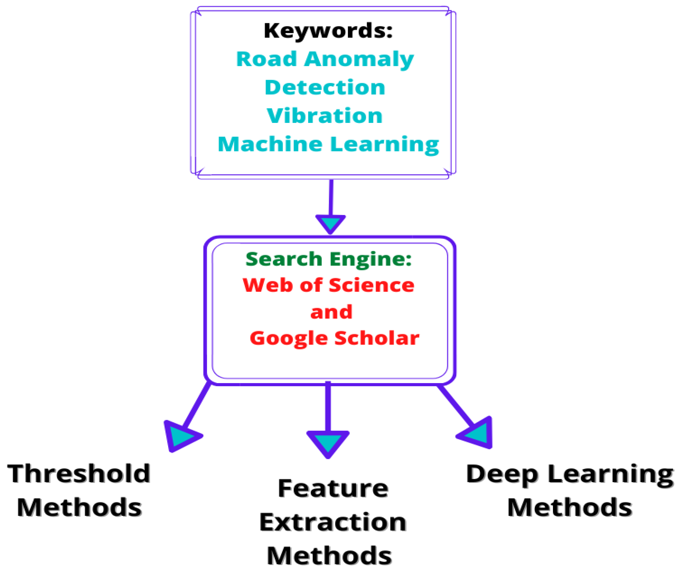
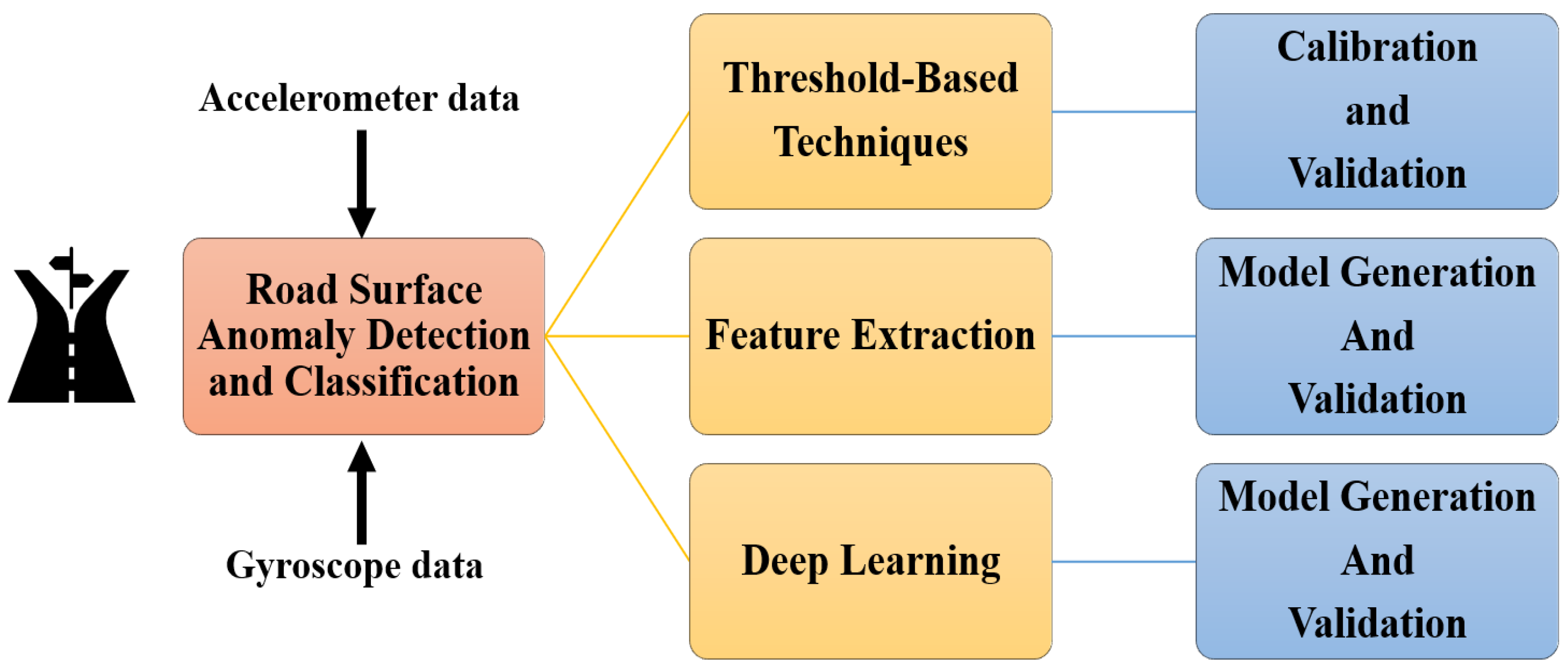
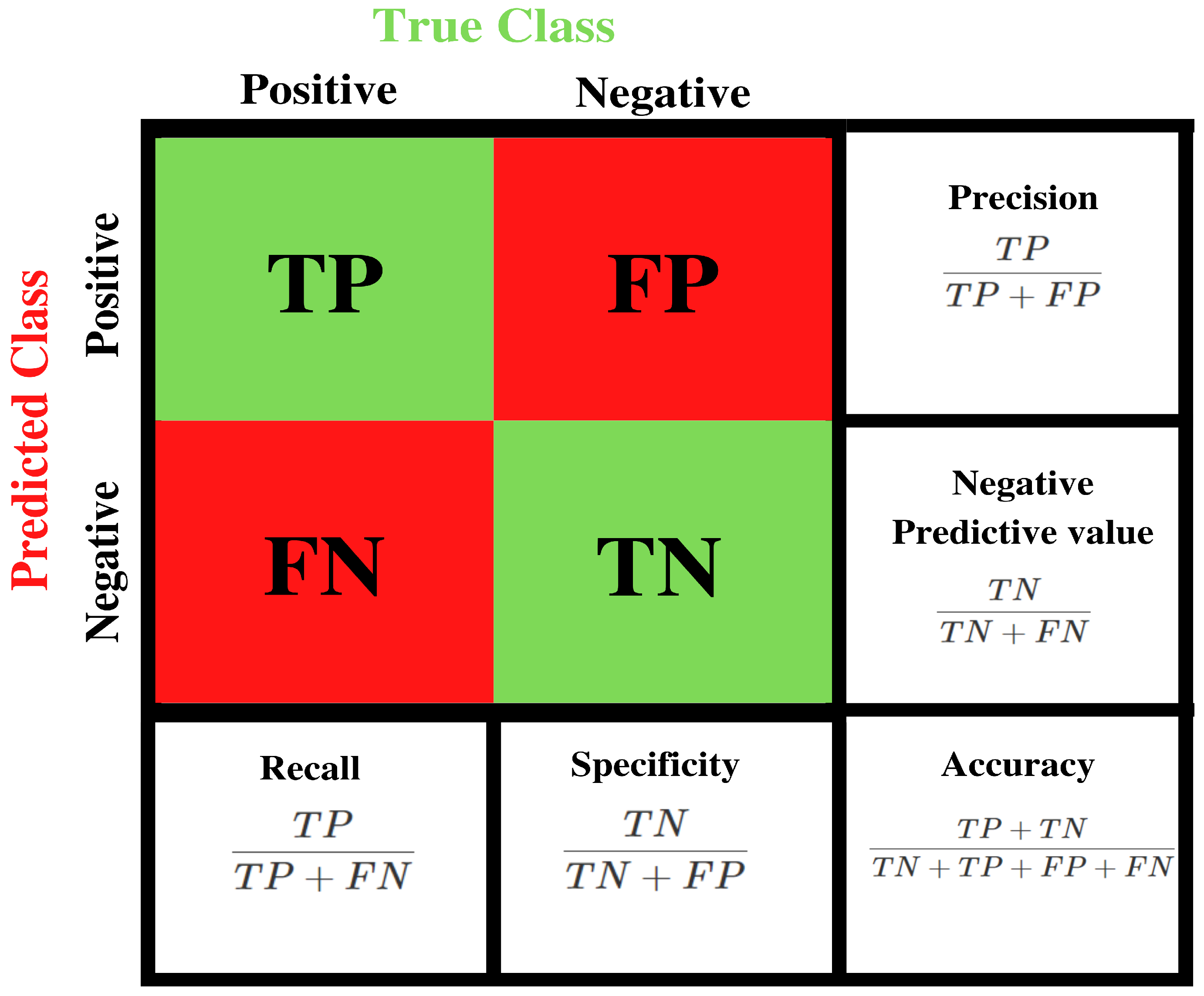
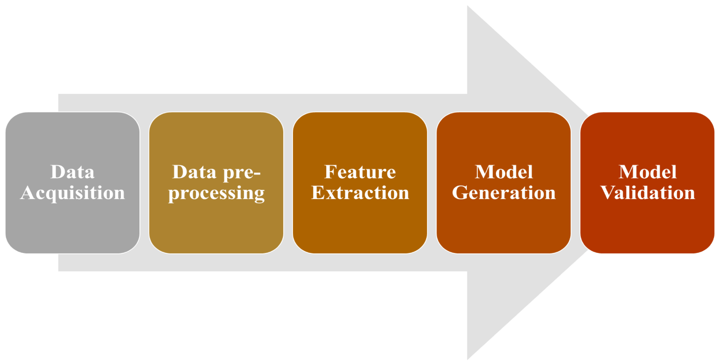
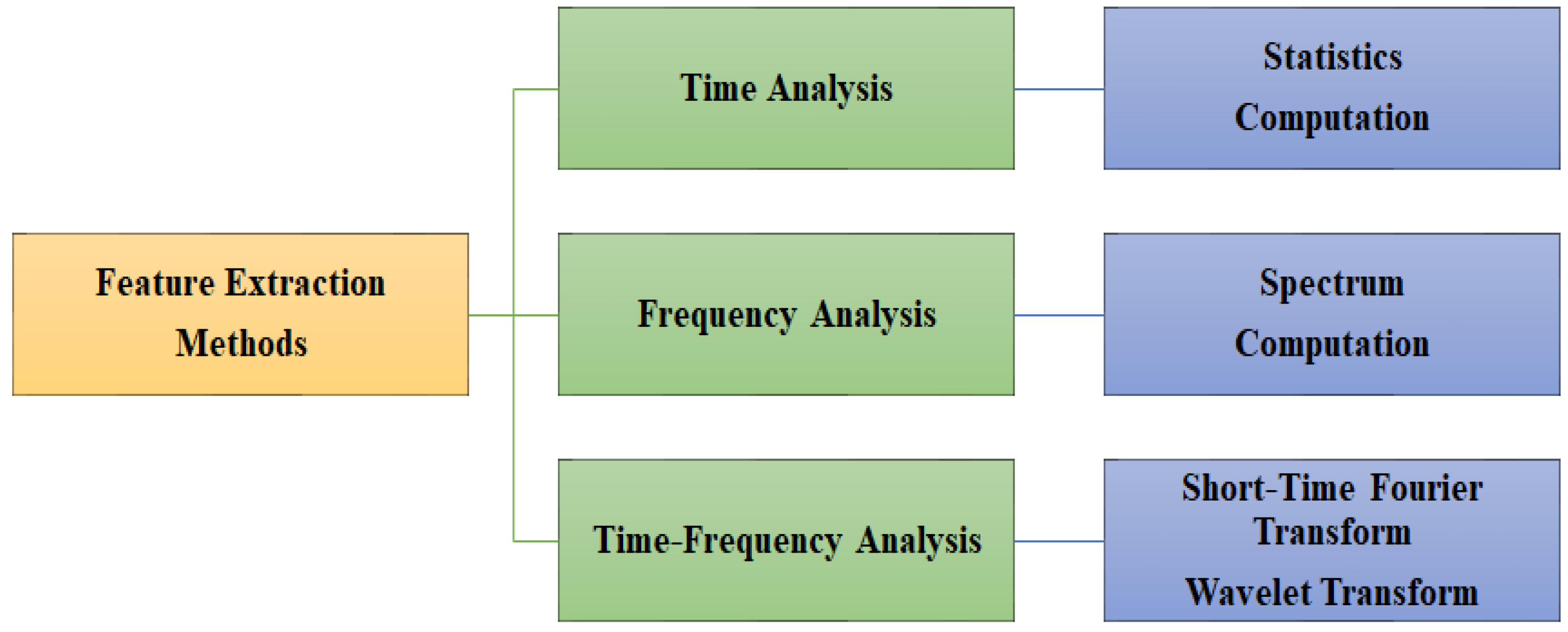
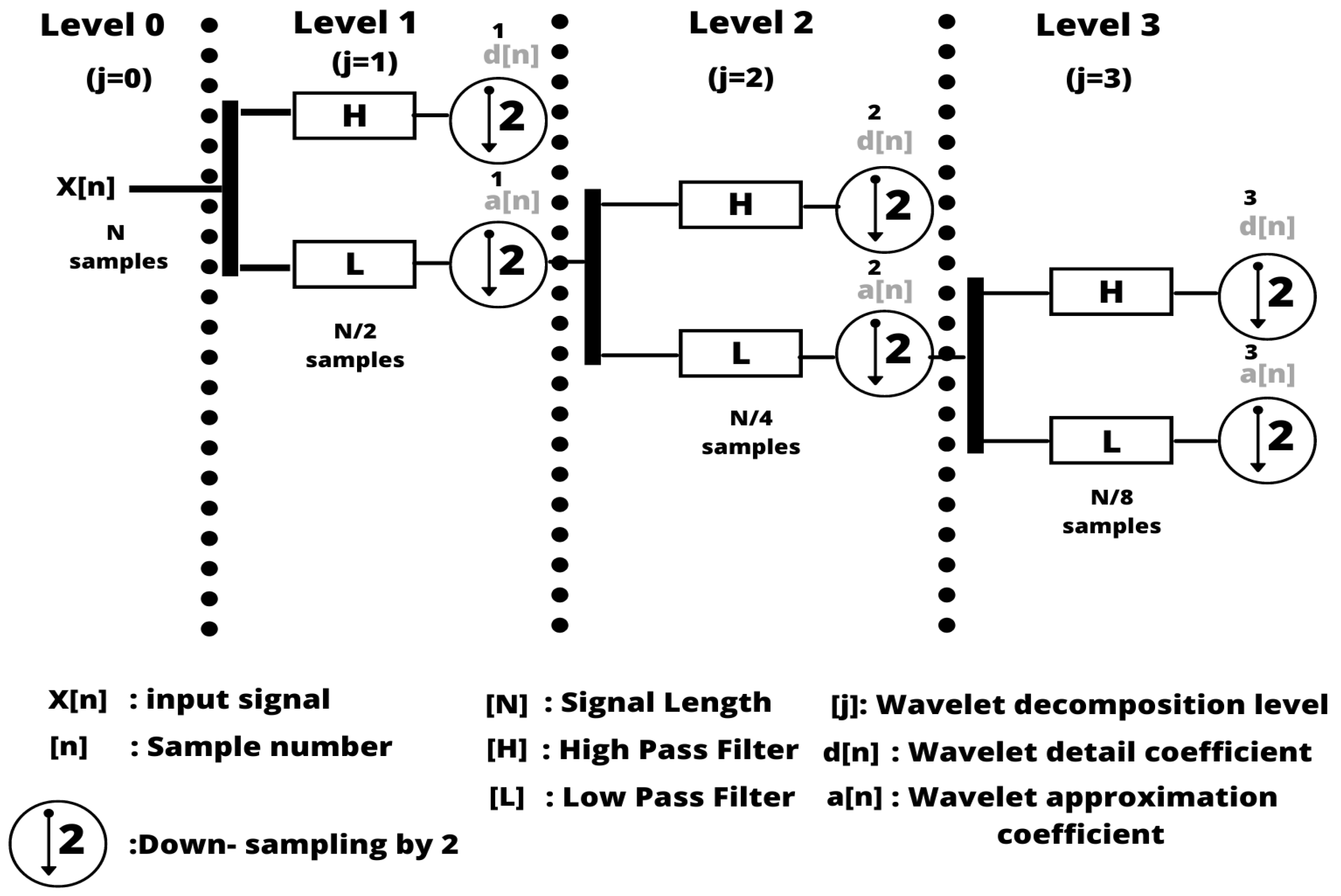
Table 1.
Advantages and disadvantages of road surface anomaly detection and classification techniques [11,16].
| Road Anomaly Detection Method | Advantages | Disadvantages |
|---|---|---|
| Vision-based | • Can be useful to determine the dimension of the anomaly. • Can be useful to determine the number of anomalies. • It is less expensive compared to 3D reconstruction. | • It is affected by light and shadows. • It cannot determine precisely the depth and shape of the anomaly compared to 3D reconstruction. |
| Vibration-based | • It is the most cost-effective method compared to vision and 3D reconstruction methods. • Real-time execution can be performed. | • It can be affected by the position and type of vehicle used. • It is complicated to determine the shape and depth of the anomaly. • It is necessary to pass over the anomaly. |
| 3D Reconstruction | • It can measure the shape and depth of the anomaly more precisely than the other techniques. | • Expensive method compared to vibration and vision techniques. |
Table 2.
Metrics used to evaluate the performance of threshold-based methods and machine learning models for the detection and classification of road surface anomalies [24,25].
| Metrics | Equation |
|---|---|
| Accuracy | |
| True Positive Rate/Recall/Sensitivity | |
| Specificity | |
| Precision | |
| False Positive Rate | |
| F1-Score | |
| TP: true positives, TN: true negatives, FP: false positives, FP: false negatives | |
Table 3.
Methods used for road anomaly detection and classification based on threshold techniques.
| Author | Year | Classified Road Anomalies | Algorithm | Reported Performance Metrics |
|---|---|---|---|---|
| Carlos et al. [14] | 2018 | Potholes Bumps Metal bumps | STDEV(Z) threshold | Average F1-score: 74.40% |
| Nguyen et al. [22] | 2019 | Potholes | Grubss Test and threshold (Z-THRESH) | Precision-Recall curves graphs. F1-score curves graphs. |
| Zheng et al. [21] | 2020 | Pothole Speed bump Metal bump | Query filter plus self-similarity | F1-score: greater than 70% for potholes, speed bumps, and metal bump. |
| Zheng et al. [23] | 2020 | Pothole Speed bump Metal bump | Threshold in combination with Random Forest and Dynamic Time Warping | F1-score: 93.90% for pothole F1-score: 87.4 % for speed bump F1-score: 81.9% for metal bump |
| Sattar et al. [11] | 2021 | Potholes Manholes Cracks Road joints | Hybrid approach Threshold plus Gaussian Mixture Model | Accuracy: 70% |
Table 4.
Methods used for road anomaly detection and classification based on feature extraction techniques.
Table 4.
Methods used for road anomaly detection and classification based on feature extraction techniques.
| Author | Year | Classified Road Anomalies | Algorithm | Performance Metrics |
|---|---|---|---|---|
| Celaya et al. [5] | 2018 | Speed bump | Logistic Regression | Accuracy: 97.14% |
| Annaisi et al. [36] | 2019 | Benign anomalies Defect of the road | One-class Support Vector Machine | Accuracy: 97.50% |
| Wu et al. [26] | 2020 | Potholes | Random Forest | Accuracy: 95.7% |
| Zhou et al. [37] | 2022 | Manholes | Support Vector Machine | Accuracy: 84.40% |
| Bustamante et al. [35] | 2022 | Pothole Speed bump Curve Plain | k-Nearest Neighbor | Accuracy: 95.55% |
| Ferjani et al. [18] | 2022 | Potholes Metal bumps Asphalt bumps Worn out roads | Decision Tree | Accuracy: 94.00% |
| Julio-Rodríguez et al. [38] | 2022 | Cobblestones Flatlands Transits | k-Nearest Neighbor | Accuracy: 93.20% |
Table 5.
Methods used for road anomaly detection and classification based on deep learning techniques.
Table 5.
Methods used for road anomaly detection and classification based on deep learning techniques.
| Author | Year | Classified Road Anomalies | Algorithm | Performance Metrics |
|---|---|---|---|---|
| Basavaraju et al. [42] | 2019 | Crack Pothole Smooth Road | Multilayer Perceptron | Accuracy: 92.12% |
| Varona et al. [1] | 2020 | Call Door Message Potholes Speed bump Street Gutter | Convolutional Neural Network | Accuracy: 93.00% |
| Baldini et al. [40] | 2020 | Potholes Cracks Transverse cracks Patches Rumble strips Speed bump | Convolutional Neural Network | Accuracy: 97.20% |
| Luo et al. [3] | 2020 | Pothole Bump Gravel Cobblestone Broken concrete | Recurrent Neural Network | Accuracy: 99.26% |
| Tiwari et al. [41] | 2020 | Good road Medium road Bad road | Convolutional Neural Network | Accuracy: 98.5% |
| Menegazzo et al. [43] | 2021 | Asphalt road Cobblestone road Dirt road | Convolutional Neural Network | Accuracy: 93.17% |
Table 6.
Summary of the type of signals used for road surface anomaly detection and classification through vibration-based techniques.
Table 6.
Summary of the type of signals used for road surface anomaly detection and classification through vibration-based techniques.
| Author | Year | Data Used for the Road Anomaly Detection and Classification |
|---|---|---|
| Carlos et al. [14] | 2018 | Z-axis of the accelerometer sensor. |
| Celaya et al. [5] | 2018 | X and Y axes gyroscope data. Y-axis accelerometer data. |
| Nguyen et al. [22] | 2019 | Z-axis of the accelerometer sensor. |
| Basavaraju et al. [42] | 2019 | Three-axes of the accelerometer data. |
| Anaissi et al. [36] | 2019 | Z-axis and X-axis of acceleration data. |
| Zheng et al. [21] | 2020 | Z-axis acceleration. |
| Luo et al. [3] | 2020 | Three-axes acceleration and gyroscope data. |
| Varona et al. [1] | 2020 | Three-axes accelerometer sensor. |
| Baldini et al. [40] | 2020 | Z-axis of the accelerometer sensor. Y-axis of the gyroscope sensor. |
| Wu et al. [26] | 2020 | Three-axes of the accelerometer sensor. |
| Baldini et al. [40] | 2020 | Three-axes acceleration and gyroscope data. |
| Sattar et al. [11] | 2021 | X, Y, and Z-axes linear acceleration (Calculated from gyroscope and magnetometer data) Gyroscope data used for reorientation of linear acceleration. |
| Menegazzo et al. [43] | 2021 | Three-axes acceleration and gyroscope data |
| Julio-Rodríguez et al. [38] | 2022 | Z and Y-axes linear acceleration Roll and pitch angles gyroscope data |
| Zhou et al. [37] | 2022 | Three-axes of accelerometer and gyroscope sensors. |
| Bustamante et al. [35] | 2022 | Three-axes accelerometer data. |
| Ferjani et al. [18] | 2022 | Three-axes accelerometer data. |
Table 7.
Time-domain features extracted from inertial sensors based on statistics for road surface anomaly detection and classification [5,18,37,56]. The n term refers to the length of the signal segment and is one single sample of the signal.
| Feature | Formula |
|---|---|
| Mean | |
| Variance | |
| Skewness | |
| Kurtosis | |
| Standard Deviation | |
| Max | |
| Min | |
| Range | |
| Mode | |
| Median | |
| Dynamic Range | |
| Root Mean-Square |
Table 8.
Time-frequency methods used to extract features from inertial sensors for the detection and classification of road surface anomalies.
Table 8.
Time-frequency methods used to extract features from inertial sensors for the detection and classification of road surface anomalies.
| Author | Method | Parameters |
|---|---|---|
| Baldini et al. [40] | STFT | Variation of window type. Variation of window length. Variation of overlapping between windows. |
| CWT | Morse wavelet used as mother wavelet Variation of frequency scales | |
| Li et al. [31] | CWT | Daubechies 3 wavelet (DB3) as the mother wavelet |
| Ferjani et al. [18] | DWT | Five level decomposition with a Daubechies 2 wavelet (DB2) |
| Wu et al. [26] | DWT | 3 levels Reverse Biorthogonal 3.1 wavelet |
| Basavaraju et al. [42] | DWT | Tested 3 wavelets at scales 4 and 5. Mortlet, Daubechies 6 and Daubechies 10 wavelets |
Table 9.
Advantages and disadvantages of road anomaly detection and classification systems through vibration-based techniques.
Table 9.
Advantages and disadvantages of road anomaly detection and classification systems through vibration-based techniques.
| Method | Advantages | Disadvantages |
|---|---|---|
| Threshold-based | • It does not require a training process. • Less computational costly compared to machine learning techniques. | • Threshold are set empirically. • It requires calibration of the thresholds. • It is susceptible to noise. |
| Feature Extraction | • Less computational costly compared to deep learning algorithms. • The models are less complex compared to deep learning solutions. | • It requires of a high quality dataset. • Its feature extraction process is not standardize. |
| Deep Learning | • Can achieve relatively high accuracy. • It does not require a feature extraction process. | • It requires a large sample size. • It lacks of interpretability. • It requires large training times. • It has a high computational cost. |
Publisher’s Note: MDPI stays neutral with regard to jurisdictional claims in published maps and institutional affiliations. |
© 2022 by the authors. Licensee MDPI, Basel, Switzerland. This article is an open access article distributed under the terms and conditions of the Creative Commons Attribution (CC BY) license (https://creativecommons.org/licenses/by/4.0/).
Share and Cite
MDPI and ACS Style
Martinez-Ríos, E.A.; Bustamante-Bello, M.R.; Arce-Sáenz, L.A. A Review of Road Surface Anomaly Detection and Classification Systems Based on Vibration-Based Techniques. Appl. Sci. 2022, 12, 9413. https://doi.org/10.3390/app12199413
AMA Style
Martinez-Ríos EA, Bustamante-Bello MR, Arce-Sáenz LA. A Review of Road Surface Anomaly Detection and Classification Systems Based on Vibration-Based Techniques. Applied Sciences. 2022; 12(19):9413. https://doi.org/10.3390/app12199413
Chicago/Turabian StyleMartinez-Ríos, Erick Axel, Martin Rogelio Bustamante-Bello, and Luis Alejandro Arce-Sáenz. 2022. "A Review of Road Surface Anomaly Detection and Classification Systems Based on Vibration-Based Techniques" Applied Sciences 12, no. 19: 9413. https://doi.org/10.3390/app12199413
Note that from the first issue of 2016, this journal uses article numbers instead of page numbers. See further details here.