Combining Biomechanical Features and Machine Learning Approaches to Identify Fencers’ Levels for Training Support

Abstract

Nowadays, modern technology is widespread in sports; therefore, finding an excellent approach to extracting knowledge from data is necessary. Machine Learning (ML) algorithms can be beneficial in biomechanical data management because they can handle a large amount of data. A fencing lunge represents an exciting scenario since it necessitates neuromuscular coordination, strength, and proper execution to succeed in a competition. However, to investigate and analyze a sports movement, it is necessary to understand its nature and goal and to identify the factors that affect its performance. The present work aims to define the best model to screen élite and novice fencers to develop further a tool to support athletes’ and trainers’ activity. We conducted a cross-sectional study in a fencing club to collect anthropometric and biomechanical data from élite and novice fencers. Wearable sensors were used to collect biomechanical data, including a wireless inertial system and four surface electromyographic (sEMG) probes. Four different ML algorithms were trained for each dataset, and the most accurate was further trained with hyperparameter tuning. The best Machine Learning algorithm was Multilayer Perceptron (MLP), which had $96.0$% accuracy and 90% precision, recall, and F1-score when predicting class novice (0); and 93% precision, recall, and F1-score when predicting class élite (1). Interestingly, the MLP model has a slightly higher capacity to recognize élite fencers than novices; this is important to determine which training planning and execution are the best to achieve good performances.

1. Introduction

Fencing, one of the oldest sports, places many demands on the body regarding neuromuscular coordination, strength, power, and musculoskeletal system impact. Fencers align the leading foot with the opponent’s stance in the basic en guard gesture and place the back foot at ${90}^{\circ }$ to the leading foot to maintain stability [1]. Furthermore, a fencer’s effectiveness is highly dependent on the quickness of his/her motions in response to the opponent’s action and his/her ability to anticipate the opponent using visual, kinaesthetic (dodge and parry), and acoustic stimuli [2]. The lunge movement starts with upper body movement, combined with the lower legs through the kinetic chain at the ankle, knee, and hip joints, to move the sword as quickly as possible towards the opponent to achieve a touch [3]. All of the rapid "propulsion" and "dodge" movements of attack/defense further expose fencers to impacts, explosive forces, power absorption, and shear forces of various magnitudes, distributed asymmetrically across the body [1]. Resulting of these dynamic and repetitive movements in fencing matches, fencing injuries are quite prevalent among athletes.

The use of technology in sports is rapidly increasing, and biomechanical analysis in most sports is routine at the élite level these days. Sports biomechanics allows detailed analysis of sports movements to improve sports performance and/or lessen injury risk. One of the significant aims of sports data analysis is to assist in training. Motion capture is one of the most frequently used techniques in sports analysis; however, recent technological developments have produced inexpensive, non-invasive, wearable sensors that are ideal for obtaining sports performance measures during training or competition. The usefulness of wearable sensors for sports analysis has been shown in several papers [4,5]: they are a reliable tool, able to benefit athletes of all levels, especially when complemented within a sensor fusion network and provide a large amount of high accuracy biomechanical data. However, with the large amount of data produced, finding a method to identify a meaningful relationship between data and extract the relevant information became necessary. In healthcare, user monitoring can be carried out in different ways by ensuring different levels of awareness [6,7,8] and security [9,10,11] for diagnostic and/or therapeutic purposes [12,13,14,15,16,17,18,19,20].

In the same way, predictive modeling methodologies could be applied to prove the efficiency and effectiveness of various fencing assault strategies. It is essential to understand which data should be saved and how to use it best. Sports establishments have an advantage over other teams by finding an acceptable way to extract the meaning from the available data and turn it into practical knowledge [21]. Combining wearable sensors and ML algorithms could enhance training by providing tools for analyzing actions. Recent studies have shown that élite fencers exhibited sequential coordination of upper and lower limb movements with coherent muscle activation patterns, compared to novice fencers [1]. Thus, élite fencers can fine-tune the techniques of fencers qualitatively, and trainers can use them to identify areas where trainees can improve. The present study aimed to combine biomechanical data related to the lunge gesture and different machine learning approaches to find the best model to classify the levels of performance of fencers, élite or novice. This gave us a useful tool to improve athletes’ performance and trainers’ activity. The paper is organized as follows. Section 2 provides an overview of related work and technologies investigated as background knowledge, including fundamental notions of fencing and lunge movement determinants. Section 3 describes the collected biomechanical data and the Machine Learning methods that were trained to predict the fencers’ categories (élite or novice). Section 4 outlines the experimental setting and assesses event-log data with state-of-the-art evaluation metrics. Finally, Section 5 presents the concluding remarks.

2. Background and Related Works

In this section, we review the state-of-the-art biomechanical aspects of the lunge to identify the most critical aspects from kinematic and muscular perspectives. In addition, a few studies were identified in the literature which used Machine Learning algorithms as training support in fencing.

2.1. Background

Understanding the biomechanics and demands of a sport provides a pathway to injury prevention and safety promotion [22,23,24]. An analysis of the biomechanics of a sport can also improve athletes’ skills, tactics, and overall performance and competitiveness. Biomechanical analysis can be applied in sports, allowing not only an improvement of sports performance but also the prevention of injuries and recovery from them [5]. In this study, we analyzed the biomechanics of the lunge in fencing.

The lunge is the most frequently used form of attack in fencing and is performed extensively during competition. The starting position of this motor gesture is the en garde position, which can influence the speed and distance traveled, the two main lunge influential factors. Therefore, we analyze in Section 2.1.1 the en garde position; in Section 2.1.2 the lunge distance traveled; in Section 2.1.3 the lunge speed; and lastly, in Section 2.1.4, the biomechanical aspects of the lunge.

2.1.1. En Garde Position

The starting position of the fencing lunge is the en garde position, in which the fencer aligns the front foot against the opponent, and the back foot is placed at ${90}^{\circ }$ to the front foot to ensure stability [1]. Therefore, both feet are initially in contact with the ground, and no ground reaction force (GRF) is acting after removing the body weight. The lunge begins when the front foot loses contact with the ground, and the back foot pushes the fencer’s center of gravity (CG) forward, exerting a force against the ground.

From the en garde position, the front leg muscles are activated first than the back leg ones [25]. This position allows the fencer to shift from attack to defense quickly, and vice versa, by varying the support base and CG. This ability is crucial because a fencer must be able to quickly switch from a current or expected action to a new one that can fit an opponent’s feint (or even attack). Although perceptual and psychomotor skills mainly determine this, a fencer must have the physical requirements to capitalize on this. Given the rebound, the demand for the semi-squat position and the quick response, it would be helpful to suggest exercises that train the development of strength and plyometric ability [26].

2.1.2. Distance Traveled

A lunge enables the fencer to cover extremely long distances, which differ from fencer to fencer. Many studies choose to standardize the distance each fencer must travel to conduct a study without identifying the distance traveled as a variable. To achieve a fully extended lunge, the horizontal distance between the tip of the sword in the en garde posture and the target was standardized by multiplying each fencer’s standing height by $1.5$ [25].

2.1.3. Speed

The lunge speed can be described as the sword speed, the peak of the horizontal component of CG speed (HPV), or the body’s average horizontal CG speed [25]. The last one may not be an appropriate variable for comparison. Therefore, HPV was supposed to be the most accurate variable to represent lunge speed. It was demonstrated that élite fencers could perform a lunge with a higher HPV than novice fencers. Previous research suggested that HPV and back-leg extensor strength and power are closely correlated. In addition, élite fencers’ peak ground reaction force (PGRF) was substantially higher than that of novice fencers; both kinetic and kinematic parameters of the lower limb joints significantly differed between the two groups [25]. To achieve touché, the lunge action begins from the armed arm, followed by legs through a kinetic chain involving the ankle, knee, and hip joints. Due to the increased speed of the center of mass (CM) generated from the foot-to-ground interaction, élite fencers perform the touché with a faster sword movement than novices [3]. Finding the precise movement factors contributing to a high sword velocity could offer some insights into ideal movement tactics. It is evident that increasing the lower limbs’ capacity to move faster and with greater force should speed up the lunge and, by extension, the touché. However, it is unclear how much any potential variations in the lower extremities’ movement strategies would affect the execution of a better lunge [3]. The back extreme knee range of motion, peak hip flexion in the sagittal plane, and hip flexion should be more extensive at the end of the lunge in élite fencers than in novice fencers, critical determinants of sword speed. The strongest indicator of force measurement in the lunge is concentric peak force [3]. To ensure the best performance during a competition, fencers should lower themselves into a low en garde position to increase knee flexion (quadriceps and technocratic muscles must be strong) and pelvic flexion (Iliopsoas and Rectus Femoris muscles must be strengthened). Finally, élite fencers extend their armed arms with the foil faster than novices. The foil’s velocity is increased due to the increased postural support velocity [3].

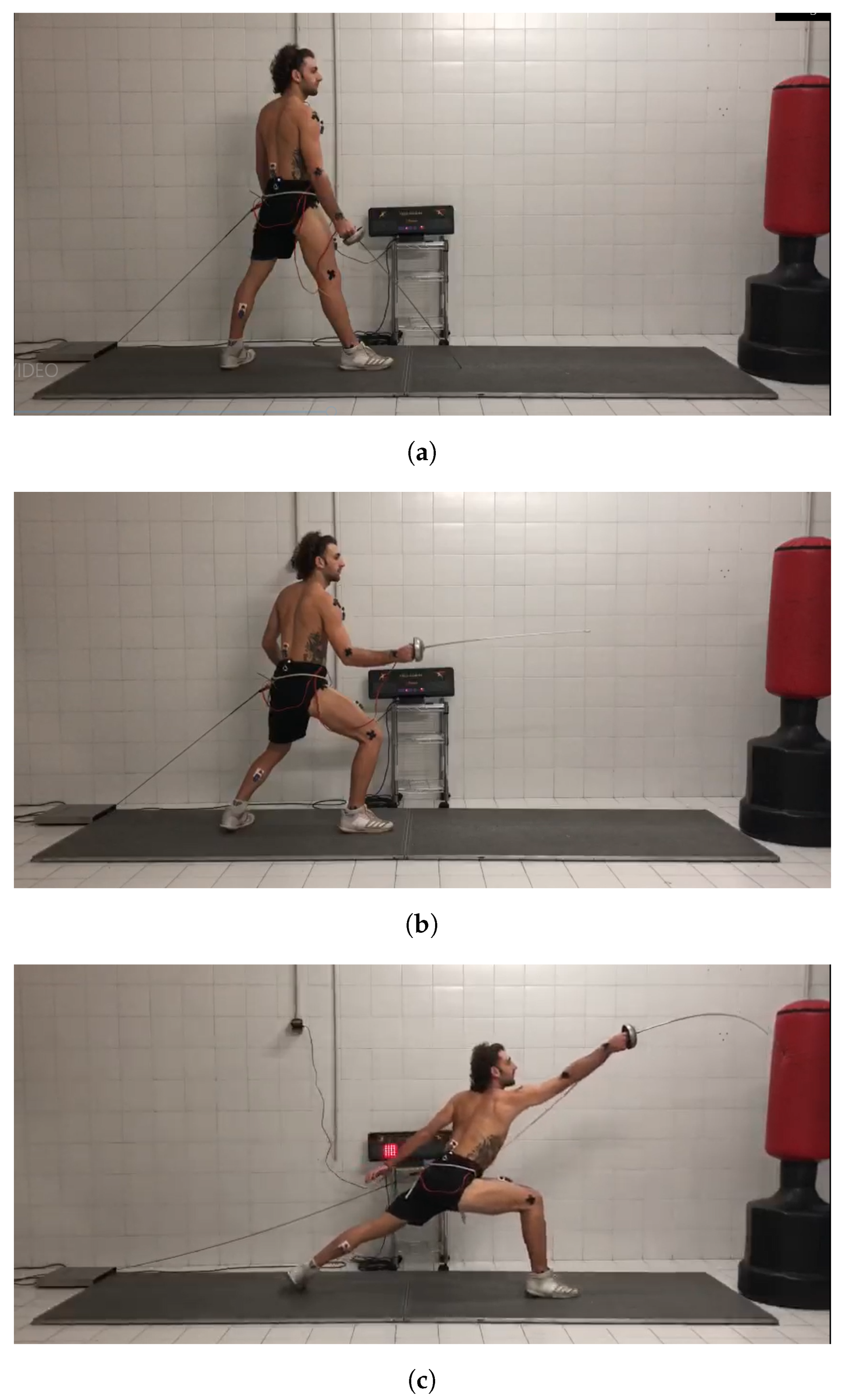
2.1.4. Lunge

The fencer begins to exert force with the rear foot in response to a stimulus, generally the opponent’s action and accelerates forward in a timing sequence that usually begins with a push of the armed arm and a stride forward with the front foot. This is the acceleration phase, which finishes when the back foot comes to a halt and pushes against the floor, followed by the flight phase, which ends when the front foot makes contact with the ground. Finally, when the target is achieved, the force applied by the front foot acts as a brake, slowing down the horizontal speed. During the acceleration phase, the fencer modifies his action according to the opponent’s unpredictable action [26,27,28]. The leading leg’s peak force-time (TPF) and its length and flexibility were the best predictors of lunge performance. Using the correct model, the fencer’s level can be determined by highlighting and detecting certain factors, such as distance traveled, speed reached, and muscle and joint activity. Regarding élite and novice, the first group covered a longer lunge distance, and the hand preceded the foot for both the élite and the novice. Many studies have also addressed the variations in response time, muscle activation pattern, and joint kinematics in response to various visual, acoustic, or tactile stimuli [2,29,30,31,32,33].

In particular, Sorel and colleagues [2] proposed an innovative fencing lunge simulator for fencers’ training under different conditions, i.e., fixed (target stationery), moving (target in motion), and uncertain (target stationery on in motion) conditions. The population in this study was composed of fencers with different competition levels. The findings showed that the accuracy and success of the lunging decreased when comparing the performance under fixed conditions to moving and uncertain ones.

Gutierrez-Davila and colleagues considered the flight time, the horizontal velocity at the end of the acceleration phase, and the length of the lunge as factors that could differentiate between two groups of athletes (élite and novice fencers). The athlete had to perform the lunge movement after viewing a stimulus projected on a screen. The factors mentioned before were higher for the élite group, along with other variables related to the temporal sequence of movement. Additionally, the coordination of fencing movements constitutes a factor that differentiates élite fencers from novice ones [30]. The same group studied the temporal parameters of the reaction response, the execution speed, and the precision and coordination of the movement pattern to analyze the influence that changing targets during a simple long lunge attack exerts.The findings showed that compared to an attack carried out with a straight thrust, the response time, movement time, and the time used in the acceleration phase of the CM significantly increased when the target changed. After the acceleration phase, the center of mass speed and horizontal distance significantly decreased while the errors increased. However, there were no appreciable changes in the temporal sequence of the movement pattern [31].

With this evidence, recently, Chen and colleagues concluded that intrinsic and athlete-specific factors (sex-specific differences, anthropometry, muscle strength and asymmetry), extrinsic factors (weapon, footwear, fencing piste, training, and conditioning), and basic biomechanics (i.e., posture, kinematics, joint coordination, synergy, muscle coordination, and synergy) were factors that influence and determine variances in lunge execution based on various research [1].

2.2. Related Works

The usage of Machine Learning and its practical applications are of interest to sports scientists because they have significant consequences for their industry. In fact, it has already influenced:

• The devices used to collect data;
• The knowledge obtained from device-gathered data (3D kinematic and vertical ground reaction forces may be predicted);
• The processing of data from devices (classification methods can separate data into relevant packages that would have previously required sports scientists to spend much time on them);
• How processed data can improve our comprehension of athletic performance and injury risk prediction.

The objectivity of decision-making in sports science is projected to improve significantly by using Machine Learning during the coming ten years. According to studies, Machine Learning can predict future injuries based on pre-season measurements, identify movement strategies within a cohort, allow the identification of movement-specific injury risk factors, and recognize healthy people who exhibit movement patterns that are similar to those of injured people [34].

Malawski and colleagues [35] trained a Support Vector Machine (SVM) to test whether it would be preferable to use an inertial measurement unit (IMU) or a Kinect to record and classify fencing footwork to aid in fencer and coach training. The detection with the Kinect proved to be highly effective; it simultaneously achieved $100\%$ recall and $100\%$ precision. The inertial-based technique had the best detection performance, with $99.38\%$ recall and $98.77\%$ precision. The proposed approach has proven to be effective at providing pertinent feedback. However, it would be advantageous to further increase accuracy, particularly for the hand-time parameter, to enable even the most experienced fencers to improve this movement. Kinect’s algorithm was also built for frontal postures, whereas fencing footwork is seen from the side. As a result, more precise tracking might be accomplished with a method designed specifically for fencing activities with a greater sample rate. It is important to note that the sensor’s proper body location must be identified for IMU to compete with Kinect [35].

In this regard, O’Reilly and colleagues [36] used five IMUs placed on the lumbar spine, thighs, and shanks to categorize proper and improper lunge techniques and precise lunge technique variations. The IMU data’s time and frequency domain features were used to train and evaluate SVM, k-nearest neighbors, Naïve Bayes, and random forest. Only the random forest was selected due to its superior classification performance and its classification performance effectiveness. They used the permutation feature importance method of the random forest to analyze the most crucial attributes. One IMU on the right thigh can have $78\%$ sensitivity and $83\%$ specificity with a full feature dataset. The left shank had the lowest sensitivity and specificity for binary classification when employing a single IMU, at $40\%$ and $82\%$, respectively. Regarding multi-class classification and binary classification (which has an accuracy of $90\%$), the five-IMU setup performed best ($70\%$ accuracy). A smaller IMU set with three IMUs placed on the lumbar region and both shanks also yielded accurate classification results. Categorizing quality is comparable to utilizing all features, even just $20\%$ of the top-ranked characteristics [36].

Malawski and colleagues [37] classified fundamental footwork movements (step forward, step backward, rapid lunge, lunge with increased speed, lunge with waiting, and jumping-sliding lunge) in a cohort of 10 fencers with varying levels of experience using data from just one IMU placed on the knee. A spline interpolation was used in the pre-processing stage to ensure that each sample was the same length, following the division of each signal into segments of equal size and $50\%$ overlap. The three types of features they considered for each window—time-domain features, frequency-domain features, and Wavelet features—led to the conclusion that time-domain features offered the most effective recognition. Additionally, they solely used accelerometer data because the gyroscope data comparison did not show a significant improvement. They compared Dynamic Time Warping (DTW), DTW-feat, SVM, and RBF-SVM for classification purposes. The trials were performed utilizing a 5-fold cross-validation for each performance individually (PD) and leave-one-out for the entire dataset (PI). They discovered that SVMs constructed using the suggested dataset have more significant generalization potential than DTW. As a result, SVM can compete with DTW regarding processing speed and accuracy [37].

With this evidence, it emerged that besides the great interest in using modern enabling technologies in sports, only a few have preliminary attempted to apply them to fencing. We propose a combination of wearable sensors and ML algorithms to classify the fencer’s category into élite or novice, thereby allowing feedback to the fencer and coach and an improved training strategy.

3. Materials and Methods

Thanks to newly available technologies, biomechanical data acquisition in sports can be done using optical or non-optical systems. Optical systems include optoelectronic systems (MoCap), which can be marker-based or markerless, such as the Kinect (RGB camera and depth sensor). Non-optical systems include inertial systems. The following considerations guided the choice of experimental settings reported in this paper. Firstly, effective motion tracking using an RGB camera is highly difficult due to quick motions, the presence of several people, and challenging lighting conditions in training rooms. However, deep learning techniques accurately identified persons in RGB movies. Secondly, MoCaps are computationally too expensive to offer the necessary precision for real-time sports. They demand the use of numerous synchronized cameras and the wearing of many markers, making them expensive and impracticable for use in sporting events. Furthermore, to avoid occlusions, the area between the sensor and the tracked person must remain empty, which is a substantial restriction in training facilities. The athlete also needs to stay within the depth camera’s field of vision. Finally, monitoring joint rotation with depth sensors is challenging, which is crucial in sports [35]. On the other hand, IMUs, even though they must be placed on the athlete, they do not need a well-organized workspace to be used [4]. IMUs can measure acceleration and angular velocity, but because errors can accumulate during the integration of the acceleration data, they are far less helpful for monitoring position and velocity. For these reasons, magnetometer information is integrated using a sensor fusion technique, usually a Kalman filter. Moreover, IMUs have a greater sampling frequency, often between 50 and 400 Hz, as opposed to a typical depth sensor’s 30 Hz. When compared to the visual data from the Kinect (RGB camera), the information provided by IMUs regarding acceleration, angular velocity, and the magnetic field is very different. Nevertheless, previous studies have found that both modalities help support real-time sports training. Therefore, when selecting the sensor for sports motion analysis, ease of use may be a deciding factor. It is worth noting that tracking direction with an IMU may be essential for assessing sports actions that involve rotation, such as fencing during the lunge [35].

This section introduces the (i) study population, (ii) study design, and (iii) algorithm used for preprocessing and classification purposes. Specifically, Section 3.2 depicts the study population and inclusion criteria; Section 3.3 depicts the instrumentation used during data collection; Section 3.4 depicts the acquisition protocol; and Section 3.5 depicts the biomechanical data preprocessing to identify the data associated with lunge movement. Section 3.6 depicts the principal component analysis algorithm used for dimensionality reduction; Section 3.7 depicts the Machine Learning algorithm selected and used in this study and how Machine Learning algorithms were trained and tested. The data follow the logical flow represented in Figure 1.

3.1. Experiment Environments

The algorithms implementation code was written entirely within the Pycharm application utilizing the Python 3.9.0 programming tool with an Intel $i7$ processor, CPU $11800H@2.30$ GHz, 1 TB SSD, 16 GB Random Access Memory (RAM), and Windows 11 operating system computing environment.

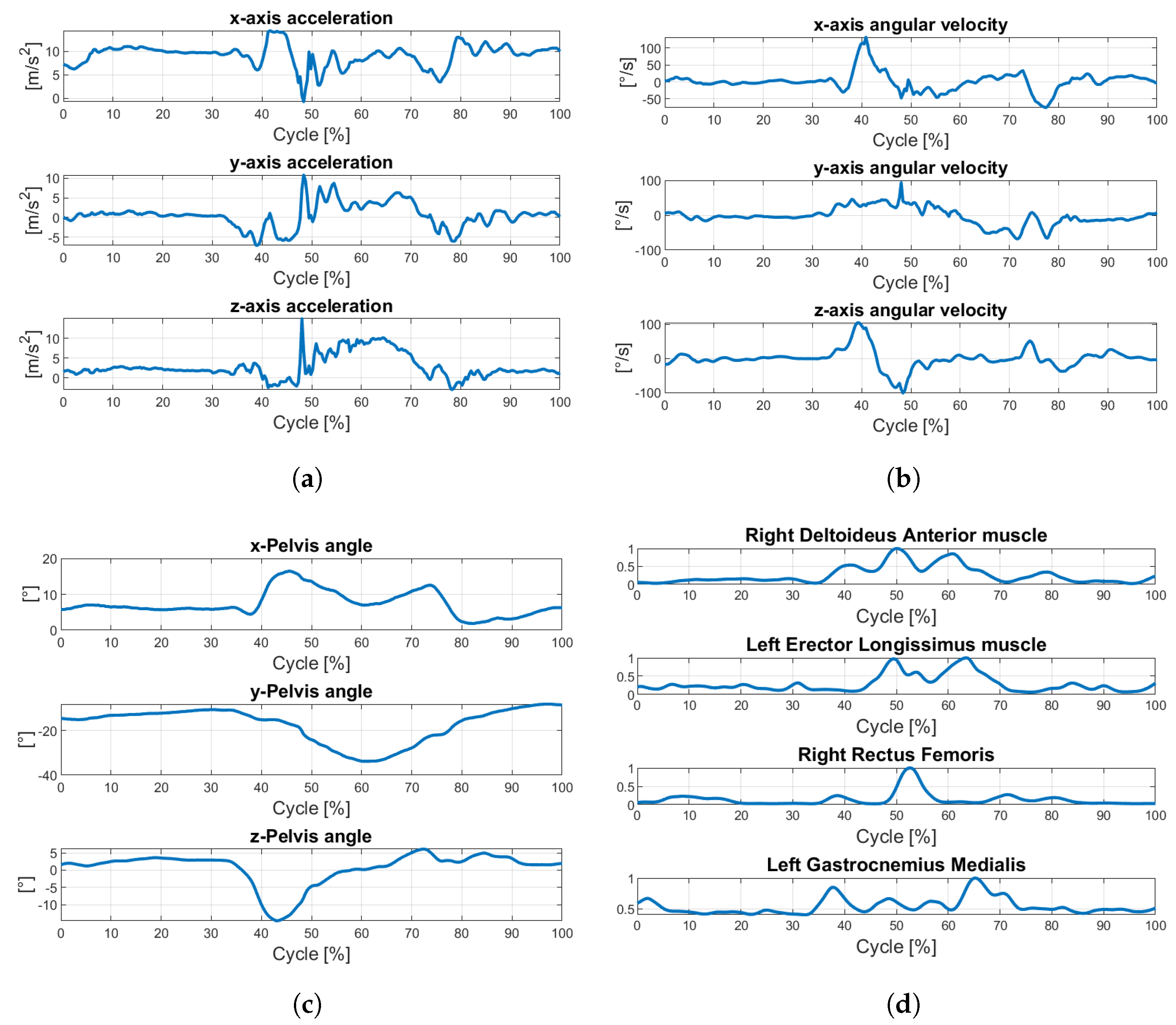
3.2. Data Collection

Twenty-one male and female fencers (17 male and 4 female fencers) participated in this cross-sectional study, all belonging to the A.s.d. CLUB SCHERMA BARI team. Eight of them were classified as novice fencers, and the other thirteen fencers were élite fencers. They practiced epée and foil. Their ages ranged from 8 to 35 years old. In the last six months before the test, they were free from lower-extremity musculoskeletal injuries. Subjects unable to understand the required actions were excluded from the study. The study, with its measurements and data collections, followed the Helsinki Declaration of 1975. All participants provided written informed consent for the study before their trial.

Data collected from the athletes during the study, using the devices described in Section 3.3, represented the dataset for the ML algorithms, which consisted of samples on the rows and features on the columns. Each subject performed all the different tasks at least two times, for a total of 6 trials per subject placed in rows within our dataset. There were 13 features used to train the different Machine Learning algorithms: tri-axial accelerations, tri-axial angular velocities, tri-axial pelvis angles, and four muscle envelopes. Each of these features is a two-dimensional signal over time, each being represented by 500 records. Each column of the dataset is a one-record of the individual feature. Therefore, our dataset had 126 rows and 6500 columns.

3.3. Instruments

A professional fencing competition field was recreated, with a platform consisting of two parts with a total length of $1.80$ m and a set goal at the end. On one side of the platform, we placed a scorer to allow the fencer to confirm that the touch had been made. Kinematic data were collected using the inertial motion system BTS G-SENSOR 2 (BTS Bioengineering S.p.A., Italy) with a sampling frequency of 100 Hz. This wearable and wireless device is composed of a tri-axial accelerometer with levels of sensitivity ($\pm 2$, $\pm 4$, $\pm 8$, $\pm 16$ g), a tri-axial gyroscope (16 bit/axes) with multiple levels of sensitivity ($\pm 250$, $\pm 500$, $\pm 1000$, $\pm 2000$${}^{\circ }$/s), and a magnetometer (13 bit/axes) with a dynamic range of $\pm 1200$ μT, all of which are linked using advanced sensor fusion technology. The IMU was attached to the back of the athlete with an elastic bend (at the level of the L5 or S1 vertebra), sending data to a PC over a Bluetooth interface.

The sEMG signal was collected with four wearable probes, BTS FREEEMG 1000 (BTS Bioengineering S.p.A., Garbagnate Milanese, Italy). The surface electromyographic signal was sampled at a rate of 1000 Hz by a 16-bit analog-to-digital converter. These probes were applied to the muscles of interest following SENIAM recommendations with adhesive Ag/AgCl electrodes. The target muscles were deltoideus anterior (DLTA) and rectus femoris (RF), both on the armed side; erector longissimus muscle (LONG) and gastrocnemius medialis (GAM) on the opposite side. An adhesive patch was used to better stop the EMG probes on the target muscles because of the abrupt action. Both wearable devices are small in size and lightweight so as not to impair the subject when performing motor gestures.

All the devices were synchronized by the acquisition software BTS EMG-Analyzer, in which the designed protocol was defined. Lastly, for video acquisition, an iPhone camera was mounted on a tripod in front of the platform, allowing for capture along the sagittal plane of the subject at a distance of $3.80$ m from the platform and a height of $1.14$ m above the ground.

3.4. Experimental Protocol

Stretching and a five-minute free-body warm-up were conducted by each participant. Each participant was familiarized with the testing area and conditions after warming up. Before starting with the fence test, biographical information (name, surname, age) was collected. In addition, some anthropometric information was acquired: weight (W), height in a standing position (H), height in en garde position (HGUARD), length of the front leg in the en garde position (LLL), the circumference of the front thigh (CLL), and circumference of the armed arm (CUL). Finally, their respective membership categories, specialties practiced, and weapon length (Leq) were requested.

Table 1. Sociodemographic and anthropometric variables according to category (novice and élite). (All data are shown as mean ± (standard deviation) for continuous variables).

Variables	Novice	élite	Effect Size (ES)
Age (years)	10.50 ± 3.14	$16.31\pm 5.85$	0.72 (0.48, 0.97)
BMI (kg/m${}^2$)	$18.87\pm 3.87$	$22.29\pm 3.82$	0.39 (0.09, 0.73)
W (kg)	$39.30\pm 11.87$	$61.95\pm 11.86$	0.68 (0.48, 0.9)
H (m)	$1.43\pm 0.08$	$1.66\pm 0.12$	0.75 (0.63, 0.9)
HGUARD (m)	$1.32\pm 0.08$	$1.56\pm 0.13$	0.76 (0.63, 0.91)
LLL (cm)	$73.66\pm 7.3$	$90.00\pm 8.36$	0.74 (0.61, 0.9)
CLL (cm)	$40.70\pm 6.38$	$50.28\pm 9.58$	0.53 (0.26, 0.83)
CUL (cm)	$22.70\pm 5.55$	$27.46\pm 7.67$	0.44 (0.12, 0.77)
Leq (cm)	$79.5\pm 2.67$	$88.75\pm 2.23$	0.86 (0.77, 0.95)

shows the sociodemographic and anthropometric variables for the whole sample according to the fencers’ membership categories. To detect significant practical differences in the magnitude of association, we estimated effect size (ES) and categorized it into small (equal or less than $0.2$), medium (equal or less than $0.5$), or large (equal or greater than $0.8$) according to Cohen’s criteria. Wilcoxon’s effect size has been performed for continuous variables. Data analyses were performed using RStudio software, version 1.2.5042. All the variables showed medium to large significant differences between the fencers’ categories.

Afterward, the subject’s skin was prepared to place the four sEMG probes on it. In the first part of the acquisition, the subject was asked to perform four different motor tasks to acquire each muscle’s Maximum Voluntary Contraction (MVC). Each test was performed for 30 s with an intermediate pause of 5 s, repeated three times. The inertial system was then attached to the fencer, who was given detailed instructions on completing each assignment. The fencing test was performed, which consisted of performing three fundamental fencing exercises:

• Explosive lunge: the subject had to execute a lunge that was not demonstrative but pushed in order to hit the target as fast as possible;
• Step forward lunge: the subject was placed further away from the lunge, as the exercise consists of carrying out an offensive action in which the fencer must take a step forward to get to lunge distance in order to execute it and then stop the target;
• Step back lunge: the subject takes a step backward to get within lunge distance and then scores a hit.

The lunging cycle was divided as follows: At the beginning of each task, the subject was placed in a relaxed static position. After the trainer’s command, he switched to the en garde position. At another command from the trainer, he sank and then finished by returning to guard. The lunging movement cycle can be observed in Figure 2. In particular, Figure 2a shows the start position. In Figure 2b, the en garde position is shown, and lastly, in Figure 2c is the final lunge. Each task was acquired 2 times, and each fencer chose the distance from the target through a series of tests.

3.5. Data Pre-Processing

Collected data were imported to MATLAB R2020a (https://it.mathworks.com/products/new_products/release2020a.html, accessed on 18 March 2020). The inertial system provided in output its orientation in time in the form of Euler angles referred to as the reference system of the sensor itself. These data made it possible to calculate the pelvis joint kinematics, also expressed as Euler angles, referred to as the pelvis reference system. The latter is obtained by making an anticlockwise rotation of the sensor reference system’s ${180}^{\circ }$. EMG signals were processed with the following protocol: Butterworth bandpass filter with cut-off frequencies of 10 and 450 Hz and Butterworth low-pass filter with a cut-off frequency of 6 Hz. A threshold algorithm was applied to detect each lunge task’s start and end. First, the Euclidean acceleration norm (Equation (1)) was calculated as follows:

$$\begin{array}{c}\hfill ACC=\sqrt{AC{C}_x^2+AC{C}_y^2+AC{C}_z^2}\end{array}$$

(1)

where $AC{C}_x$, $AC{C}_y$, and $AC{C}_z$ are, respectively, the acceleration components expressed in the sensor reference system along the x, y, and z axes. The subject was at rest in the first 3 s of acquisition due to the necessary sensor stabilization phase. Therefore, this time window (Equation (2)) was used to calculate the mean value and the standard deviation to obtain the threshold T value as follows:

$$\begin{array}{c}\hfill T=\mu +J\times \sigma \end{array}$$

(2)

where $\mu$ and $\sigma$ are the mean and standard deviation of the acceleration norm during a period of inactivity (time window), and J represents a numerical constant that takes on varying values depending on the case. In this study, $J=3$. The signal was considered a “lunge movement” if its over-threshold duration was greater than 70 ms. The end of the lunge coincided with the index of the last over—threshold sample, $0.2$ s before the first activation was considered as the beginning of the movement for the first task; $0.3$ s for the other two tasks. Therefore, both kinematic data and EMG signals were aligned in the duration of the lunge cycle. The EMG signals were normalized using the maximum peak of the EMG envelope within the movement cycle to allow multiple-subjects comparison. For each biomechanical data, a sampling of 500 samples was performed to standardize the number of samples of each signal, as this depends on how fast each subject performed the task. These biomechanical features were used to create a dataset consisting of 21 subjects and 13 features: the four EMG signals, the three components of accelerations, the three components of angular velocity, and the three components of pelvic angles, each expressed as a vector of 500 samples.

In Figure 3, biomechanical data of an élite fencer during explosive lunge are shown. In particular, in Figure 3a accelerations on x, y and z-axis are shown; Figure 3b shows angular velocities on x, y and z-axes; Figure 3c shows pelvis angles on x, y and z-axis and in Figure 3d target muscles envelopes are shown.

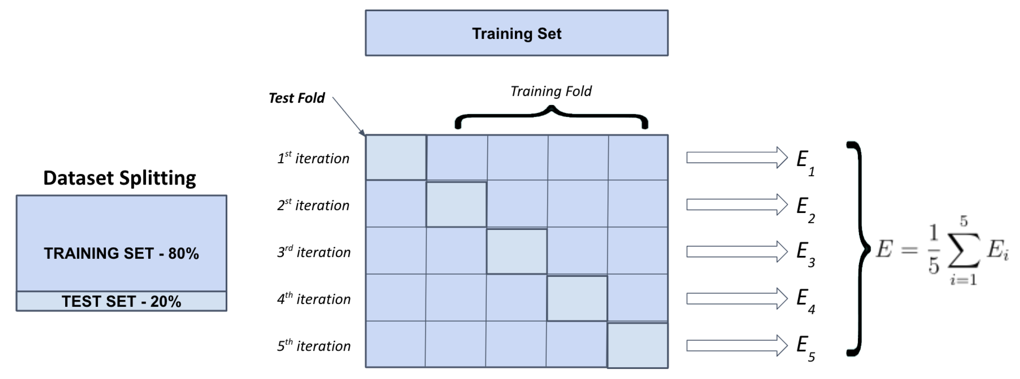
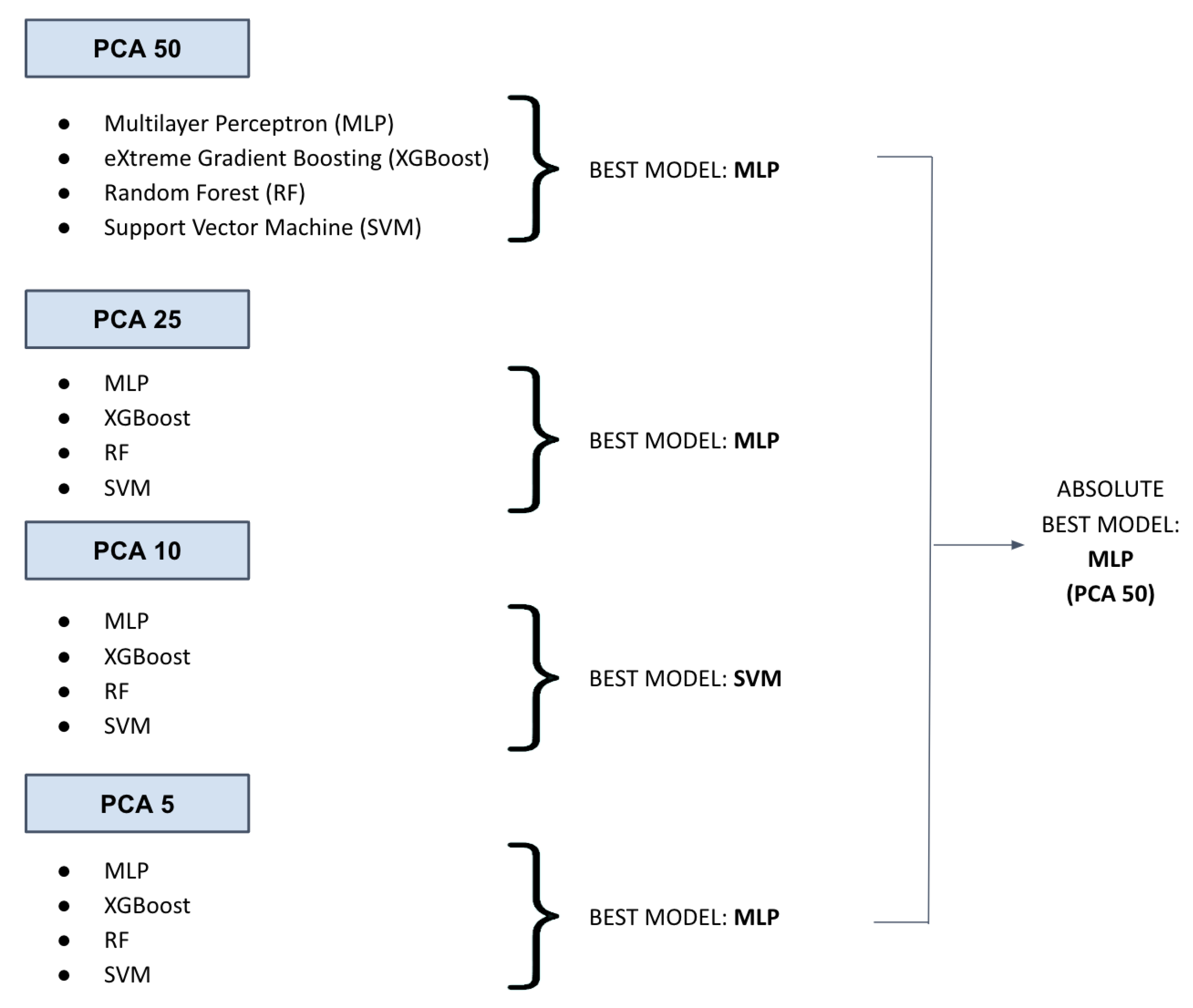
3.6. Data Splitting and Dimensionality Reduction

The whole dataset consisted of 6500 columns, given by 13 features times 500 samples, for 126 records, given by 21 athletes executing two times the three exercises. The dataset was split into training and test sets. The split percentages were $80\%$ for the training set and $20\%$ for the test set. The split was developed by exploiting the train_test_split function from Scikit-learn v1.0.2 library [38] with Python 3.9.0.

Since the dataset is affected by the curse of dimensionality, we applied principal component analysis (PCA) [39] to reduce the number of samples incrementally for each feature. Hence, we first made a train/test split, then fit the PCA with the training set and transformed both the training set and the test set with the fitted PCA. It is worth noting that, for each feature, every group of 500 samples was individually taken and reduced with PCA as follows:

• $k=50$, for an overall of 650 total features;
• $k=25$, for an overall of 325 total features;
• $k=10$, for an overall of 130 total features;
• $k=5$, for an overall of 65 total features.

The reduction has been developed by exploiting the Scikit-learn v1.0.2 library, feeding in input $\mathtt{n}\_\mathtt{components}=k$. Therefore, four training and test sets have been produced.

3.7. Machine Learning Algorithms

In order to determine the best classifier to predict the athlete class (novice or élite), we analyzed the following models:

• eXtreme Gradient Boosting (XGBoost) classifier [40]. The most crucial factor behind the success of XGBoost is its scalability in all scenarios due to several essential systems and algorithmic optimizations. It is an ensemble of K classification and regression trees (CART) $\left\{{\mathrm{T}}_1\left(x_i,y_i\right)\dots {\mathrm{T}}_K\left(x_i,y_i\right)\right\}$, where $x_i$ is the given training set of descriptors associated with a prediction of the class label, $y_i$. A CART assigns a real score to every leaf (outcome or target), so a combination of all prediction scores is used to get the final score, as indicated in ${\widehat{y}}_i={\sum }_{k=1}^K{f}_k\left(x_i\right),f_k\in F$. $f_k$ represents an independent tree structure with leaf scores, and F represents the space of all CARTs. This objective is defined as follows: $Obj\left(\mathsf{\Theta }\right)={\sum }_i^{n}l\left(y_i,{\widehat{y}}_i\right)+{\sum }_k^K\mathsf{\Omega }\left(f_k\right)$. In the first term, we have a differentiable loss function, l, which measures the difference between $\widehat{y}$ and $y_i$ before prediction. The second regularization term, $\mathsf{\Omega }$, penalizes the complexity of the model to avoid overfitting, and it is provided by $\mathsf{\Omega }\left(f\right)=\gamma T+\frac{1}{2}\lambda {\sum }_{j-1}^T{w}_j^2$. A leaf score is determined by the number of leafs T and the number of leafs w. The constants $\gamma$ and $\lambda$ control how much regularization occurs. Using regularization, shrinkage, and descriptor subsampling are additional methods of preventing overfitting.
• Multilayer Perceptron (MLP) [41]. It is a supervised learning algorithm that uses a feed-forward neural network technique. It consists of a layer of input, a hidden layer of threshold logic units (TLUs), and a layer of output. The hidden layers are all connected, and each TLU computes a weighted sum of its inputs before applying an activation function to provide a result that will be used as input for the next layer. Generally, activation functions are not linear and can take on $C\ast$1-differential forms. Back-propagation algorithms are based on making predictions and measuring performance (error) for every training instance. Thus, each layer is reversed to assess the contribution of each connection to the error; then, edge weights are modified to improve performance.
• Random forest (RF) classifier [42]. It is one of the best classifiers in terms of predictability and efficiency for high-dimensional datasets. It is a supervised learning algorithm based on constructing a collection of decision trees. For prediction, the RF model produces a variety of decision trees in the training phase, intending to reduce the variance of the final result by determining the class predicted most commonly by each tree within the forest. RF training algorithm consists of incorporating bootstrap aggregation to trees under training. $(X,Y)$ denotes the pair of training set X and target vector Y, where $X=\{x_1,\dots ,x_n\}$, and $Y=y_1,\dots ,y_n$. By replacing a random sample from X with a repeated (B times) extraction, the trees are fitted to this sample and repeated. In particular, for $b=1,\dots ,B$, the procedure is as follows: (1) Random sampling with replacement of n observations from the training set X to obtain $(X_b,Y_b)$ subsets. To reduce the correlation between trees originating from bagging, the cardinality of the subset is usually of order $\sqrt{p}$ for a classification problem with p features. Step (2) involves training the tree $f_b$ on $(X_b,Y_b)$. (3) Out-of-sample prediction on unseen dataset $x^{*}$ is the response outcome resulting from most of the results generated from every single tree. The number of trees in the forest is the free parameter of the model, usually set to at least ${10}^2$.
• Support Vector Machine (SVM) classifier [43]. The SVM is a supervised learning algorithm based on the concept of optimal hyper-planes that separate observations belonging to two different classes. Assuming that n points belong to two linearly separable sets in p-dimensional space, the goal of the linear classification problem is to find a (p-1)-dimensional hyperplane that can classify two classes with the most extensive margins, e.g., the most significant distance from the nearest points in each set to the boundary. In cases where the original data cannot be linearly separable, one possibility is to map the original data onto a higher-dimensional feature space to achieve more effective separation. Hence, support vector classifiers are generalized linear classifiers based on an “augmented” feature space with significantly high dimensionality. Suppose the transformed feature vectors $h\left(x\right)$ are given by the function $h\left(x\right)$. In that case, the optimization problem can easily be transformed into a quadratic programming problem using Lagrange multipliers in which the transformed vectors are scalar products. Thanks to this trick, it is not important to know the transformation, but only the type of the kernel function $K(x,x^{\prime })=\langle h\left(\mathbf{x}\right),h\left({\mathbf{x}}^{\prime }\right)\rangle$. The selection of a kernel function and the regularization parameter C determine the configuration of an SVM classifier. The following functions were chosen for the hyper-parameter tuning phase: (1) $d—$degree polynomials: $K(\mathbf{x},{\mathbf{x}}^{\prime })={(1+\langle \mathbf{x},{\mathbf{x}}^{\prime }\rangle )}^d$; (2) radial basis function (RBF): $K(\mathbf{x},{\mathbf{x}}^{\prime })=exp(-\gamma ||\mathbf{x}-{\mathbf{x}}^{\prime }{\left|\right|}^2)$, where values of parameters d, $\gamma$, ${\kappa }_1$, and ${\kappa }_2$ span specific ranges.

All four algorithms considered were supervised learning models. Afterward, a code was developed, and due to the interaction Python, it recalled the functions of the Machine Learning contained in the scikit-learn v1.0.2 library. This library was used to compare all models to identify the best suited to classify the élite and novice athletes and the model minimizing false-negative predictive values.

4. Results

In this section, we present and discuss the results of the experiments. Specifically, we compare the results obtained to identify the best model and the performances of the best model in Section 4.2. We discuss in Section 4.1 the metrics for evaluating Machine Learning models for classification modeling.

4.1. Evaluation Metrics

We adopted the metrics accuracy, precision, recall, and F1-score to evaluate the classification models’ performances. $TP$ represents the true positives, $TN$ represents the true negatives, $FP$ represents the false positives, and $FN$ represents the false negatives. According to Equation (3), accuracy is the ratio of correctly predicted observations to the total observations, and it represents how well the model performs across all classes. This value grows with a higher level of accuracy. In Equation (4), precision is defined as the ratio of correctly predicted positive observations to the total number of positively predicted observations. By measuring this metric, we can determine how accurate the model is at classifying samples as positive. In Equation (5), recall is calculated by dividing the number of positives correctly classified as positive by the total number of observations in the class. Observations that were correctly classified as positive indications that the model can detect them. Observations are detected more often when the recall is higher. Lastly, the F1-score in Equation (6) refers to the average precision and recall. Precision and recall must be $100\%$ to reach the maximum value of 1. Overall, the F1-score is a way to compare two models that predict the same variable.

$$\begin{array}{c}\hfill Accuracy=\frac{TP+TN}{TP+TN+FP+FN}\end{array}$$

(3)

$$\begin{array}{c}\hfill Precision=\frac{TP}{TP+FP}\end{array}$$

(4)

$$\begin{array}{c}\hfill Recall=\frac{TP}{TP+FN}\end{array}$$

(5)

$$\begin{array}{c}\hfill F1=2·\frac{Recall·Precision}{Recall+Precision}\end{array}$$

(6)

4.2. Best Model Performance Analysis

The algorithms were put through hyperparameter tuning to improve performance. For each model, the best parameters were chosen. The values of precision, recall, F1-score, macro-accuracy, and weighted accuracy were compared to identify the model with the best performance and the suitable trade-off between feature number and accuracy.

Table 2. Evaluation of best model for each k by various metrics.

Model	k	Accuracy	Average	Precision	Recall	F1-Score
MLP	5	0.88	macro	0.87	0.88	0.88
			weighted	0.88	0.88	0.88
SVM	10	0.84	macro	0.83	0.83	0.83
			weighted	0.84	0.84	0.84
MLP	25	0.84	macro	0.83	0.83	0.83
			weighted	0.84	0.84	0.84
MLP	50	0.92	macro	0.92	0.92	0.92
			weighted	0.92	0.92	0.92

summarizes the values of the metrics of the classifiers.

Using these metrics, we determined that the MLP algorithm with k = 50 was the best model.

4.3. Best Model Hyperparameter Tuning

The best model, i.e., MLP, was tuned using a GridSearchCV function in Python with a 5-fold cross-validation strategy to improve the model performance. GridSearchCV is included in the scikit-learn library. We performed the MLP optimization for the following parameters:

• hidden_layer_sizes’: [(sp_randint.rvs(100, 600, 1), sp_randint.rvs(100, 600, 1),),
  (sp_randint.rvs(100, 600, 1),)]
• activation: tanh, relu, logistic;
• solver: sgd, adam, lbfgs;
• alpha: 0.0001, 0.001, 0.01, 0.1, 0.9;
• learning_rate: "constant", "adaptive".

The values obtained at the end of the MLP optimization were:

• hidden_layer_sizes: (586);
• activation: relu;
• solver: lbfgs;
• alpha: 0.1;
• learning_rate: constant.

To evaluate the best predictive model, we considered the metrics of precision, recall, F1-score, and AUC.

Table 3. Metrics evaluation of MLP classifier.

Category	Precision	Recall	F1-Score
Novice (0)	$90\%$	$90\%$	$90\%$
élite (1)	$93\%$	$93\%$	$93\%$

shows the performance of the MLP algorithm in predicting the fencer class (élite/Novice). In addition, the confusion matrix (CM) was evaluated to highlight the number of fencers misclassified during the testing phase.

4.4. Experimental Setup

To summarize what is described in the previous sections (Section 4.2 and Section 4.3) and make explicit the techniques applied, the steps performed are described below:

• Raw data acquisition of the signal;
• Creating the dataset through preprocessing;
• Applying PCA to the preprocessed data (k is determined based on the best model);
• The ML algorithm performs the prediction using the data described in the previous step.

Figure 4, summarises the splitting operations performed during the experiments.

The first operation was to perform dataset splitting of 80/20. The test set partition was kept aside and was not used in the analysis. The train set partition was used for a k-fold cross validation analysis [44].

In k-fold cross-validation, we randomly split the training dataset into k folds without replacement, where k-1 folds were used for the model training, and one fold was used for performance evaluation. This procedure was repeated k times to obtain k models and performance estimates. We then calculated the average performances of the models based on the different independent folds to obtain a performance estimate that is less sensitive to the training data’s sub-partitioning than the holdout method. Typically, we use k-fold cross-validation for model tuning, finding the optimal hyperparameter values that yield a satisfying generalization performance. Once we have found satisfactory hyperparameter values, we can retrain the model on the complete training set and obtain a final performance estimate using the independent test set. The rationale behind fitting a model to the whole training dataset after k-fold cross-validation is that providing more training samples to a learning algorithm usually results in a more accurate and robust model.

In particular, in our work, the training dataset was divided into five folds, and during the 5 iterations, four folds were used for training, and one fold was used as the test set for the model evaluation. The estimated performances $E_i$ (for example, classification accuracy or error) for each fold were then used to calculate the estimated average performance E of the model. Regarded k-fold cross validation, hyperparameter tuning analysis was carried out on each proposed classifier under study (Section 3.7), to identify the best hyperparameters. For each PCA value, five best models were identified. Each of these were compared with the identified best models of the other PCAs. The absolute best model, and the corresponding k-value (PCA), were then identified.

Figure 5 below, shows the approach previously described:

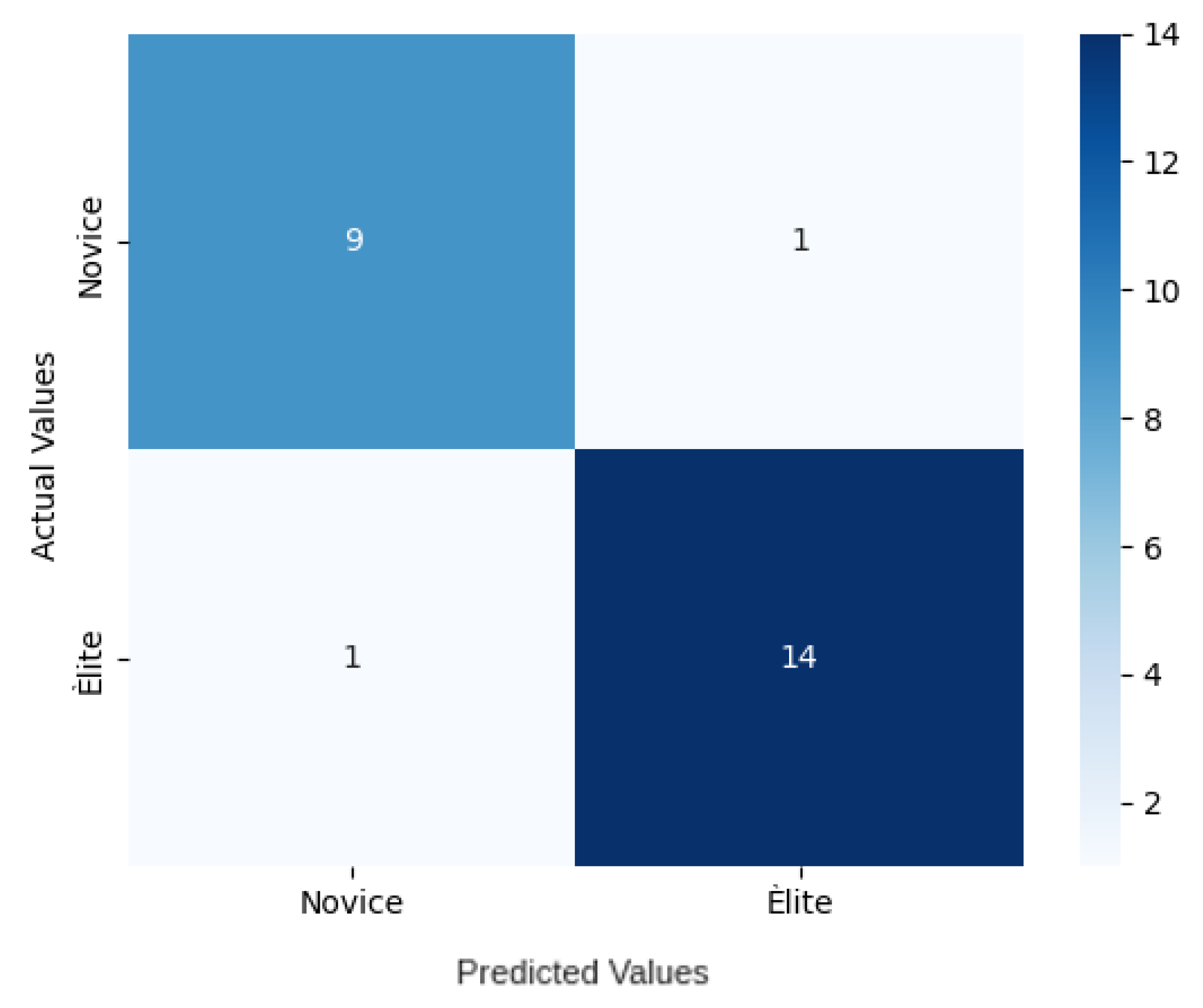
4.5. Performance Evaluation of the Absolute Best Model

The first parameter considered to investigate the performance of MLP carefully was accuracy.

The accuracy of the MLP was measured during the training and testing phases. The training accuracy was $100\%$, and the test accuracy was $96.0\%$.

Another performance index that we considered was the value of the area under the ROC (AUC, Area Under the Curve) [45], which is a measure of accuracy and indicates the diagnostic power of the test.

Figure 6 shows the ROC curves with the AUC value obtained during the testing phase. In addition to the accuracy and ROC curve values, we evaluated the confusion matrix to ensure the reliability of the MLP. Figure 7 shows the confusion matrix values from the test phase.

The values obtained for AUC and accuracy show that the MLP implemented did not present overfitting or underfitting problems because the values of the two ROC curves and the values related to the accuracy differ very slightly. Additionally, to validate the MLP precision’s performance, recall and F1-score values during the test phase were evaluated. In Table 3, are shown values of precision, recall, and F1-score of novice fencers and élite fencers during the test phase.

5. Concluding Remarks and Perspectives

To investigate and analyze sports movement, it is necessary to understand its nature and goal and to identify the factors that affect its performance. In the present work, we exploited Machine Learning techniques to support fencing training using acceleration, angular velocities, pelvis angles, and four sEMG signals to classify different levels of expertise (élite and novice fencers). Our study searched for the best algorithm to support fencing training by comparing each model’s different Machine Learning algorithms. The ML algorithm with the highest accuracy was subjected to hyperparameter tuning for each dataset. From this procedure, as it is possible to see from the presented results, the best model was the Multilayer Perceptron (MLP), in Python, for the dataset with 650 total features. The MLP makes very few mistakes, and it can predict the outcome with high accuracy. The model has a slightly higher capacity for recognizing élite fencers than novice; this is important to determine which training plan and execution are the best to achieve good performance in the lunge execution so that good results are had during competitions.

In all sports, accurate and proper training planning and execution are essential to success. In order to verify training results, it is good to perform a biomechanical study of the primary and most used technical gesture during a competition. Furthermore, understanding a sport’s biomechanics and requirements paves the way for injury prevention and safety enhancement [26]. Previous studies have focused on the application of ML algorithms to classify different tasks (i.e., fencers’ footwork [37]; lunge phases [35]) or reduce the number of sensors to be considered. Our approach stemmed from the idea that combining different biosignals (acceleration, angular velocities, pelvis angles, muscle activities) could be more useful in proposing a framework for fencing training. Using wearable technologies, raw data can be easily generated and collected. These data, after appropriate processing, provide essential information on the execution of movements, allowing us to determine whether the gesture is correctly performed. As a result, athletes could enhance their skills, strategies, overall performance, and competitiveness. The use of these new methods enjoys several fundamental properties: (i) they can find hidden relationships between variables used for training Machine Learning models; (ii) they allow for easier handling of large amounts of data; and (iii) they can be integrated within software platforms that allow for capturing, in our case, biomechanical data in real-time used to provide a rapid prediction of outcome and thus direct feedback to the trainer and athlete.

The way humans move and the underlying cognitive control involved in this process is inherently complex, dynamic, multidimensional, and highly non-linear. Machine Learning approaches enable us to embrace this complexity, working on three complementary tasks: predictive modeling, classification, and dimensionality reduction [46]. In particular, the automatic classification of athletic tasks based on motion data gathered in real-world conditions with inertial sensors is another expanding area of investigation, as demonstrated by the research studies carried out in the field. Furthermore, Hammes and colleagues [47] performed a narrative review that explored the role of AI in élite sports. They showed that most activities were carried out in signal and image processing methodical categories. However, projects in the field of modeling and planning have become increasingly popular in the last few years. Based on these two perspectives, they extracted deficits, issues, and opportunities and summarized them in six key challenges faced by the sports analytics community. These challenges include data collection, the practitioners’ controllability of AI results, and the explainability of AI results [47]. Future investigations will provide quantitative criteria and optimum patterns by studying and extracting the kinematics of successful fencers’ motions, which could be used to train beginners. Using AI could allow for novel solutions when optimizing plans and strategies. Exploring new solutions and exploiting proven ones will determine a parameterization dimension that systematically allows coaches and athletes to match opportunities and risks.

References

- Chen, T.L.W.; Wong, D.W.C.; Wang, Y.; Ren, S.; Yan, F.; Zhang, M. Biomechanics of fencing sport: A scoping review. PLoS ONE 2017, 12, e0171578. [Google Scholar] [CrossRef] [Green Version]
- Sorel, A.; Plantard, P.; Bideau, N.; Pontonnier, C. Studying fencing lunge accuracy and response time in uncertain conditions with an innovative simulator. PLoS ONE 2019, 14, e0218959. [Google Scholar] [CrossRef]
- Bottoms, L.; Greenhalgh, A.; Sinclair, J. Kinematic determinants of weapon velocity during the fencing lunge in experienced épée fencers. Acta Bioeng. Biomech. 2013, 15, 4. [Google Scholar]
- Camomilla, V.; Bergamini, E.; Fantozzi, S.; Vannozzi, G. Trends supporting the in-field use of wearable inertial sensors for sport performance evaluation: A systematic review. Sensors 2018, 18, 873. [Google Scholar] [CrossRef] [Green Version]
- Bortone, I.; Moretti, L.; Bizzoca, D.; Caringella, N.; Delmedico, M.; Piazzolla, A.; Moretti, B. The importance of biomechanical assessment after Return to Play in athletes with ACL-Reconstruction. Gait Posture 2021, 88, 240–246. [Google Scholar] [CrossRef]
- Ardito, C.; Di Noia, T.; Di Sciascio, E.; Lofú, D.; Mallardi, G.; Pomo, C.; Vitulano, F. Towards a trustworthy patient home-care thanks to an edge-node infrastructure. In Proceedings of the International Conference on Human-Centred Software Engineering, Eindhoven, The Netherlands, 24–26 August 2020; Springer: Berlin/Heidelberg, Germany, 2020; pp. 181–189. [Google Scholar]
- Pazienza, A.; Anglani, R.; Mallardi, G.; Fasciano, C.; Noviello, P.; Tatulli, C.; Vitulano, F. Adaptive Critical Care Intervention in the Internet of Medical Things. In Proceedings of the 2020 IEEE International Conference on Evolving and Adaptive Intelligent Systems (EAIS), Bari, Italy, 27–29 May 2020; pp. 1–8. [Google Scholar]
- Ardito, C.; Di Noia, T.; Fasciano, C.; Lofú, D.; Macchiarulo, N.; Mallardi, G.; Pazienza, A.; Vitulano, F. Management at the Edge of Situation Awareness during Patient Telemonitoring. In Proceedings of the 19th International Conference of the Italian Association for Artificial Intelligence (AIxIA 2020), Virtually, 25–27 November 2020; Springer: Berlin/Heidelberg, Germany, 2021; Volume 12414, pp. 372–387. [Google Scholar]
- Ardito, C.; Di Noia, T.; Fasciano, C.; Lofú, D.; Macchiarulo, N.; Mallardi, G.; Pazienza, A.; Vitulano, F. Towards a Situation Awareness for eHealth in Ageing Society. In Proceedings of the Italian Workshop on Artificial Intelligence for an Ageing Society (AIxAS 2020), Virtually, 25–27 November 2020; pp. 40–55. [Google Scholar]
- Ardito, C.; Di Noia, T.; Di Sciascio, E.; Lofú, D.; Pazienza, A.; Vitulano, F. User Feedback to Improve the Performance of a Cyberattack Detection Artificial Intelligence System in the e-Health Domain. In Proceedings of the Human–Computer Interaction—INTERACT 2021, Bari, Italy, 30 August–3 September 2021; pp. 295–299. [Google Scholar]
- Ardito, C.; Di Noia, T.; Di Sciascio, E.; Lofù, D.; Pazienza, A.; Vitulano, F. An Artificial Intelligence Cyberattack Detection System to Improve Threat Reaction in e-Health. In Proceedings of the ITASEC, Virtually, 7–9 April 2021. [Google Scholar]
- Ardito, C.; Bellifemine, F.; Di Noia, T.; Lofú, D.; Mallardi, G. A proposal of case-based approach to clinical pathway modeling support. In Proceedings of the 2020 IEEE Conference on Evolving and Adaptive Intelligent Systems (EAIS), Bari, Italy, 27–29 May 2020; pp. 1–6. [Google Scholar]
- Sorino, P.; Caruso, M.G.; Misciagna, G.; Bonfiglio, C.; Campanella, A.; Mirizzi, A.; Franco, I.; Bianco, A.; Buongiorno, C.; Liuzzi, R.; et al. Selecting the best machine learning algorithm to support the diagnosis of Non-Alcoholic Fatty Liver Disease: A meta learner study. PLoS ONE 2020, 15, e0240867. [Google Scholar] [CrossRef]
- Lella, E.; Pazienza, A.; Lofú, D.; Anglani, R.; Vitulano, F. An Ensemble Learning Approach Based on Diffusion Tensor Imaging Measures for Alzheimer’s Disease Classification. Electronics 2021, 10, 249. [Google Scholar] [CrossRef]
- Tatoli, R.; Lampignano, L.; Bortone, I.; Donghia, R.; Castellana, F.; Zupo, R.; Tirelli, S.; De Nucci, S.; Sila, A.; Natuzzi, A.; et al. Dietary Patterns Associated with Diabetes in an Older Population from Southern Italy Using an Unsupervised Learning Approach. Sensors 2022, 22, 2193. [Google Scholar] [CrossRef]
- Pazienza, A.; Anglani, R.; Fasciano, C.; Tatulli, C.; Vitulano, F. Evolving and Explainable Clinical Risk Assessment at the Edge. Evol. Syst. 2022, 1–20. [Google Scholar] [CrossRef]
- Lofú, D.; Pazienza, A.; Ardito, C.; Di Noia, T.; Di Sciascio, E.; Vitulano, F. A Situation Awareness Computational Intelligent Model for Metabolic Syndrome Management. In Proceedings of the 2022 IEEE Conference on Cognitive and Computational Aspects of Situation Management (CogSIMA), Salerno, Italy, 6–10 June 2022; pp. 118–124. [Google Scholar] [CrossRef]
- Pazienza, A.; Monte, D. Introducing the Monitoring Equipment Mask Environment. Sensors 2022, 22, 6365. [Google Scholar] [CrossRef]
- Sorino, P.; Campanella, A.; Bonfiglio, C.; Mirizzi, A.; Franco, I.; Bianco, A.; Caruso, M.G.; Misciagna, G.; Aballay, L.R.; Buongiorno, C.; et al. Development and validation of a neural network for NAFLD diagnosis. Sci. Rep. 2021, 11, 20240. [Google Scholar] [CrossRef] [PubMed]
- Ardito, C.; Di Noia, T.; Fasciano, C.; Lofù, D.; Macchiarulo, N.; Mallardi, G.; Pazienza, A.; Vitulano, F. An Edge Ambient Assisted Living Process for Clinical Pathway. In Ambient Assisted Living; Bettelli, A., Monteriù, A., Gamberini, L., Eds.; Springer International Publishing: Cham, Switzerland, 2022; pp. 363–374. [Google Scholar]
- Mawgoud, A.; Abu-Talleb, A.; El Karadawy, A.; Eltabey, M. The Appliance of Artificial Neural Networks in Fencing Sport Via Kinect Sensor; ResearchGate: Berlin, Germany, 2016. [Google Scholar] [CrossRef]
- Timpka, T.; Ekstrand, J.; Svanström, L. From sports injury prevention to safety promotion in sports. Sport. Med. 2006, 36, 733–745. [Google Scholar] [CrossRef] [PubMed]
- Bai, D.; Liu, T.; Han, X.; Yi, H. Application research on optimization algorithm of sEMG gesture recognition based on light CNN+ LSTM model. Cyborg Bionic Syst. 2021, 2021. [Google Scholar] [CrossRef]
- Alhasan, H.S.; Wheeler, P.C.; Fong, D.T. Application of interactive video games as rehabilitation tools to improve postural control and risk of falls in prefrail older adults. Cyborg Bionic Syst. 2021, 2021. [Google Scholar] [CrossRef]
- Guan, Y.; Guo, L.; Wu, N.; Zhang, L.; Warburton, D.E. Biomechanical insights into the determinants of speed in the fencing lunge. Eur. J. Sport Sci. 2018, 18, 201–208. [Google Scholar] [CrossRef]
- Turner, A.; James, N.; Dimitriou, L.; Greenhalgh, A.; Moody, J.; Fulcher, D.; Mias, E.; Kilduff, L. Determinants of Olympic fencing performance and implications for strength and conditioning training. J. Strength Cond. Res. 2014, 28, 3001–3011. [Google Scholar] [CrossRef]
- Suchanowski, A.; Boryszewski, Z.; Pakosz, P. Electromyography signal analysis of the fencing lunge by Magda Mroczkiewicz, the leading world female competitor in foil. Balt. J. Health Phys. Act. 2011, 3, 4. [Google Scholar] [CrossRef]
- Gholipour, M.; Tabrizi, A.; Farahmand, F. Kinematics analysis of lunge fencing using stereophotogrametry. World J. Sport Sci. 2008, 1, 32–37. [Google Scholar]
- Borysiuk, Z. Type of perception vs. lunge in fencing technique structure. Rev. Artes Marciales Asiát. 2016, 11, 36–37. [Google Scholar] [CrossRef] [Green Version]
- Gutierrez-Davila, M.; Rojas, F.J.; Antonio, R.; Navarro, E. Response timing in the lunge and target change in elite versus medium-level fencers. Eur. J. Sport Sci. 2013, 13, 364–371. [Google Scholar] [CrossRef] [PubMed]
- Gutiérrez-Dávila, M.; Rojas, F.J.; Caletti, M.; Antonio, R.; Navarro, E. Effect of target change during the simple attack in fencing. J. Sport. Sci. 2013, 31, 1100–1107. [Google Scholar] [CrossRef] [Green Version]
- Borysiuk, Z.; Markowska, N.; Niedzielski, M. Analysis of the fencing lunge based on the response to a visual stimulus and a tactile stimulus. J. Combat Sport. Martial Arts 2014, 5, 117–122. [Google Scholar] [CrossRef] [Green Version]
- Borysiuk, Z.; Piechota, K.; Minkiewicz, T. Analysis of performance of the fencing lunge with regard to the difficulty level of a technical-tactical task. J. Combat. Sport. Martial Arts 2013, 4, 135–139. [Google Scholar] [CrossRef] [Green Version]
- Richter, C.; O’Reilly, M.; Delahunt, E. Machine learning in sports science: Challenges and opportunities. Sport. Biomech. 2021, 1–7. [Google Scholar] [CrossRef]
- Malawski, F. Depth versus inertial sensors in real-time sports analysis: A case study on fencing. IEEE Sens. J. 2020, 21, 5133–5142. [Google Scholar] [CrossRef]
- O’Reilly, M.A.; Whelan, D.F.; Ward, T.E.; Delahunt, E.; Caulfield, B. Classification of lunge biomechanics with multiple and individual inertial measurement units. Sport. Biomech. 2017, 16, 342–360. [Google Scholar] [CrossRef]
- Malawski, F.; Kwolek, B. Classification of basic footwork in fencing using accelerometer. In Proceedings of the 2016 Signal Processing: Algorithms, Architectures, Arrangements, and Applications (SPA), Poznan, Poland, 21–23 September 2016; pp. 51–55. [Google Scholar]
- Pedregosa, F.; Varoquaux, G.; Gramfort, A.; Michel, V.; Thirion, B.; Grisel, O.; Blondel, M.; Prettenhofer, P.; Weiss, R.; Dubourg, V.; et al. Scikit-learn: Machine learning in Python. J. Mach. Learn. Res. 2011, 12, 2825–2830. [Google Scholar]
- Fodor, I.K. A Survey of Dimension Reduction Techniques; Technical Report; Lawrence Livermore National Lab.: Livermore, CA, USA, 2002. [Google Scholar]
- Chen, T.; Guestrin, C. Xgboost: A scalable tree boosting system. In Proceedings of the 22nd ACM Sigkdd International Conference on Knowledge Discovery and Data Mining, San Francisco, CA, USA, 13–17 August 2016; pp. 785–794. [Google Scholar]
- Hinton, G.E. Connectionist learning procedures. In Machine Learning, Volume III; Elsevier: Amsterdam, The Netherlands, 1990; pp. 555–610. [Google Scholar]
- Breiman, L. Random forests. Mach. Learn. 2001, 45, 5–32. [Google Scholar] [CrossRef] [Green Version]
- Cortes, C.; Vapnik, V. Support-vector networks. Mach. Learn. 1995, 20, 273–297. [Google Scholar] [CrossRef]
- Refaeilzadeh, P.; Tang, L.; Liu, H. Cross-validation. Encycl. Database Syst. 2009, 5, 532–538. [Google Scholar]
- Bradley, A.P. The use of the area under the ROC curve in the evaluation of machine learning algorithms. Pattern Recognit. 1997, 30, 1145–1159. [Google Scholar] [CrossRef] [Green Version]
- Zago, M.; Kleiner, A.F.R.; Federolf, P.A. Machine learning approaches to human movement analysis. Front. Bioeng. Biotechnol. 2021, 1573. [Google Scholar] [CrossRef]
- Hammes, F.; Hagg, A.; Asteroth, A.; Link, D. Artificial intelligence in elite sports—A narrative review of success stories and challenges. Front. Sport. Act. Living 2022, 4, 861466. [Google Scholar] [CrossRef]