
Clustering-Based Segmented Regression for Particulate Matter Sensor Calibration
1
College of Information Science and Engineering, Guilin University of Technology, Guilin 541004, China
2
Guangxi Key Laboratory of Embedded Technology and Intelligent System, Guilin University of Technology, Guilin 541004, China
3
Shenzhen International Graduate School, Tsinghua University, Shenzhen 518055, China
*
Author to whom correspondence should be addressed.
Appl. Sci. 2022, 12(24), 12934; https://doi.org/10.3390/app122412934
Submission received: 20 October 2022
/
Revised: 23 November 2022
/
Accepted: 2 December 2022
/
Published: 16 December 2022
(This article belongs to the Special Issue Information Fusion and Its Applications for Smart Sensing)
Abstract
:Nowadays, sensor-based air pollution sensing systems are widely deployed for fine-grained pollution monitoring. In-field calibration plays an important role in maintaining sensory data quality. Determining the model structure is challenging using existing methods of variable global fitting models for in-field calibration. This is because the mechanism of interference factors is complex and there is often insufficient prior knowledge on a specific sensor type. Although Artificial-Neuron-Net-based (ANN-based) methods ignore the complex conditions above, they also have problems regarding generalization, interpretability, and calculation cost. In this paper, we propose a clustering-based segmented regression method for particulate matter (PM) sensor in-field calibration. Interference from relative humidity and temperature are taken into consideration in the particulate matter concentration calibration model. Samples for modeling are divided into clusters and each cluster has an individual multiple linear regression equation. The final calibrated result of one sample is calculated from the regression model of the cluster the sample belongs to. The proposed method is evaluated under in-field deployment and performs better than a global multiple regression method both on PM and PM pollutants with, respectively, at least 16% and 9% improvement ratio on RMSE error. In addition, the proposed method is insensitive to reduction of training data and increase in cluster number. Moreover, it may bear lighter calculation cost, less overfitting problems and better interpretability. It can improve the efficiency and performance of post-deployment sensor calibration.
1. Introduction
Recently, serious issues concerning air pollution have raised public attention with the development of urbanization and industrialization [1]. It presents a severe threat to not only the ecological environment but also to human health. In order to improve the environmental monitoring and governance capacity, high-precision air pollution monitoring stations are established all over the world to obtain accurate air pollutant concentration information [2]. However, monitoring stations cannot be deployed with a high-spatial density to achieve high resolution because it is limited by large costs associated with high-precision equipment [3,4].
For fine-grained monitoring, various forms of wireless sensor networks (WSN) have been applied in air pollution monitoring as a complement [5,6,7,8]. Low-cost gas or particulate sensors make fine-grained air pollution monitoring possible under large-scale deployment. Compared with existing monitoring architecture with high-precision equipment, sensor-based air pollution monitoring has high resolution both spatially and temporally [9] at the expense of accuracy and robustness [10], due to limitations regarding the sensor’s characteristics and performance. First, sensor drift [11] and cross-sensitivity [11,12] inevitably cause measurement deviations after deployment. In addition, environmental factors such as temperature and humidity result in response fluctuations increasing measurement deviation further [13]. Therefore to guarantee the performance of a sensor-based air pollution monitoring system and make it closer to ground truth, it is essential to calibrate the sensory data against varied interference.
In this paper, we focus on in-field calibration problem of particulate matter (PM) sensor for PM and PM sensing and propose a clustering-based segmented regression method. Interference from relative humidity and temperature are taken into consideration in the particulate matter concentration calibration model. Instead of a global regression model covering all situations of concentration, and humidity and temperature, samples for modeling are divided into clusters by a clustering algorithm and each cluster has an individual multiple linear regression equation. After the calibration modeling mentioned above is finished, the final calibrated result of one sample is obtained from the regression model of the cluster the sample belongs to. Our method is evaluated under a practical in-field deployment and shown to perform better than a global multiple regression method under different initial error levels. It demonstrates at least 16% and 9% improvement ratio of calibration error on RMSE, respectively, for pollutants PM and PM than the baseline, especially when relative humidity is involved.
The main contributions of the paper are as follows. First, the clustering-based segmented regression method uses a combination of linear regression models to approximate a complex function structure for the in-field sensor calibration problem. It only relies on sensory data sampling with little prior knowledge of sensor characteristics. Second, the proposed method may have lower calculation cost and relieve overfitting problems, since its error is not overly sensitive to the cluster number and the ratio of training set and testing set. Third, it demonstrates better performance with a better fitting degree and a smaller calibration error both in mean value and variance, when compared with the global multiple linear regression model. Furthermore, it is easier to explain than those ANN-based methods.
2. Materials and Methods
2.1. Problem Background
Nowadays, the sensor-based air pollution sensing system has become a key complement to standardized air pollution monitoring architecture. Compared to conventional technologies with precision equipment, it provides fine-grained information in urban air pollution monitoring because low-cost sensors can support large-scale deployment. Meanwhile, it is acknowledged that low-cost sensors suffer from measurement performance limitations due to varied interference factors including sensor drift [14], working conditions (such as temperature and humidity) and cross-sensitivity [15].
To guarantee the quality of sensory data quality continuously, kinds of system-level sensor calibration methods are developed like collaborative calibration [16], blind calibration [17] and transfer calibration [18]. Although in-field calibration is a relatively basic technology, it still plays an important role in sensing system deployment because it has access to reliable reference from trusted standard monitoring station.
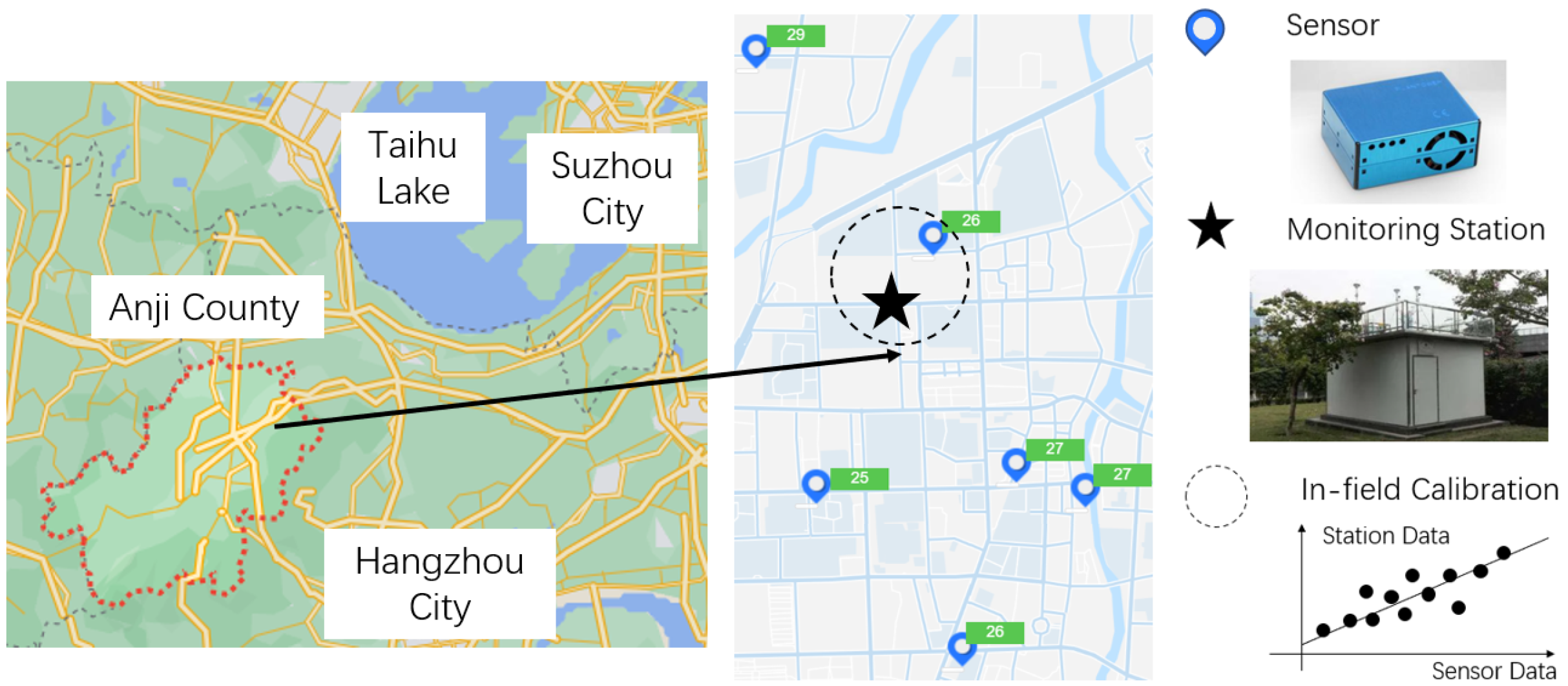
For example, as shown in Figure 1, in-field calibration can be conducted when the sensor is deployed in close proximity to the station providing trusted measurements as reference or ground truth. They are in co-location and bear common observation on environmental conditions in the same time period. In-field calibration centers on finding a fitting function or regression model that can estimate the ground truth from sensory data.
In detail, particulate matter monitoring is now a popular issue in urban atmosphere environment monitoring and PM sensors are widely used for sensing system deployment. Common PM sensors are based on optical principles and suffer from measurement deviations due to relative humidity and temperature. In-field calibration on PM sensors under practical working conditions will enhance sensor measurement performance with efficient deployment compared to pre-deployment calibration conducted under a laboratory setting. In essence, regarding sensory data as a series of input variables, the target of in-field PM sensor calibration is to find a function or model. It is then able to map these input variables to a ground truth estimation given by a standard monitoring station.
2.2. Related Work
In practice, sensor calibration faces challenges posed by sensor type variety and individual differences within the same sensor type [19]. Deployment of the sensing system requires high efficiency, and it is difficult to fully learn sensor’s characteristics under a controlled environment and figure out corresponding calibration model in laboratory calibration before deployment. Instead in-field calibration [20] make it possible to calibrate sensor under practical environment after deployment and improve sensor performance continuously.
Regression methods are widely applied in in-field sensor calibration against a series of measurement interference including drift [21], cross-sensitivity [19] and environment factors such as temperature and relative humidity [19]. One of the major challenges of in-field calibration is to determine the structure of regression model, since the mechanism of interference factors is complex and it is difficult to directly design a global fitting function for a specific sensor type based on prior knowledge, especially when there are non-linear responding characteristics [22]. In this case, simple linear [23,24] or multivariate linear regression [4,23] methods cannot perform well either on the whole range of the sensor or under some working conditions. Some ANN-based methods such as [25] use multi-layer back-propagation artificial neural network to consider the multiple environmental factors that affect low-cost air temperature sensors. In addition, random forest model is often used as a non-linear model for in-field calibration such as [26]. They may generate non-linear fitting function for calibration or achieve a relatively satisfying result, and its generalization performance, interpretability and calculation cost still remain bottlenecks for use across various in-field sensor calibration scenarios. For in-field sensor calibration, a regression is required to deal with sensor’s non-linear response characteristics under variable interference factors with small-scale training data and simple model structure.
2.3. Methodology Design
2.3.1. Motivation
Our proposed method is targeted at PM sensor in-field calibration to reduce deviations against relative humidity and temperature. Because the interference mechanism is difficult to describe under practical working conditions and individual differences exist among sensors, it is challenging to determine a global regression model to cover the whole sensor range and all common temperature and humidity situations. Even some methods such as ANN-based learning can fit any non-linear model theoretically, high complexity, generalization performance risk and large requirement on data amount limit their advantages.
Therefore, an intended in-field calibration model for PM sensor can compensate for deviation even with non-linear characteristics caused by relative humidity and temperature at a light calculation cost, together with interpretability and adaptability. Inspired by segmented linear regression, although it is difficult to directly find a global regression model to compensate varied deviation, linear regression still works in some local domains [26]. In fact, samples from sensory data can be divided into several parts and linear regression performs well in each part. The division can be realized via clustering algorithm adaptability [27].
2.3.2. Input Variables
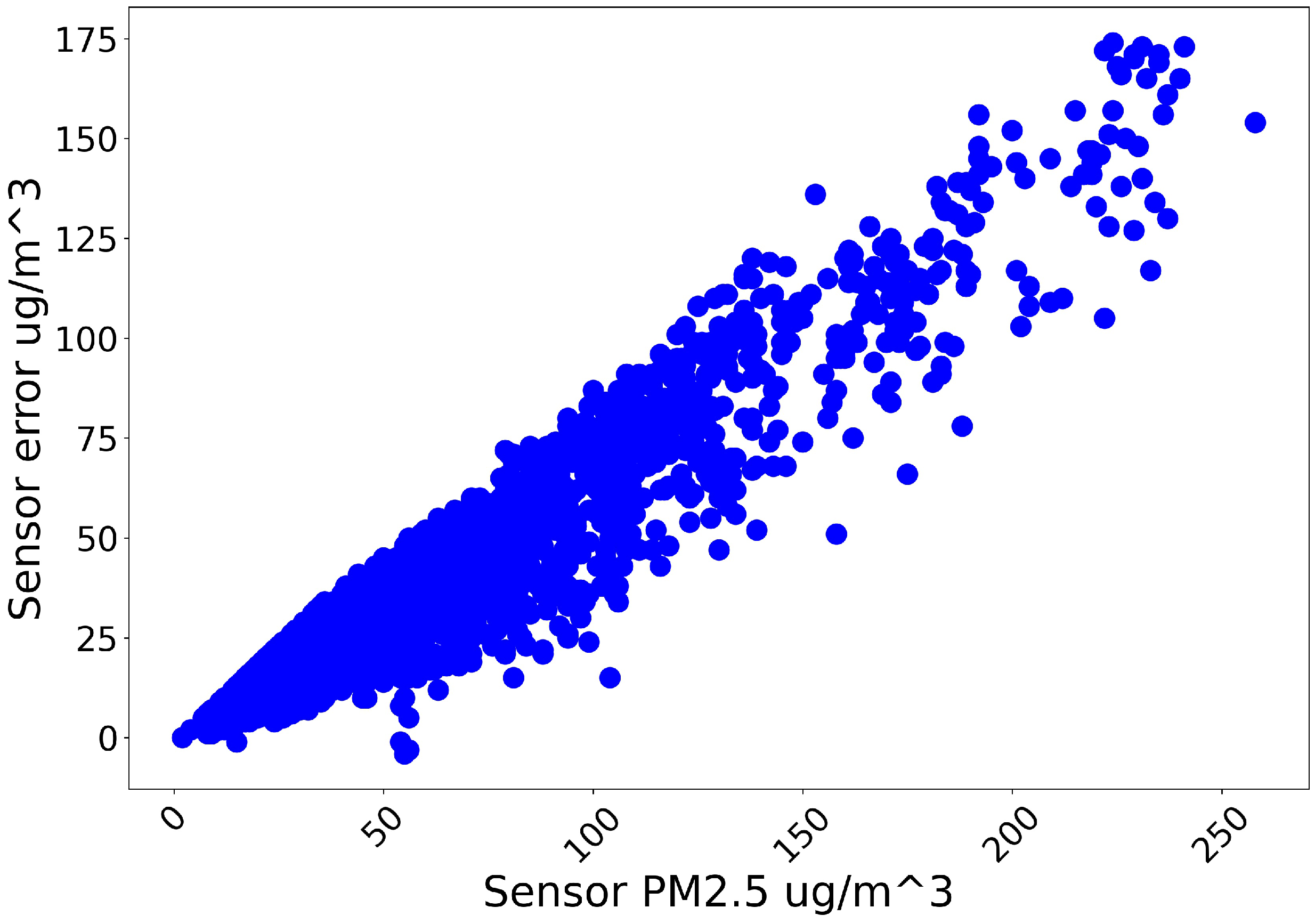
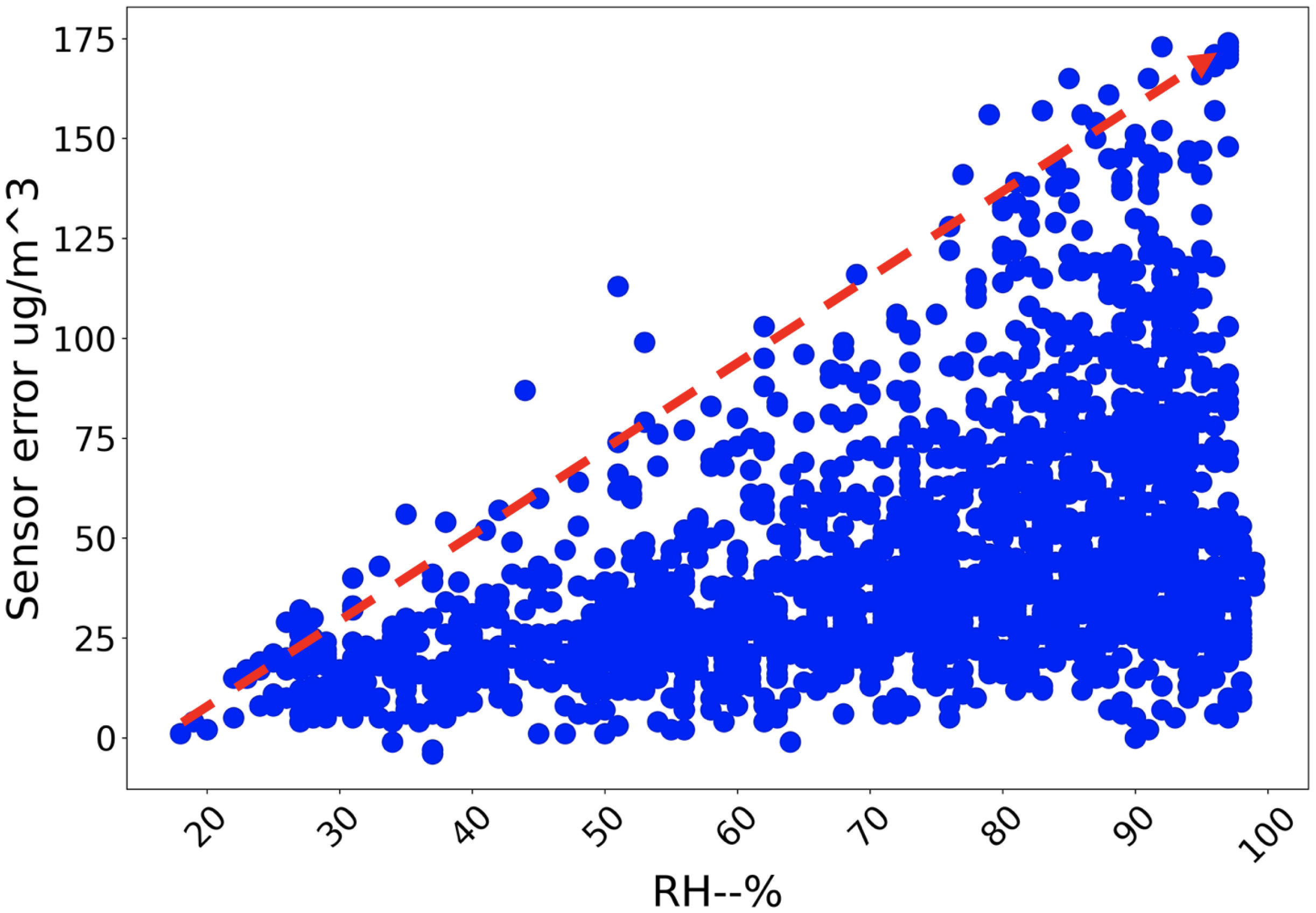
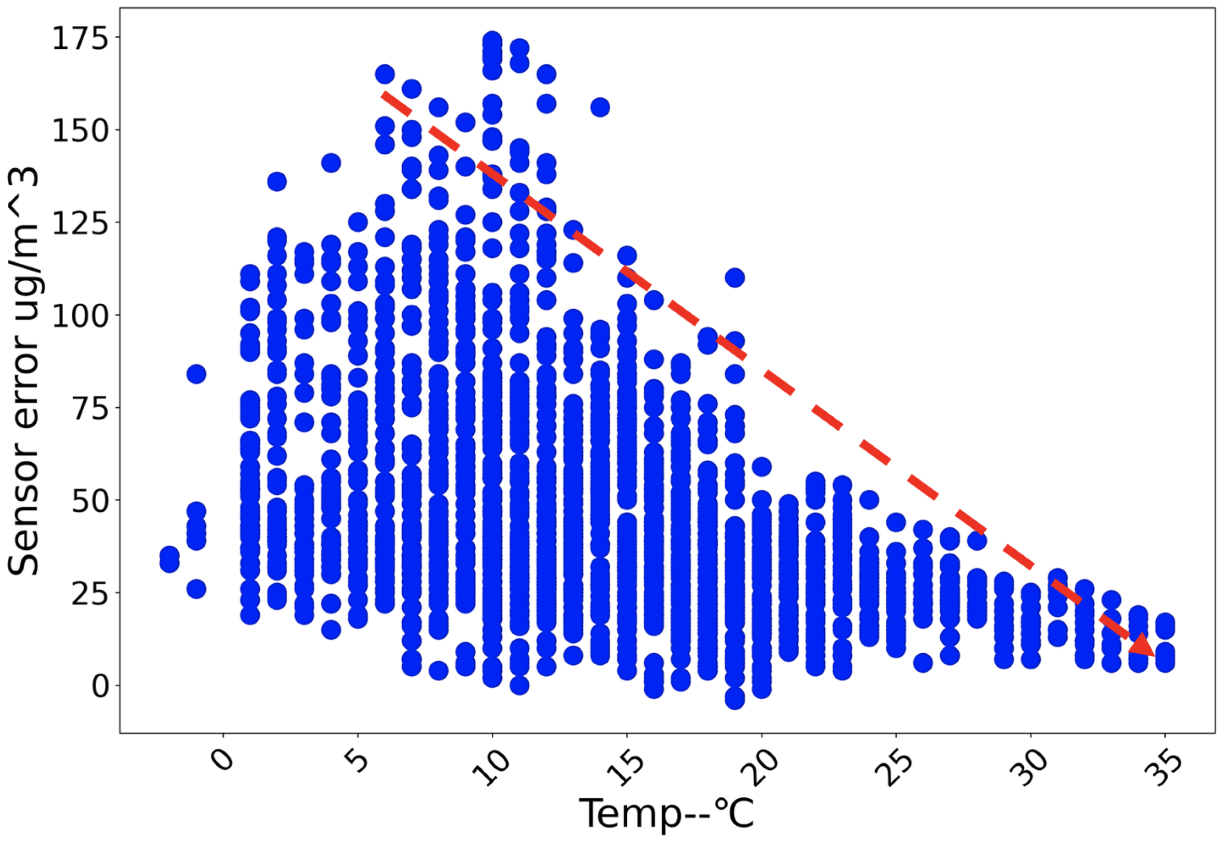
In our in-field calibration problem, input variables from the sensor taken into consideration for the calibration model include PM concentration, relative humidity and temperature, since we find the association between each variable and the error to be calibrated at an hourly scale. We define the ’error to be calibrated’ as the PM concentration deviation between sensor and reference station in co-location on an average hourly scale.
As shown in Figure 2, sensory PM concentration samples share a strong association with the error. That is because the sensor’s PM concentration reading shares a close trend with that of reference station on hourly average scale. When it comes to variable relative humidity and temperature, although their respective association with error is not as remarkable as concentration in Figure 3 and Figure 4, we also find that error’s upper bound may bear association with relative humidity or temperature. With regard to PM, we also find a similar association. So based on these three input variables, the calibration model has potential to compensate for sensory data errors.
2.3.3. Calibration Model
For PM sensor in-field calibration, our proposed method is clustering-based segmented regression. Sensory data of PM concentration, temperature and relative humidity are used to compensate measurement deviation and hourly PM concentration data from a standard monitoring station nearby are used as calibration reference. The method consists of two stages, modeling and calibrating.
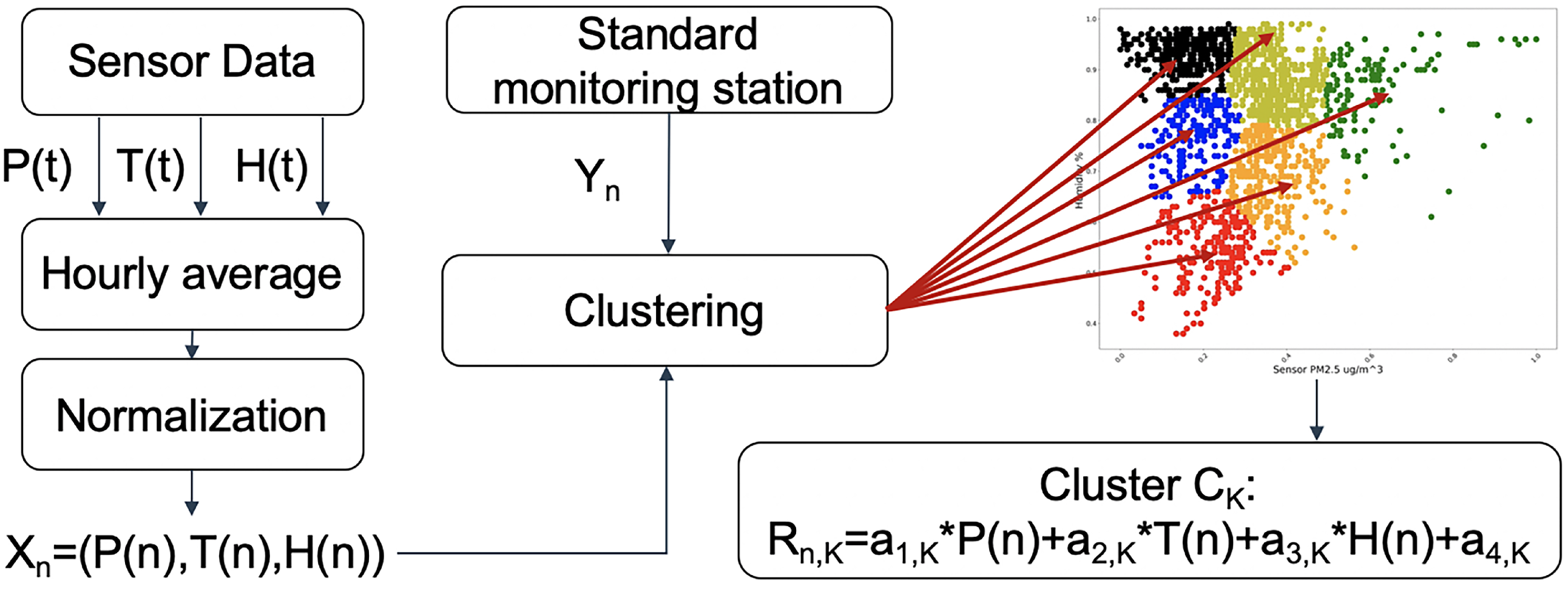
Modeling. Sensory data concerning PM concentration, temperature, and relative humidity are firstly averaged hourly so that they have same interval with PM concentration data from standard monitoring station. Then, normalization of sensory data according to the sensor’s range is required for their range difference. We can combine PM concentration, temperature and relative humidity into tuple X,
where P represents PM concentration, T represents temperature, H represents relative humidity and n is time. Each tuple has an hourly station PM concentration reference corresponding at time n. As shown in Figure 5, with clustering algorithm all samples of are divided into several clusters. For each cluster, a corresponding multiple linear regression model can be calculated with in the cluster,
where are parameters calculated by least square fitting and represent calibrated value of sample in cluster k at time n.
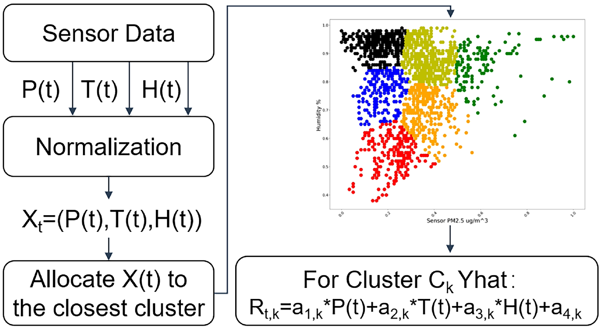
Calibrating. Steps of the calibration stage are shown in Figure 6. With the clusters and their corresponding multiple linear regression models obtained in the modeling step, sensory data of PM concentration can be calibrated. When new samples of sensory data arrive, normalization and combining them into tuple as Equation (1) are preparation steps. Based on the shortest distance under some metric (e.g., Euclidean Distance), tuple can be used to find the cluster it belongs to. If tuple belongs to the cluster k, according to Equation (2), is the calibrated sensory PM concentration at time t and it can be calculated as below:
In practice due to seasonality, the modeling can describe the relationship between deviation and factors (PM concentration, temperature and relative humidity) approximately based on short-term sampled data. Thus, in long-term sensing system deployment, this method needs to be executed periodically and cluster division and corresponding multiple linear regression models require regular updating, in order to catch up with the calibration performance.
3. Results
3.1. Experiment Settings
3.1.1. System and Data
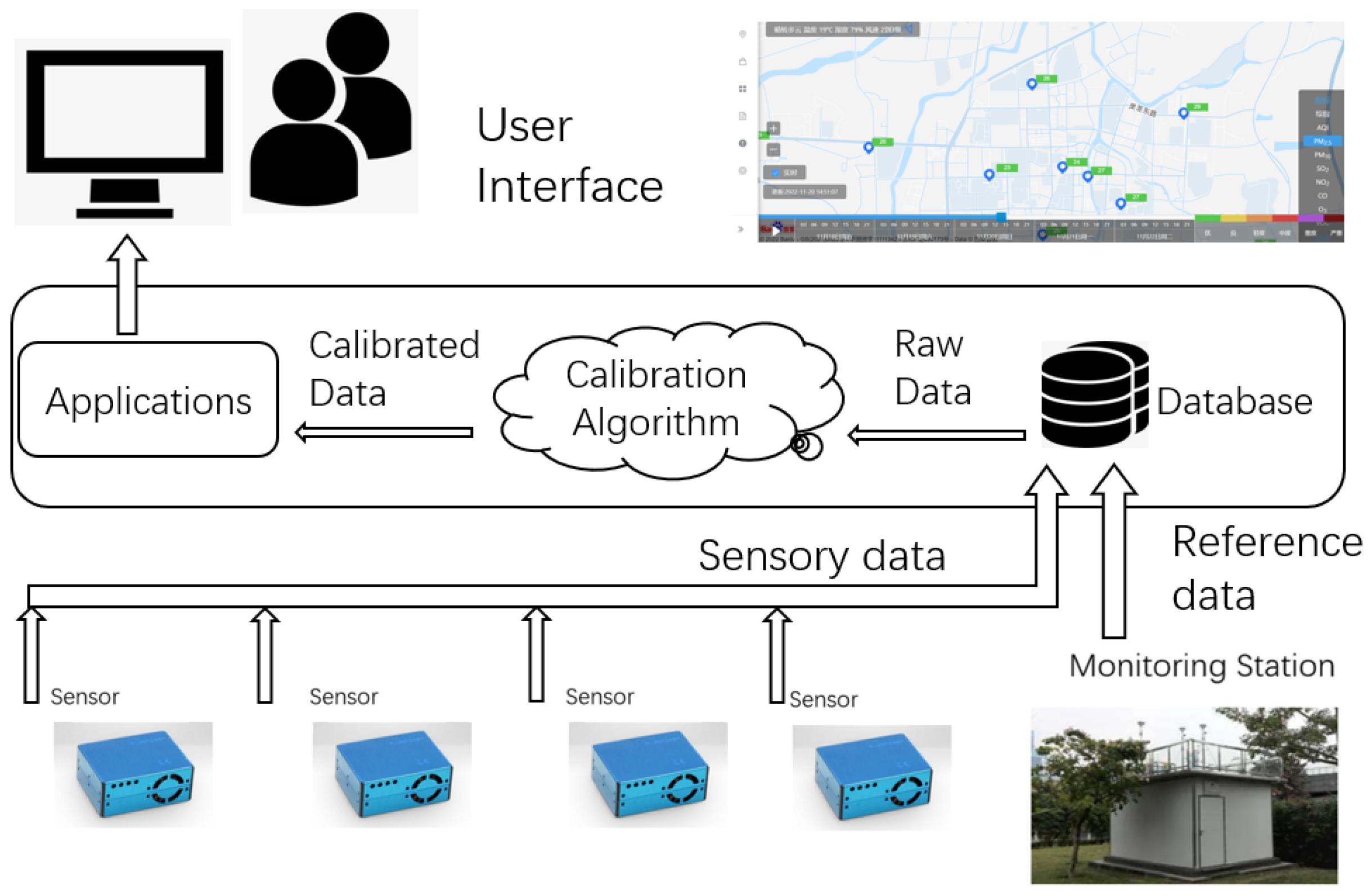
To justify the proposed method, we conduct evaluation with testing data from a practical deployed air pollution sensing system in Anji County, an area near the Taihu Lake, beside Huzhou City in Zhejiang Province as shown in Figure 1. The air pollution sensing system design is shown in Figure 7. Both sensory data and reference data are sampled continuously and saved in the database. Calibration algorithm is implemented on raw in schedule and only calibrated data can be utilized in applications and presented on user interface.
Sensory data are generated by PMS5003S laser particulate matter sensor. It can output PM and PM concentration measurement (g/m) at one-second intervals together with temperature (C) and relative humidity (%). The reference data for calibration are provided at one-hour intervals from official standard atmospheric environment monitoring station, including PM and PM concentration. For in-field calibration testing, the sensor selected is deployed nearby the monitoring station within 30 m range to satisfy the co-location condition.
We prepare three groups of data and each group contains sensory data and reference data in the same three-month period including July–September 2021, October–December 2021 and January–March 2022. To justify the adaptability of the method, the three groups are sampled, respectively, in three different seasons with distinct temperature and humidity conditions, as well as different initial measurement error levels.
When the model calibrates the data set, it first uses the clustering algorithm to cluster the data set, and then divides each cluster into a training set and a test set according to a certain ratio and calculates. The division ratio of the training set is discussed in Section 3.2.5, and it is found that the division ratio of the training set does not have a significant impact on the calibration results.
3.1.2. Evaluation Indicator
In order to evaluate calibration performance, error is defined as the deviation between calibrated sensory data and reference data from station on test set. Root mean square error (RMSE) is selected as the evaluation index. The training set and test set were randomly selected, and the average value of 1000 cycles is used as the benchmark RMSE to measure the impact of various training parameters on the model. The formula is as follows, where is the observation data of the standard station, and is the value of sensor data after model calibration, N represents the number of data in the test set.
3.2. Evaluation
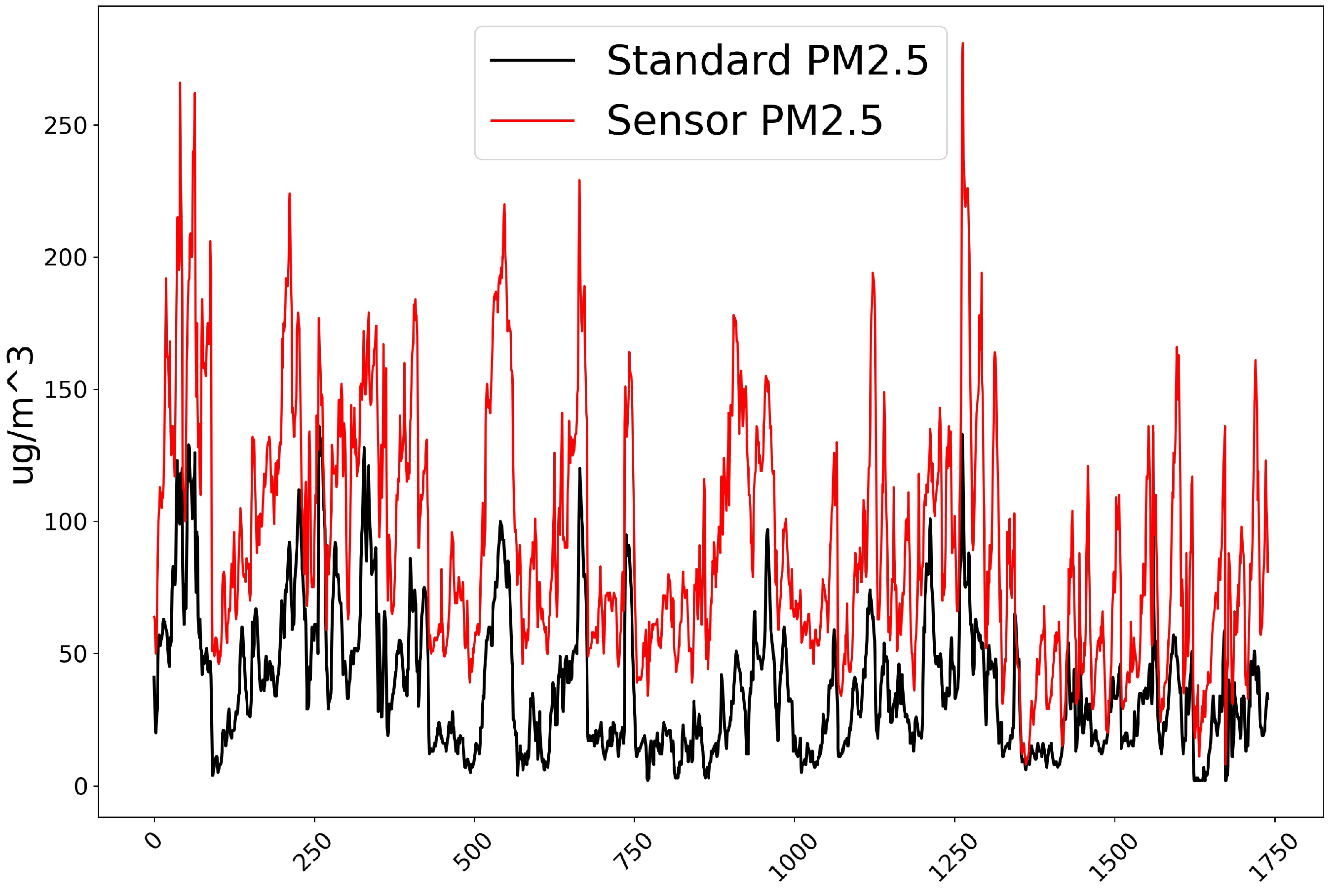
Sensory data of PM concentration are firstly averaged hourly so that they have same interval with PM concentration data from standard monitoring station and compare the sensor data with the standard station. As shown in Figure 8, raw sensory data of PM bear a large initial error compared with standard station in co-location. That is because the sensor has been deployed for a long period of time without adjustment and affected significantly by sensor drift. Other possible causes of the problems are that the environmental conditions will affect the sensor signal, and the sensor is cross sensitive to a variety of pollutants. Raw sensory data of PM have a similar situation.
In our evaluation, a global multiple linear regression model is selected as the baseline comparing with the proposed method. For baseline, we combine constant term, PM concentration, temperature and relative humidity into tuple X, as a parameter of the global multiple linear regression equation. Comparison and analysis involves many aspects.
In Section 3.2.1, we provide a comparison with the original error and baseline proves the effectiveness of our method. In Section 3.2.2, we compare the differences caused by using different algorithms in the clustering stage of the model. In Section 3.2.3, we test the impact of introducing different environment variables on the model clustering and regression stages. Section 3.2.4 presents a comparison concerning the impact of the number of clusters on the calibration results. Section 3.2.5 compares the effects of different proportions of training set test set division on calibration results. In Section 3.2.6, we try to apply the model to the same type of pollutant PM and verify the effect. Section 3.2.7 discusses the stability of the model and the fitting effect on the standard value.
3.2.1. Model Performance Measurement
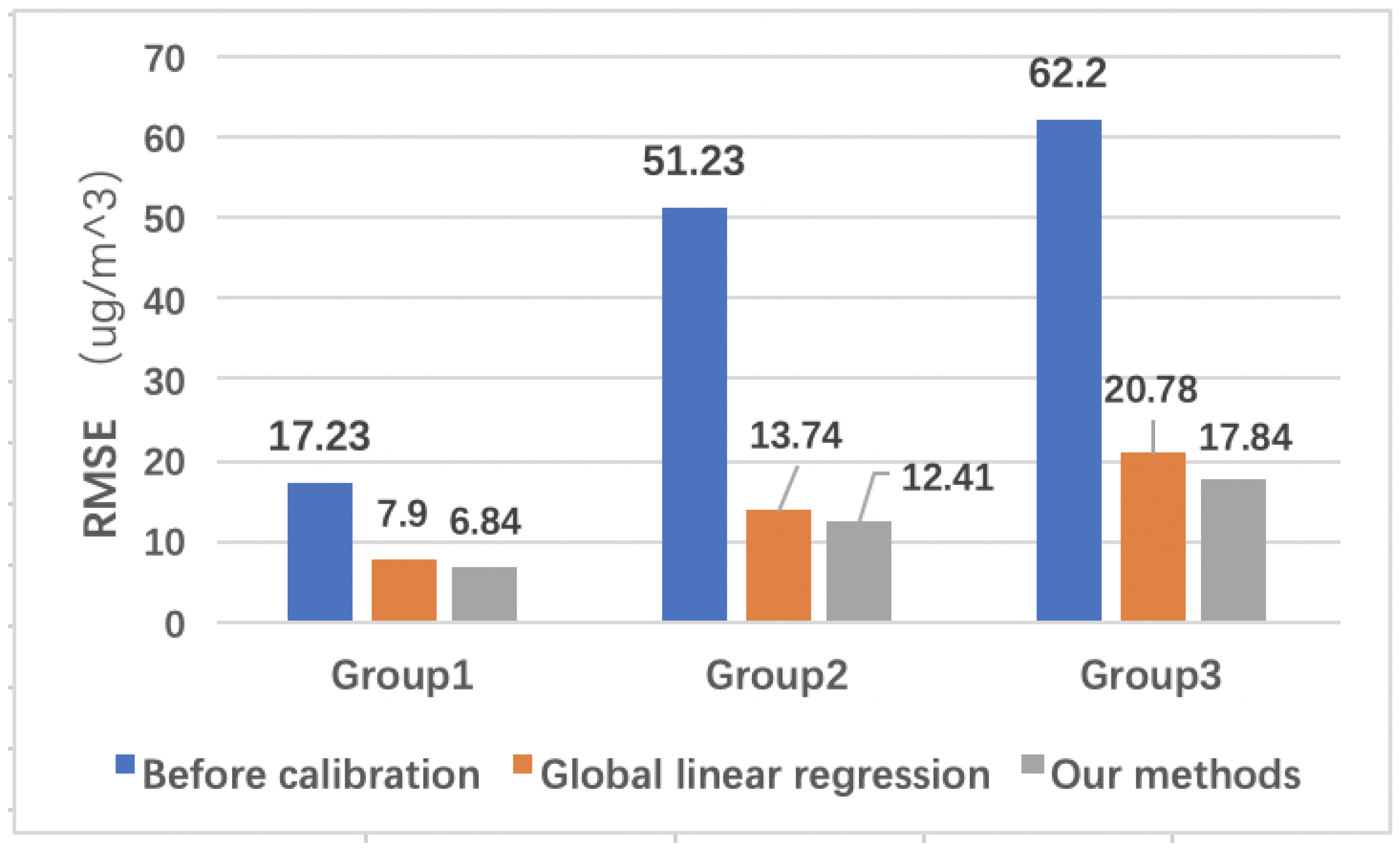
In order to evaluate the performance of the calibration model, we calculate the error between the three groups of sensor PM data and the standard station, respectively. The global linear regression calibration of the sensor PM concentration, relative humidity, and temperature as regression parameters is used as a baseline to measure the performance of our model.
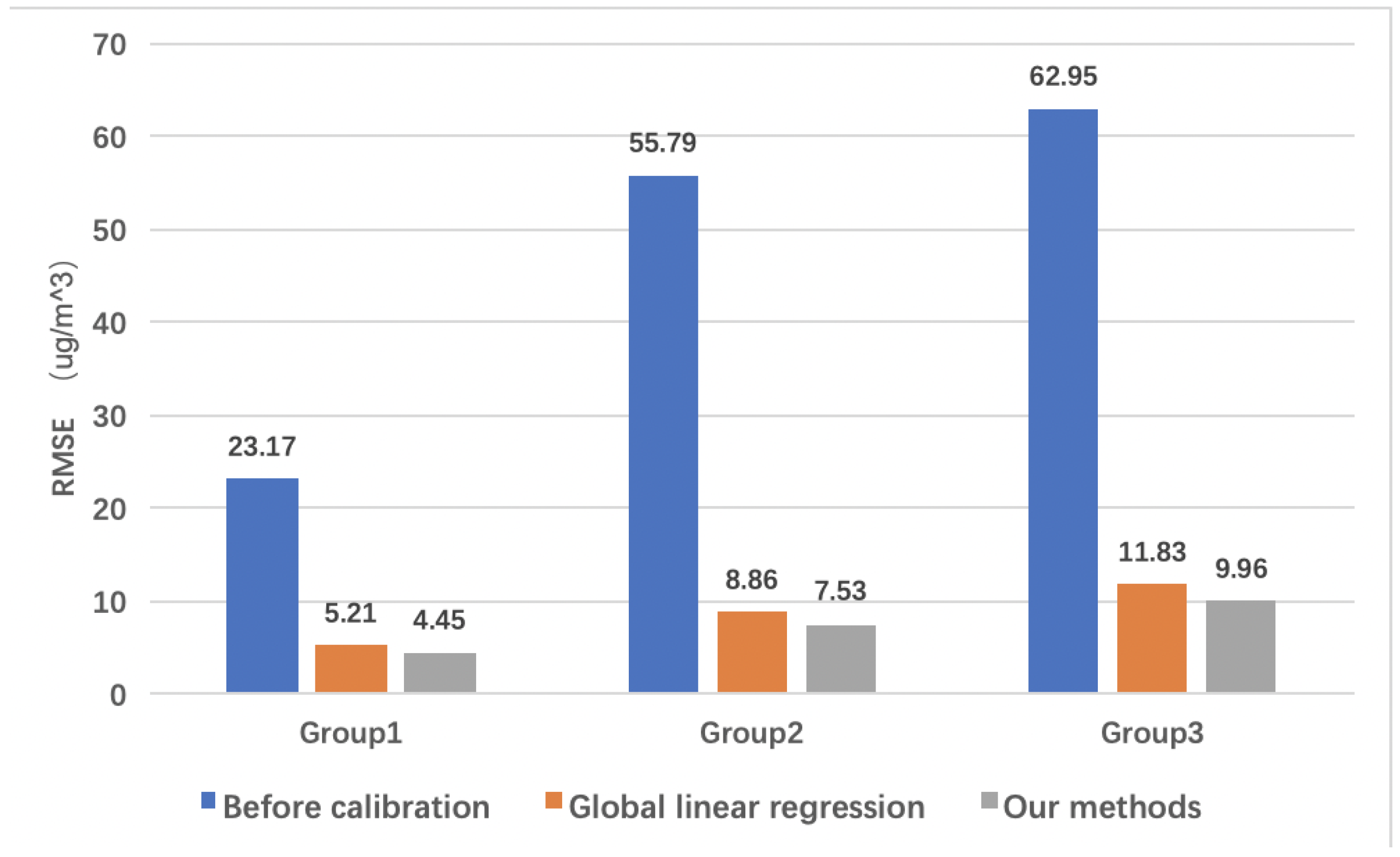
The error between the sensor PM data and the standard station under the global linear regression, is compared with the error between the PM data calibrated by our method and the standard station. As shown in Figure 9, it is found that our method is superior to traditional global regression in three groups of data. The K-means algorithm is used in the data set partition phase of our method. Under K-means, we use as the division basis to divide 6 clusters, and set the ratio of training set and test set to 9:1. For each cluster and global liner regression, we use: as a training parameter of regression model.
3.2.2. Clustering Algorithm
In the clustering phase of the model, selecting different clustering algorithms to partition the data set will have an impact on the effect of subsequent regression training. In order to select an algorithm with low algorithm complexity and good clustering effect and then apply it in the model, the effects of using K-means, Mean-shift [28] and Fuzzy C-means [29,30] as calibration models in the data partitioning phase on the model calibration performance are compared.
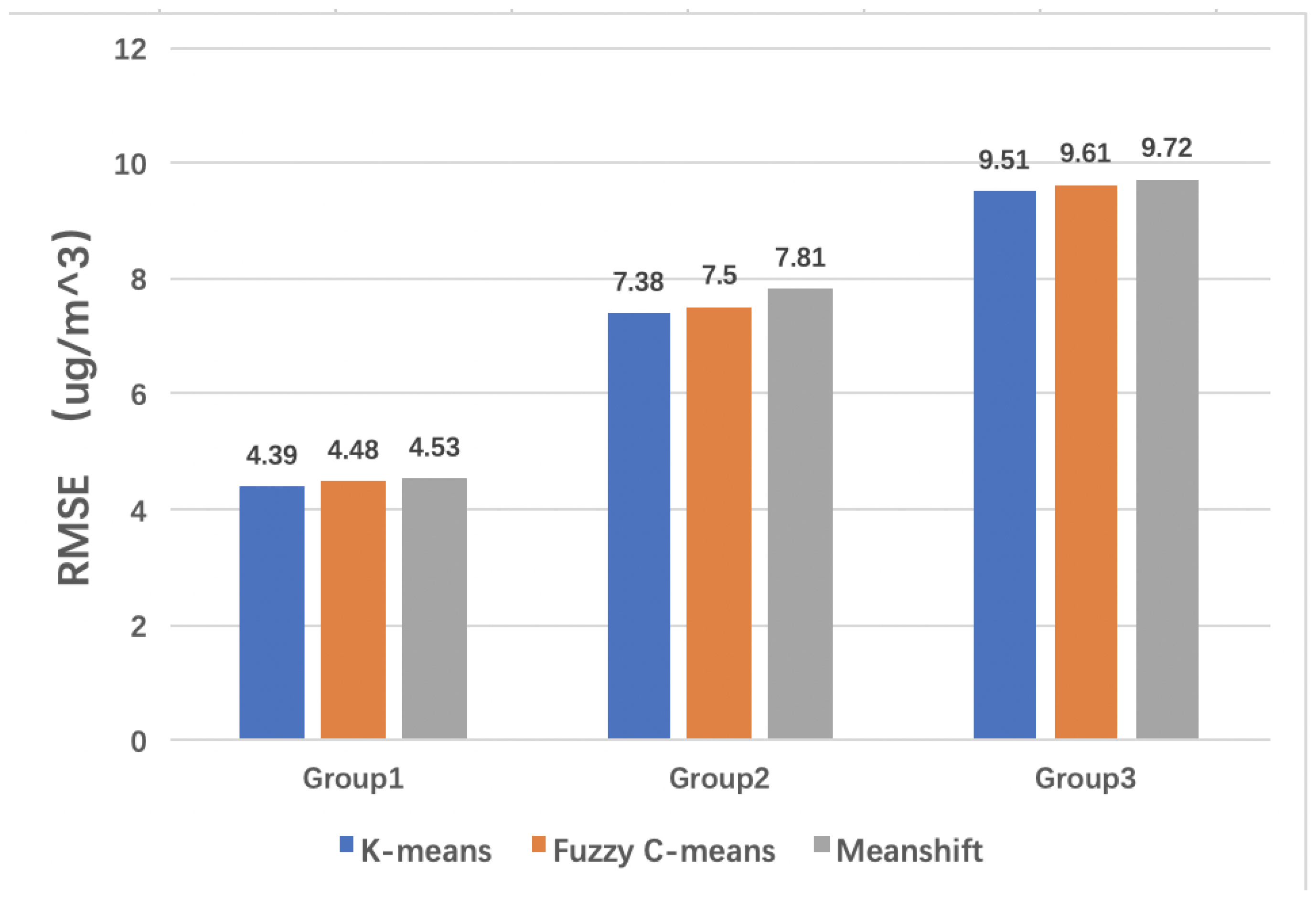
As shown in Figure 10, the RMSE of the three groups of data when using K-means to partition the data set is lower than that of the other two algorithms. Compared with Fuzzy C-means, the RMSE of the three groups of data is reduced by 2%, 1.6%, and 1%, respectively; Compared with Mean-shift, the three groups of data decreased by 3.1%, 5.5% and 2.2% respectively. Among them, Mean-shift is vulnerable to noise interference, and the algorithm is affected by several data points with large offsets. Several similar data points with large offsets are regarded as a cluster, resulting in a small amount of data in the cluster, which cannot be fully trained and will cause large errors. The RMSE of Fuzzy C-means is also slightly higher than that of the K-means, so the subsequent experiments use the K-means algorithm to partition the data set.
3.2.3. Dimension of Clustering
In order to determine the environment variables used in the clustering basis and regression equation, comparative experiments are conducted from two aspects: clustering factor and regression factors. The PM concentration, temperature and humidity data used in clustering are all normalized to ensure that the clustering effect will not be affected by different data ranges.
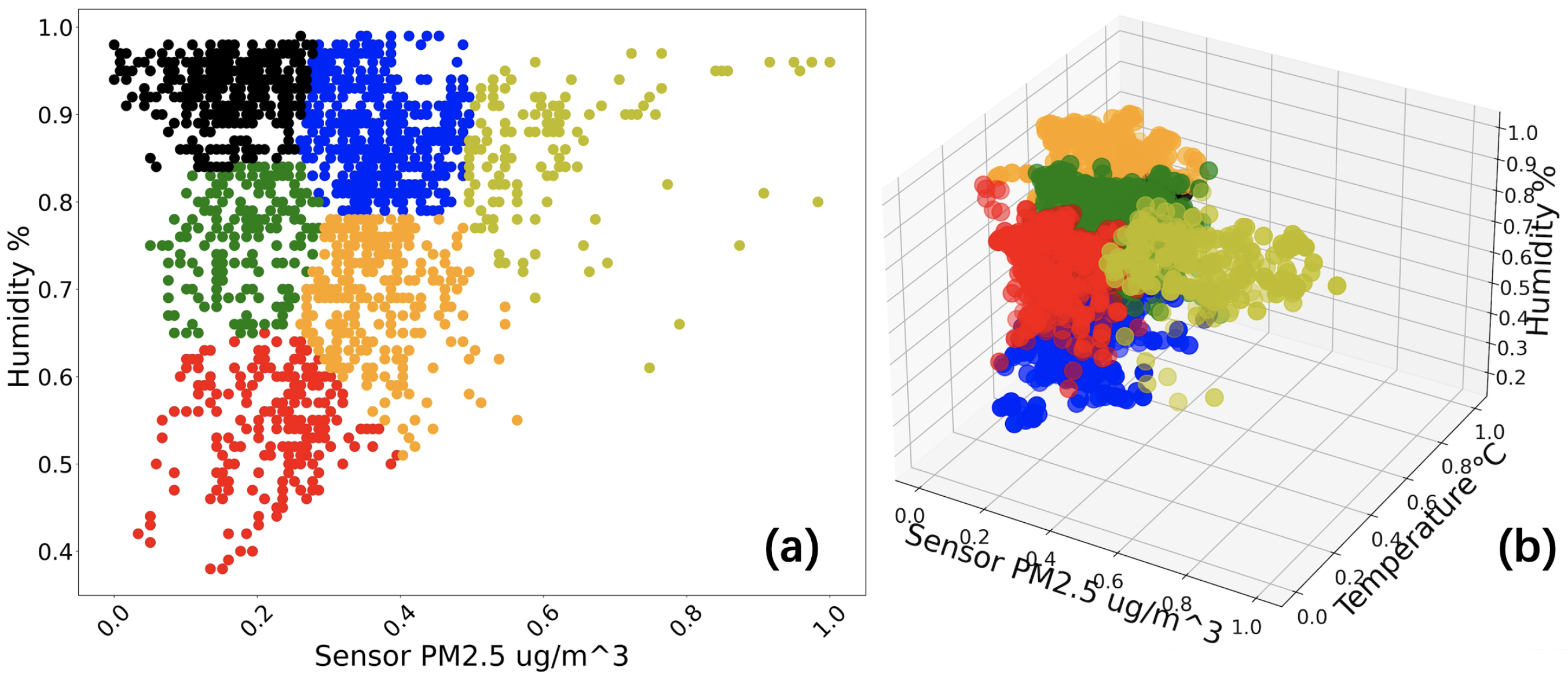
Clustering factors. In order to partition the data set more reasonably and improve the accuracy of the calibration phase, K-means algorithm is used to partition the data set according to different sensor information. Three different dimensions of clustering tests were conducted. The Figure 11 shows the intuitive effect of data samples clustering under two-dimensional and three-dimensional case.
As shown in Table 1, in the Group 1 data group, regression the divided data set to obtain calibration parameters, and calculate the PM concentration after calibration on the test set, after calibration, the RMSE values of the three different division methods and the standard data are 4.63, 4.48 and 4.46, respectively. Compared with the clustering based on concentration and temperature, two-dimensional clustering with concentration and humidity, and three-dimensional clustering with both concentration and temperature and humidity were used. RMSE after regression decreased by 3.24% and 3.67%, which also had the same effect on Group 2 and Group 3. RMSE in Group 2 decreased by 21.82%, 20.58%, and that in Group 3 decreased by 14.39%, 15.62%. It can be seen that whether it is two-dimensional or three-dimensional clustering, introducing humidity as one of the classification criteria can significantly improve calibration performance.
Regression factors. In order to further compare the effects of humidity and temperature on the calibration performance of the sensor, humidity is introduced into the regression equation in the two-dimensional division based on concentration temperature clustering. It is found that the RMSE in the three groups of data decreased by 3.89%, 22.13% and 12.09%, respectively, compared with those before the introduction, and all obtained objective improvement. Then, by comparing the concentration temperature humidity ternary as the training parameter of the regression equation, it is determined that when the concentration humidity is used as the clustering basis and the concentration, temperature and humidity are used as the regression parameters, compared with baseline, the RMSE of the three groups of data after calibration decreased by 16.89%, 17.27% and 20.37%, respectively, the best calibration performance can be achieved in the three groups of data under the existing conditions.
Based on the above experiments, the PM concentration, humidity are used as the classification basis in the three groups of data, and the PM concentration, temperature, humidity are used as the training parameters in the regression equation to obtain the best effect. Compared with the three-dimensional K-means clustering, it can also have lower overhead. Therefore, we suggest using the two-dimensional K-means clustering method combined with the multiple linear regression equation.
3.2.4. Number of Clusters
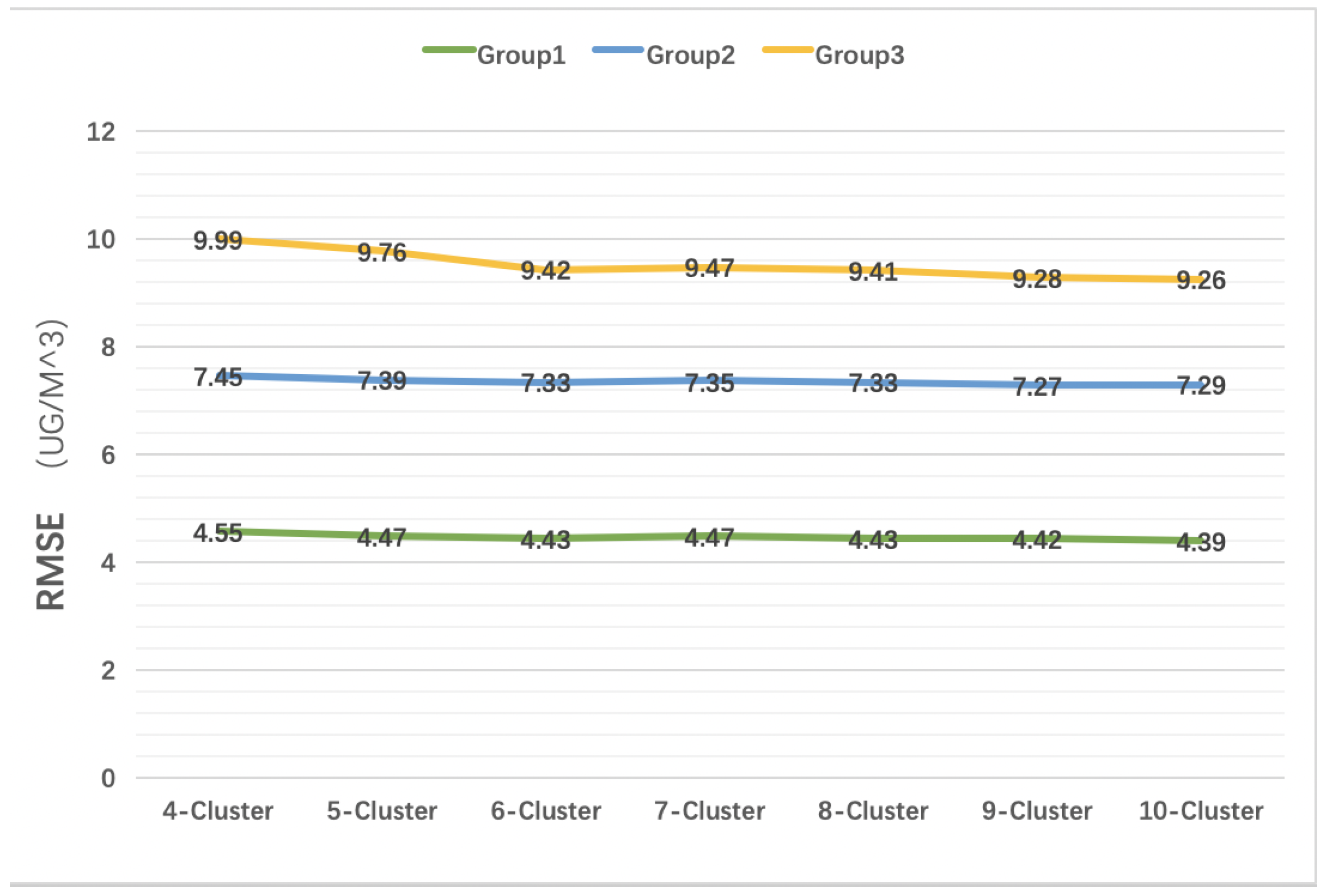
After selecting the clustering factors and regional factors in the previous section, we test the impact of the number of clusters on the calibration performance. As shown in Figure 12, it is found that the RMSE of the three groups of data decreases with an increase of the number of K-means clusters. However, when the number of clusters increases to a certain range, the reduction of RMSE is limited.
Therefore, we can choose a moderate number of clusters, such as 6, as this can control the amount of computation in a small range to obtain sufficient calibration performance.
3.2.5. Training Set and Testing Set Division
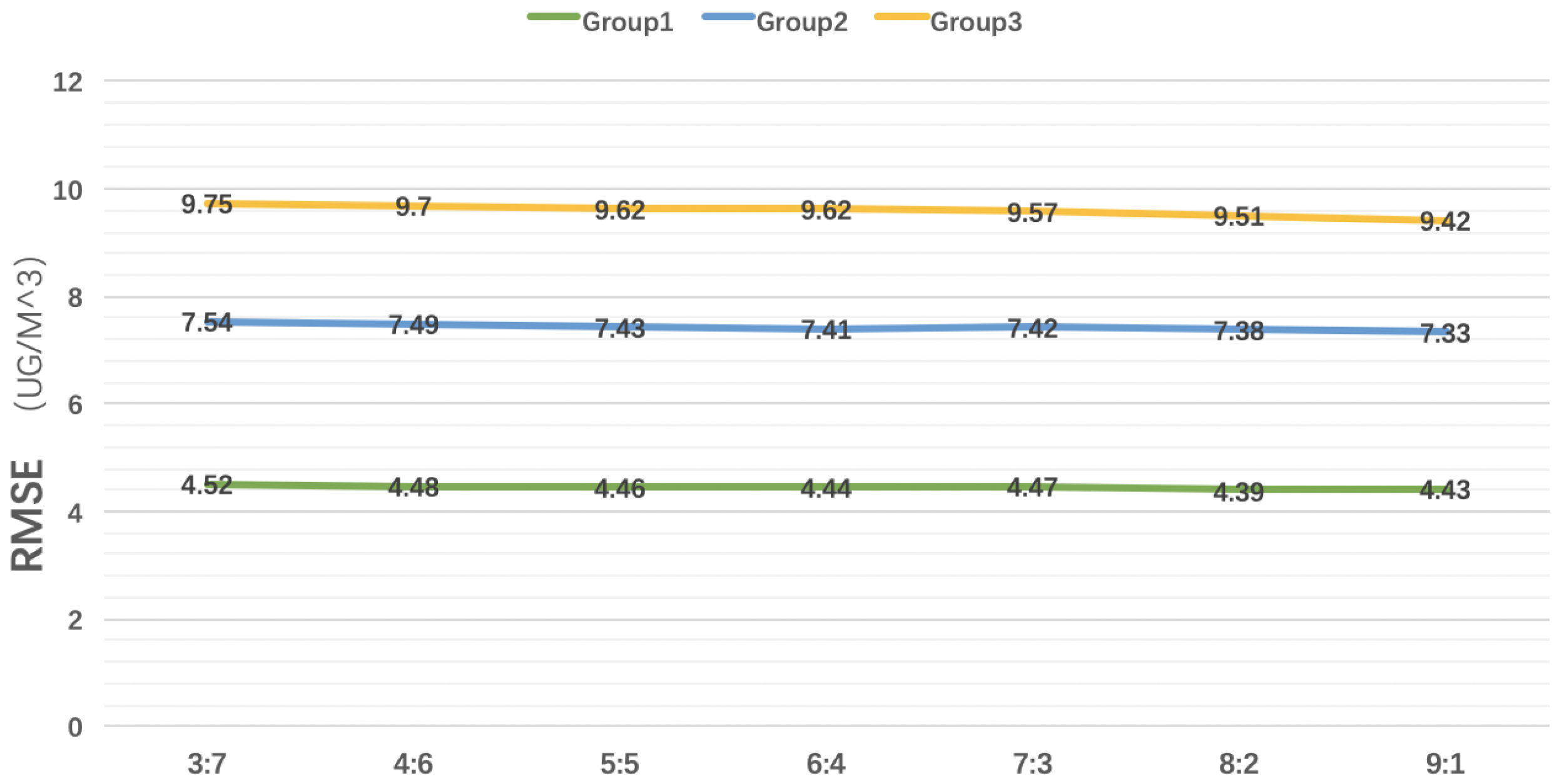
In order to evaluate the influence of different division ratios of training sets and test sets on the calibration model, we compare the division methods from 3:7 to 9:1 in three groups of data, with gradually increased the proportion of training sets. As shown in Figure 13, it can be seen that RMSE decreases with the increase of training set partition proportion, but the impact on RMSE decreases marginally with the increase of training set partition.
Therefore, we prefer to use a smaller proportion of training sets to achieve the effect not inferior to the high proportion of training set partition. In this way, we cannot only obtain more test sets to verify the effect of model training, but also avoid the problem of overfitting.
3.2.6. Performance on PM
In order to test the calibration effect of our model on the same type of pollutants, the model is used on the PM concentration data. Similarly, after the data is normalized, the model is divided according to the PM concentration, humidity, and then the PM concentration, temperature, humidity are trained as regression parameters. The calibration results are shown in Figure 14, the PM concentration measured by the sensor has a large initial error before calibration. After calibration by our method, the RMSE of the three groups of data is 13.42%, 9.68%, 14.15% lower than that of the global linear regression calibration. These results show that our method is effective for calibrating data from similar sensors.
Comparing the performance of our method applied to the calibration of PM and PM pollutants, we can see that there is a good improvement in the data of three groups of different periods. As shown in Table 2, our method is available for calibrating both PM and PM sensory data.
3.2.7. Stability of the Model
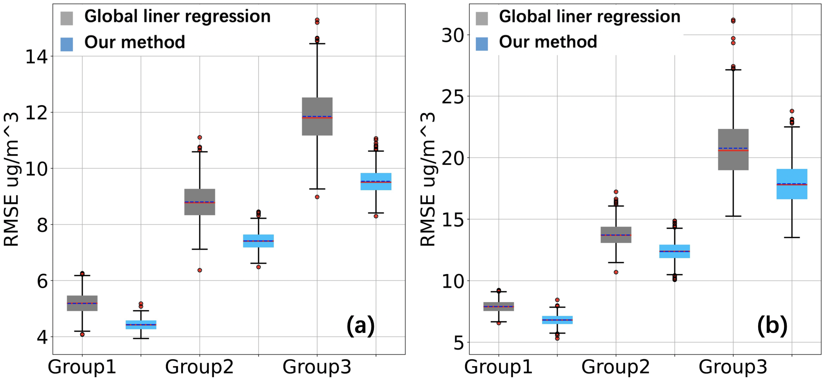
The training set of model calibration segment is randomly selected from the data set according to a certain proportion. In order to measure the stability of our method, we test whether the calibration effect will fluctuate greatly due to the change of training set selection. We record the RMSE between calibration value and standard station data due to different training set selections when using global linear regression to calibrate PM data and PM data of sensors on the same set of data for many times, and the RMSE caused by different training set selections when using our method to calibrate PM data and PM data of sensors. The RMSE data in the two groups of tests are formed into a boxplot. As shown in Figure 15, when applied to PM and PM pollutants, our method has lower error than the global linear regression in addition to lower variance, and improvements in stability of calibration performance are achieved.
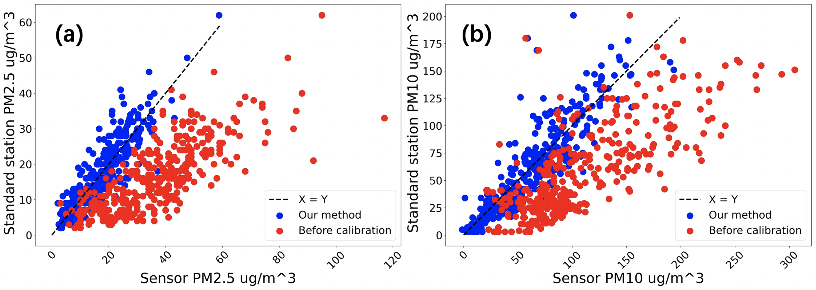
We take the target pollutant concentration of the sensor as the X-axis, and the target pollutant concentration provided by the standard station as the Y-axis. The data before the calibration of the sensor PM are displayed with red scatter points, the sensor PM data calibrated with our method are displayed with blue scatter points, and the data of PM are also plotted with the same method. In an ideal case, the data measured by the sensor should be equal to the reference value provided by the standard station. The scatter diagram in this coordinate system is in the shape of X = Y. However as shown in Figure 16, due to the influence of sensor performance and environment, the data before PM and PM calibration contains a large error, that is far from X = Y. After our method calibration, the data error is reduced, and the distribution is pulled back to the X = Y axis, which is extremely effective in the application of PM and PM pollutants.
In order to measure the fitting degree between the sensor concentration data processed by the model and the data of the standard station, the determination coefficient is used as an indicator. Compared with the baseline before calibration, our method is used for calibration. As shown in Table 3, in these three cases, the of the sensor PM and PM concentration and the standard station PM and PM concentration can be seen that the sensor target pollutant concentration calibrated by our method has a higher fitting degree to the standard station and is closer to the true value.
4. Discussion
Theoretically, in this regression calibration problem, the proposed method divides the whole independent variable space into several parts and allocates one multiple linear regression model for each part. It does not rely on prior knowledge of sensor characteristics but is determined by practical sensory data sampling. This method uses a combination of linear regression models to approximate a complex function structure, relieving the underfitting problem caused by a rough global multiple linear regression model. Inspired by this, the sensor’s cross-sensitivity calibration problem can also apply the proposed method to divide its independent variable space with more dimensions and simplify calibration model expression. Compared with a complex global regression model or ANN-based learning model, the proposed method makes the calibration model much easier to determine and explain.
In evaluation, we find that when factor relative humidity is involved in clustering or regression, the performance improves more obviously than factor temperature. That is because humidity has an influence in the mechanism of sensor response. The output signals of laser particulate matter sensor depend on laser scattering caused by particulate matter in the sensor responding chamber. Thus, when environment humidity is high or increases sharply over a short period, numerous ambient floating micro-liquid drops will form in the chamber together with particulate matter, affecting laser scattering and the sensor’s response. This process is hard to model physically; however, data-driven methods can describe the influence of humidity without knowing chamber structure design, laser scattering or other hardware issues.
In total, three groups of data crossing different seasons including summer–autumn (Group 1), autumn–winter (Group 2) and winter–spring (Group 3) are involved in evaluation. Data in winter and spring achieved a larger calibration error than those in autumn. That is because for the location our system was deployed, there are more particulate-matter-related weather events or pollution events happening during the period of autumn to spring the next year. Within such pollution processes, the particulate matter concentration in atmosphere environment is greater. According to Figure 2 and Figure 16, there are more difficulties to reducing calibration error. Calibration error and coefficient of determination regarding PM are slightly better than that on PM. Generally, PM has higher concentration and wider dynamic range than PM on the sensor’s readings. This may lead to larger calibration error mean value and error variance concerning PM readings. In addition, PM is affected more by humidity than PM in PM sensor measurements. When laser scattering is affected by numerous liquid drops, there will be a larger PM measurement deviation, which was observed in practice. This suggests that the in-field calibration model for PM may be more sophisticated than that for PM.
Better of the proposed method than the global linear regression model might be attributed to clustering. The whole independent variable space is divided by clustering and each cluster possesses a number of samples. If each cluster has sufficient and typical enough samples, it can reach a good fitting degree. However on the other hand, clustering may also lead to some disadvantages in using our method. One such disadvantage is extremely unbalanced sizes of clusters. A cluster with few samples cannot obtain a satisfying regression model and will lead to a large error variance. Outliers and incorrect classification will also bring negative influence on calibration performance. These are issues worth further discussion.
5. Conclusions
In general, we design a method using a clustering algorithm to realize segmented regression for in-field sensor calibration. It can compensate for humidity and temperature interference on PM sensor with statistical characteristics of samples and less prior knowledge, using a combination of linear regression models. Samples for modeling are divided into clusters via clustering algorithm and each cluster has its own individual multiple linear regression model calculated from least square fitting. The final calibrated result of one sensory sample is calculated from the regression model of the cluster the sample itself belongs to. Theoretically, the proposed method divides the whole independent variable space into several parts and allocates one multiple linear regression model for each part. This provides a more meticulous function for sensory data calibration and to some extent, can overcome the underfitting problem of using a global multiple linear regression model.
The proposed method is evaluated on a practical deployed air pollution sensing system using official monitoring station as calibration reference, and a global multiple linear regression model as the baseline. An evaluation on the data set of different initial error levels indicates that the clustering-based calibration method produces a better performance. It works on the sensory data of both PM and PM, and provides at least 16% and 9% improvement ratio of calibration error on RMSE, respectively, for pollutants PM and PM compared with the baseline. Regarding error statistics, the error of our method has both a smaller mean value and variance than the global linear regression model meaning that our method produces superior stability among numerous random tests. Besides both on PM and PM, our method has a better fitting degree due to a better determination coefficient than the baseline.
Our experiments consider different combinations of clustering factors and regression factors. It is found that under existing conditions the best calibration effect is achieved when clustering factors include PM concentration and humidity, and regression factors include PM concentration, humidity and temperature. Relative humidity has an appreciable influence and corresponds with usage experience and mechanism of the laser particulate matter sensor.
The evaluation also shows that the proposed method may have a lower calculation cost. Because the calibration error is not quite sensitive to cluster number and the ratio of training set and testing set, this means that a moderate number of clusters is sufficient, and the training data can be reduced to relieve over-fitting problem. These benefits can improve the efficiency of post-deployment sensor calibration.
Furthermore, there are several aspects for future research regarding the proposed method. In practical sensor deployment, calibration model updating warrants further attention because the proposed method has seasonal limitation based on limited sampling. The updating involves clustering updating and regression parameters updating, both on accuracy and efficiency. Optimization on clustering algorithms is another attractive issue and the selection of clustering algorithms may be related to multiple-dimension sensory data distribution. In addition, the existing evaluation only involves the current status of variables and does not consider delay items of the variables. If reflecting the changing process of some environmental factors in the model, e.g., humidity, it can improve calibration performance, delay items such as , and require to be added in regression models. Last but not least, since the method works on PM and PM calibration against temperature and humidity, it also has potential value in assisting the sensor’s cross-sensitivity calibration problem and may be more efficient than pre-deployment laboratory calibration.
Author Contributions
Conceptualization, S.L. and X.L.; methodology, S.L. and X.L.; software, S.L.; validation, S.L. and X.L.; formal analysis, S.L.; investigation, S.L.; resources, X.L.; writing—original draft preparation, S.L.; writing—review and editing, S.L. and X.L.; supervision, P.L.; project administration, P.L.; funding acquisition, P.L. All authors have read and agreed to the published version of the manuscript.
Funding
This research was funded by the National Key Research and Development Program of China (No. 2020AAA0105802), the National Natural Science Foundation of China (No. 62066011, 61906192), the Natural Science Foundation of Guangxi Zhuang Autonomous Region (No. 2022GXNSFAA035640), and the PhD Research Startup Foundation of Guilin University of Technology (No. GUTQDJJ2019175, GUTQDJJ2019176).
Institutional Review Board Statement
Not applicable.
Informed Consent Statement
Not applicable.
Data Availability Statement
Not applicable.
Acknowledgments
We thank Shenzhen Environmental Thinking Science and Technology (ETST) Co., Ltd. for their assistance in sensor deployment and data sampling.
Conflicts of Interest
The authors declare no conflict of interest.
References
- De Jesus, A.L.; Thompson, H.; Knibbs, L.D.; Kowalski, M.; Cyrys, J.; Niemi, J.V.; Kousa, A.; Timonen, H.; Luoma, K.; Petaja, T.; et al. Long-term trends in PM2.5 mass and particle number concentrations in urban air: The impacts of mitigation measures and extreme events due to changing climates. Environ. Pollut. 2020, 263, 114500. [Google Scholar] [CrossRef] [PubMed]
- Mead, M.I.; Popoola, O.; Stewart, G.B.; Landshoff, P.; Calleja, M.; Hayes, M.; Baldovi, J.J.; Mcleod, M.W.; Hodgson, T.F.; Dicks, J.; et al. The use of electrochemical sensors for monitoring urban air quality in low-cost, high-density networks. Atmos. Environ. 2013, 70, 186–203. [Google Scholar] [CrossRef] [Green Version]
- Delaine, F.; Lebental, B.; Rivano, H. In Situ Calibration Algorithms for Environmental Sensor Networks: A Review. IEEE Sens. J. 2019, 19, 5968–5978. [Google Scholar] [CrossRef] [Green Version]
- Tsujita, W.; Yoshino, A.; Ishida, H.; Moriizumi, T. Gas sensor network for air-pollution monitoring. Sens. Actuators B Chem. 2005, 110, 304–311. [Google Scholar] [CrossRef]
- Kumar, P.; Morawska, L.; Martani, C.; Biskos, G.; Neophytou, M.; Sabatino, S.D.; Bell, M.; Norford, L.; Britter, R. The rise of low-cost sensing for managing air pollution in cities. Environ. Int. 2015, 75, 199–205. [Google Scholar] [CrossRef] [Green Version]
- Velasco, A.; Ferrero, R.; Gandino, F.; Montrucchio, B.; Rebaudengo, M. A Mobile and Low-Cost System for Environmental Monitoring: A Case Study. Sensors 2016, 16, 710. [Google Scholar] [CrossRef] [PubMed]
- Chen, X.; Xu, S.; Fu, H.; Joe-Wong, C.; Zhang, L.; Noh, H.Y.; Zhang, P. ASC: Actuation system for city-wide crowdsensing with ride-sharing vehicular platform. In Proceedings of the Fourth Workshop on International Science of Smart City Operations and Platforms Engineering, Montreal, QC, Canada, April 2019; pp. 19–24. [Google Scholar] [CrossRef]
- Devarakonda, S.; Sevusu, P.; Liu, H.; Liu, R.; Iftode, L.; Nath, B. Real-time air quality monitoring through mobile sensing in metropolitan areas. In Proceedings of the ACM SIGKDD International Workshop on Urban Computing, Chicago, IL, USA, 11 August 2013. [Google Scholar]
- Xu, S.; Chen, X.; Pi, X.; Joe-Wong, C.; Zhang, P.; Noh, H.Y. iLOCuS: Incentivizing Vehicle Mobility to Optimize Sensing Distribution in Crowd Sensing. IEEE Trans. Mob. Comput. 2020, 19, 1831–1847. [Google Scholar] [CrossRef]
- Sun, L.; Westerdahl, D.; Zhi, N. Development and Evaluation of A Novel and Cost-Effective Approach for Low-Cost NO2 Sensor Drift Correction. Sensors 2017, 17, 1916. [Google Scholar] [CrossRef] [PubMed]
- Nicholas, M.; Ricardo, P.; Michael, H. Quantification Method for Electrolytic Sensors in Long-Term Monitoring of Ambient Air Quality. Sensors 2015, 15, 27283–27302. [Google Scholar]
- Cross, E.S.; Williams, L.R.; Magoon, G.R.; Onasch, T.B.; Kaminsky, M.L.; Worsnop, D.R.; Jayne, J.T. Use of electrochemical sensors for measurement of air pollution: Correcting interference response and validating measurements. Atmos. Meas. Tech. 2017, 10, 3575–3588. [Google Scholar] [CrossRef]
- Day, D.E.; Malm, W.C. Aerosol light scattering measurements as a function of relative humidity: A comparison between measurements made at three different sites. Atmos. Environ. 2001, 35, 5169–5176. [Google Scholar] [CrossRef]
- Padilla, M.; Perera, A.; Montoliu, I.; Chaudry, A.; Persaud, K.; Marco, S. Drift compensation of gas sensor array data by orthogonal signal correction. Chemom. Intell. Lab. Syst. 2010, 100, 28–35. [Google Scholar] [CrossRef]
- Chen, H.X. Research on multi-sensor data fusion technology based on BP neural network. In Proceedings of the 2015 International Workshop on Wireless Communication and Network (IWWCN2015), Kunming, China, 21–23 August 2015. [Google Scholar]
- Maag, B.; Zhou, Z.; Thiele, L. A Survey on Sensor Calibration in Air Pollution Monitoring Deployments. IEEE Internet Things J. 2018, 5, 4857–4870. [Google Scholar] [CrossRef] [Green Version]
- Li, G.; Wu, Z.; Liu, N.; Liu, X.; Wang, Y.; Zhang, L. A Variational Bayesian Blind Calibration Approach for Air Quality Sensor Deployments. IEEE Sens. J. 2022. [Google Scholar] [CrossRef]
- Li, G.; Ma, R.; Liu, X.; Wang, Y.; Zhang, L. RCH: Robust calibration based on historical data for low-cost air quality sensor deployments. In Proceedings of the Adjunct Proceedings of the 2020 ACM International Joint Conference on Pervasive and Ubiquitous Computing and Proceedings of the 2020 ACM International Symposium on Wearable Computers, Virtual Event, Mexico, 12–17 September 2020; pp. 650–656. [Google Scholar]
- Maag, B.; Saukh, O.; Hasenfratz, D.; Thiele, L. Pre-Deployment Testing, Augmentation and Calibration of Cross-Sensitive Sensors. In Proceedings of the EWSN 2016, Graz, Austria, 15–17 February 2016. [Google Scholar]
- Mijling, B.; Jiang, Q.; de Jonge, D.; Bocconi, S. Field calibration of electrochemical NO2 sensors in a citizen science context. Atmos. Meas. Tech. 2018, 11, 1297–1312. [Google Scholar] [CrossRef] [Green Version]
- Vergara, A.; Vembu, S.; Ayhan, T.; Ryan, M.A.; Homer, M.L.; Huerta, R. Chemical gas sensor drift compensation using classifier ensembles. Sens. Actuators 2012, B166–167, 320–329. [Google Scholar] [CrossRef]
- Patra, J.C.; Ang, E.L.; Meher, P.K. A novel neural network-based linearization and auto-compensation technique for sensors. In Proceedings of the IEEE International Symposium on Circuits & Systems, Kos, Greece, 21–24 May 2006. [Google Scholar]
- Topalovic, D.B.; Davidovic, M.; Jovanovic, M.; Bartonova, A.; Ristovski, Z.; Jovasevic-Stojanovic, M. In search of an optimal in-field calibration method of low-cost gas sensors for ambient air pollutants: Comparison of linear, multilinear and artificial neural network approaches. Atmos. Environ. 2019, 213, 640–658. [Google Scholar] [CrossRef]
- Mueller, M.; Meyer, J.; Hueglin, C. Design of an ozone and nitrogen dioxide sensor unit and its long-term operation within a sensor network in the city of Zurich. Atmos. Meas. Tech. 2017, 10, 3783–3799. [Google Scholar] [CrossRef] [Green Version]
- Yamamoto, K.; Togami, T.; Yamaguchi, N.; Ninomiya, S. Machine learning-based calibration of low-cost air temperature sensors using environmental data. Sensors 2017, 17, 1290. [Google Scholar] [CrossRef] [Green Version]
- Lin, Y.; Dong, W.; Chen, Y. Calibrating low-cost sensors by a two-phase learning approach for urban air quality measurement. Proc. ACM Interact. Mob. Wearable Ubiquitous Technol. 2018, 2, 1–18. [Google Scholar] [CrossRef]
- Murugesan, K.; Zhang, J. Hybrid bisect K-means clustering algorithm. In Proceedings of the IEEE 2011 International Conference on Business Computing and Global Informatization, Shanghai, China, 29–31 July 2011; pp. 216–219. [Google Scholar]
- Barash, D.; Comaniciu, D. Meanshift clustering for DNA microarray analysis. In Proceedings of the Computational Systems Bioinformatics Conference, 2004. CSB 2004, Stanford, CA, USA, 19 August 2004. [Google Scholar]
- Chuang, K.S.; Tzeng, S.; Chen, J.W.; Chen, T. Fuzzy c-means clustering with spatial information for image segmentation. Comput. Med. Imaging Graph. 2006, 30, 9–15. [Google Scholar] [CrossRef] [PubMed] [Green Version]
- Zhao, F.; Jiao, L.; Liu, H. Kernel generalized fuzzy c-means clustering with spatial information for image segmentation. Digit. Signal Process. 2013, 23, 184–199. [Google Scholar] [CrossRef]
Figure 1.
In-field calibration is conducted when the sensor is in close proximity to the station. The station data can be regarded as ground truth and a regression model is to be obtained from sensor data to ground truth. The system for our research is deployed in Anji County, near Huzhou City in Zhejiang Province.

Figure 2.
Samples: Sensory PM concentration vs. error to be calibrated.

Figure 3.
Samples: Sensory relative humidity vs. error to be calibrated (PM).

Figure 4.
Samples: Sensory temperature vs. error to be calibrated (PM).

Figure 5.
Modeling stage: Clustering-based segmented regression.

Figure 6.
Calibrating stage: Clustering-based segmented regression.

Figure 7.
In the system design, raw data are calibrated via the calibration algorithm based on sensory data and reference data are sampled and then utilized in various applications.
Figure 7.
In the system design, raw data are calibrated via the calibration algorithm based on sensory data and reference data are sampled and then utilized in various applications.

Figure 8.
Sensor PM(red line) and in-field standard stations PM(black line), data comparison three-months post-deployment.
Figure 8.
Sensor PM(red line) and in-field standard stations PM(black line), data comparison three-months post-deployment.

Figure 9.
Taking RMSE as the evaluation index, the initial error of PM concentration between the sensor and the standard station, the error after global linear regression and the error processed by our method are calculated.
Figure 9.
Taking RMSE as the evaluation index, the initial error of PM concentration between the sensor and the standard station, the error after global linear regression and the error processed by our method are calculated.

Figure 10.
Taking RMSE as the evaluation index, the calibration performance of the model is compared when K-means, Fuzzy c-means, and Mean-shift algorithms are used to partition data sets.
Figure 10.
Taking RMSE as the evaluation index, the calibration performance of the model is compared when K-means, Fuzzy c-means, and Mean-shift algorithms are used to partition data sets.

Figure 11.
The normalized PM concentration, temperature and humidity are used as the clustering basis for K-means. As (a) shows the result of six clusters based on PM concentration and humidity, as (b) is the result of six clusters based on PM concentration, temperature and humidity.
Figure 11.
The normalized PM concentration, temperature and humidity are used as the clustering basis for K-means. As (a) shows the result of six clusters based on PM concentration and humidity, as (b) is the result of six clusters based on PM concentration, temperature and humidity.

Figure 12.
We use RMSE as an indicator to evaluate under the condition of determining the basis for clustering of K-means and the training parameters of regression equation, the effect of selecting different number of K-means clustering on the performance of calibration model.
Figure 12.
We use RMSE as an indicator to evaluate under the condition of determining the basis for clustering of K-means and the training parameters of regression equation, the effect of selecting different number of K-means clustering on the performance of calibration model.

Figure 13.
Taking RMSE as the evaluation index, we compare the influence of different training set division ratios on the calibration results from 3:7 to 9:1 under the given clustering mode and regression parameters of K-means.
Figure 13.
Taking RMSE as the evaluation index, we compare the influence of different training set division ratios on the calibration results from 3:7 to 9:1 under the given clustering mode and regression parameters of K-means.

Figure 14.
Taking RMSE as the evaluation index, the initial error of PM concentration between the sensor and the standard station, the error after global linear regression and the error processed by our method are calculated.
Figure 14.
Taking RMSE as the evaluation index, the initial error of PM concentration between the sensor and the standard station, the error after global linear regression and the error processed by our method are calculated.

Figure 15.
PM (a) and PM (b) are taken as the target calibration values, the global linear regression and our method are tested repeatedly numerous times, respectively. The error of each calibration value is recorded and formed into a boxplot. This boxplot reflects the stability and error range of the model.

Figure 16.
The X-axis represents the pollutant concentration measured by the sensor, and the Y-axis is the pollutant concentration provided by the standard station. The scatter plot is constructed, which shows that the PM (a) and PM (b) data of the sensor are pulled back to the standard value after calibration.


Table 1.
Use RMSE as an indicator to evaluate the performance of different models for PM calibration, where P represents PM concentration, T represents temperature, H represents relative humidity. Division basis for K-means clustering/Parameters used in regression equations in the legend as: P+T/P+T means select P and T as clustering basis, select P and T as training parameters of regression equation.
| Combination | Clustering Factors | Regression Factors | Group 1 | Group 2 | Group 3 |
|---|---|---|---|---|---|
| 1 | P+T | P+T | 4.63 | 9.69 | 11.33 |
| 2 | P+T | P+T+H | 4.45 | 7.53 | 9.96 |
| 3 | P+H | P+H | 4.48 | 7.56 | 9.7 |
| 4 | P+H | P+H+T | 4.43 | 7.33 | 9.42 |
| 5 | P+H+T | P+H+T | 4.46 | 7.68 | 9.56 |
Table 2.
Ratio of improvement: Compared with a global linear regression, the performance of proposed method applied on both PM and PM calibration is improved.
Table 2.
Ratio of improvement: Compared with a global linear regression, the performance of proposed method applied on both PM and PM calibration is improved.
| Target Pollutant | Group 1 | Group 2 | Group 3 |
|---|---|---|---|
| PM | 16.89% | 17.27% | 20.37% |
| PM | 13.42% | 9.68% | 14.15% |
Table 3.
Coefficient of determination is used to measure the fitting degree of the sensor PM and PM data calibrated by our method to the standard station data.
Table 3.
Coefficient of determination is used to measure the fitting degree of the sensor PM and PM data calibrated by our method to the standard station data.
| Target Pollutant | Before Calibration | Baseline | Our Method |
|---|---|---|---|
| PM | −0.726 | 0.704 | 0.814 |
| PM | −0.218 | 0.738 | 0.78 |
Publisher’s Note: MDPI stays neutral with regard to jurisdictional claims in published maps and institutional affiliations. |
© 2022 by the authors. Licensee MDPI, Basel, Switzerland. This article is an open access article distributed under the terms and conditions of the Creative Commons Attribution (CC BY) license (https://creativecommons.org/licenses/by/4.0/).
Share and Cite
MDPI and ACS Style
Liu, S.; Liu, X.; Lu, P. Clustering-Based Segmented Regression for Particulate Matter Sensor Calibration. Appl. Sci. 2022, 12, 12934. https://doi.org/10.3390/app122412934
AMA Style
Liu S, Liu X, Lu P. Clustering-Based Segmented Regression for Particulate Matter Sensor Calibration. Applied Sciences. 2022; 12(24):12934. https://doi.org/10.3390/app122412934
Chicago/Turabian StyleLiu, Sijie, Xinyu Liu, and Pei Lu. 2022. "Clustering-Based Segmented Regression for Particulate Matter Sensor Calibration" Applied Sciences 12, no. 24: 12934. https://doi.org/10.3390/app122412934
Note that from the first issue of 2016, this journal uses article numbers instead of page numbers. See further details here.