

Demand Law of Fabric Weight on the Airflow Velocity of a Gas-Assisted Model

School of Mechanical Engineering, Nantong University, Nantong 226019, China
*
Author to whom correspondence should be addressed.
Appl. Sci. 2023, 13(2), 912; https://doi.org/10.3390/app13020912
Submission received: 12 November 2022
/
Revised: 2 January 2023
/
Accepted: 6 January 2023
/
Published: 9 January 2023
(This article belongs to the Special Issue Industrial Applications of Computational Fluid Dynamics)
Abstract
:Featured Application
This research can be used in a mechanism for conveying fabrics in automatic sewing and cutting equipment for home textiles. No such device concept has previously been advanced. The advantages of the device are environmental protection and energy saving; additionally, the fabric can be conveyed smoothly. It, therefore, greatly reduces the production costs of the home textile industry.
Abstract
This research takes as its basis the engineering requirement that the cloth conveyed by a cloth-feeding mechanism moves forward for a certain distance in a balanced and stable manner; therefore, a scheme for the air-assisted conveyance of fabric is designed. The traditional fabric-conveying mechanism occupies a large space, consumes a lot of energy, and the conveying is unstable, As a new type of conveying method, the technology of using a gas-assisted device to convey fabric has emerged rapidly due to its extensive application range, and the fact that it produces no pollution and zero emissions. By establishing the mathematical model of the balance between the upper and lower surfaces of conveyed fabric, the Creo flow analysis module is used to simulate and analyze the surface pressure distribution of conveyed fabric. The purpose is to analyze the influence of fabrics with different weights on the airflow velocity in the pipeline when the fabric is conveyed in a balanced state and to determine the layout scheme of the air supply pipeline, as well as the configuration law of the airflow velocity in the pipeline. The research results demonstrate that the constructed air-assisted conveying mechanism model is able to realize the smooth lifting and forward conveying of different fabrics, The fabric with a density of 60 g/cm² has been smoothly suspended and transported forward for 200 mm, and the regularity can be obtained by comparing the weight of 30–80 g/cm² different fabrics. As the weight of the fabric increases, the flow rate in each row of pipes and the total flow rate of the air compressor also show an upward trend, forming a certain linear law, providing a reference for the development of the next-generation home-textile kit, which has three-sided automatic sewing and an integrated cutting device.
1. Introduction
With the advent of the novel consumption era, significant changes have taken place in consumer groups, consumer demands, and consumption patterns. The improvement of material living standards has generated higher requirements for the manufacturing of home textiles [1]. Accordingly, at present, there is high export demand for home textiles in China. With the increasing demand for the automatic processing of fabrics, the automatic processing of fabrics, such as those used to make clothes, has matured, and the conveyor chain of the assembly line is now relatively complete. Nonetheless, in the field of large fabrics, such as bed sheets and quilt covers, little research has been conducted into automatic processing equipment. Numerous large textile enterprises conduct research on cloth conveyors to optimize the parameters and performance of cloth conveyors, as each product must have different characteristics [2]. Customers demand value, but the current practical applications are undesirable.
Therefore, the integrated three-sided automatic sewing and cutting device for home textile kits designed by Nantong University came into being; the fabric-conveying component is the most important part of this device. Due to the ever-increasing requirements for the working stability of feeding mechanisms and the appearance quality of sewing threads [3], an air-assisted model scheme for pneumatically conveying flexible materials is proposed, which aims to suspend the conveyed fabric and move it forward smoothly for a certain distance. The majority of traditional pneumatic conveying modes convey fabrics in a limited space. At present, the conveying of cloth is carried out by traditional mechanical transmission, and no pneumatic conveying device has been used yet, such as large coal-particle-conveying devices, which employ pneumatic power to efficiently and smoothly convey coal particles [4]. The disadvantage is that the energy consumption is large and the system structure is complex, rigid shotcrete pneumatic conveying flows, which are used to process rigid shotcrete [5]. The disadvantage is that it is carried out in a certain space, or the pneumatic conveying of flexible elongated granular materials [6]. For the first-generation cloth-feeding mechanism, the shortcomings of instability and complexity are more obvious. Since the fabric is a flexible object, the traditional conveying method will produce deformation. Therefore, the pneumatic conveying device can effectively solve these problems. In the past, Fluent was mostly used for fluid simulation analysis, such as the simulation of droplets in inkjet printing, etc. [7], but this paper uses Creo for modeling, and the Creo Flow analysis module for simulation analysis. The main function of Creo software has long been used for 3D modeling, and the iteration of design and simulation is subject to the high-tech threshold of the simulation profession and the long calculation times required by traditional tools. Furthermore, advanced analytical capabilities, such as fluid simulation, nonlinearity, and multi-physics, have been added to the software. This is advantageous, in that ordinary designers without a professional background in simulation can design and simulate synchronously, without cross-departmental iteration [8]. It is, therefore, a more convenient, fast, and efficient means of conducting the subsequent structural design of the gas-assisted device, which is closer to the actual product.
The Flow analysis in Creo is based on the finite element volume algorithm: apply computational fluid kinematics technology to study flow field analysis, including static pressure, dynamic pressure, fluid velocity, and calculation of various parameters in turbulent flow mode [9]. Quantitative analysis included fluctuations in total pressure distribution under different fabric grammages. In order to analyze the stress on the fabric, several monitoring points are set up [10]. For the purpose of improving the movement performance of the feeding mechanism, this paper deduces and determines the theoretical data of the mechanism using theoretical knowledge of the Determination of Flow State by Critical Reynolds Number [11]. Finally, it supports the thin-walled object at the end of the pipeline through aerodynamic force. The three-dimensional model acts on a material and conveys it forward. First, taking a fabric with a grammage of 60 mg/m2 as an example, the theoretical flow rate of airflow required for the fabric to reach equilibrium is deduced in detail, and second, different fabric weights are tested. The research on the demand variation of the airflow velocity of the gas-assisted model reveals the demand law of the fabric weight on the airflow velocity of the gas-assisted model, providing a reference for the development of the next-generation home-textile kit, with three-sided automatic sewing and an integrated cutting device.
2. Model Establishment and Simulation
2.1. Force Analysis and Calculation
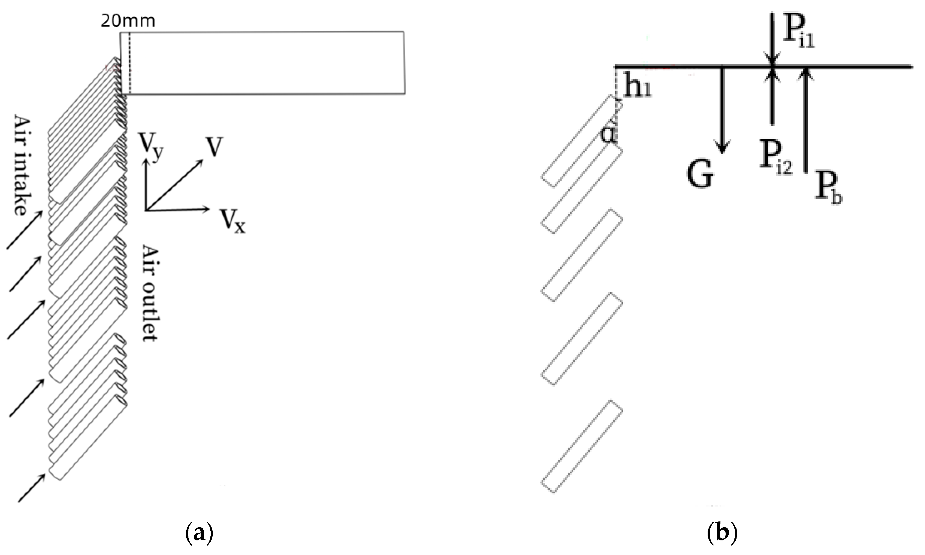
The main component of this research is a force analysis of the pipeline outlet on the conveyed object. In this paper, a pipeline with an inner diameter of 9 mm is the initial setting parameter; the pipeline model is simplified, and the force analysis of the related gas outlet is shown in Figure 1.
In fluid mechanics and aerodynamics [12], the ideal fluid follows the conservation of mechanical energy. Daniel Bernoulli proposed “Bernoulli’s principle” [13], which states that the pressure on the lower surface of the conveying object (total pressure P) is equal to the static pressure and the dynamic pressure. Dynamic pressure is the kinetic energy of air flowing in one direction. For an incompressible fluid, the Bernoulli Equation along the streamline is
where P is the static pressure, ρ is the fluid density, and V is the fluid velocity [14].
The dynamic pressure presented by the dynamic pressure energy to the outside is
There is a flow velocity in the direction parallel to the surface of the conveyed object, which means that the surface pressure on the lower surface of the conveyed object, as well as the static pressure, decreases. The static pressure difference between the upper surface and the lower surface causes the conveyed object to be under downward pressure; however, due to the increase in the dynamic pressure, the total pressure is also reduced. As such, the supporting object does not fall. To keep the conveying object balanced and not falling, the following equation needs to be satisfied:
Formulas (1)–(3) can be simplified as
It can be seen from Formula (4) that, if the equation is to be established, Vy needs to be greater than Vx, and the angle between the pipe and the box needs to be at least smaller than 45 °C. Therefore, the angle between each row of pipes and the box is initially set to be 40 °C. The length of the pallet is 20 mm, and the height of the first row of pipes from the pallet is about
Then, the pressure on the conveyed fabric is
First, the derivation and calculation are carried out with the gram weight ρ1 of the model fabric as 60 g/m2, because Vx = Vy × tanα1 and α1 = 40 °C, and the air gram weight is 1.29 kg/m3 by default. The above data are substituted into Formulas (1)–(5) to obtain Vx = 1.43 m/s, Vy = 1.70 m/s, ensuring that the flow velocity of the air x-direction parallel to the conveyed fabric is close to 1.43 m/s near the surface of the conveyed fabric, except for the boundary layer, so that the conveyed fabric can reach an equilibrium state.
2.2. Simulation Model and Meshing
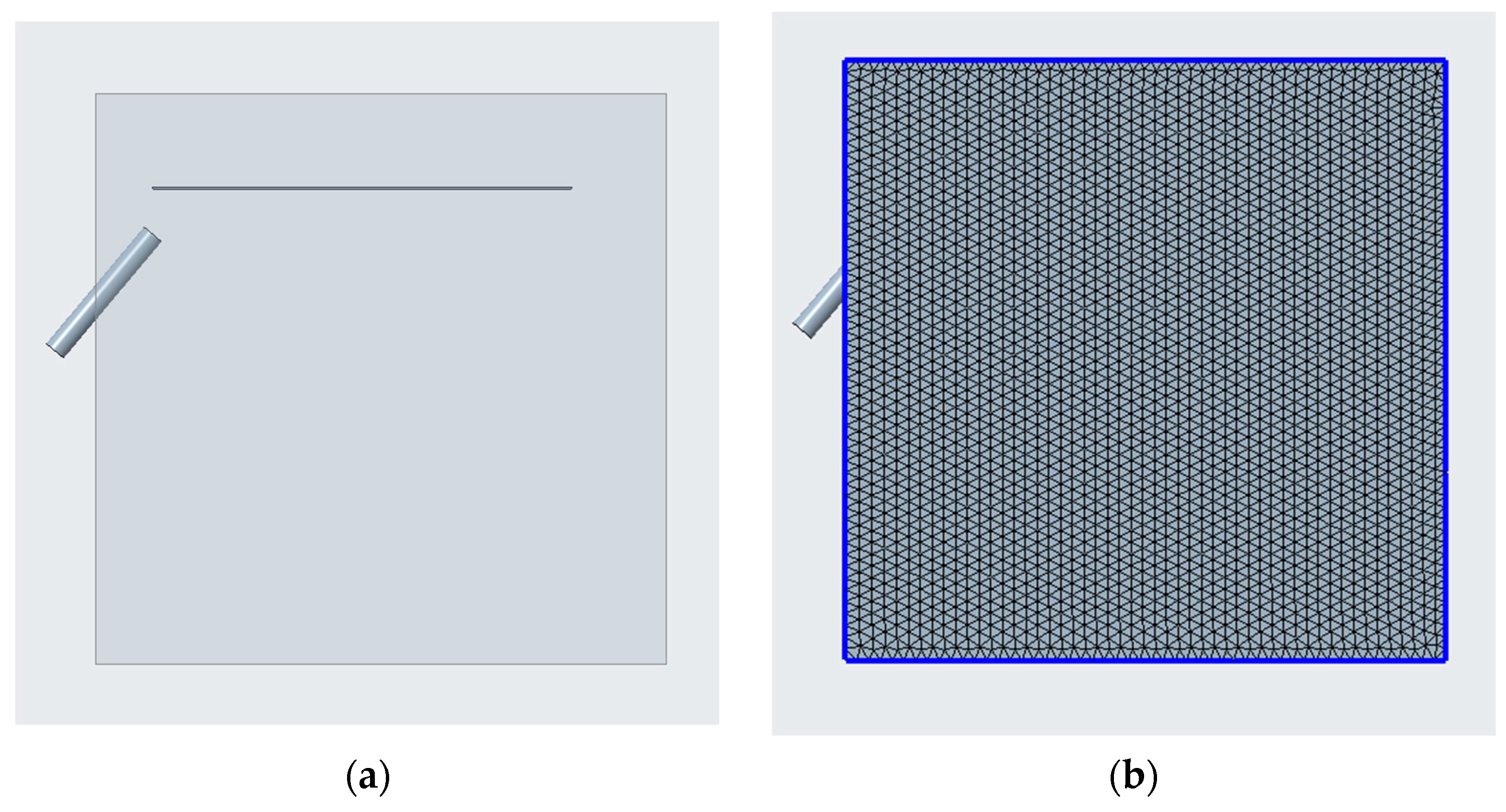
A conveying object model with a length of 220 mm (20 mm is the length of the pallet and 200 mm is the forward distance of the conveyed object) and a thickness of 1 mm is built. The center of the first row of pipes is 23.84 mm from the lower surface of the conveyed object, the angle is 40 °C, and the inner diameter of the pipe is 9 mm, with a wall thickness of 3 mm. This model involves the simultaneous simulation of the inner domain of the pipeline and the outer domain of the conveyed material. It is necessary to establish a simulation domain of the outer domain of the conveying object and the inner domain of the pipeline for mesh division, as shown in Figure 2.
2.3. Turbulent Kinetic Energy and the Turbulent Dissipation Rate
There are a large number of turbulent flows in nature. This kind of flow is very complex, and it has significant practical applications. The laminar flow is stable and forms turbulent flow. The most obvious feature of turbulence is its randomness [15]. The gas-assisted model is not only affected by many factors, such as the Reynolds number and incoming turbulence intensity, but these influencing factors are also interrelated and restrict each other [16]. In the process whereby the air enters the outside through the pipe and then exerts pressure on the conveyed fabric to prevent it from falling, it must first be considered whether the flow state of the air is turbulent or laminar [17]. Through the criterion of the flow state—the critical Reynolds number—the flow Reynolds number Re can be calculated and compared with the critical Reynolds number to judge the flow state [18]. The formula for the flow Reynolds number is
where ρ is the density of the fluid, v is the velocity of the fluid, L is the characteristic length, and μ is the viscosity coefficient. ρ is 1.29 kg/m3, L is 220 mm, and μ is 1.46 × 10⁻⁵ Pa·s. [19].
The above data can be substituted into the formula to obtain the Reynolds number:
The critical Reynolds number is 4300, judgment criteria by fluid state, when the Reynolds number exceeds 4300, it can be determined that the fluid state is turbulent at this time. Turbulence intensity describes the degree of wind speed change with time and space; it reflects the relative intensity of the fluctuating wind speed and is the most important characteristic quantity for describing the characteristics of atmospheric turbulence [20].
There are two main reasons for turbulence. One is that, when the air is flowing, it will be rubbed or blocked by the ground’s roughness. The other is the vertical movement of the airflow caused by the difference in the air weight and atmospheric temperature [21]. According to experience, turbulence intensity can be solved using the following formula:
Studying the laws of turbulent motion plays an increasingly important role in solving practical turbulence problems [22]. Accurately solving the turbulent flow field has always been one of the main goals of fluid mechanics. The turbulent kinetic energy is estimated by using the turbulence intensity above as
When the turbulent kinetic energy is transferred from the outer scale to the inner scale and reaches a dynamic equilibrium, the turbulent kinetic energy dissipation rate can be estimated by the flux of the turbulent kinetic energy in the inertial subregion [23]. The turbulence scale is estimated as
See Table 1 for the first simulation input data of the first pipeline.
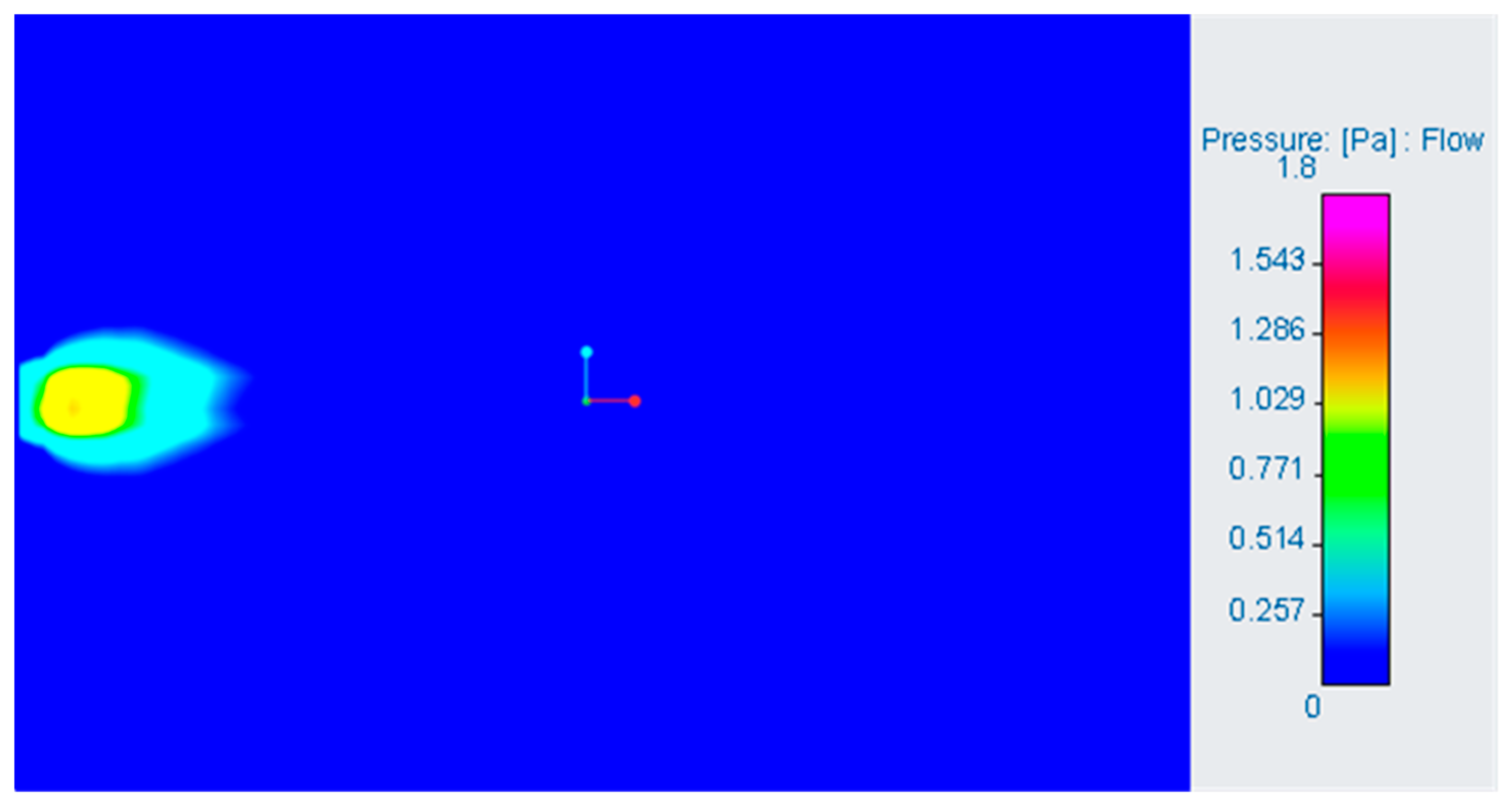
The pressure distribution obtained from the simulation is shown in Figure 3.
2.4. Boundary Layer Calculation with Monitoring Point Setting
The advantage of Creo fluid simulation is that it can be modeled and simulated directly in Creo. To observe the air flow rate on the lower surface of the conveyed material [24], it is necessary to set up several monitoring points.
According to the boundary layer theory proposed by Prandtl, for a fluid with low viscosity such as air, when the incoming Reynolds number is large enough, the influence of viscosity is limited to the thin layer of fluid near the surface area of the flowing object; the flow characteristics and the ideal flow are very different, and there is a large velocity gradient along the normal direction. The thin layer where the viscous force plays an important role in the near region of the object surface is the boundary layer [25]. Due to the adhesion conditions between the fluid and the object's surface, the velocity of the fluid in direct contact with the object surface drops to zero. In the subsequent simulation, the speed monitoring point cannot be set on the surface of the conveyed fabric, and the distance from the monitoring point to the lower surface of the conveyed material should be greater than the thickness of the boundary layer.
Due to the complexity of turbulence itself and the limitations of experimental measurement techniques [26], the thickness of the boundary layer can only be estimated based on the same magnitude of the viscous and inertial forces in the boundary layer in aerodynamics. For the flow around a plate, the relationship between the thickness of the boundary layer and the length of the plate is
Blasius’s exact solution formula for the boundary layer is
where δ is the boundary layer’s thickness, L is the length of the flat object, V∞ is the incoming velocity of the air, and v is the kinematic viscosity coefficient [27].
After measuring, the maximum distance that the airflow swept across the conveyed object is determined to be 40.70 mm. It can be calculated by substituting into the calculation formula the thickness of the Blasius boundary layer:
Therefore, the thickness of the boundary layer after the first pipe is discharged should be 2.91 mm, and the monitoring point should be set at 3.22 mm, as this is the best monitoring position.
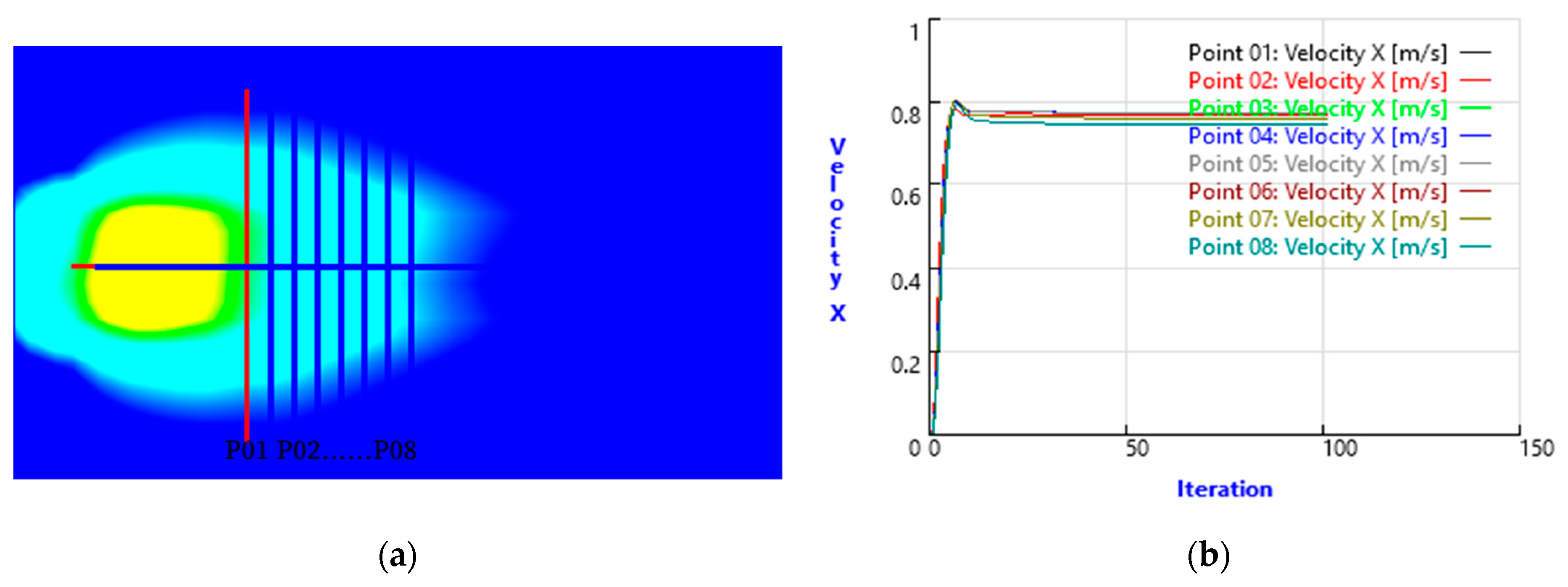
At a distance of 3.22 mm from the lower surface, eight monitoring points (P01–P08) are set along the center line of the conveyed object, with a spacing of 2 mm, and they are arranged in sequence. The speed of each monitoring point in the x-direction is shown in Figure 4.
3. Simulation and Data Analysis
3.1. Determination of the Outlet Velocity of the Pipeline
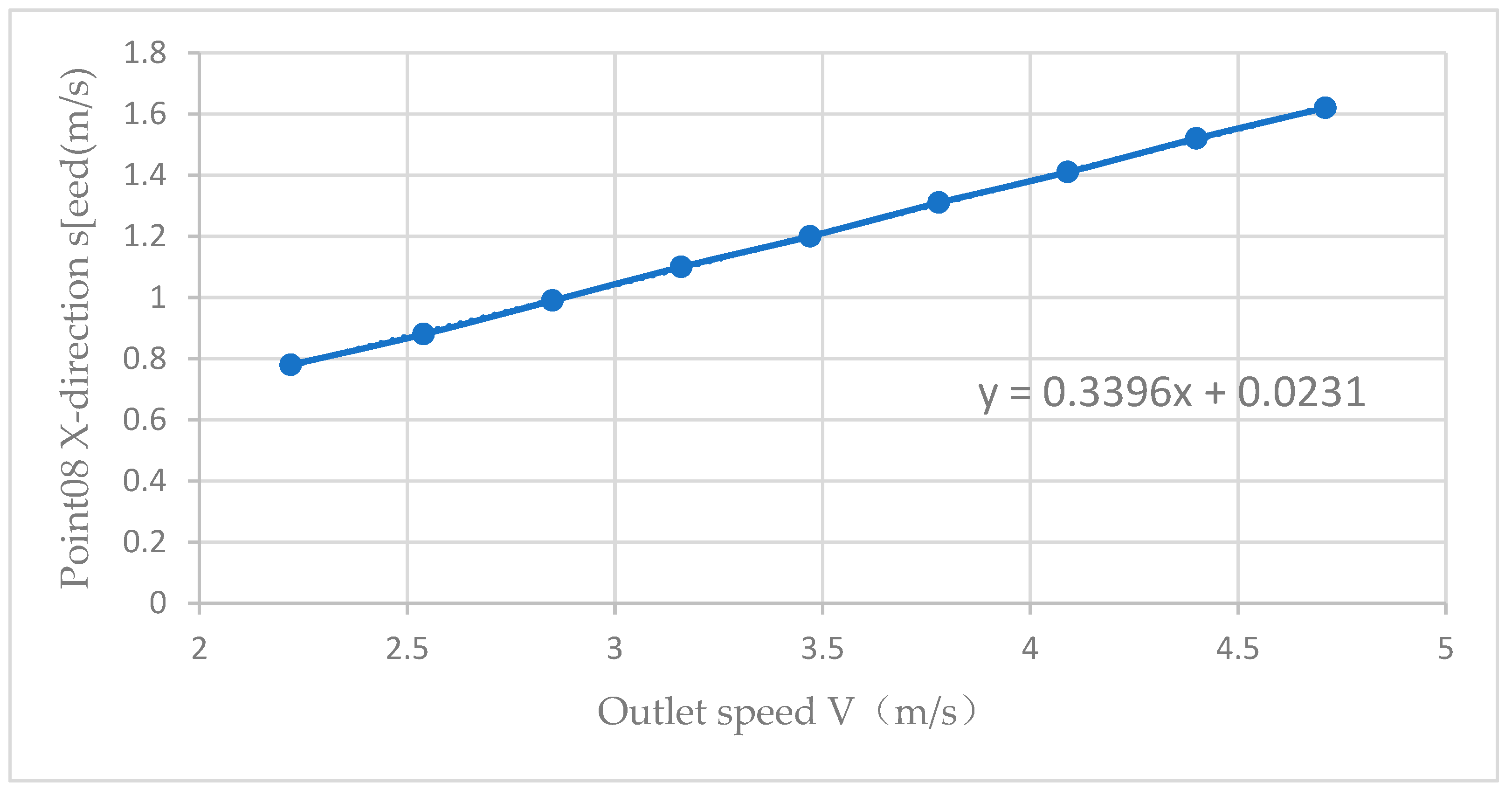
It is observed from Figure 4 that the maximum speed point P8 in the X-irection is 1.06 m/s, which is different from the obtained ideal speed in the x-direction of 1.43 m/s. This is because of the dissipation of turbulent energy in practice. At this time, the velocity of the air outlet can be adjusted so that the air velocity in the x-direction at the boundary layer approaches 1.76 m/s. The adjustment speed and the speed change of the maximum speed point P8 are shown in Table 2.
It can be seen from the figure that there is a linear trend, and a linear equation is obtained.
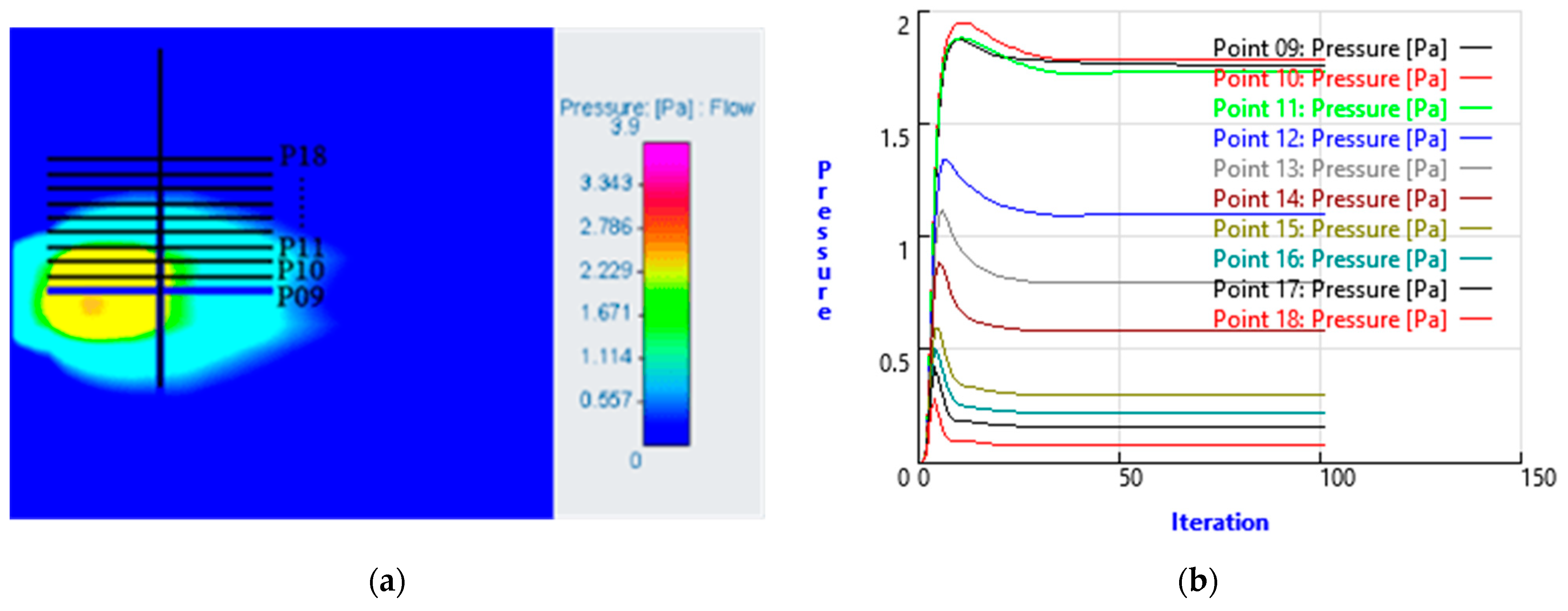
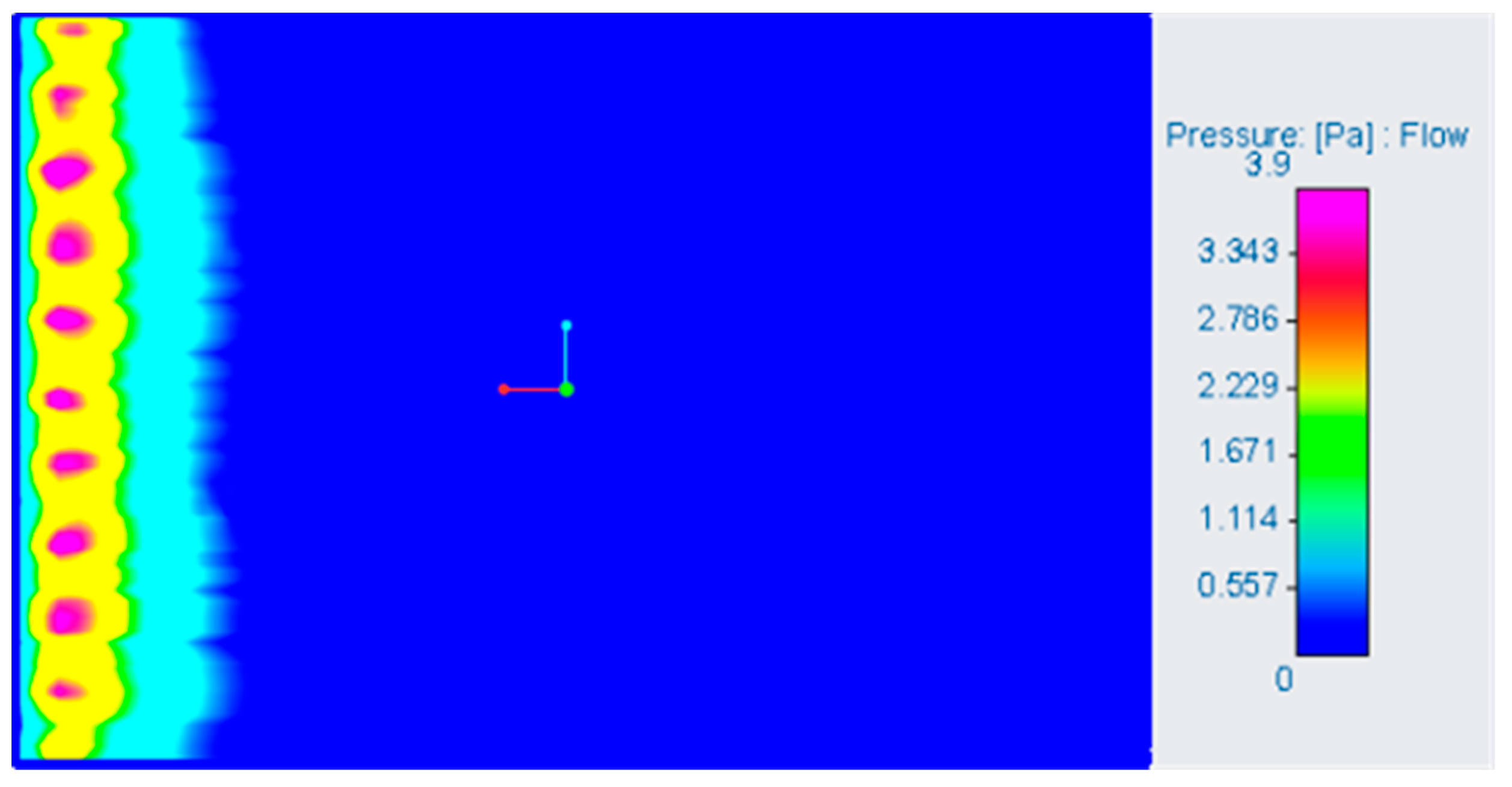
From this, to obtain the speed of 1.43 m/s in the x-direction of the P8 point, it is substituted into the linear equation to solve x = 4.14 m/s; the flow velocity in the x-direction of the air outlet is 2.66 m/s, and that in the y-direction is 3.17 m/s. When the x-direction of the P8 point is 3.17 m/s, the speed is close to 1.43 m/s. According to the cloud diagram of the pressure distribution on the lower surface of the conveyed fabric, as shown in Figure 6, ten monitoring points (P9–P18) are generated along the z-direction with a distance of 2 mm point pressure value. The pressure between points P16 and P17 tends to 0 pa, and the distance from the center line is about 14–16 mm. In order to ensure uniform lateral pressure distribution, the point of the minimum pressure value in the z-direction should be as close as possible to the point of the maximum pressure value. Considering the uniform distribution of each row of pipes, 11 pipes should be placed in the first row, as shown in Figure 7 for the simulation.
3.2. Determination of Pipeline Arrangement and Distribution
In the simulation in Figure 6, it can be deduced that the maximum pressure point is on the 20 mm pallet, which is a certain distance from the intersection of the pipe center line and the lower surface. According to the statistics of the pressure data, the maximum pressure point is about 8 mm away from the intersection of the pipe center line and the lower surface. It can be assumed that the maximum pressure point on the lower surface of the conveyed object should be 8 mm away from the intersection of the center line of the second pipe, and the lower surface after the second pipe is discharged. From this, it can also be concluded that the minimum pressure on the bottom surface of the first pipe is 40.70 mm. In order to keep the entire conveying object as constant and stable as possible, the maximum pressure point after the gas outlet of the second pipe and the minimum pressure point after the gas outlet of the first pipe should be coincident. Assuming that the included angle between each row of pipes and the box is 40 °C, the distance between the second row of pipes and the lower surface of the conveying object is
The first row of pipeline steps is repeated to simulate and analyze the calculations. Due to the distance from the lower surface, the pressure distribution on the lower surface of the conveying object increases with the vertical distance from the pipeline to the conveying object; the range also expands, but the pressure decreases. The thickness of the boundary layer formed by the output air flow of different rows of pipes to the lower surface of the conveying object is different. The calculation formula of the thickness of the boundary layer of the flat laminar flow can be obtained by Blasius, as shown in Table 3:
3.3. Surface Pressure Distribution under the Conveyed Material
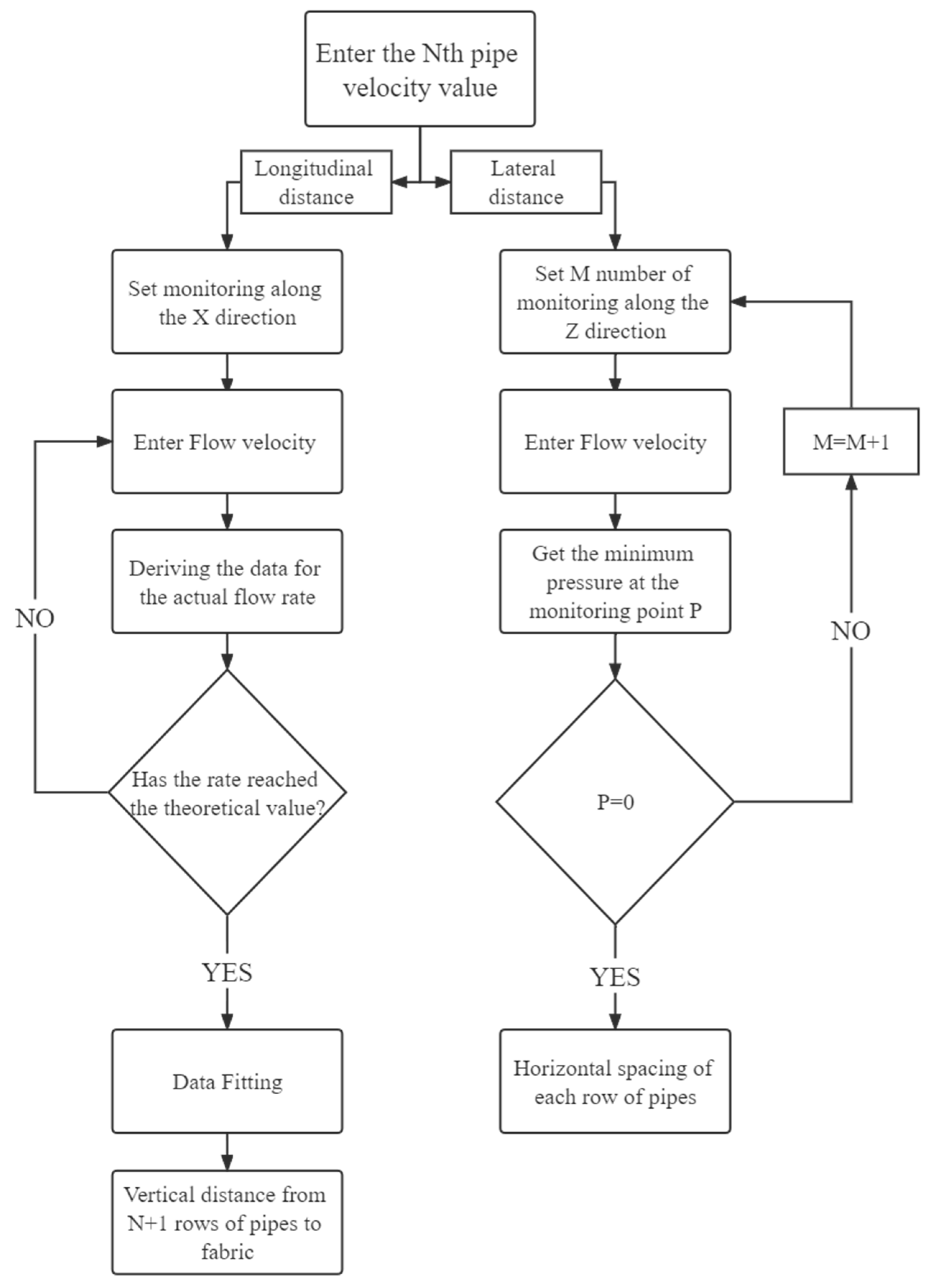
The parameters and arrangement of the second, third, fourth, and fifth rows of pipelines can be obtained according to the calculation flow chart of each row of pipeline parameters in Figure 8. The specific results are shown in Table 4.
The simulation analysis results of each row of pipelines, corresponding to the data in Table 4.
There are errors in the length and calculation of the gas flowing through the fabric in practice that affect the calculation of boundary layer thickness. The error graph is shown in Figure 9.
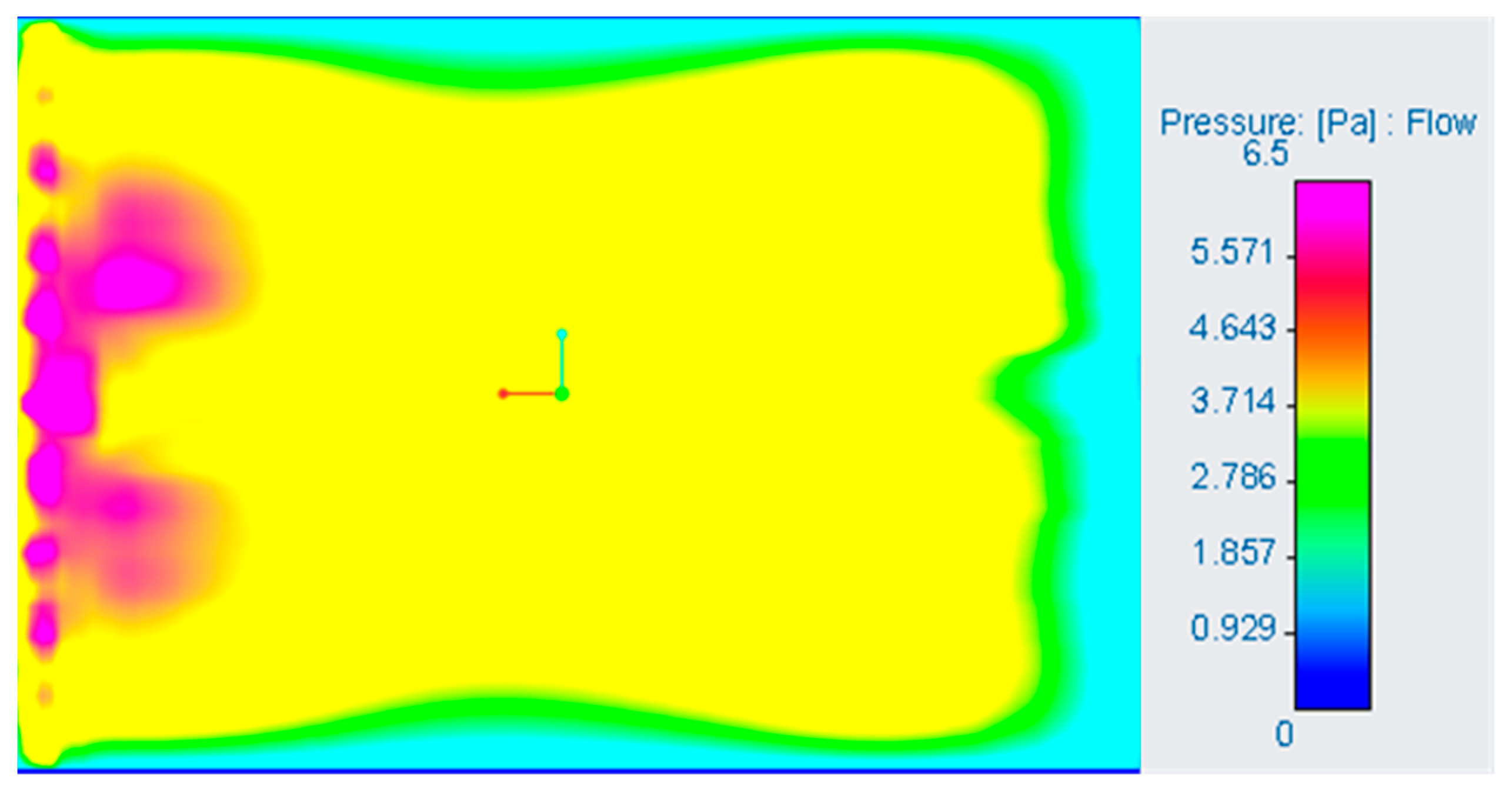
The final model building and meshing are shown in Figure 12. The pressure distribution formed on the lower surface of the conveyed object, after all the pipes output airflow together, is shown in Figure 13.
It can be observed that the surface pressure of the conveyed stream tends to be equal, overall. It is speculated, when the boundary pressure of the conveyed stream is small, this is because the airflow “flows out” at the boundary, and the boundary velocity accelerates, resulting in a decrease in the peripheral pressure. This hypothesis will be subject to further research in the future.
4. Discussion of the Demand Law
4.1. Theoretical Value of the Gas Flow Rate Required for Fabrics with Different Grammages
According to the (5) force balance equation, it can be simplified as
where ρ is the air weight, with a default value of 1.29 kg/m3; ρ1 is the conveyed fabric weight, for which different conveyed fabric weights are selected (the thin silk fabric weight range is 20–80 g/m2): 30, 40, 50, 70, and 80 g/m2. The theoretical value of the required gas flow rate for different grammage fabrics is shown in Table 5.
The angle between the pipe and the box, the diameter of the pipe, and the distance between the pipes remain unchanged. Creo is used to simulate and adjust the pipe outlet in sequence.
4.2. Simulation Adjustment of the Conveyed Fabric under Different Gram Weights
According to Section 2.4, having determined the boundary layer thickness of each row of the pipeline output airflow on the lower surface of the conveyed fabric and set up monitoring points, the value changes in the monitoring points are observed, and the flow velocity is adjusted at the outlet of the pipeline, so that the flow velocity at the monitoring point is close to the theoretical value. The thickness of the boundary layer after the air outlet of each row of pipes under conveyed fabrics with different gram weights is shown in Table 6.
The flow rate of each row of pipelines for different grammage fabric requirements is summarized in Table 7.
The airflow formula is
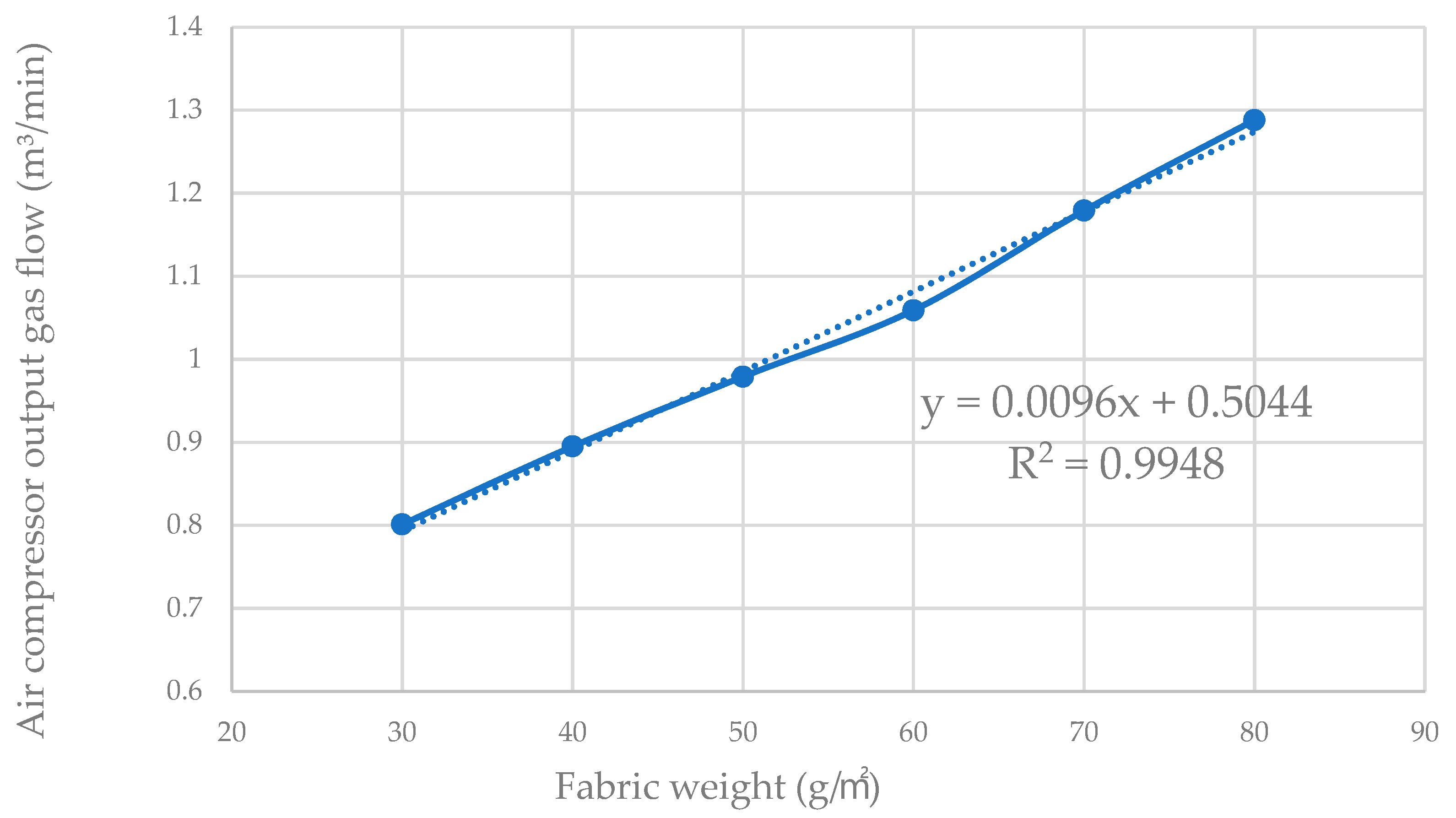
The total flow of the air compressor is calculated, and data fitting is conducted, as shown in Figure 15.
The simulation results of this study are roughly the same as the expected results, and the pressure on the lower surface of the fabric is evenly distributed. The simulation results are roughly the same for different fabric weights. At the same time, it was found that the pressure at the boundary of the lower surface of the fabric is relatively small. It is speculated that the reason for this may be that the air velocity at the boundary increases significantly, resulting in a decrease in the peripheral pressure. The shortcoming of this study is that the fabric deformation, and the effect of this deformation on the airflow, are not considered. In future studies, the degree of fabric deformation and the coupling of the fabric to the airflow will be considered. At the same time, in the fluid simulation, the fluid–solid coupling effect needs to be considered, which is also a very critical influencing factor. The findings of this study will be widely used in the future, and are of great significance to the feeding mechanisms in the home textile industry.
5. Conclusions
- (1)
- A scheme for the gas-assisted conveying of flexible materials was proposed, For the first time, in the passage to the outside world, the use of air force to transport the fabric, and a mathematical model of the balance between the upper and lower surfaces of conveyed flexible materials was deduced.
- (2)
- A gas-assisted conveying mechanism model for the pneumatic conveying of flexible materials was established, and the surface pressure distribution for conveying flexible materials was simulated and analyzed using the Creo flow analysis module. The minimum pressure point of the conveyed fabric in the Z-direction was superimposed with the adjacent maximum pressure point after the air is discharged between the same row of single pipes, and then, superimposed to determine the distance between the upper and lower adjacent rows, so as to determine the horizontal spacing.
- (3)
- The layout scheme of a total of 41 pipes in five rows was determined. The tubes are 9 mm in diameter and arranged in five rows. From the first row to the fifth row, there are 11, 9, 8, and 7 pipes, respectively. The constructed gas-assisted conveying mechanism model can not only realize the smooth lifting and forward conveying of the conveyed flexible materials, but also provides a reference for the development of a new feeding mechanism for automatic sewing and cutting machines.
- (4)
- This paper deduced and analyzed the changing law of the gas flow rate demand of each row of pipelines in the gas-assisted model for different grammage fabrics. It also summarized the demand law of different grammage fabrics for the output flow of the air compressor, developing three-side automatic sewing cutting for the next generation of home textile kits and providing a reference for the development of integrated devices.
6. Patents
The authors of this paper have carried out research on home-textile-kit automatic sewing and cutting integrated devices for many years. Four Chinese invention patents related to this paper have been published; the Patent Application Publication numbers are CN 111847032 A, CN 111824814 A, CN 110424104 A, and CN 110409067 A. Significantly, two patent authorization announcements have been granted; the patent numbers are CN 110409067 B and CN 110344184 B.
Author Contributions
Conceptualization, J.Z. and X.W.; methodology, J.Z. and Y.Z.; software, validation, and formal analysis, J.Z.; investigation, X.W. and J.Z.; resources, H.N.; data curation, J.Z.; writing—original draft preparation, J.Z.; writing—review and editing, X.W. and Y.Z.; visualization, X.W.; supervision, J.Z.; project administration, Y.Z.; funding acquisition, H.N. and X.W. All authors have read and agreed to the published version of the manuscript.
Funding
This research was supported by a project funded by the Priority Academic Program Development scheme of Jiangsu Higher Education Institutions (grant No. PAPD), and the Jiangsu Provincial Key Research and Development Program of China (grant No. BE2021065).
Institutional Review Board Statement
Not applicable.
Informed Consent Statement
Not applicable.
Data Availability Statement
Not applicable.
Conflicts of Interest
The authors declare no conflict of interest.
References
- Jiang, D. Analysis and matching designs of the home textile decorative art. Agro Food Ind. Hi-Tech 2017, 28, 2785–2789. [Google Scholar]
- Yuliastuti, G.E.; Rizki, A.M.; Mahmudy, W.F.; Tama, I.P. Determining Optimum Production Quantity on Multi-Product Home Textile Industry by Simulated Annealing. J. Inf. Technol. Comput. Sci. 2018, 3, 159–168. [Google Scholar] [CrossRef] [Green Version]
- Meng, X.; Han, Y.; Chen, Z.; Ghaffar, A.; Chen, G. Aerodynamic Effects of Ceiling and Ground Vicinity on Flapping Wings. Appl. Sci. 2022, 12, 4012. [Google Scholar] [CrossRef]
- Couto, N.; Bergada, J.M. Aerodynamic Efficiency Improvement on a NACA-8412 Airfoil via Active Flow Control Implementation. Appl. Sci. 2022, 12, 4269. [Google Scholar] [CrossRef]
- Dos Santos, J.D.; Anjos, G.R.; Savi, M.A. An investigation of fluid-structure interaction in pipe conveying flow using reduced-order models. Meccanica 2022, 57, 2473–2491. [Google Scholar] [CrossRef]
- Markauskas, D.; Platzk, S.; Kruggel-Emden, H. Comparative numerical study of pneumatic conveying of flexible elongated particles through a pipe bend by DEM-CFD. Powder Technol. 2022, 399, 117170. [Google Scholar] [CrossRef]
- Nowak, J.L.; Siebert, H.; Szodry, K.; Malinowski, S.P. Coupled and decoupled stratocumulus-topped boundary layers: Turbulence properties. Atmos. Chem. Phys. 2021, 21, 10965–10991. [Google Scholar] [CrossRef]
- PTC. Creo 7.0 Generative Design and New Functions of Simulation. Intell. Manuf. 2020, 5, 23–27. [Google Scholar]
- Al-Obaidi, A.R.; Mohammed, A.A. Numerical Investigations of Transient Flow Characteristic in Axial Flow Pump and Pressure Fluctuation Analysis Based on the CFD Technique. J. Eng. Sci. Technol. Rev. 2019, 12, 6. [Google Scholar] [CrossRef]
- Al-Obaidi, A.R. Numerical investigation of flow field behaviour and pressure fluctuations within an axial flow pump under transient flow pattern based on CFD analysis method. J. Phys. Conf. Ser. 2019, 1279, 012069. [Google Scholar] [CrossRef] [Green Version]
- Shu, C.; Wang, L.L.; Mortezazadeh, M. Dimensional analysis of Reynolds independence and regional critical Reynolds numbers for urban aerodynamics. J. Wind Eng. Ind. Aerodyn. 2020, 203, 104232. [Google Scholar] [CrossRef]
- Kaliyeva, K. Energy Conservation Law for the Turbulent Motion in the Free Atmosphere: Turbulent Motion in the Free Atmosphere. In Handbook of Research on Computational Simulation and Modeling in Engineering; IGI Global: Hershey, PA, USA, 2016; pp. 105–138. [Google Scholar]
- Verma, M.K.; Kumar, A.; Kumar, P.; Barman, S.; Chatterjee, A.G.; Samtaney, R.; Stepanov, R.A. Energy spectra and fluxes in dissipation range of turbulent and laminar flows. Fluid Dyn. 2018, 53, 862–873. [Google Scholar] [CrossRef]
- Liu, P. Exploration and practice of aerodynamics seminar. Mech. Pract. 2016, 38, 87–89. [Google Scholar]
- Zhang, L.T.; Yang, J. Evaluation of aerodynamic characteristics of a coupled fluid-structure system using generalized Bernoulli’s principle: An application to vocal folds vibration. J. Coupled Syst. Multiscale Dyn. 2016, 4, 241–250. [Google Scholar] [CrossRef] [Green Version]
- Marusic, I.; Kunkel, G.J. Streamwise turbulence intensity formulation for flat-plate boundary layers. Phys. Fluids 2003, 15, 2461–2464. [Google Scholar] [CrossRef]
- Nguyen, T.H.T.; Park, S.; Jang, D.; Ahn, J. Evaluation of Three-Dimensional Environmental Hydraulic Modeling in Scour Hole. Appl. Sci. 2022, 12, 4032. [Google Scholar] [CrossRef]
- Rafner, J.; Grujić, Z.; Bach, C.; Bærentzen, J.A.; Gervang, B.; Jia, R.; Leinweber, S.; Misztal, M.; Sherson, J. Geometry of turbulent dissipation and the Navier–Stokes regularity problem. Sci. Rep. 2021, 11, 8824. [Google Scholar] [CrossRef]
- Končar, B.; Sotošek, J.; Bajsić, I. Experimental verification and numerical simulation of a vortex flowmeter at low Reynolds numbers. Flow Meas. Instrum. 2022, 88, 2378. [Google Scholar] [CrossRef]
- Yang, W.; Yue, H.; Deng, E.; Wang, Y.; He, X.; Zou, Y. Influence of the turbulence conditions of crosswind on the aerodynamic responses of the train when running at tunnel-bridge-tunnel. J. Wind Eng. Ind. Aerodyn. 2022, 229, 105138. [Google Scholar] [CrossRef]
- Beaulac, P.; Issa, M.; Ilinca, A.; Brousseau, J. Parameters Affecting Dust Collector Efficiency for Pneumatic Conveying: A Review. Energies 2022, 15, 916. [Google Scholar] [CrossRef]
- Yang, D.; Wang, Y.; Hu, Z. Research on the pressure dropin horizontal pneumatic conveying for large coal particles. Processes 2020, 8, 650. [Google Scholar] [CrossRef]
- Thakur, N.; Murthy, H. Simulation study of droplet formation in inkjet printing using ANSYS FLUENT. J. Phys. Conf. Ser. 2022, 2161, 012026. [Google Scholar] [CrossRef]
- Zhao, H.; Ma, L. Study of Eco-evolution Path of Home Textile Industry under the Background of Internet Plus. J. Phys. Conf. Ser. 2021, 1910, 012061. [Google Scholar] [CrossRef]
- Kirillin, G.; Aslamov, I.; Kozlov, V.; Zdorovennov, R.; Granin, N. Turbulence in the stratified boundary layer under ice: Observations from Lake Baikal and a new similarity model. Hydrol. Earth Syst. Sci. 2020, 24, 1691–1708. [Google Scholar] [CrossRef] [Green Version]
- Vallis, G.K. Turbulence theory: Imperfect, but necessary. AGU Adv. 2021, 2, e2020AV000362. [Google Scholar] [CrossRef]
- Escott, L.J.; Griffiths, P. Revisiting boundary layer flows of viscoelastic fluids; J. Non-Newton. Fluid Mech. Online 2022, 104, 104976. [Google Scholar] [CrossRef]
Figure 1.
Force analysis of the pipeline outlet and transported logistics: (a) pipeline outlet diagram; (b) force diagram of the conveyed logistics.
Figure 1.
Force analysis of the pipeline outlet and transported logistics: (a) pipeline outlet diagram; (b) force diagram of the conveyed logistics.

Figure 2.
Inner and outer domain meshing: (a) simulation of the internal and external domains; (b) mesh division.
Figure 2.
Inner and outer domain meshing: (a) simulation of the internal and external domains; (b) mesh division.

Figure 3.
Surface pressure under conveying stream.

Figure 4.
Monitoring point distribution map and x-direction speed curve: (a) monitoring point settings; (b) speed in x-direction at each point.
Figure 4.
Monitoring point distribution map and x-direction speed curve: (a) monitoring point settings; (b) speed in x-direction at each point.

Figure 5.
P08 point x-direction speed scatter diagram and fitting curve.

Figure 6.
The first row of single pipe pressure: (a) distribution of monitoring points in the z-direction; (b) pressure distribution at each point.
Figure 6.
The first row of single pipe pressure: (a) distribution of monitoring points in the z-direction; (b) pressure distribution at each point.

Figure 7.
Pressure distribution of the first row of pipes.

Figure 8.
Calculation flow chart of the pipeline parameters of each row.

Figure 9.
Airflow through fabric distance error.

Figure 10.
Pressure distribution diagram of each row of single pipes after the air outlet: (a) the second row of single longitudinal pipes; (b) the third row of single longitudinal pipes; (c) the fourth row of single longitudinal tubes; (d) the fifth row of single longitudinal tubes.
Figure 10.
Pressure distribution diagram of each row of single pipes after the air outlet: (a) the second row of single longitudinal pipes; (b) the third row of single longitudinal pipes; (c) the fourth row of single longitudinal tubes; (d) the fifth row of single longitudinal tubes.

Figure 11.
Pressure distribution diagram of all pipes in each row after the air outlet: (a) the second row of horizontal pipes; (b) the third row of horizontal pipes; (c) the fourth row of horizontal pipes; (d) the fifth row of horizontal pipes.
Figure 11.
Pressure distribution diagram of all pipes in each row after the air outlet: (a) the second row of horizontal pipes; (b) the third row of horizontal pipes; (c) the fourth row of horizontal pipes; (d) the fifth row of horizontal pipes.

Figure 12.
Modeling and meshing of the final solution: (a) modeling of the final solution; (b) meshing of the final model.
Figure 12.
Modeling and meshing of the final solution: (a) modeling of the final solution; (b) meshing of the final model.

Figure 13.
Cloud map of the final pressure distribution.

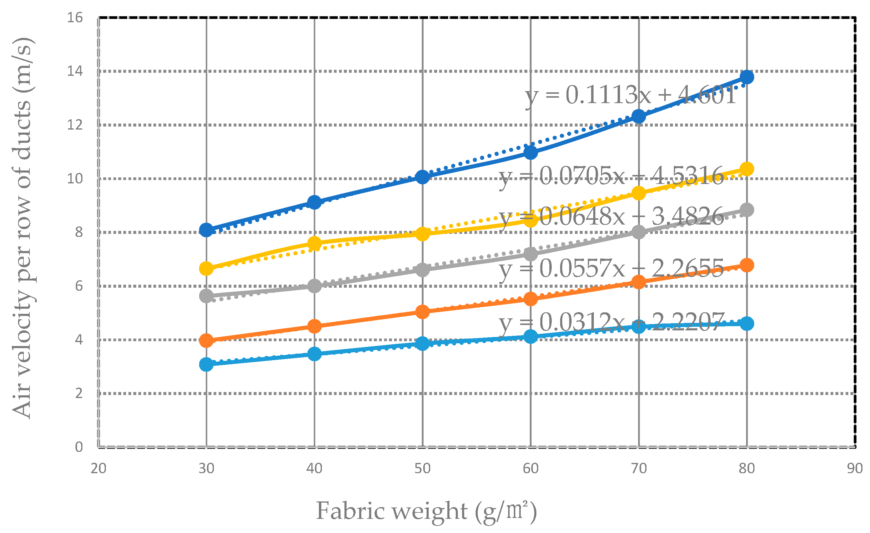
Figure 14.
The relationship between the airflow rate of each row of ducts and the weight of the fabric.
Figure 14.
The relationship between the airflow rate of each row of ducts and the weight of the fabric.

Figure 15.
Fitting the relationship between the total flow and the gram weight of the conveyed fabric.
Figure 15.
Fitting the relationship between the total flow and the gram weight of the conveyed fabric.


Table 1.
Simulation parameters.
| Simulation Parameters | Value |
|---|---|
| Pipe outlet speed in x-direction Vx (m/s) | 1.43 |
| Pipe outlet y-direction speed Vy (m/s) | 1.70 |
| Turbulent kinetic energy (m3/s2) | 0.00341 |
| Turbulent kinetic energy dissipation rate (m2/s2) | 0.0102 |
Table 2.
Speed in x-direction at point P08 at different flow rates.
| Experiment Number | 1 | 2 | 3 | 4 | 5 | 6 | 7 | 8 | 9 |
|---|---|---|---|---|---|---|---|---|---|
| Air outlet x-direction speed Vx (m/s) | 1.43 | 1.63 | 1.83 | 2.03 | 2.23 | 2.43 | 2.63 | 2.83 | 3.03 |
| Air outlet y-direction speed Vy (m/s) | 1.70 | 1.94 | 2.18 | 2.42 | 2.66 | 2.90 | 3.13 | 3.37 | 3.61 |
| outlet speed V (m/s) | 2.22 | 2.54 | 2.85 | 3.16 | 3.47 | 3.78 | 4.09 | 4.40 | 4.71 |
| Point 08 x-direction speed (m/s) | 0.78 | 0.88 | 0.99 | 1.10 | 1.20 | 1.31 | 1.41 | 1.52 | 1.62 |
Table 3.
Boundary layer thickness of each row of pipes.
| Row of Pipes | The Distance That the Airflow Swept across the Conveyed Object L (mm) | Boundary Layer Thickness (mm) |
|---|---|---|
| 1 | 40.70 | 3.22 |
| 2 | 71.49 | 4.27 |
| 3 | 94.55 | 4.91 |
| 4 | 114.98 | 5.41 |
| 5 | 105.86 | 5.20 |
Table 4.
Overall piping arrangement.
| Row of Pipes | Number of Pipes | Vertical Distance to Conveyed Object H (mm) | Airflow Rate in the Pipe V (m/s) |
|---|---|---|---|
| 1 | 11 | 23.84 | 4.20 |
| 2 | 9 | 58.03 | 5.02 |
| 3 | 8 | 108.64 | 8.48 |
| 4 | 7 | 170.79 | 9.99 |
| 5 | 6 | 250.78 | 13.78 |
Table 5.
Theoretical flow rate of the air outlet when the conveyed fabric has different gram weights.
Table 5.
Theoretical flow rate of the air outlet when the conveyed fabric has different gram weights.
| Conveyed Fabric Weight (g/m2) | 30 | 40 | 50 | 60 | 70 | 80 |
|---|---|---|---|---|---|---|
| Theoretical air velocity in the x-direction (m/s) | 1.04 | 1.20 | 1.34 | 1.43 | 1.60 | 1.43 |
| Theoretical air velocity in y-direction (m/s) | 1.24 | 1.43 | 1.60 | 1.70 | 1.90 | 2.10 |
Table 6.
Boundary layer thickness of the gas flowing through the lower surfaces of different fabrics.
Table 6.
Boundary layer thickness of the gas flowing through the lower surfaces of different fabrics.
| Conveyed Fabric Weight (g/m2) | 30 | 40 | 50 | 60 | 70 | 80 |
|---|---|---|---|---|---|---|
| Boundary layer thickness of the first row of pipes (mm) | 3.78 | 3.52 | 3.33 | 3.22 | 3.05 | 2.91 |
| Boundary layer thickness of the second row of pipes (mm) | 5.00 | 4.66 | 4.41 | 4.27 | 4.04 | 3.85 |
| Boundary layer thickness of the third row of pipes (mm) | 5.76 | 5.36 | 5.07 | 4.91 | 4.64 | 4.43 |
| Boundary layer thickness of the fourth row of pipes (mm) | 6.35 | 5.91 | 5.60 | 5.41 | 5.12 | 4.88 |
| Boundary layer thickness of the fifth row of pipes (mm) | 6.10 | 5.67 | 5.37 | 5.20 | 4.91 | 4.69 |
Table 7.
The flow velocity of each row of pipe outlet under different fabric weights.
| Conveyed Fabric Weight (g/m2) | 30 | 40 | 50 | 60 | 70 | 80 |
|---|---|---|---|---|---|---|
| The flow velocity of the first row of pipes Vi1 (m/s) | 3.08 | 3.47 | 3.86 | 4.12 | 4.49 | 4.60 |
| The flow velocity of the second row of pipes Vi2 (m/s) | 3.97 | 4.50 | 5.04 | 5.52 | 6.15 | 6.78 |
| The flow velocity of the third row of pipes Vi3 (m/s) | 5.63 | 6.00 | 6.60 | 7.19 | 8.01 | 8.84 |
| The flow velocity of the fourth row of pipes Vi4 (m/s) | 6.65 | 7.59 | 7.94 | 8.45 | 9.46 | 10.36 |
| The flow velocity of the fifth row of pipes Vi5 (m/s) | 8.09 | 9.12 | 10.06 | 10.97 | 12.32 | 13.78 |
Disclaimer/Publisher’s Note: The statements, opinions and data contained in all publications are solely those of the individual author(s) and contributor(s) and not of MDPI and/or the editor(s). MDPI and/or the editor(s) disclaim responsibility for any injury to people or property resulting from any ideas, methods, instructions or products referred to in the content. |
© 2023 by the authors. Licensee MDPI, Basel, Switzerland. This article is an open access article distributed under the terms and conditions of the Creative Commons Attribution (CC BY) license (https://creativecommons.org/licenses/by/4.0/).
Share and Cite
MDPI and ACS Style
Zhu, Y.; Zhai, J.; Ni, H.; Wang, X. Demand Law of Fabric Weight on the Airflow Velocity of a Gas-Assisted Model. Appl. Sci. 2023, 13, 912. https://doi.org/10.3390/app13020912
AMA Style
Zhu Y, Zhai J, Ni H, Wang X. Demand Law of Fabric Weight on the Airflow Velocity of a Gas-Assisted Model. Applied Sciences. 2023; 13(2):912. https://doi.org/10.3390/app13020912
Chicago/Turabian StyleZhu, Yu, Jianzhou Zhai, Hongjun Ni, and Xingxing Wang. 2023. "Demand Law of Fabric Weight on the Airflow Velocity of a Gas-Assisted Model" Applied Sciences 13, no. 2: 912. https://doi.org/10.3390/app13020912
Note that from the first issue of 2016, this journal uses article numbers instead of page numbers. See further details here.