Open-Set Signal Recognition Based on Transformer and Wasserstein Distance

Featured Application

Signal Processing.

Abstract

Open-set signal recognition provides a new approach for verifying the robustness of models by introducing novel unknown signal classes into the model testing and breaking the conventional closed-set assumption, which has become very popular in real-world scenarios. In the present work, we propose an efficient open-set signal recognition algorithm, which contains three key sub-modules: the signal representation sub-module based on a vision transformer (ViT) structure, a set distance metric sub-module based on Wasserstein distance, and a class space compression sub-module based on reciprocal point separation and central loss. In this algorithm, the representing features of signals are established based on transformer-based neural networks, i.e., ViT, in order to extract global information about time series-related data. The employed reciprocal point is used in modeling the potential unknown space without using the corresponding samples, while the distance metric between different class spaces is mathematically modeled in terms of the Wasserstein distance instead of the classical Euclidean distance. Numerical experiments on different open-set signal recognition tasks show that the proposed algorithm can significantly improve the recognition efficiency in both known and unknown categories.

1. Introduction

Deep learning (DL), represented by the convolutional neural network (CNN), has recently made remarkable achievements in the field of signal recognition [1,2,3,4,5,6]. However, the over-reliance on massive labeled training data significantly limits its ability to solve practical signal recognition problems. Due to the assumption that the test classes are consistent with the classes from the training set, DL-based signal recognition models often fail in real-world scenarios if any unexplored and unknown class appears during the inference stage [3,7]. The key issue is whether, without having enough knowledge about the world with open space risk, our models can still perform well if any unseen and challenging scenario is encountered. This is termed the open-set signal recognition problem, which can be considered as the practical application of open-set recognition (OSR) [7,8,9,10] on signal processing.

The open-set signal recognition (OSSR) provides a new evaluation criterion to verify the robustness of models by introducing novel, unknown signal classes into the model testing and breaking the conventional closed-set assumption. For instance, the DL-based signal recognition methods are typically trained on signals observed from known objectives. But users usually receive signals from unknown objectives and expect the model to distinguish those “outside” signals simultaneously. More specifically, under the open-set assumption, signals can be split into four basic categories of known-known classes (KKCs), known-unknown classes (KUCs), unknown-known classes (UKCs), and unknown-unknown classes (UUCs) [7]. The goal of OSSR is to ensure that the model can successfully distinguish all the known signal classes received from the training set and reject all the unknown signal classes in the inference phase.

The traditional machine learning-based (TML-based) methods were proposed for solving open-set recognition problems (not limited to the OSSR problem), e.g., the compact abating probability (CAP) method to explicitly reduce the open space risk [10,11]. Some TML-based methods were proposed with various schemes, such as the sparse representation, extreme value, or hashing, to separate known and unknown classes [12,13,14,15,16,17,18]. In addition to the TML-based methods, the DL-based methods employ various deep learning models with well-designed losses and recognition functions to handle the open-set recognition. For example, the early typical DL-based open-set recognition method calibrates softmax scores and uses the extreme value theorem to detect outliers [19]. Furthermore, the DL-based methods have become the mainstream methods for the open-set recognition problem with a series of works [20,21,22,23,24,25,26]. More details can be found in the recent survey papers [7,27].

In the case of signal recognition problems, the premise of the DL-based method is to collect sufficient types and numerous quantities of signal data. However, it is difficult to collect enough samples for some signals, especially in the military field. Open set recognition has become more popular in real-world scenarios, where an incomplete knowledge of modulation types exists at the training time, and unknown classes are required to be classified during the testing. Unknown signals will appear in the testing set. However, the DL model can only classify them into the known classes with the highest probability score rather than treating them as unknowns. It becomes necessary to apply the open set theory to the OSSR problem in order to overcome the limitation of deep learning.

The zero-shot learning (ZSL) framework was proposed in [3] to address the OSSR problems, where the key idea is to learn a representation of the signal semantic feature space with the CNN structure, as well as to learn the well-designed losses and Mahalanobis distance metric. The learning with an emerging new class seems relevant to zero-shot learning, which is a hot topic in image classification and aims to classify those visual classes which did not appear the in the training data set. The zero-shot learning is assumed to work with side information, i.e., external knowledge, such as the class definitions, descriptions, or properties, that can help to associate the seen and unseen classes, and, hence, it can be treated as a kind of transfer learning. In contrast, learning with an emerging new class is a general machine learning setting that does not assume such external knowledge.

In this work, we propose an efficient open-set signal recognition algorithm named open-set signal recognition based on the transformer and Wasserstein distance (${\mathrm{OSSG}}_{TW}$). It contains three key sub-modules including signal representation, which is a sub-module based on ViT structure, the set distance metric sub-module based on Wasserstein distance, and the class space compression sub-module based on reciprocal point separation and central loss. In this algorithm, the representing features of signals are established based on the transformer-based neural networks, i.e., ViT, in order to extract the global information about the time series-related data. The employed reciprocal point is used to model the potential unknown space without the corresponding samples, and the distance metric between different class spaces is mathematically modeled in terms of the Wasserstein distance instead of the classical Euclidean distance. The main contributions of this work are as follows:

(1).

An efficient open-set signal recognition algorithm is proposed, which employs a reciprocal point and central loss to establish the signal classification procedure, especially for unknown categories;

(2).

Transformer-based structure and Wasserstein distance, which are creatively used to extract features and measure category distances, respectively;

(3).

Numerical experiments on different open-set signal recognition tasks are performed, which show that the proposed algorithm can significantly improve the recognition efficiency on both known and unknown categories.

The following is the roadmap of this paper. Section 2 summarizes the major related works on the open-set learning and signal recognition methods. Section 3 presents the preliminary knowledge for our work, followed by the proposed open-set signal recognition algorithm in Section 4. Comprehensive experiments on real signals are presented in Section 5.

2. Related Work

Recently, signal recognition via deep learning has achieved a series of successes. The convolutional radio modulation recognition network was proposed in [28], which can adapt itself to the complex temporal radio signal domain and also works well at low signal-to-noise ratios (SNRs). The residual neural network was employed in [2] to perform the signal recognition tasks across a range of configurations and channel impairments, offering referable statistics. Two convolutional neural networks, AlexNet and GoogLeNet, were used in [29] to address the modulation classification tasks by demonstrating the significant advantage of the deep learning-based approach in this field. Another deep learning-based big data processing architecture for the end-to-end signal processing task was proposed in [30] to obtain important information from radio signals. The adversarial evasion attacks, which lead to misclassification in the context of wireless communications, were evaluated in [31]. Further, an automatic multiple multicarrier waveform classification was introduced in [32], which can use the principal component analysis to suppress the additive white Gaussian noise and reduce the input dimensions of CNNs. Some other CNN-based signal recognition algorithms were also proposed to demonstrate the efficient recognition ability [33,34,35].

In summary, deep learning-based open-set recognition methods can be categorized into two groups: discriminative model-based methods and generative model-based methods. The discriminative model-based methods calibrate the classification logistics to detect UUCs. The typical OpenMax [19] employed an OpenMax layer and output probabilities with Weibull distributions. On the basis of OpenMax, CROSR [23] performed more encoding processing on the original sample x by rebuilding the sample to improve the performance of the method in the open set scenarios. In addition, there are some methods to improve on OpenMax, such as DOC [23], COOL [36], C2AE [37], etc. The generative model-based methods, on the other hand, learn distributions of known classes. G-OpenMax [38] introduced a conditional GAN to synthesize the mixtures of unknown classes and predict explicit probability estimations over unknown classes. OSRCI [37] does not generate unknown class samples through the confrontation generation network but generates unknown class samples that are close to the known class to improve the performance of the method. ASG [39] can generate not only data samples of unknown classes but also data samples of known classes. After generating the samples, we can distinguish between known and unknown classes by the supervised learning proposed in GCM-CF [40], which can disentangle sample attributes and class attributes. However, none of these methods focused on designing new networks for open-set problems but used some existing popular networks for closed-set problems.

3. Preliminaries

Before introducing our proposed open-set signal recognition algorithm, some preliminaries are discussed as follows, including the settings of the fundamental model of the OSSR problem and the popular benchmark algorithm APRL [26].

In this paper, we denote the training and testing datasets as ${\mathcal{D}}_{train}$ and ${\mathcal{D}}_{test}$, respectively. The training dataset is expressed as:

$${\mathcal{D}}_{train}:=\left\{\left({\mathbf{x}}_1,{\mathbf{y}}_1\right),\cdots ,\left({\mathbf{x}}_i,{\mathbf{y}}_i\right),\cdots ,\left({\mathbf{x}}_n,{\mathbf{y}}_n\right)\right\},$$

With n as the number of training samples, ${\mathbf{x}}_i\in {\mathbb{R}}^d$ and ${\mathbf{y}}_i$ are the features and labels of the i-th sample, respectively. We assume that there are ℓ known classes in the training dataset labeled as ${\mathbf{y}}_i\in \left\{1,\cdots ,\ell \right\}$. On the other hand, the testing dataset ${\mathcal{D}}_{test}$ contains u samples and it can be expressed as:

$${\mathcal{D}}_{test}:=\left\{{\widehat{\mathbf{x}}}_1,\cdots ,{\widehat{\mathbf{x}}}_j,\cdots ,{\widehat{\mathbf{x}}}_u\right\},$$

where the label space of the testing procedure is $\left\{1,\cdots ,\ell \right\}\cup \left\{\ell +1,\cdots ,\ell +{\ell }_u\right\}$, i.e., there are ${\ell }_u$ unknown classes. Following the work in [26], the deep embedding space of category k is denoted by ${\mathcal{S}}_k$ and its corresponding open space is denoted by ${\mathcal{O}}_k$. In order to formalize and manage the risk of the open space effectively, ${\mathcal{O}}_k$ is separated into two subspaces, namely the positive open space from other known classes ${\mathcal{O}}_k^{positive}$ and the remaining infinite unknown space as the negative open space ${\mathcal{O}}_k^{negative}$ with

$${\mathcal{O}}_k={\mathcal{O}}_k^{positive}\cup {\mathcal{O}}_k^{negative}.$$

We can define ${\mathcal{D}}_{train}^k\in {\mathcal{S}}_k$ from category k as the positive training data samples, ${\mathcal{D}}_{train}^{\ne k}\in {\mathcal{O}}_k^{positive}$ from other known classes except category k as the negative training data samples, and ${\mathcal{D}}_{\mathcal{U}}\in {\mathcal{O}}_k^{negative}$ from ${\mathbb{R}}^d$ as the potential unknown data samples. The function $h:{\mathbb{R}}^d\to \mathbb{N}$ denotes the prediction function from embedding x to label y. The overall open-set classification problem can be formulated as:

$$\underset{f}{min}\underset{{\mathcal{L}}_{known}\left(f,{\mathcal{D}}_{train}\right)}{\underbrace{\sum _{k=1}^{\ell }{\mathcal{L}}_{known}\left(f,{\mathcal{S}}_k\cup {\mathcal{O}}_k^{positive}\right)}}+\alpha \underset{{\mathcal{L}}_o\left(f,{\mathcal{D}}_{\mathcal{U}}\right)}{\underbrace{\sum _{k=1}^{\ell }{\mathcal{L}}_o\left(f,{\mathcal{O}}_k^{negative}\right)}},$$

(1)

where ${\mathcal{L}}_{known}$ denotes the empirical classification risk on the known data, and ${\mathcal{L}}_o$ denotes the open space risk considered in the measurement of the uncertainty of labeling the unknown samples under the known or unknown class. To emphasise, the objective function can be considered a combination of known classes and unknown classes, while the model needed to solve Problem (1) can minimize the combination of the empirical classification risk on the labeled known data and the open space risk on the potential unknown data simultaneously, over the space of the allowable recognition functions. This makes the embedding function more distinguishable between the known and unknown spaces.

The adversarial reciprocal point learning algorithm (ARPL) [26] is one of the typical methods for open set recognition, which also follows the scheme to minimize the overlapping of the known and unknown distributions without any loss in the known classification accuracy. In this paper, our proposed algorithm follows the basic structure of ARPL, while a series of improvements were introduced, not only to increase its recognition efficiency but also to improve its adaptability to signal data. In ARPL, the reciprocal point of each category plays an important role, while the reciprocal point $p^k$ for category k is designed to denote the latent representation of the sub-dataset ${\mathcal{D}}_{train}^{\ne k}\cup {\mathcal{D}}_{\mathcal{U}}$. The key constraint on the reciprocal point $p^k$ is that the samples of ${\mathcal{O}}_k$ should be closer to $p^k$ than the samples of ${\mathcal{S}}_k$, which can be expressed mathematically as [26]

$$max\left(\sum d\left({\mathcal{D}}_{train}^{\ne k}\cup {\mathcal{D}}_{\mathcal{U}},p^k\right)\right)<d,\forall d<\sum d\left({\mathcal{D}}_{train}^k,p^k\right),$$

(2)

where the distance $d(·,·)$ is typically calculated by combining the Euclidean distance and dot product. For efficient and tractable computation, this constraint can be relaxed and further used in designing the open space risk function. To summarize, ${\mathcal{L}}_{known}$ and ${\mathcal{L}}_o$ can be expressed in detail as:

$$\left\{\begin{array}{c}{\mathcal{L}}_{known}\left(f,{\mathcal{D}}_{train}\right):={\mathcal{L}}_{known}\left(\theta ,\left\{p^k\right\}\right)=\sum _{k=1}^{\ell }\sum _{\mathbf{x}\in {\mathcal{S}}_k\cup {\mathcal{O}}_k^{positive}}\left\{-log\left[p\left(\mathbf{y}=k|\mathbf{x},f,\left\{p^k\right\}\right)\right]\right\},\hfill \\ {\mathcal{L}}_o\left(f,{\mathcal{D}}_{\mathcal{U}}\right):={\mathcal{L}}_o\left(\theta ,\left\{p^k\right\},\mathcal{R}\right)=\sum _{k=1}^{\ell }\sum _{{\mathcal{D}}_{train}^{\ne k}\cup {\mathcal{D}}_{\mathcal{U}}}\left\{max\left(d\left(\mathbf{x},p^k\right)-\mathcal{R},0\right)\right\},\hfill \end{array}\right.$$

(3)

where $\theta$ denotes the parameter of the embedding and prediction functions, and the function $p(·)$ is defined as follows with a hyperparameter $\gamma$:

$$p\left(\mathbf{y}=k|\mathbf{x},f,\left\{p^k\right\}\right)=\frac{e^{\gamma d\left(\mathbf{x},p^k\right)}}{{\sum }_{j=1}^{\ell }{e}^{\gamma d\left(\mathbf{x},p^j\right)}}.$$

The empirical classification risk has a close relationship with the classification loss of the reciprocal points. The parameter $\mathcal{R}$ can be considered as a learnable margin. Based on the above assumptions and well-defined loss functions, the typical ARPL algorithm involves the following scheme:

$$\left\{\begin{array}{c}\left(1\right)\mathrm{Initialize}\mathrm{the}\mathrm{parameters}\theta ,\left\{p^k\right\},\mathcal{R}\mathrm{respectively};\mathrm{set}\hfill \\ \mathrm{the}\mathrm{hyperparameters}\alpha ,\gamma \mathrm{and}\mathrm{the}\mathrm{learning}\mathrm{rate}\mu ;\mathrm{the}\mathrm{iteration}\mathrm{number}\mathrm{is}t;\hfill \\ \left(2\right)\mathrm{Do}t\to t+1;\hfill \\ \left(3\right)\mathrm{Calculate}\mathrm{the}\mathrm{loss}\mathrm{by}{\mathcal{L}}^t={\mathcal{L}}_{known}^t+\alpha {\mathcal{L}}_o^t;\hfill \\ \left(4\right)\mathrm{Update}\mathrm{the}\mathrm{parameters}\left\{p^k\right\}\mathrm{by}\hfill \\ {\left(p^k\right)}^{t+1}={\left(p^k\right)}^t-\mu \frac{\partial {\mathcal{L}}^t}{\partial p^k}\left({\theta }^t,\left\{{\left(p^k\right)}^t\right\},{\mathcal{R}}^t\right);\hfill \\ \left(5\right)\mathrm{Update}\mathrm{the}\mathrm{parameters}\mathcal{R}\mathrm{by}\hfill \\ {\mathcal{R}}^{t+1}={\mathcal{R}}^t-\mu \frac{\partial {\mathcal{L}}^t}{\partial \mathcal{R}}\left({\theta }^t,\left\{{\left(p^k\right)}^t\right\},{\mathcal{R}}^t\right);\hfill \\ \left(6\right)\mathrm{Update}\mathrm{the}\mathrm{parameters}\theta \mathrm{by}\hfill \\ {\theta }^{t+1}={\theta }^t-\mu \frac{\partial {\mathcal{L}}^t}{\partial \theta }\left({\theta }^t,\left\{{\left(p^k\right)}^t\right\},{\mathcal{R}}^t\right).\hfill \end{array}\right.$$

The scheme can be considered the key to the ARPL algorithm. The method proposed in this paper will also follow this general scheme. More modifications and improvements are discussed below, especially for the open-set signal recognition.

4. The Proposed Algorithm

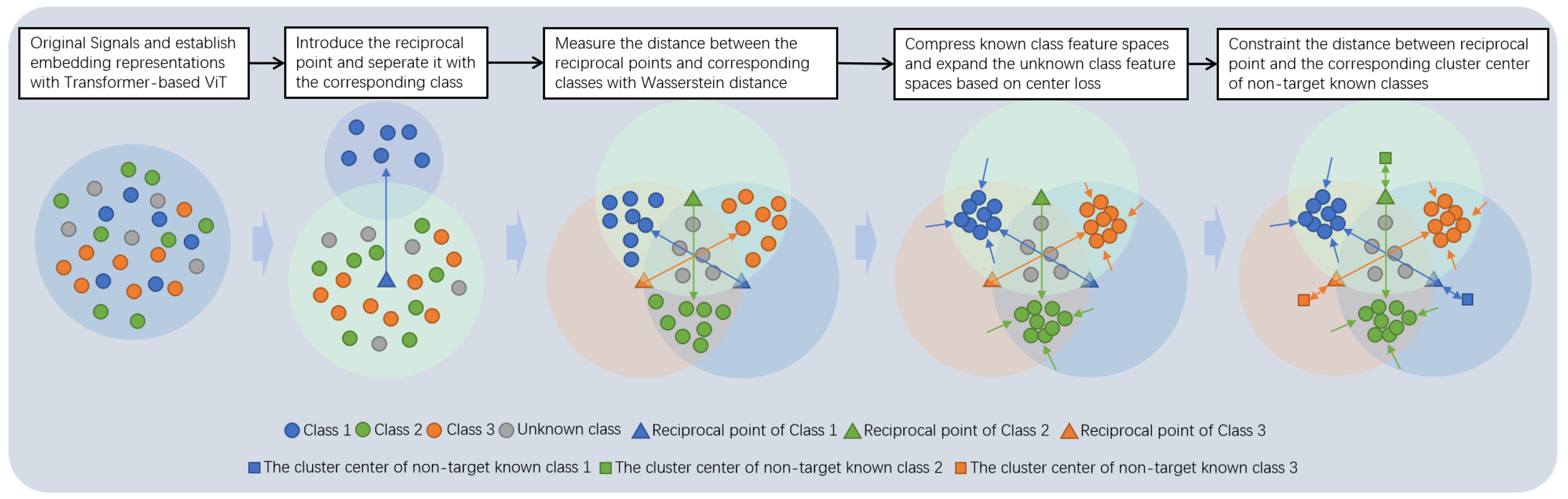
In the present work, we propose an efficient open-set signal recognition algorithm named the open-set signal recognition based on the transformer and Wasserstein distance (${\mathrm{OSSG}}_{TW}$). The algorithm contains three key sub-modules: the signal representation sub-module based on the ViT structure; the set distance metric sub-module based on Wasserstein distance; and the class space compression sub-module based on reciprocal point separation and central loss. In ${\mathrm{OSSG}}_{TW}$, the representing features of the signals are established based on the transformer-based neural networks, i.e., ViT, in order to extract global information about time series-related data. The three sub-modules of ${\mathrm{OSSG}}_{TW}$ are summarized below:

-

The signal representation sub-module: For signal recognition, the signal sequence is typically transformed into time-frequency matrices through energy detection and the short-time fast Fourier transform (FFT). However, although a sequential relationship structure must exist among the columns of the time-frequency matrix, the traditional convolution neural network-based (CNN-based) feature extraction technique lacks the information vision of the global feature. The transformer-based model with the ability to extract the global feature is more suitable for the feature extraction of signal sequences. We employed the transformer-based ViT model as the basic feature extraction scheme to obtain more efficient features of the original signal data.

-

The set distance metric sub-module: The distance of the reciprocal point to the corresponding dataset was determined by combining the Euclidean distance and dot product in the classical ARPL. In order to calculate a better distance to a dataset, the Wasserstein distance could be employed, which is usually used to reflect the distance between distributions (a dataset can be considered as a uniform distribution defined in data samples). Furthermore, the use of the Wasserstein distance could be beneficial in determining the reciprocal point for each category.

-

The class space compression sub-module: In order to realize the recognition of unknown electromagnetic signals by separating the known and unknown electromagnetic signal category feature spaces more accurately, we introduced the center loss to compress the feature space of the known electromagnetic signal target, and expanded the feature space of the unknown electromagnetic signal target based on the well-established feature center of known categories. The feature space range of unknown electromagnetic signal categories can be improved by constraining the inter-class dispersion and intra-class compactness, which could be beneficial in improving the classification performance.

The overall algorithm framework is shown in Figure 1. The details of the above improvements will be discussed in the following sub-sections.

4.1. Signal Representation Sub-Module

The original one-dimensional electromagnetic signal needs to be processed as a fixed time-frequency matrix through energy detection, short-time Fourier transform, and other operations. The short-time Fourier transform usually aims to use a fixed-size window to intercept a small signal sequentially and convert each small signal into a one-dimensional matrix by discrete Fourier transform. Further, all the obtained matrices are spliced into a time-frequency matrix of a well-designed size. The problem of signal recognition can be considered as the task of image classification. From the generation process of a signal sequence as a time-frequency matrix, it can be found that the sequential relationship naturally exists between each column of the matrix. It has been proven that the model with a high recognition rate in the closed set scene has a high positive correlation with the recognition rate in the open set scene. As a result, it would be better to employ some feature extraction models with the global feature extraction ability for open-set scenarios. The transformer [41] was first proposed in natural language processing, which uses the self-attention mechanism to encode global information about the sequence data. The vision transformer, i.e., ViT [42], can be considered the first transformer-based model for computer vision. ViT has a strong global feature extraction ability to extract the features of time-frequency matrices. However, the ViT model network has extreme structural parameters in the training process, requiring data enhancement and regularization techniques to prevent over-fitting with relatively low computational efficiency. In this signal representation sub-module, we employ the lightweight mobile ViT model [43], instead of typical CNN-based models, as the important feature extractor to extract the global features. The mobile ViT combines both the traditional convolution layer and transformer model to learn local and global features, respectively. On the basis of the reduction in parameters to facilitate the training, it has the ability to extract global information.

4.2. Set Distance Metric Sub-Module

Instead of comparing two datasets with respect to the Euclidean metric, we introduced the popular Wasserstein distance. For the given two datasets $\left\{{\mathbf{a}}_i,i=1,\cdots ,m\right\}$ and $\left\{{\mathbf{b}}_j,j=1,\cdots ,n\right\}$, which can be considered as two uniform distributions defined on these two datasets respectively. The corresponding measures can be expressed as:

$$\mathbf{u}=\sum _{i=1}^m\frac{1}{m}{\delta }_{{\mathbf{x}}_i},\mathbf{v}=\sum _{j=1}^n\frac{1}{n}{\delta }_{{\mathbf{y}}_j},$$

where $\delta$ is the function defined in each data sample. The distance between $\left\{{\mathbf{a}}_i,i=1,\cdots ,m\right\}$ and $\left\{{\mathbf{b}}_j,j=1,\cdots ,n\right\}$ can be defined as the Wasserstein distance between $\mathbf{u}$ and $\mathbf{v}$. We first introduced the formulation of the Kantorovich optimal transport problem as follows:

$${\mathrm{L}}_{\mathbf{C}}(\mathbf{u},\mathbf{v})\stackrel{\mathrm{def}.}{=}\underset{\mathbf{P}\in \mathbf{U}(\frac{1}{\mathbf{m}},\frac{1}{\mathbf{n}})}{min}\langle \mathbf{C},\mathbf{P}\rangle \stackrel{\mathrm{def}.}{=}\sum _{i,j}{\mathbf{C}}_{i,j}{\mathbf{P}}_{i,j},$$

(4)

where, the constraint set $\mathbf{U}(\frac{1}{\mathbf{m}},\frac{1}{\mathbf{n}})$ is defined as:

$$\mathbf{U}(\frac{1}{\mathbf{m}},\frac{1}{\mathbf{n}})\stackrel{\mathrm{def}.}{=}\left\{\mathbf{P}\in {\mathbb{R}}_{+}^{n\times m}:\mathbf{P}{\mathbf{1}}_m=\frac{1}{\mathbf{m}},{\mathbf{P}}^{\mathrm{T}}{\mathbf{1}}_n=\frac{1}{\mathbf{n}}\right\},$$

(5)

And matrix $\mathbf{C}$ is the cost matrix while each element ${\mathbf{C}}_{i,j}$ is determined by the corresponding data samples (${\mathbf{a}}_i$ and ${\mathbf{b}}_j$). The Kantorovich optimal transport problem (4) is a linear programming problem with n + m equality constraints. The Wasserstein distance between $\left\{{\mathbf{a}}_i,i=1,\cdots ,m\right\}$ and $\left\{{\mathbf{b}}_j,j=1,\cdots ,n\right\}$ can further be defined as:

$$\mathbf{W}\left(\left\{{\mathbf{a}}_i\right\},\left\{{\mathbf{b}}_j\right\}\right):={\mathrm{L}}_{{\mathbf{D}}^p}(\mathbf{u},\mathbf{v}),$$

(6)

where the distance matrix ${\mathbf{D}}^p$ is used to represent the cost matrix with $0\le p\le 1$. In this paper, the Wasserstein distance is used to improve both the empirical classification risk ${\mathcal{L}}_{known}$ and open space risk ${\mathcal{L}}_o$, i.e.,

$$\left\{\begin{array}{c}p\left(\mathbf{y}=k|\mathbf{x},f,\left\{p^k\right\}\right)=\frac{e^{\gamma \mathbf{W}\left(\left\{\mathbf{x}\right\},p^k\right)}}{{\sum }_{j=1}^{\ell }{e}^{\gamma \mathbf{W}\left(\left\{\mathbf{x}\right\},p^j\right)}}\mathrm{in}{\mathcal{L}}_{known},\hfill \\ {\mathcal{L}}_o\left(\theta ,\left\{p^k\right\},\mathcal{R}\right)=\sum _{k=1}^{\ell }\sum _{{\mathcal{D}}_{train}^{\ne k}\cup {\mathcal{D}}_{\mathcal{U}}}\left\{max\left(\mathbf{W}\left(\left\{\mathbf{x}\right\},p^k\right)-\mathcal{R},0\right)\right\}.\hfill \end{array}\right.$$

(7)

4.3. Class Space Compression Sub-Module

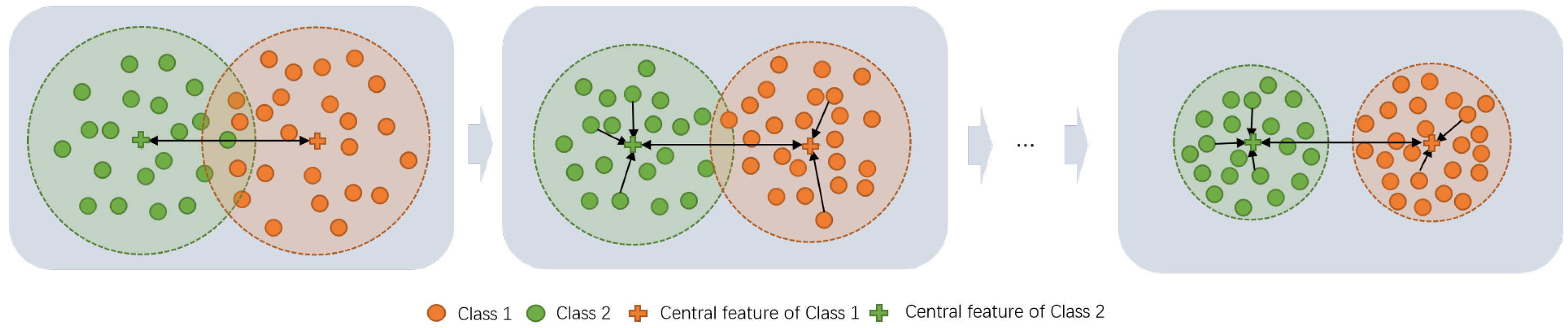
In order to further compress the feature space of known electromagnetic signal targets, the center loss [44] was introduced to optimize our algorithm. The center loss increases the distance between the classes by constraining the inter-class dispersion and intra-class compactness to improve the feature space range of unknown classes. Although it cannot increase the inter-class distance of the class center, the increase in the inter-class edge distance can increase the scope of the unknown class feature space when combined with the definition of reciprocal points to further improve the performance of the method. For each category k, we introduced a central feature ${\mathbf{c}}_k$ to further define the central loss as:

$${\mathcal{L}}_{cen}:=\sum _{k=1}^{\ell }\sum _{{\mathbf{y}}_{\mathbf{x}}=k}{∥h\left(\mathbf{x}\right)-{\mathbf{c}}_k∥}^2,$$

(8)

where $h(·)$ denotes the feature embedding function based on the above signal representation sub-module. The central feature ${\mathbf{c}}_k$ of category k dynamically changes with respect to the signal representation neural network, whose working principle is shown in Figure 2.

However, due to the large amount of data in the training set, the characteristics of each sample are calculated in every iteration, and the central features of each category are updated at the same time, which leads to a large computational overhead and low computational efficiency. Therefore, in the actual training process, the update of the feature center is not based on the entire training set but based on batch samples. In each batch update process, our algorithm calculated the distance between the sample feature and the feature center, and then the calculation result was used to update the feature center. After the establishment of the clustering centers, although the distance between them did not increase, the intra-class space of each target was compressed. In the open set scenario, the feature spaces of the known and unknown electromagnetic signal targets complemented each other in the global space. So, the inclusion of the central loss could also increase the target feature space of the unknown electromagnetic signals and effectively improve the performance of the algorithm.

Furthermore, in order to constrain the convergence direction of reciprocal points, the distance loss between the reciprocal points of each electromagnetic signal category $p^k$ and the cluster center of the non-target and known class targets ${\mathcal{T}}_k$ were introduced, i.e.,

$${\mathcal{L}}_{ac}:={∥{\mathcal{T}}_k-p^k∥}^2.$$

(9)

The overall loss function of our proposed algorithm is expressed as:

$${\mathcal{L}}_{all}\left(\theta ,\left\{p^k\right\},\mathcal{R}\right):={\mathcal{L}}_{known}+\alpha {\mathcal{L}}_o+\beta {\mathcal{L}}_{cen}+\eta {\mathcal{L}}_{ac},$$

(10)

With $\alpha$, $\beta$, and $\eta$ as the related penalty parameters.

4.4. Algorithm Framework

In order to summarize, the overall algorithm, namely the open-set signal recognition based on the transformer and Wasserstein distance (${\mathrm{OSSG}}_{TW}$), can be proposed as:

$$\left\{\begin{array}{c}\left(1\right)\mathrm{Initialize}\mathrm{the}\mathrm{parameters}\theta ,\left\{p^k\right\},\mathcal{R}\mathrm{respectively};\mathrm{set}\hfill \\ \alpha ,\beta ,\eta ,\gamma ,\mathrm{as}\mathrm{the}\mathrm{learning}\mathrm{rate}\mu \mathrm{and}\mathrm{the}\mathrm{iteration}\mathrm{number}t;\hfill \\ \left(2\right)\mathrm{Perform}t\to t+1;\hfill \\ \left(3\right)\mathrm{Calculate}\mathrm{the}\mathrm{loss}\mathrm{by}{\mathcal{L}}_{all}^t\left({\theta }^t,\left\{{\left(p^k\right)}^t\right\},{\mathcal{R}}^t\right);\hfill \\ \left(4\right)\mathrm{Update}\mathrm{the}\mathrm{parameters}\left\{p^k\right\}\mathrm{by}\hfill \\ {\left(p^k\right)}^{t+1}={\left(p^k\right)}^t-\mu \frac{\partial {\mathcal{L}}_{all}^t}{\partial p^k}\left({\theta }^t,\left\{{\left(p^k\right)}^t\right\},{\mathcal{R}}^t\right);\hfill \\ \left(5\right)\mathrm{Update}\mathrm{the}\mathrm{parameters}\mathcal{R}\mathrm{by}\hfill \\ {\mathcal{R}}^{t+1}={\mathcal{R}}^t-\mu \frac{\partial {\mathcal{L}}_{all}^t}{\partial \mathcal{R}}\left({\theta }^t,\left\{{\left(p^k\right)}^t\right\},{\mathcal{R}}^t\right);\hfill \\ \left(6\right)\mathrm{Update}\mathrm{the}\mathrm{parameters}\theta \mathrm{by}\hfill \\ {\theta }^{t+1}={\theta }^t-\mu \frac{\partial {\mathcal{L}}_{all}^t}{\partial \theta }\left({\theta }^t,\left\{{\left(p^k\right)}^t\right\},{\mathcal{R}}^t\right).\hfill \end{array}\right.$$

5. Experiments

In this section, experimental verification with two collected electromagnetic signal datasets is conducted, and four state-of-the-art open-set signal recognition methods are compared according to some typical evaluation metrics.

5.1. Datasets

Two electromagnetic signal datasets are considered in this paper, i.e., Mobile dataset and Radio dataset.

The mobile dataset contained electromagnetic signals from 10 mobile phones, including three Glory-10 mobile phones, one Huawei-P9 mobile phone, three Apple-6s mobile phones, one Meizu-X8 mobile phone, and two OPPO-R11 mobile phones. The Radio dataset was taken from the electromagnetic signals collected from 10 radio stations, including three MESHs_1UE radio stations, three MESHs_2UE large radio stations, three round small radio stations, and one round large radio station. After implementing the filter, energy detection, slice, and STFT operations on the original signals, a series of $224\times 224$ labeled complex matrices were generated. By separating the real and imaginary parts, the time-frequency matrix samples of the dimension of $2\times 224\times 224$ could be established. Finally, the dataset with the signal samples of the $3\times 224\times 224$ dimension could be constructed with some splicing operations (the corresponding mean values of the first and second dimensions were set to be the third dimension). In order to reflect universality, we conducted five experiments for each algorithm. Each experiment randomly selected six out of the ten targets as the known electromagnetic signals, such as targets (labeled 0–5), and the remaining four targets as the unknown electromagnetic signals, such as targets (labeled 6).

5.2. Evaluation Metric

In order to more comprehensively evaluate the performance of the method, we evaluated all the algorithms on the AUC, Accuracy and PRE indicators for both the known and unknown signals.

AUC: The AUC index indicates the probability of the model scores, where the randomly selected positive category is higher than the negative category. The AUC index was obtained by calculating the area under the ROC curve, which is calculated by two parameters (namely, TPR and FPR). The ROC curve is established with FPR as the X-axis and TPR as the Y-axis, which can be expressed as:

$$\begin{array}{c}\hfill \mathit{TPR}:=\frac{TP}{TP+FN},\mathit{FPR}:=\frac{FP}{FP+TN}.\end{array}$$

(11)

Accuracy: The basic accuracy index refers to the ratio of the number of correctly predicted samples over the total number of predicted samples, which can be expressed as:

$$\mathit{Accuracy}:=\frac{{\sum }_i\left(T{P}_i+T{N}_i\right)}{{\sum }_i\left(T{P}_i+T{N}_i+F{P}_i+F{N}_i\right)}.$$

(12)

PRE: The PRE index refers to the ratio of the number of positive samples that are predicted correctly to the number of all positive samples predicted. Different from the accuracy index, the PRE index focuses only on the part predicted as the positive samples, which can be expressed as:

$$\mathit{PRE}:=\frac{{\sum }_{i}T{P}_i}{{\sum }_i\left(T{P}_i+F{P}_i\right)}.$$

(13)

In order to reflect the difference between the identification performances of the open-set recognition methods, all the experimental indicators were calculated for both the known and unknown categories.

5.3. Baseline Algorithms

Many state-of-the-art open-set recognition methods are compared below, including OpenMax [21], G-OpenMax [38], CROSR [23], ARPL [26], and SARPL [26]. Furthermore, we compared our proposed algorithm with some ablation versions in order to show the efficiency of the introduced sub-modules. Those methods are briefly introduced below:

(1)

OpenMax [21]: A typical discriminative model-based method with OpenMax layer;

(2)

G-OpenMax [38]: A generative model-based method extended from OpenMax, which employs the conditional generation countermeasure network (GAN) to generate unknown class samples;

(3)

CROSR [23]: An improved version of OpenMax, which is obtained through reconstructing samples and encoding more original samples to improve the performance in open set scenarios;

(4)

ARPL [26]: The reciprocal points are introduced to separate the feature spaces of the known and unknown classes, and the classification is determined by a threshold method.

(5)

SARPL [26]: Based on the classical ARPL method, we introduced the proposed ${\mathcal{L}}_{ac}$ loss function to constrain the convergence direction of the reciprocal points. This SARPL can be considered as an ablation version of our proposed algorithm ${\mathrm{OSSG}}_{TW}$ without the ViT, Wasserstein distance, and central loss techniques.

(6)

Ablation versions: ${\mathrm{OSSG}}_{TW}$(w/o CL) and ${\mathrm{OSSG}}_{TW}$(w/o W/CL) are the versions without central loss, and without both Wasserstein distance and central loss, respectively.

5.4. Comparisons

Table 1. The results of the phones.

Method	Accuracy (%)		PRE (%)		AUC (%)
	Known	Unknown	Known	Unknown	Knonw	Unknow
OpenMax	82.62 (±2.11)	86.31 (±1.38)	81.70 (±2.91)	85.07 (±2.53)	89.57 (±1.97)	89.79 (±3.10)
G-OpenMax	84.84 (±3.12)	87.98 (±2.53)	83.29 (±2.56)	84.74 (±1.01)	90.90 (±2.47)	90.84 (±2.01)
CROSR	87.29 (±2.91)	90.62 (±1.76)	88.01 (±2.32)	89.62 (±2.77)	92.37 (±2.21)	92.18 (±1.34)
ARPL	88.64 (±2.83)	91.70 (±2.14)	89.38 (±2.23)	91.21 (±1.65)	93.18 (±1.92)	91.41 (±1.71)
SARPL	88.94 (±2.16)	92.18 (±2.05)	89.55 (±1.93)	91.98 (±1.44)	93.36 (±2.19)	92.98 (±1.75)
${\mathrm{OSSG}}_{TW}$ (w/o W/CL)	91.58 (±1.34)	93.01 (±1.28)	92.93 (±1.19)	92.29 (±1.12)	94.75 (±1.23)	93.12 (±1.38)
${\mathrm{OSSG}}_{TW}$ (w/o CL)	92.01 (±2.24)	93.29 (±1.23)	92.45 (±1.02)	92.77 (±1.43)	95.21 (±1.38)	93.53 (±1.48)
${\mathrm{OSSG}}_{TW}$	93.82 (±1.94)	94.83 (±1.73)	94.21 (±1.12)	94.62 (±2.26)	96.44 (±1.65)	95.32 (±1.76)

,

Table 2. The results of the radios.

Method	Accuracy (%)		PRE (%)		AUC (%)
	Known	Unknown	Known	Unknown	Known	Unknow
OpenMax	78.52 (±1.38)	80.16 (±1.11)	78.24 (±1.62)	77.84 (±1.34)	87.11 (±1.31)	81.84 (±1.34)
G-OpenMax	80.34 (±2.10)	81.90 (±2.81)	82.21 (±3.31)	78.56 (±2.46)	88.20 (±2.55)	83.48 (±1.34)
CROSR	81.35 (±1.70)	85.10 (±1.42)	81.98 (±3.13)	83.92 (±3.39)	88.81 (±1.09)	86.02 (±2.65)
ARPL	82.83 (±2.40)	88.09 (±2.83)	81.99 (±1.25)	87.04 (±2.13)	89.70 (±1.19)	87.56 (±1.06)
SARPL	83.54 (±1.74)	88.84 (±1.11)	82.98 (±2.37)	87.72 (±1.19)	90.13 (±2.98)	88.40 (±1.41)
${\mathrm{OSSG}}_{TW}$ (w/o W/CL)	84.78 (±1.81)	90.39 (±1.11)	84.82 (±1.39)	89.82 (±1.94)	90.89 (±2.02)	90.03 (±1.49)
${\mathrm{OSSG}}_{TW}$ (w/o CL)	85.15 (±2.03)	91.02 (±1.39)	85.92 (±1.92)	90.23 (±1.58)	91.28 (±1.30)	90.37 (±1.58)
${\mathrm{OSSG}}_{TW}$	86.24 (±1.13)	92.62 (±1.27)	86.25 (±1.18)	91.63 (±1.89)	91.74 (±1.39)	92.93 (±2.96)

and

Table 3. The definition of some fundamental metrics.

Actual	Predicted
	Positive	Negative
Positive	$TP$	$FN$
Negative	$FP$	$TN$

contain the main results on the mobile and radio datasets, respectively. It was found that the proposed ${\mathrm{OSSG}}_{TW}$ significantly improved the results of all the indicators on both the mobile and radio datasets. Compared with the classical APRL algorithm, the accuracy indicator on the known classes was improved by 5.18%, while the AUC indicator was improved by 3.26%. As for the unknown categories, the accuracy index was increased by 3.13%. The most significant improvements included the increase of up to 4.26% in the PRE index and up to 5.37% in the AUC index with respect to the known and unknown datasets, respectively. The proposed ${\mathrm{OSSG}}_{TW}$ algorithm was compared with some ablation versions, which also shows the efficiency of the proposed three basic sub-modules. It was found that the effect of using the ViT model to extract the features and employing the center loss to reduce the distance within the target feature classes produced a 1–2% improvement in each index, while the Wasserstein distance produced less than a 1% improvement due to the overall effect.

6. Conclusions

In this work, we proposed an efficient open-set signal recognition algorithm called ${\mathrm{OSSG}}_{TW}$, which contains three key sub-modules: the signal representation sub-module based on the ViT structure, the set distance metric sub-module based on Wasserstein distance, and the class space compression sub-module based on reciprocal point separation and central loss. Numerical experiments on different open-set signal recognition tasks show that the proposed algorithm can significantly improve the recognition efficiency of both known and unknown categories.

References

- O’Shea, T.J.; Corgan, J.; Clancy, T.C. Unsupervised representation learning of structured radio communication signals. In Proceedings of the SPLINE, Aalborg, Denmark, 6–8 July 2016. [Google Scholar]
- O’Shea, T.J.; Roy, T.; Clancy, T.C. Over-the-Air Deep Learning Based Radio Signal Classification. IEEE J. Sel. Top. Signal Process. 2018, 12, 168–179. [Google Scholar] [CrossRef]
- Dong, Y.; Jiang, X.; Zhou, H.; Lin, Y.; Shi, Q. SR2CNN: Zero-Shot Learning for Signal Recognition. IEEE Tran. Signal Process. 2021, 69, 2316–2329. [Google Scholar] [CrossRef]
- Dong, Y.; Jiang, X.; Cheng, L.; Shi, Q. SSRCNN: A Semi-Supervised Learning Framework for Signal Recognition. IEEE Trans. Cogn. Commun. Netw. 2021, 7, 780–789. [Google Scholar] [CrossRef]
- Khan, H.; Xiao, B.; Li, W.; Muhammad, N. Recent advancement in haze removal approaches. Multimed. Syst. 2022, 28, 687–710. [Google Scholar] [CrossRef]
- Batool, R.; Bibi, N.; Muhammad, N.; Alhazmi, S. Detection of Primary User Emulation Attack Using the Differential Evolution Algorithm in Cognitive Radio Networks. Appl. Sci. 2022, 13, 571. [Google Scholar] [CrossRef]
- Geng, C.; Huang, S.; Chen, S. Recent Advances in Open Set Recognition: A Survey. IEEE Trans. Pattern Anal. Mach. Intell. 2021, 43, 3614–3631. [Google Scholar] [CrossRef]
- Scheirer, W.J.; de Rezende Rocha, A.; Sapkota, A.; Boult, T.E. Toward Open Set Recognition. IEEE Trans. Pattern Anal. Mach. Intell. 2013, 35, 1757–1772. [Google Scholar] [CrossRef]
- Scheirer, W.J.; Jain, L.P.; Boult, T.E. Probability Models for Open Set Recognition. IEEE Trans. Pattern Anal. Mach. Intell. 2014, 36, 2317–2324. [Google Scholar] [CrossRef]
- Jain, L.P.; Scheirer, W.J.; Boult, T.E. Multi-class Open Set Recognition Using Probability of Inclusion. In Proceedings of the ECCV, Zurich, Switzerland, 6–12 September 2014. [Google Scholar]
- Sun, X.; Li, X.; Ren, K.; Song, J.; Xu, Z.; Chen, J. Rethinking compact abating probability modeling for open set recognition problem in Cyber-physical systems. J. Syst. Archit. 2019, 101, 101660. [Google Scholar] [CrossRef]
- Scherreik, M.D.; Rigling, B.D. Open set recognition for automatic target classification with rejection. IEEE Trans. Aerosp. Electr. Syst. 2016, 52, 632–642. [Google Scholar] [CrossRef]
- Cevikalp, H. Best Fitting Hyperplanes for Classification. IEEE Trans. Pattern Anal. Mach. Intell. 2017, 39, 1076–1088. [Google Scholar] [CrossRef]
- Cevikalp, H.; Triggs, B. Polyhedral Conic Classifiers for Visual Object Detection and Classification. In Proceedings of the CVPR, Honolulu, HI, USA, 21–26 July 2017. [Google Scholar]
- Zhang, H.; Patel, V.M. Sparse Representation-Based Open Set Recognition. IEEE Trans. Pattern Anal. Mach. Intell. 2017, 39, 1690–1696. [Google Scholar] [CrossRef]
- Júnior, P.R.M.; de Souza, R.M.; de Oliveira Werneck, R.; Stein, B.V.; Pazinato, D.V.; de Almeida, W.R.; Penatti, O.A.B.; da Silva Torres, R.; Rocha, A. Nearest neighbors distance ratio open-set classifier. Mach. Learn. 2017, 106, 359–386. [Google Scholar] [CrossRef]
- Vareto, R.H.; Silva, S.; de Oliveira Costa, F.; Schwartz, W.R. Towards open-set face recognition using hashing functions. In Proceedings of the IJCB, Denver, CO, USA, 1–4 October 2017. [Google Scholar]
- Rudd, E.M.; Jain, L.P.; Scheirer, W.J.; Boult, T.E. The Extreme Value Machine. IEEE Trans. Pattern Anal. Mach. Intell. 2018, 40, 762–768. [Google Scholar] [CrossRef]
- Bendale, A.; Boult, T.E. Towards Open Set Deep Networks. In Proceedings of the CVPR, Las Vegas, NV, USA, 26 June–1 July 2016. [Google Scholar]
- Prakhya, S.; Venkataram, V.; Kalita, J. Open Set Text Classification Using CNNs. In Proceedings of the ICON, Antalya, Turkey, 18–21 December 2017. [Google Scholar]
- Shu, L.; Xu, H.; Liu, B. DOC: Deep Open Classification of Text Documents. In Proceedings of the EMNLP, Copenhagen, Denmark, 7–11 September 2017. [Google Scholar]
- de O. Cardoso, D.; Gama, J.; França, F.M.G. Weightless neural networks for open set recognition. Mach. Learn. 2017, 106, 1547–1567. [Google Scholar]
- Yoshihashi, R.; Shao, W.; Kawakami, R.; You, S.; Iida, M.; Naemura, T. Classification-Reconstruction Learning for Open-Set Recognition. In Proceedings of the CVPR, Long Beach, CA, USA, 16–20 June 2019. [Google Scholar]
- Oza, P.; Patel, V.M. C2AE: Class Conditioned Auto-Encoder for Open-Set Recognition. In Proceedings of the CVPR, Long Beach, CA, USA, 16–20 June 2019. [Google Scholar]
- Hassen, M.; Chan, P.K. Learning a Neural-network-based Representation for Open Set Recognition. In Proceedings of the SDM, Split, Croatia, 24–26 June 2020. [Google Scholar]
- Chen, G.; Peng, P.; Wang, X.; Tian, Y. Adversarial Reciprocal Points Learning for Open Set Recognition. IEEE Trans. Pattern Anal. Mach. Intell. 2022, 44, 8065–8081. [Google Scholar] [CrossRef]
- Mahdavi, A.; Carvalho, M. A Survey on Open Set Recognition. In Proceedings of the AIKE, Laguna Hills, CA, USA, 1–3 December 2021. [Google Scholar]
- O’Shea, T.J.; Corgan, J.; Clancy, T.C. Convolutional Radio Modulation Recognition Networks. In Proceedings of the EANN, Aberdeen, UK, 2–5 September 2016. [Google Scholar]
- Peng, S.; Jiang, H.; Wang, H.; Alwageed, H.; Zhou, Y.; Sebdani, M.M.; Yao, Y. Modulation Classification Based on Signal Constellation Diagrams and Deep Learning. IEEE Trans. Neural Netw. Learn. Syst. 2019, 30, 718–727. [Google Scholar] [CrossRef]
- Zheng, S.; Chen, S.; Yang, L.; Zhu, J.; Luo, Z.; Hu, J.; Yang, X. Big Data Processing Architecture for Radio Signals Empowered by Deep Learning: Concept, Experiment, Applications and Challenges. IEEE Access 2018, 6, 55907–55922. [Google Scholar] [CrossRef]
- Flowers, B.; Buehrer, R.M.; Headley, W.C. Evaluating Adversarial Evasion Attacks in the Context of Wireless Communications. IEEE Trans. Inf. Forensics Secur. 2020, 15, 1102–1113. [Google Scholar] [CrossRef]
- Duan, S.; Chen, K.; Yu, X.; Qian, M. Automatic Multicarrier Waveform Classification via PCA and Convolutional Neural Networks. IEEE Access 2018, 6, 51365–51373. [Google Scholar] [CrossRef]
- Wong, L.J.; Headley, W.C.; Michaels, A.J. Specific Emitter Identification Using Convolutional Neural Network-Based IQ Imbalance Estimators. IEEE Access 2019, 7, 33544–33555. [Google Scholar] [CrossRef]
- Huang, S.; Chai, L.; Li, Z.; Zhang, D.; Yao, Y.; Zhang, Y.; Feng, Z. Automatic Modulation Classification Using Compressive Convolutional Neural Network. IEEE Access 2019, 7, 79636–79643. [Google Scholar] [CrossRef]
- Dörner, S.; Cammerer, S.; Hoydis, J.; ten Brink, S. Deep Learning Based Communication Over the Air. IEEE J. Sel. Top. Signal Process. 2018, 12, 132–143. [Google Scholar] [CrossRef] [Green Version]
- Kardan, N.; Stanley, K.O. Mitigating fooling with competitive overcomplete output layer neural networks. In Proceedings of the IJCNN, Anchorage, AK, USA, 14–19 May 2017. [Google Scholar]
- Neal, L.; Olson, M.; Fern, X.; Wong, W.K.; Li, F. Open Set Learning with Counterfactual Images. In Proceedings of the ECCV, Munich, Germany, 8–14 September 2018. [Google Scholar]
- Ge, Z.; Demyanov, S.; Garnavi, R. Generative OpenMax for Multi-Class Open Set Classification. In Proceedings of the BMVC, London, UK, 4–7 September 2017. [Google Scholar]
- Yu, Y.; Qu, W.Y.; Li, N.; Guo, Z. Open-category classification by adversarial sample generation. In Proceedings of the IJCAI, Melbourne, Australia, 19–25 August 2017. [Google Scholar]
- Yue, Z.; Wang, T.; Zhang, H.; Sun, Q.; Hua, X.S. Counterfactual Zero-Shot and Open-Set Visual Recognition. In Proceedings of the CVPR, Online, 19–25 June 2021. [Google Scholar]
- Vaswani, A.; Shazeer, N.; Parmar, N.; Uszkoreit, J.; Jones, L.; Gomez, A.N.; Kaiser, L.; Polosukhin, I. Attention is All you Need. In Proceedings of the NeurIPS, Long Beach, CA, USA, 4–9 December 2017; pp. 5998–6008. [Google Scholar]
- Dosovitskiy, A.; Beyer, L.; Kolesnikov, A.; Weissenborn, D.; Zhai, X.; Unterthiner, T.; Dehghani, M.; Minderer, M.; Heigold, G.; Gelly, S.; et al. An Image is Worth 16x16 Words: Transformers for Image Recognition at Scale. In Proceedings of the ICLR, Online, 3–7 May 2021. [Google Scholar]
- Mehta, S.; Rastegari, M. MobileViT: Light-weight, General-purpose, and Mobile-friendly Vision Transformer. In Proceedings of the ICLR, Online, 25–29 April 2022. [Google Scholar]
- Wen, Y.; Zhang, K.; Li, Z.; Qiao, Y. A discriminative feature learning approach for deep face recognition. In Proceedings of the European Conference on Computer Vision, Amsterdam, The Netherlands, 11–14 October 2016; pp. 499–515. [Google Scholar]
Figure 1.
Main algorithm framework containing three key sub-modules: the signal representation sub-module based on tansformer-based ViT structure; the set distance metric sub-module based on Wasserstein distance; abd the class space compression sub-module based on reciprocal point separation and central loss.
Figure 2.
The principles of the proposed center loss and the central feature. The center loss drives the embedding features of each category to accumulate to the corresponding central feature .