
Determination of Harmonic Parameters in Pathological Voices—Efficient Algorithm
by
 ,
,
Joana Filipa Teixeira Fernandes
1,2,
Diamantino Freitas
2,
Arnaldo Candido Junior
3 and
João Paulo Teixeira
1,4,5,*
1
Research Centre in Digitalization and Intelligent Robotics (CeDRI), Instituto Politécnico de Bragança, Campus de Santa Apolónia, 5300-253 Bragança, Portugal
2
Faculty of Engineering, University of Porto (FEUP), 4200-465 Porto, Portugal
3
Institute of Biosciences, Language and Physical Sciences, São Paulo State University, São José do Rio Preto 15054-000, Brazil
4
Laboratório para a Sustentabilidade e Tecnologia em Regiões de Montanha (SusTEC), Instituto Politécnico de Bragança, Campus de Santa Apolónia, 5300-253 Bragança, Portugal
5
Applied Management Research Unit (UNIAG)—Instituto Politécnico de Bragança, Campus de Santa Apolónia, 5300-253 Bragança, Portugal
*
Author to whom correspondence should be addressed.
Appl. Sci. 2023, 13(4), 2333; https://doi.org/10.3390/app13042333
Submission received: 22 December 2022
/
Revised: 7 February 2023
/
Accepted: 9 February 2023
/
Published: 11 February 2023
(This article belongs to the Special Issue Current Trends and Future Directions in Voice Acoustics Measurement)
Abstract
:Featured Application
The paper describes a low-complexity/efficient algorithm to determine the short-term Autocorrelation, HNR, and NHR in sustained vowel audios, to be used in stand-alone devices with low computational power. These parameters can be used as input features of a smart medical decision support system for speech pathology diagnosis.
Abstract
The harmonic parameters Autocorrelation, Harmonic to Noise Ratio (HNR), and Noise to Harmonic Ratio are related to vocal quality, providing alternative measures of the harmonic energy of a speech signal. They will be used as input resources for an intelligent medical decision support system for the diagnosis of speech pathology. An efficient algorithm is important when implementing it on low-power devices. This article presents an algorithm that determines these parameters by optimizing the window type and length. The method used comparatively analyzes the values of the algorithm, with different combinations of window and size and a reference value. Hamming, Hanning, and Blackman windows with lengths of 3, 6, 12, and 24 glottal cycles and various sampling frequencies were investigated. As a result, we present an efficient algorithm that determines the parameters using the Hanning window with a length of six glottal cycles. The mean difference of Autocorrelation is less than 0.004, and that of HNR is less than 0.42 dB. In conclusion, this algorithm allows extraction of the parameters close to the reference values. In Autocorrelation, there are no significant effects of sampling frequency. However, it should be used cautiously for HNR with lower sampling rates.
1. Introduction
A disturbance in the voice has profound implications for a person’s social and professional life. In patients with progressive pathologies, it is essential to have access to a rapid diagnosis to promote better treatment and prognosis [1].
Some tests can be performed to detect voice pathologies, such as laryngoscopy, endoscopy, or stroboscopic exams. However, they are more or less invasive tests, at least from the patient’s point of view, and they cause discomfort [2].
Electroglottography (EGG) is a non-invasive technique that allows measuring the vibration of the vocal folds during speech and singing [3]. It can provide important information about the function of the vocal folds and phonation, as well as the durations of glottic closure and opening patterns [4]. It can be combined with other diagnostic techniques, such as videostroboscopy, for a more comprehensive evaluation of the vocal folds [5]. This technique is helpful in voice therapy, as it allows real-time feedback and assessment of the patient’s progress with the treatment being performed [6]. However, this technique has some limitations, such as sensitivity to skin conductance changes and difficulty obtaining clear signals in some individuals [7]. This technique is not used in this work since it is necessary to use an electroglottograph, which is not always available.
Acoustic analysis is a non-invasive technique that allows the determination of the individual’s voice quality and allows a pre-diagnosis, avoiding several invasive tests. It is a technique that can be used to diagnose and study vocal pathologies as it will enable measuring the acoustic signal properties of recorded speech or sustained vowels [8,9,10].
Several acoustic parameters can be used in the evaluation and classification of vocal pathologies, such as Peak Slope (PS), a ratio of the first harmonic to the second harmonic energy (H1/H2), Normalized Amplitude Quotient (NAQ), Cepstral Peak Prominence (CPP), Mel-Frequency Cepstral Coefficients (MFCCs), Autocorrelation, Harmonic to Noise Ratio (HNR), and Noise to Harmonic Ratio (NHR) [11,12,13].
The parameters Autocorrelation, Harmonic to Noise Ratio, and Noise to Harmonic Ratio are used by several authors as features to describe voice quality in assessment tools for voice pathologies [14,15,16,17,18,19].
Concerning the pathological voices classification tools, several models have been used. Kolhatkar et al., 2016 [14], used the k-Nearest Neighbors (k-NN) algorithm to identify and classify pathological voices from normophonic voices. Ankışhan and İnam, 2021 [17], used a Convolutional Neural Network (CNN) and Long Short-Term Memory (LSTM) recurrent neural network model in their internal structure to classify pathological and normophonic voices. Guedes et al., 2019 [20], used LSTM and CNN to classify four voice disturbance classes, dysphonia, chronic laryngitis, vocal cord paralysis, and normophonic voices. In previous work, Oliveira et al., in 2020 [21] used several parameters, including Autocorrelation, HNR, and NHR, and performed a statistical analysis using the boxplot tool to compare several pathologies. The authors have identified three clusters of pathologies. Guedes et al., 2018 [22], intended to classify chronic laryngitis and normophonic subjects. They used LSTM and Feedforward Artificial Neural Network (ANN) classifiers and Autocorrelation, relative jitter, and relative shimmer input parameters. In this binary classification, an accuracy of 99% was achieved. In Teixeira et al., 2018 [23], several combinations of input features were experimented with, including HNR, using a Support Vector Machine (SVM) classifier to classify between pathological (a set of three pathologies) and normophonic voices. The author’s best accuracy was 71%.
Several authors have developed pathological voice identification systems, that allow the identification of some pathologies using different parameters. However, there are no devices that make the diagnosis automatically, or that allow the identification of pathologies automatically.
This manuscript contributes with an efficient algorithm for determination of autocorrelation, HNR, and NHR in order to develop devices using efficient algorithms to support the diagnosis of pathologies. Concerning the determination of harmonic parameters for voice analysis purposes, Bielamowicz et al. in 1996 [24], compared fundamental frequency (fo), jitter, shimmer and harmonics—or signal-to-noise ratio (HNR) measures made by commercially available acoustical analysis programs (CSpeech—Computer software working on DOS—Wisconsin, DC, USA, Computerized Speech Laboratory—PENTAX Medical—Hoya, Japan, SoundScope—Microsoft, and hand marking)—using a set of dysphonic voices. Measurements of HNR were demonstrated to receive a poor rank-order correlation between programs. Correlations between 0.4 and 0.6 resulted from the two-by-two comparison of the referred programs. The average HNR Hand marked with 21.31 dB received an average HNR of 8.58, 14.34, and 18.48 dB. This result showed very low consistency between commercial systems software to determine HNR.
In signal processing, the Autocorrelation of a discrete time signal (or a time series) is the correlation of the signal with a lagged copy of itself as a function of the lag. The autocorrelation has maxima at lags equal to multiples of the fundamental period (T0 = 1/fo). The value considered in this work for the Autocorrelation parameter, in the context of speech signals, is the amplitude of the first peak after zero delays. Since the algorithm will be applied to quasi-periodic signals (voiced speech produced during the utterance of a vowel), this peak corresponds to the period of the quasi-periodic signal. It provides the identification of similar speech waveforms repeated throughout the signal. For the normalized Autocorrelation, this parameter can vary between 0 and 1, for white noise signals and periodic signals (harmonic component only), respectively. The Autocorrelation is very close to 1 (higher than 0.990) for normophonic voices and lower for dysphonic voices because normophonic voices uttering a vowel signal have mainly harmonic components (periodic) and very low noisy components (aperiodic). In contrast, dysphonic voices (depending on the pathology) tend to have lower harmonic components and higher aperiodic or noisy components.
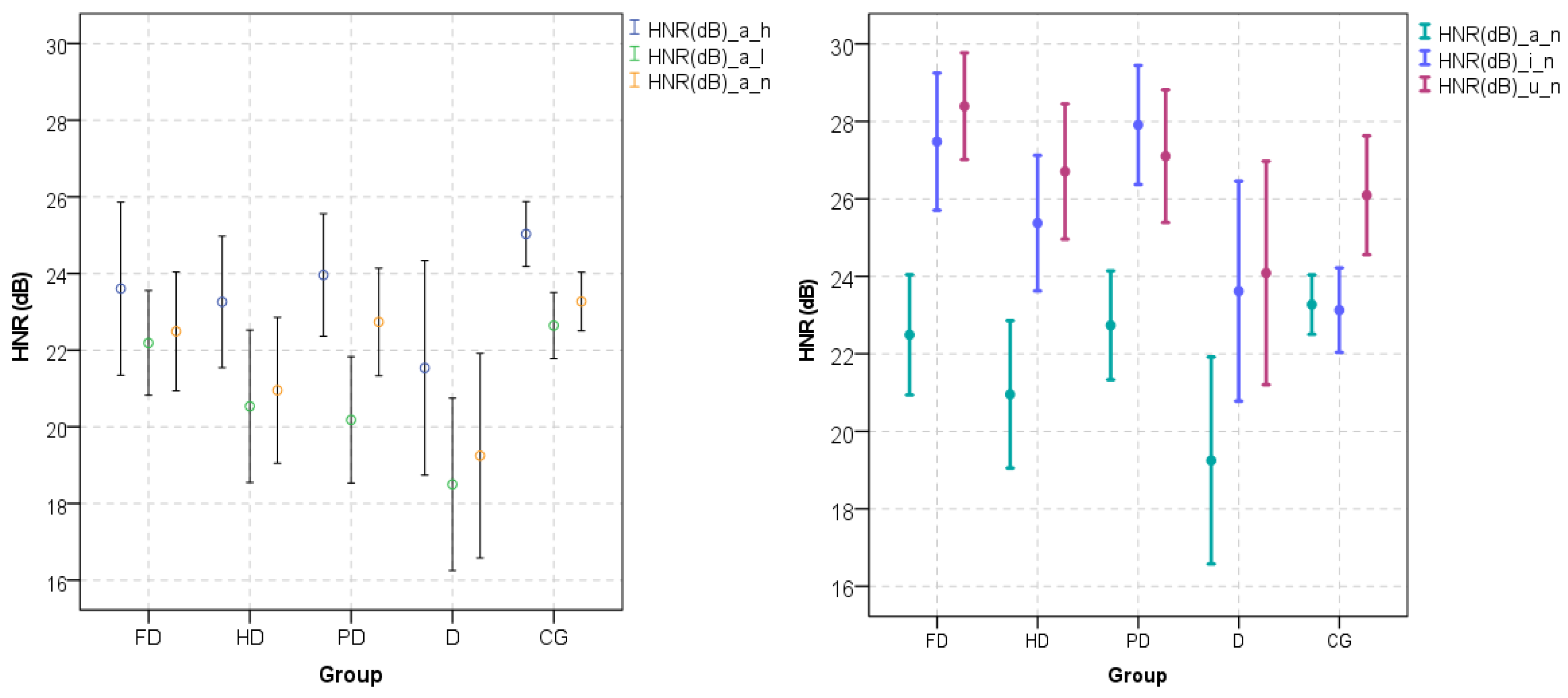
The HNR is a parameter in which the relationship between the harmonic and noisy components of a voiced speech segment indicates the general voice quality of the speech signal. The cyclic opening and closing of the vocal folds produce the harmonic components. The higher the HNR of a voiced signal, the higher the harmonic components, denoting normophonic behavior. It is common to find an HNR of over 20 dB in normophonic voices. There is no threshold value between normophonic and pathological voices, but there is a tendency for normophonic voices to have higher values and lower variance for HNR for the vowel /a/ [25,26]. However, for vowel /u/, there is no statistical significance for different HNR between control and dysphonic voices, as shown in Figure 1 (right-hand side). As can be seen in Figure 1 (left-hand side), Teixeira and Fernandes [25] showed statistically significant higher values of HNR for the higher tone (higher fo) of the /a/ vowel than for normal and lower tones (lower fo). The same authors showed (Figure 1) statistically significant higher values of HNR for the vowel /u/ than for the vowel /a/. This difference evidences the dependency of the HNR on the sound and its structure concerning the frequency and energy of its formants.
In the literature, there are basically three methods for determining the HNR. These methods are based on the time, spectral, and cepstral domains. All methods are applied to a short-time signal window.
The algorithm proposed here is based on the time domain, and the results are compared with another method based on the time domain, as is the case of Boersma’s algorithm [27]. Boersma’s algorithm uses the second peak of the normalized Autocorrelation to determine the HNR. The differences are detailed in Section 2.4.
Algorithms based on spectral components separate the signal spectrum into harmonic and noise regions, considering peaks as the center of harmonic regions and valleys as noise regions. Yegnanarayana and Darsinos, 1995 [28], is based on the iterative reconstruction of the signal. Initially, using Linear Predictive (LP) analysis, speech is separated into approximate excitation and filter components. Next, noise frequency regions and deterministic excitation components are identified using the cepstrum. Two excitation components are reconstructed using an iterative algorithm. Finally, the deterministic and stochastic components of the excitation are obtained by combining the reconstructed data frames using an overlay and addition procedure. These components are passed through the time-varying all-pole filter to get the speech signal components. In this method, it is considered that the spectral peaks correspond to the information of the harmonic component, and the valleys correspond to the noise. Additionally, in 2009, Sousa [29] proposed a method where initially the signal is segmented into frames, and then a sine wave is applied. The harmonic component is estimated from the Odd Discrete Fourier Transform (ODFT) of the signal by extracting each harmonic’s frequency, magnitude and phase. In the ODFT domain, the parameters of the harmonic structure are easily measured and are not significantly affected by noise. These parameters are used to synthesize the harmonic structure in the ODFT domain. The harmonic component is subtracted from the complete signal, producing the noise component estimate. Based on a comparison with other methods, the author mentioned that this algorithm is more suitable for high fo signals (female voices). Deliyski in 1993 [30], proposed an algorithm based on spectral components. However, this algorithm seems to have some difficulties in determining the peaks and valleys, which sometimes arise when there is a peak with a low amplitude followed by one with a high amplitude.
Algorithms based on cepstral analysis consider that the harmonic components are represented by the rahmonic peaks (cepstrum peaks), and the noise components are concentrated in the low quefrencies. The segmentation of zones with harmonic or noise components is based on short-pass or comb lifters, adequately dimensioned. These lifters (filters in the cepstral domain) estimate the noise’s spectral baseline, which allows the determination of the HNR value [31].
The NHR parameter quantifies the relationship between the aperiodic component (noise) and the periodic component (harmonic part) [32]. This parameter is rarely used because it is directly related to the Autocorrelation, as described below. NHR has very low values for normophonic voices and can be slightly higher for some pathological voices.
The development of an algorithm that allows for determining these parameters is presented. As a reference, version 6.0.33 Praat software’s output values for the same acoustic signals are used for comparison. This software is generally used by the scientific community and speech therapeutic professionals. It should be mentioned that the Praat algorithm has a higher complexity level than the one proposed in this manuscript because it determines several candidates for the peaks of the Autocorrelation [27]. The Praat algorithm is designed to deal with any speech segment, while the proposed algorithm is intended to deal only with voiced speech segments.
The focus for developing an alternative algorithm is to create low-complexity algorithms independent of Praat, to be used in a support system for diagnosing vocal pathologies.
The present paper describes the low-complexity algorithm to determine the short-term Autocorrelation, HNR, and NHR of sustained vowel audios, to be used in stand-alone devices with low computational power. These parameters can be used as input features of a smart medical decision support system for speech pathology diagnosis.
The methodology compares the values determined by the algorithm with the values taken as a reference defined by the general purpose Praat software. Different window shapes and lengths were experimented with. In addition, the sensitivity of the algorithm with sampling frequency was measured.
This article is organized as follows: Section 2 describes the pathologies and the database used, the number of subjects for the study, and the foundations of the parameter determination: Autocorrelation, HNR, and NHR. This section also describes the low-complexity algorithm developed to determine the parameters. Section 3 presents the results obtained with different windows and window lengths, the results with lower sampling frequencies, and a preliminary discussion. Finally, Section 4 presents the discussion and final conclusions.
2. Materials and Methods
This section presents the groups of voice disorders, the voice database used, and the theoretical framework for the determination of Autocorrelation, HNR, and NHR.
The justification for this methodology is based on the need for an efficient algorithm to use in hospital devices and for tracking vocal pathologies.
The automatic acquisition and analysis of speech signals in the diagnostic aid device are performed using the platform under development [33]. It performs the acquisition and pre-processing to identify the quality of the audio signal, followed by the application of the algorithm here presented, and others for the determination of a set of parameters and to suggest a diagnosis.
2.1. Voice Disorders
Lesions in the vocal folds alter the phonation process since the vibration patterns during the opening and closing phases of the vocal folds are irregular [10]. For this study, 3 groups were used, chronic laryngitis pathology, dysphonia, and vocal fold paralysis pathology.
Chronic Laryngitis pathology corresponds to persistent inflammation of the laryngeal mucosa, sometimes with many years of evolution, usually provoked by repeated acute infections [34].
Dysphonia is a symptom with no defined associated pathology, expressed as a general communication disorder with an unidentified origin that makes vocal production difficult, with an impediment to voice production [35].
Vocal Folds Paralysis is a pathology that occurs when the laryngeal muscles cannot perform their function. The paralysis can be in one of the vocal folds or both [10].
2.2. Database
In the development of this work, two databases were used: the Saarbrucken Voice Database and the University of São Paulo (USP) database.
2.2.1. Saarbrucken Voice Database (SVD)
The speech files were extracted from the German Saarbrucken Voice Database (SVD), available online by the Institute of Phonetics at the University of Saarland [36].
The database contains voice signals from over 2000 subjects with voice disorders as well as normophonic voices (controls). Each subject has the recording of phonemes /a/, /i/, and /u/ at the low, neutral/normal, and high tones, varying between tones, and the German phrase. “Guten Morgen, wie geht es Ihnen?” (“Good morning, how are you?”). The size of the sound files is between 1 and 3 s, recorded with 16 bits resolution, mono, and a sampling frequency of 50 kHz.
In this analysis, 10 control subjects (5 male and 5 female) speech files were used, and another 10 subjects (5 male and 5 female) with the 3 voice disorders were also used. Patient subjects consisted of four subjects with chronic laryngitis, two male and two female; four with dysphonia, of which two were males and the other two females; and two with paralysis of the vocal folds, one of each gender. According to de Oliveira et al., 2020 [13], there is no statistically significant difference in Autocorrelation, HNR, and NHR between the audios of subjects with chronic laryngitis, dysphonia, and paralysis of the vocal folds.
The control subjects were between 40 and 65 years of age, with a mean of 55 years and a standard deviation of 8 years, and the patient subjects were between 16 and 77 years of age, with a mean of 51 years and a standard deviation of 19 years. Only subjects with the 9 audio files without audible disturbances related to awful voice quality (unvoiced speech) or technical issues were selected.
The set of extracted features (Autocorrelation, HNR, NHR, and others) using the algorithm can be found at http://www.ipb.pt/~joaopt/produtos/CuredDatabase/base_de_dados_curada.xlsx, (last access on 18 September 2022).
2.2.2. USP Database
This database consists of 61 subjects, divided into 4 classes: normophonic (16); diagnosed with dysphonia of neurological origin (14); diagnosed with nodules (15); and diagnosed with Reinke’s edema (16). The database contains subjects diagnosed with a pathology. The diagnosis has been made through a laryngoscopy.
Signal acquisition was performed with a sampling frequency of 22,050 Hz in uniform PCM and quantified with 16 bits per sample. Subjects produced the vowel /a/ with a comfortable level of amplitude for 5 s [18].
2.3. Acoustic Signal Parameters
The parameters that the algorithm will extract will be described in the following sections. A short-term analysis (according to the window length) will be used for the parameters under analysis, although the terms Autocorrelation, HNR, and NHR are used in this document.
2.3.1. Autocorrelation
The Autocorrelation provides a measure of the similarity of successive phonatory periods repeated throughout the signal. The higher the Autocorrelation value, the greater the periodicity of the signal.
The studies undertaken by Boersma were considered to determine this parameter [27].
The x(t) signal, already with the mean value removed, will be multiplied by a window function w(t) to obtain a signal windowed xw(t) (Equation (1)).
The window function, w(t), is symmetric, and is zero outside the time interval [0, T], as shown in Figure 2 (upper right side). The Hamming, Hanning, and Blackman windows have been used in this work.
The normalized Autocorrelation a(τ) of the selected segment of the signal is calculated according to Equation (2). This signal is in the time domain (τ) and is symmetric to the delay τ (Equation (2)) with −T< τ <T.
Finally, it is necessary to calculate the window function’s normalized Autocorrelation aw(τ).
To estimate the Autocorrelation ax(τ) of the original signal segment, the normalized Autocorrelation of the windowed signal segment a(τ) is divided by the normalized Autocorrelation aw(τ) of the window used (Equation (3)).
The Autocorrelation value (A) will be assumed as the magnitude of the first peak with delay τ > 0.003 s. This delay must correspond to the fundamental period T0. The value of the Autocorrelation will be between 0 and 1. For perfectly periodic signals, Autocorrelation will be 1. For voiced segments of normophonic voices, it tends to be very close to 1, and for dysphonic voices, it tends to be slightly lower, as shown in Fernandes et al. in 2018 [37]. This is because the Autocorrelation is directly related to the voiced sound’s harmonic component produced by the glottis.
2.3.2. Noise to Harmonic Ratio—NHR
The NHR parameter quantifies the relationship between the aperiodic component (noise) and the periodic component (harmonic part).
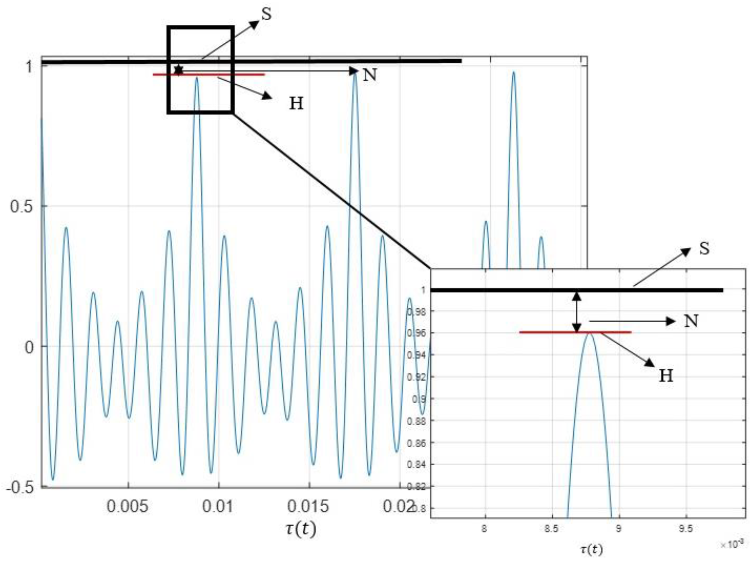
According to the representation of the normalized Autocorrelation represented in Figure 2, the signal S = 1, and the Harmonic component is the Autocorrelation value H = A. NHR is the relationship between the noise (given by the difference between the total signal—S, and the Harmonic component—H) and the Harmonic component. Therefore, Equations (4) and (5) provide the NHR. This relationship is not the one used by Boersma [32], where NHR = 1 − A. Equation (5) is close to 1 − A for A ≈ 1, which happens for most signals corresponding to the normophonic sustained vowels.
For S = 1, and A = H,
2.3.3. Harmonic to Noise Ratio—HNR
The HNR is a parameter in which the relationship between harmonic and noise components provides an indication of the voiced components of the speech signal by quantifying the relationship between the periodic and aperiodic components, expressed in dB [38,39,40]. This measurement relates to the energy conveyed by the voiced signal through the glottal impulses and the energy of the glottal noise fraction after being filtered through the vocal tract. This noise arises from the turbulence generated when the airflow passes through the glottis during phonation, occurring when, for example, the vocal folds close inappropriately [37,38]. A signal’s overall HNR value varies because different vocal tract configurations give different amplitudes for harmonics. Various approaches can be used to determine the HNR automatically. For instance, [41,42] used the cepstrum to measure the harmonic and noise components, while [27,43] used the Autocorrelation in the time domain.
Considering that a signal x(t) has additive harmonic and noise components, in the frequency domain, it can be expressed as in Equation (6).
where X(w) corresponds to the speech signal, H(w) to the harmonic component, and N(w) to the noise component in the frequency domain.
The HNR is a logarithmic measure of the energy ratio associated with the harmonic and noise components. Through Equation (7), it is possible to integrate the spectral power over the audible range of frequencies [44].
The spectral power of the harmonic components, expressed by the nominator in Equation (7), corresponds to the power of the harmonic components determined in the Autocorrelation function (H). The spectral power of the noise, expressed by the denominator in Equation (7), corresponds to the remaining power defined in the Autocorrelation function as N.
The proposed method for the HNR determination is based on the Autocorrelation, as described above, and previously used by Boersma in [27]. This method determines HNR according to Equation (8).
From the normalized Autocorrelation, and considering S = 1, and H = A (Autocorrelation), according to Figure 2,
2.4. Efficient Algorithm for Autocorrelation, HNR, and NHR Determination
The purpose of developing this algorithm is to be implemented in a medical decision support system to detect speech pathologies.
Teixeira and Gonçalves, 2016 [43], implemented an algorithm to determine the jitter, shimmer, and the HNR. However, the authors claim the need to improve the HNR determination. In addition, Fernandes et al., in 2018 [37] had already explored the selection of window shapes and length, but using the ax(τ) and without the division referred to in Equation (3) in the algorithm. They selected longer windows lengths, but the error was higher than with this new algorithm. This algorithm project is an attempt to reduce the computational complexity and improve the quality of Autocorrelation, HNR, and NHR measurement.
As mentioned in the description of the parameters, the determination of the Autocorrelation is the base for the determination of the other parameters. Therefore, the main concern here is the correct determination of the Autocorrelation. The Autocorrelation determination is sensitive to the type of window and its length. Therefore, several combinations were tested.
The method used for the window length selection considers multiples lengths of glottal periods. The glottal period is the inverse of the fundamental frequency fo. The fo is determined using the Autocorrelation method with a frame window length of 100 ms and considering a minimum fo of 50 Hz. The initial fo is determined with a frame window from the middle of the speech record, and then it is updated for each new frame of the analysis.
Then, the normalized Autocorrelation of the Hanning window with a length of 6 glottal cycles is determined.
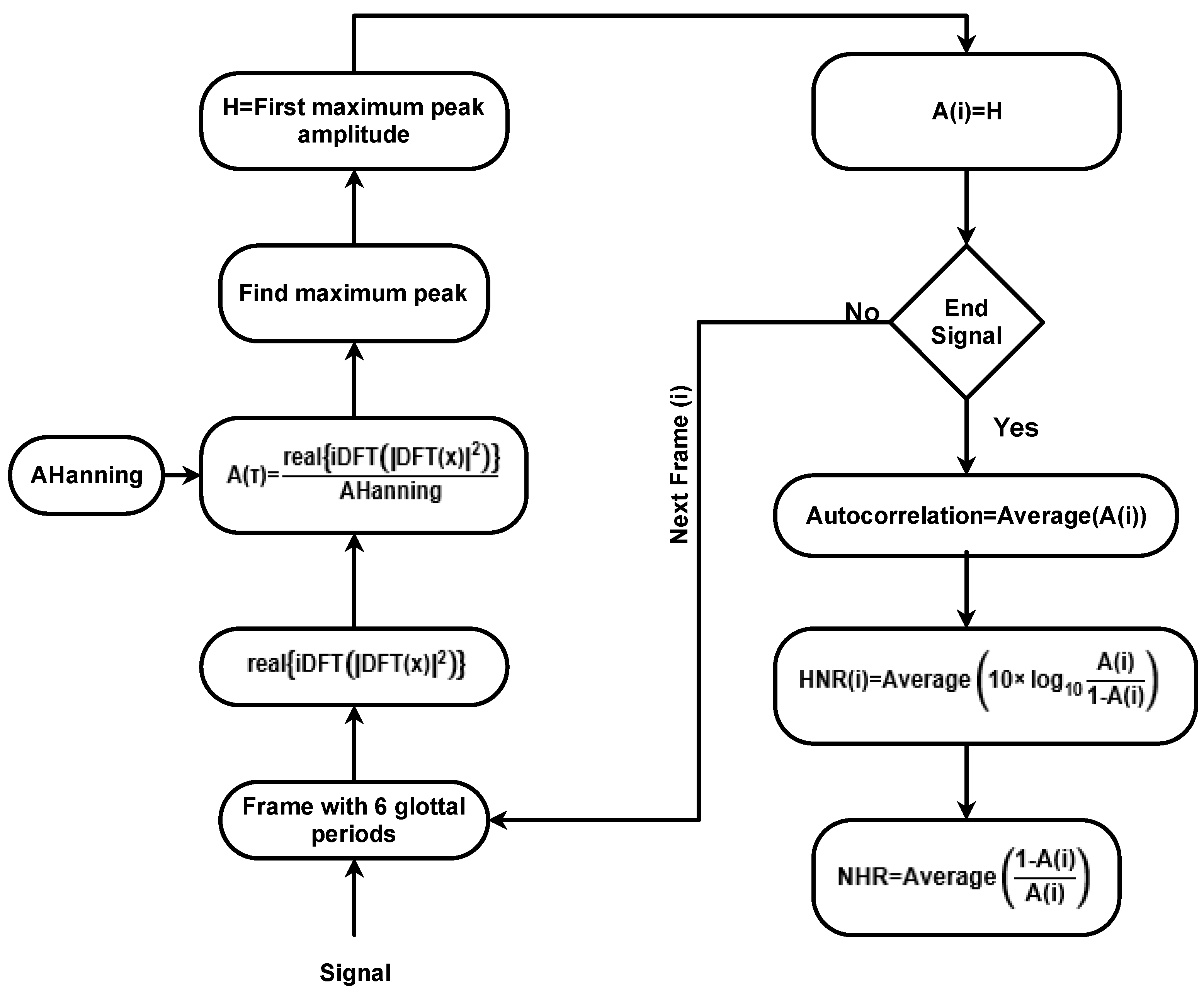
Segmenting the signal into frames, which have a length of 6 glottal cycles, is necessary. Each frame is multiplied by a Hanning window of the same size, and the normalized Autocorrelation of the frame is determined. Then it is divided by the normalized Autocorrelation of the window. At that time, it is necessary to find the first maximum peak in half of the segment between 0.002 and 0.03 s. These values assume that fo is between 33 and 500 Hz. The Autocorrelation is considered to be the magnitude of this peak. Finally, the HNR is calculated for each peak using Equation (9). According to the results in the following section, the next frame is assumed without overlapping. After determining these values for all frames, the Autocorrelation and the HNR are averaged. Through Figure 3, it is possible to observe the flowchart of the developed algorithm.
Some advantages of this algorithm over other time domain algorithms for HNR determination are as follows:
- It allows the determination of Autocorrelation, HNR and NHR at once with the same window and window length. The best window and window length are presented in the following sections.
- Determining the Autocorrelation’s first peak is more straightforward (less complex and more efficient) than other algorithms, such as Boersman’s [27].
- No overlapping is used because the results are the same for sustained vowels.
For a complexity analysis of the proposed algorithm, a time and space analysis is presented [45,46]. In this analysis, n is the length of all audio signals, and m is the length of each segment (the length of the number of glottal cycles). Therefore, m can be considered approximately constant for each audio file. Once there is no overlapping, the loop of Figure 3 will be repeated n/m times. Therefore, the time complexity of the loop is O(n). The main operation in the loop is the peak determination, which is also O(n) for the whole audio.
The main loop of Figure 3 is the normalized Autocorrelation determination implemented by operations in Equation (10), using the Wiener–Khintchine theorem [47,48].
where AHanning denotes the Autocorrelation of the Hanning window vector (determined outside of the loop and stored in a vector), x is the segment signal with six glottal periods length, DFT denotes the Discrete Fourier Transform (DFT), iDFT is the inverse DFT, and real is the real part of the complex signal.
This implementation requires the determination of the DFT. It is efficiently determined by the Cooley–Tukey Fast Fourier Transform (FFT) algorithm. For a given segment, the time complexity of this algorithm to obtain the FFT a is O(m × log(m)), considering an efficient implementation of the FFT transform, such as Cooley–Tukey, is used. For the whole audio, the time complexity is . It is noticeable, however, that m behaves as a constant value. Consequently, the time complexity for the whole audio is O(n). The inverse FFT is determined based on the FFT algorithm and has the same complexity. Regarding memory, the proposed algorithm allocates the audio and support variables, whose size is considered constant, resulting in O(n) space complexity.
2.5. Methodology of the Analysis of Results
A comparative analysis is presented in the Section 3 for the HNR and Autocorrelation values between the values obtained by the algorithm and Praat software to know the best window length and the best window shape to use.
We also present an estimation of how HNR and Autocorrelation vary with the sampling frequency.
The comparison was made using the 9 files with recorded speech for 10 control subjects and 10 patient subjects, in a total of 180 measurements for each analysis. It was decided not to use all the subjects in the database because, in several cases, there is at least one of the 9 sound files with poor acoustic quality. This lousy quality consists of having silent parts, or the voice does not present voicing characteristics, and therefore does not contain harmonic content. The measurement of the parameters in these cases results in meaningless values, which are statistically considered outliers. Thus, it was decided to select 10 control and 10 pathological subjects, in which all recordings are without defects.
Hamming, Hanning, and Blackman windows were tested. For each window shape, 4 window lengths were used, corresponding to 3, 6, 12, and 24 glottal cycles. Using the Autocorrelation method, the glottal cycle is pre-determined in the middle of the speech signal record and adjusted in each cycle. These window lengths were based on the values experimented with in [27], which used the same window lengths. Gonçalves 2015 [43] tested 5, 10, 20, and 50 glottal cycles, and selected the 10 glottal cycles length.
The overlapping of windows was also tested. The Autocorrelation and HNR values were similar to those that did not have a window overlap. Therefore, to reduce the computational weight of the algorithm, it was decided to use the algorithm with zero overlapping over windows. This option is acceptable because the signals used are mainly stationary. For non-stationary signals, the use of overlapping should be considered. In this case (zero overlapping), the number of frame windows is proportional to the signal length. Otherwise, it depends on the degree of overlap.
Concerning the Praat software used as the reference, the default parameters were used [49], namely:
- Time step over windows of 10 ms (overlapping). This value corresponds to the interval between successive frame values.
- Minimum fo = 75 Hz. This value is used to limit the length of admissible fundamental periods and the analysis window length.
- Silence threshold: standard value, 0.1. Frames that do not contain amplitudes above this threshold (relative to the global maximum amplitude) are considered silent.
- Number of cycles per window: standard value, 4.5.
- Window used: Hanning.
Boersma (1993) [27] argues that 4.5 cycles of speech are best for speech HNR values up to 37 dB because it is guaranteed to be detected reliably, and 6 cycles per window raise this figure to more than 60 dB, but the algorithm becomes more sensitive to dynamic changes in the signal.
3. Results
In order to understand how the algorithm behaves, an analysis was performed in which a signal was generated and the HNR and Autocorrelation were measured, using the reference software and the algorithm.
Another analysis was carried out using the USP database, where 10 pathological and 10 normophonic subject’s audio records were selected. For each subject, the vowel /a/ was used. This analysis compares HNR and Autocorrelation values using the algorithm and reference software.
3.1. Windows Type and Length Selection
For the 10 control subjects and the 10 pathological subjects, the Autocorrelation and HNR were extracted using the developed algorithm for nine speech samples (three vowels × three tones) with the three windows (Hamming, Hanning, and Blackman) and, for each window, four lengths (3, 6, 12, and 24 glottal periods). Praat software also determined the Autocorrelation and HNR for the same speech samples. The difference in HNR and Autocorrelation between the algorithm and Praat was determined for each speech sample. Finally, the differences were averaged for all 90 patient samples (average over 90 values) for each window and length.
Table 1 presents the mean of absolute differences and standard deviation for each window/length. The goal is to find the window type and length similar to the Praat reference values.
From Table 1, it can be observed that for the HNR for the patients, the smallest difference (in bold) occurs with a Hanning window with six cycles (0.26 dB). The smallest difference for the control subjects is obtained with the Hanning and Blackman windows with six glottal cycles (0.42 and 0.40 dB). Since only one of the windows can be chosen, the Hanning window is the best one, considering controls and patient subjects.
For the Autocorrelation, the best results are obtained with the three windows types for six glottal cycles (in bold). The smallest difference is 0.001 for the control group and 0.004 for the pathological group.
In conclusion, for the determination of the Autocorrelation using six glottal cycles with one of the Hanning, Hamming, or Blackman windows gave the closest match to the results obtained using the default settings in Praat.
3.1.1. HNR
The average absolute difference can hide some high discrepancies, so it follows an individual comparison over the 180 measurements. For the algorithm, the window chosen was that previously mentioned, Hanning, with a length of six glottal cycles.
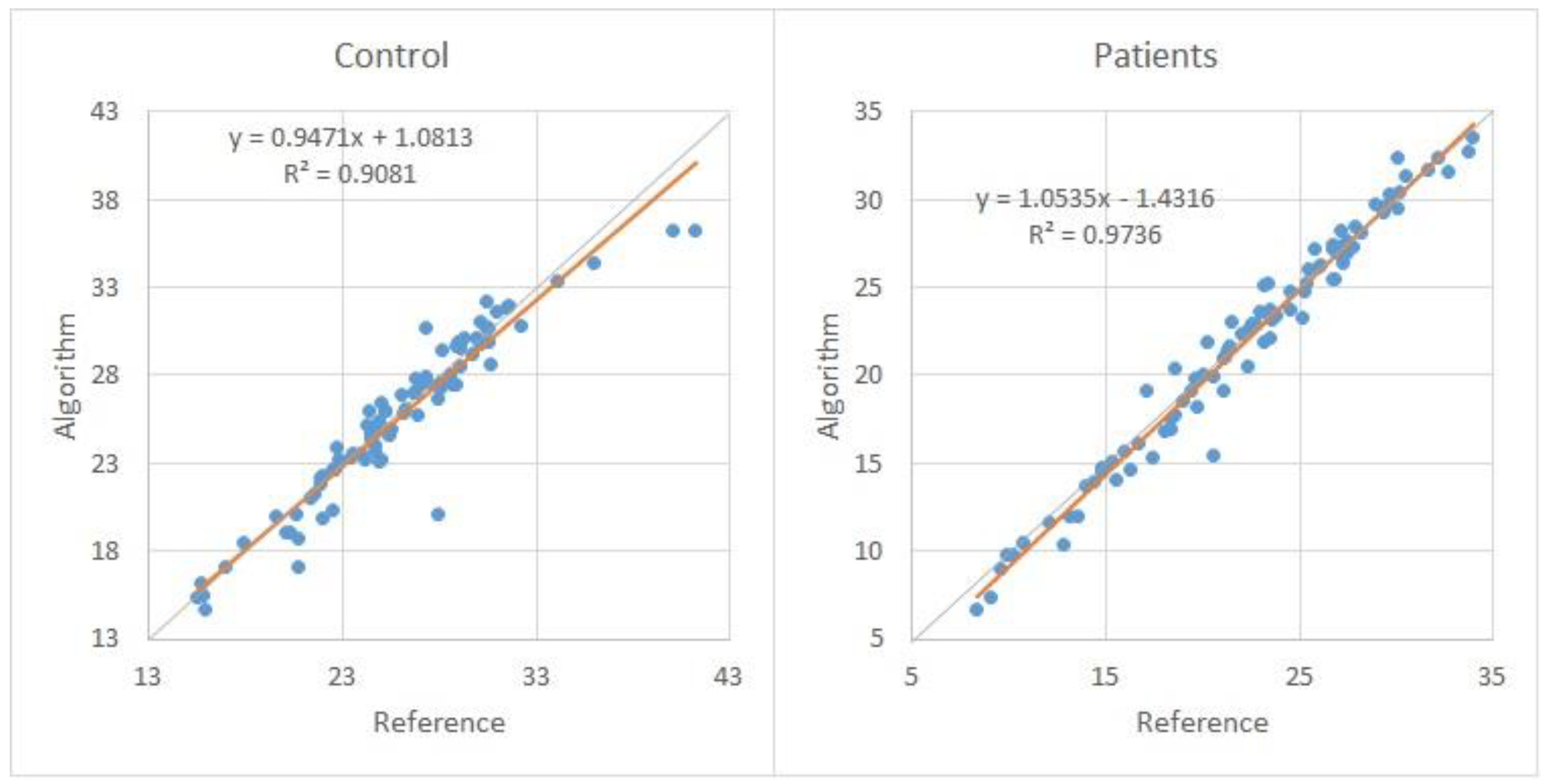
Figure 4 shows the scatter plot of the 90 HNR measurements over 10 control subjects (left-hand side) and 90 measurements for 10 pathological subjects (right-hand side). Each subject has nine HNR measurements for three vowels, and each vowel has three tones. These measurements were determined by the developed algorithm and by the reference software (Praat).
From the previous figure, it is possible to observe that the results of the HNR of the algorithm and reference are very similar since the individual HNR is very close.
3.1.2. Autocorrelation
Similarly, as for HNR, an individual Autocorrelation analysis was made, considering the values for each subject. The Hanning window with six glottal cycles was used.
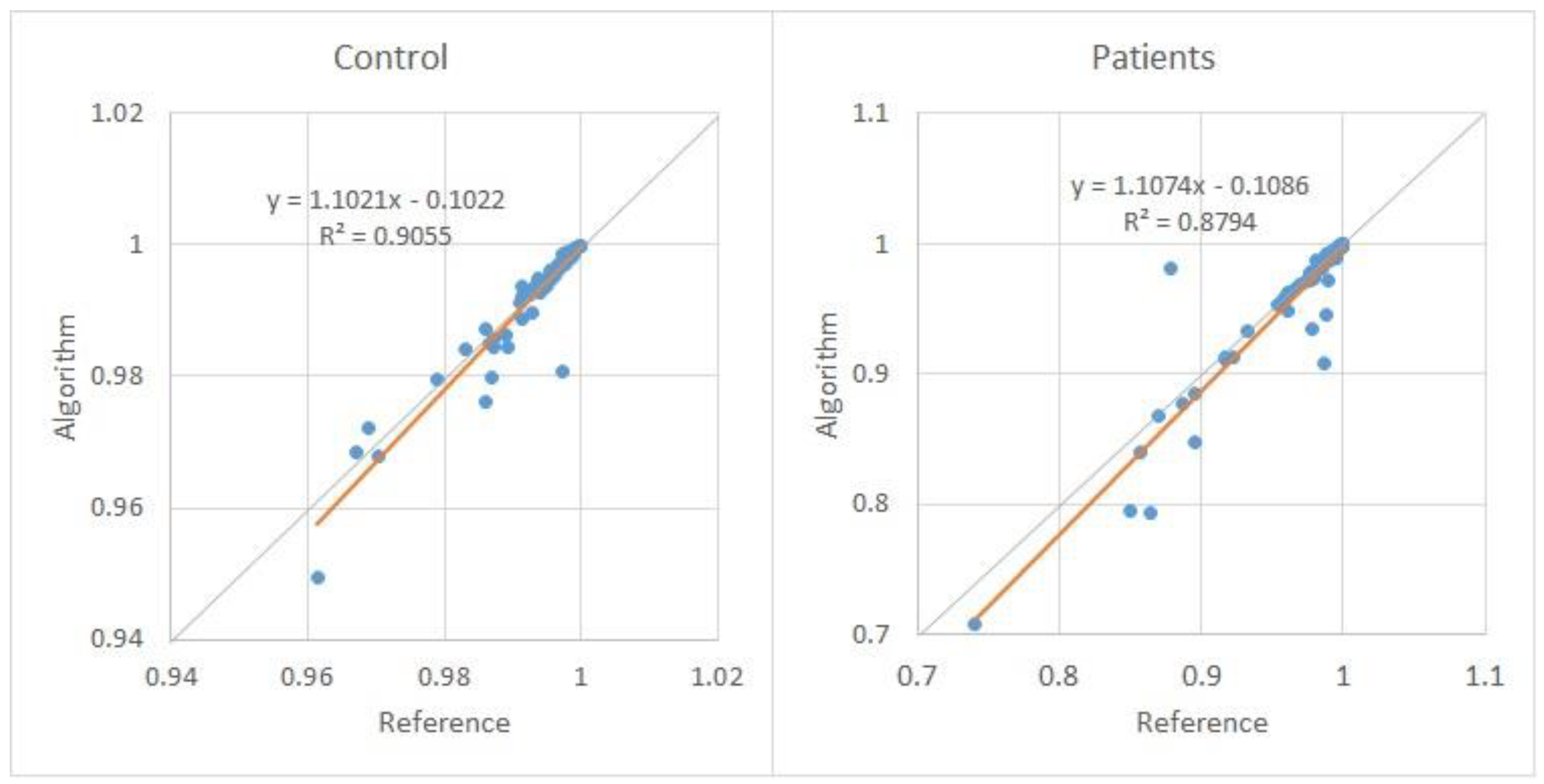
In Figure 5, it is possible to observe the scatter plot of the 90 Autocorrelation measurements over 10 control subjects (left-hand side), and 90 measurements for 10 pathological subjects (right-hand side). Each subject has nine Autocorrelation measurements for three vowels, and each vowel has three tones. These measurements were determined by the developed algorithm and by the reference software (Praat).
Figure 5 shows that the results obtained by the algorithm and the reference for the Autocorrelation are almost identical, with a large part of the values overlaid.
Thus, for the Autocorrelation, the window can be a Hanning, Hamming, or Blackman window with a length of six glottal cycles.
3.1.3. NHR
The NHR parameter is determined as a function of Autocorrelation (1-A)/A. Therefore, the analysis to compare the NHR values of the algorithm with Praat was not performed because it was already completed for the Autocorrelation parameter. However, the subjects’ analysis was performed to understand how the algorithm behaves compared to the reference value.
For the NHR, the Hanning window with six glottal cycles was also used since it is the value used for Autocorrelation.
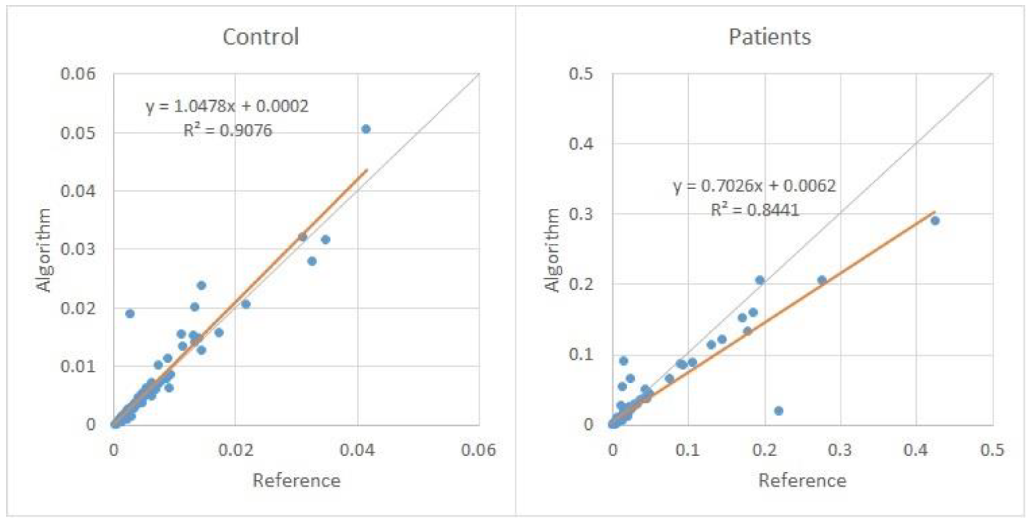
Figure 6 shows the scatter plot of the 90 NHR measurements over 10 control subjects (left-hand side), and 90 measurements for 10 pathological subjects (right-hand side). Each subject has nine NHR measurements for three vowels, and each vowel has three tones. These measurements were determined by the developed algorithm and by the reference software (Praat).
Through Figure 6, it is possible to observe that the results obtained by the algorithm and the reference to the NHR are practically identical.
In conclusion, this algorithm obtains values very close to the reference values and can be used to extract this parameter.
3.2. Sensitivity to the Sampling Frequency Variation
In order to test how the algorithm behaves in the determination of Autocorrelation and HNR with the variation of the sampling frequency, the same sounds were decimated (resampled) from the original 50 kHz to the sampling frequency of 25 kHz and 12.5 kHz.
The decimation process intends to reduce the original sampling frequency. An anti-aliasing digital low-pass filter preceded the decimation process. The Chebyshev Type I of order 8 was used.
For this analysis, the same method was used for the original signal with 50 kHz to determine the best window and glottal period. However, in this case, only the Hanning window with six glottal cycles was used since this window and length obtained the best results for the two parameters previously.
Table 2 presents a similar analysis as previously, now only with the Hanning window and six glottal cycles, but for 25 kHz and 12.5 kHz. The HNR and Autocorrelation values obtained by the algorithm for these sampling frequencies were compared with the reference value for the signal with 50 kHz (original signal). The comparison also consists of determining the average of the individual sample differences (90 samples for each group).
The data in Table 2 show a slight increase in the HNR differences in the value measured by the algorithm compared to the values obtained with the sampling frequency of 50 kHz. This increase is more accentuated for Fs of 12.5 kHz. For the Autocorrelation, the results are similar to those obtained with the sampling frequency of 50 kHz. There is an insignificant variation in the patients and control subjects for 25 kHz and 12.5 kHz.
Then, the mean and standard deviation of all HNR values determined by the algorithm and the reference software for the three values of sampling frequency were compared.
Table 3 shows the average HNR considering all control subjects and patients, for the nine audio samples per subject (180 samples in total), with the Hanning window and six glottal cycles in the algorithm.
Through the analysis of Table 3, it is possible to observe that the HNR for the values of the algorithm varies with the sampling frequency and has a maximum variation of 2.04 dB. The Autocorrelation has a slight variation since the difference along Fs is 0.001 for the algorithm and 0.004 comparing the algorithm with the reference value.
Therefore, it can be concluded that the sampling frequency does not influence the Autocorrelation value in the algorithm.
3.2.1. HNR
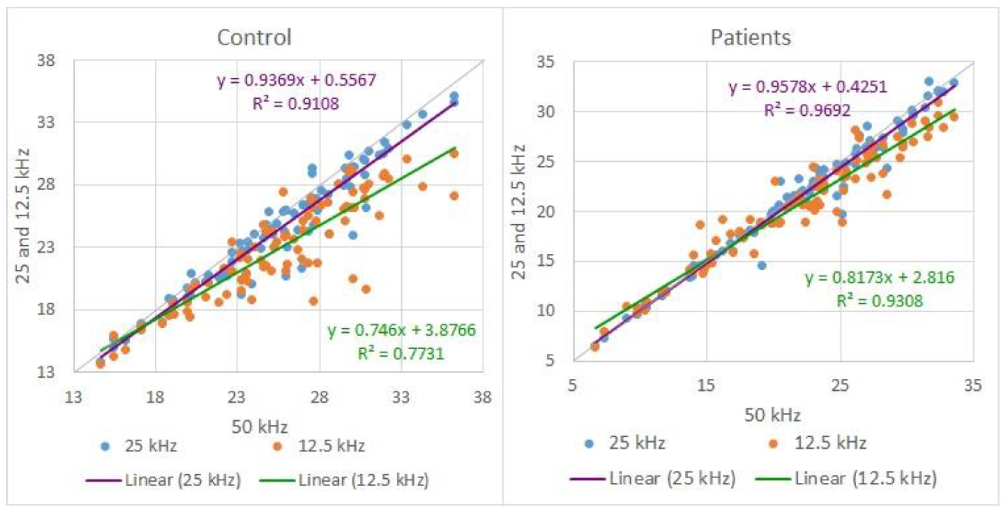
Since the values of the algorithm for the HNR vary somewhat with the sampling frequency, a comparative analysis was made between the three sampling frequencies for the 90 control and patient acoustic records. In Figure 7, it is possible to observe the scatter plot for 25 and 12.5 kHz of the 90 HNR measurements over 10 control subjects (left-hand side), and 90 measurements for 10 pathological subjects (right-hand side). Each subject has nine HNR measurements for three vowels, and each vowel has three tones.
From Figure 7, it is possible to observe some variations in the measurement of HNR. The variations occur mainly in the measurement with Fs of 12.5 kHz in both control and pathological subjects.
Since this variation exists as a function of the sampling frequency, a second analysis was performed to ensure that the algorithm could be used to extract the HNR for the distinction between pathological and normophonic subjects. Therefore, the average of all 20 subjects (90 sounds for control and 90 for patients) as a function of the sampling frequency is presented in Table 4.
Table 4 shows that even though there is a variation of HNR with the sampling frequency, there still is a difference in the average HNR between the pathological and control groups. This critical difference is higher at 50 kHz.
It is concluded that this algorithm can be used cautiously to determine HNR parameters with lower sampling frequency. When the sampling frequency is lowered, the Nyquist frequency of the signal is reduced, losing noise components, which can influence this measure. The minor difference between pathological and control subjects is 2.26 dB, which is indicative of the relevance of the HNR to distinguishing normophonic from pathological speech.
3.2.2. Autocorrelation
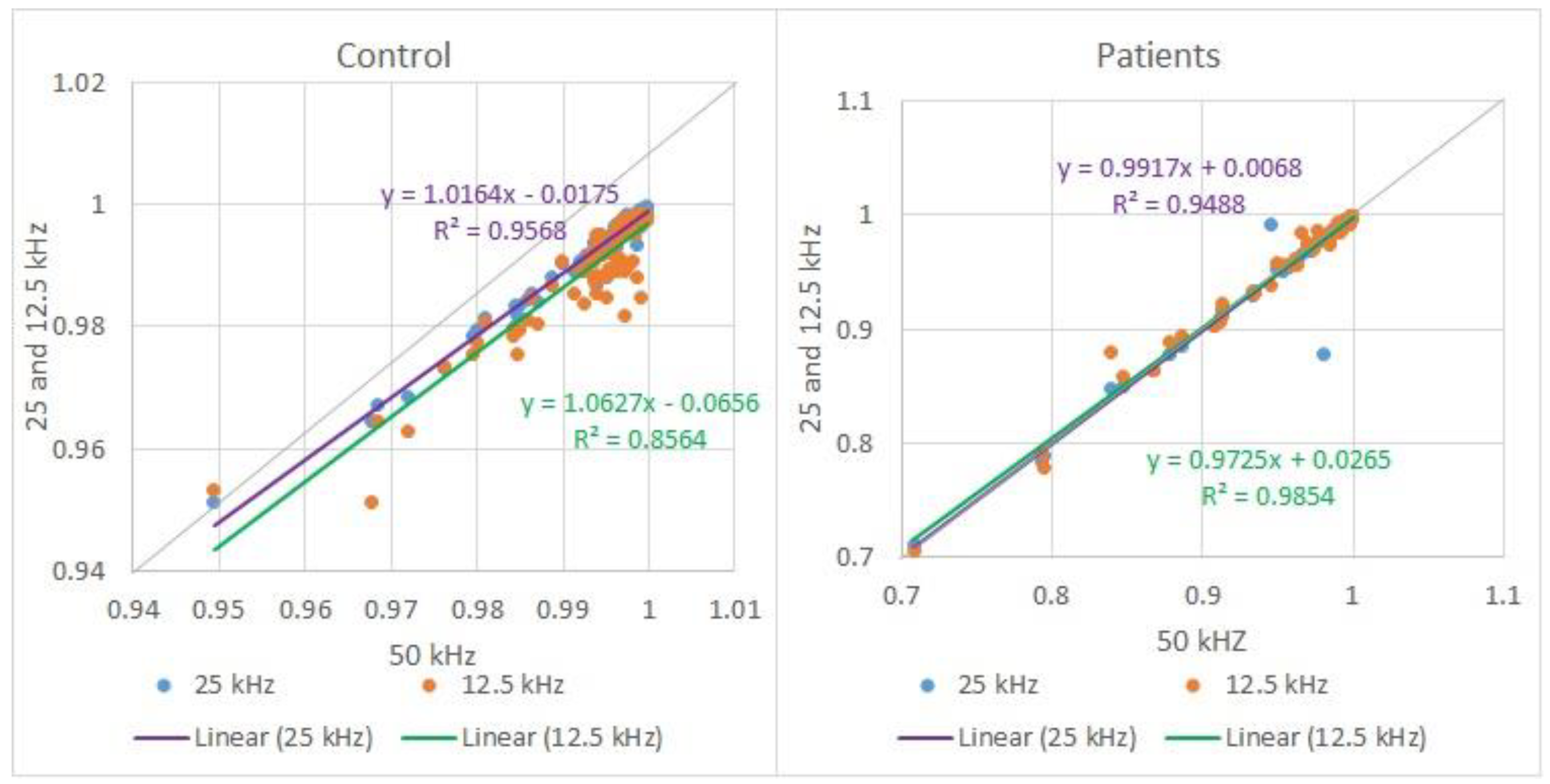
Although the values for the Autocorrelation did not vary with the sampling frequency, a comparative analysis was made between the three sampling frequencies for the 90 control and pathological audios. In Figure 8, it is possible to observe the scatter plot for 25 and 12.5 kHz of the 90 Autocorrelation measurements over 10 control subjects (left-hand side), and 90 measurements for 10 pathological subjects (right-hand side). Each subject has nine Autocorrelation measurements for three vowels, and each vowel has three tones.
From Figure 8, it is possible to observe that the Autocorrelation is just slightly influenced by the frequency variation, as previously confirmed.
3.3. Additional Measures
Through the analyses carried out previously, it was possible to perceive that the values obtained with the algorithm and with the reference software are very similar. However, two more analyses were carried out to guarantee that the values were reliable. Using a generated signal, the first analysis compares algorithm reference software HNR and Autocorrelation measurements. The second analysis compares the algorithm values with the reference software using audio files from the USP database.
3.3.1. Generated Signal
A pure sinusoidal wave was generated with a frequency of 250 Hz, sampling frequency of 44,100 Hz, and an amplitude of 10. White noise with an amplitude of 1 was added.
Table 5 shows that the values obtained by the reference software and by the algorithm are identical.
3.3.2. USP Database Comparison
Additional comparative analysis was made on HNR and Autocorrelation measurements between the algorithm and the reference software. Table 6 presents the comparison. The last line shows the mean absolute difference and standard deviation.
4. Discussion
Autocorrelation, HNR, and NHR were analyzed to understand if this efficient algorithm obtains values close to the reference values for control and pathological voices. The availability of an efficient algorithm allows the depuration of support diagnosis systems into hardware devices with lower computational power.
Concerning the complexity of the proposed algorithm, it has a linear complexity behavior both in time and space. Boerma’s algorithm [27] seems to have the same complexity level, but the proposed algorithm can be faster because of no overlapping requirement. Additionally, and according to the description of the Praat algorithm [27], it considers several peak candidates in the normalized Autocorrelation and takes the candidate in the voiced speech part with the highest value of the local strength, determined according to the rules defined (requiring additional calculus). In opposition, the method used in this algorithm straightly considers the peak as the highest value of the normalized Autocorrelation between 0.002 and 0.030 s (33 < fo < 500 Hz). This difference between the algorithms is acceptable because the Praat algorithm is adequate to be used with voiced and unvoiced parts of speech; meanwhile, the proposed algorithm is supposed to be used only with voiced speech parts of the signal.
Sousa, in 2009 [29], compared the measure of HNR in synthesized and pathologic human voices using time-, spectral-, and cepstral-based methods. The mean absolute errors for synthesized voices were 0.11, 0.52, and 0.61 dB for time- (using Boersma’s algorithm [27]), spectral-, and cepstral-based algorithms using 100 Hz fo voices, respectively. For human pathologic voices, the HNR difference measured by the three methods was up to 1.93 dB for male voices and 3.68 dB for female voices. The author mentions a lower variation in time domain algorithms for different voices. The efficient algorithm presented in this manuscript has an average absolute difference of HNR of 0.26 (σ = 0.29) dB for pathological voices and 0.42 (σ = 0.23) dB for normophonic voices, compared to the same Boersma’s algorithm. The efficient algorithm presents results consistent with the best results in the literature.
The differences in the efficient algorithm are also insignificant compared to the differences presented in [24], where the average HNR Hand marked with 21.31 dB received average HNR from commercial systems with a difference between 3 and 10 dB. Compared to this efficient algorithm, this difference shows a much higher inconsistency between commercial systems software to determine HNR.
This algorithm is being used to develop a diagnostic support device in a hospital environment. In the future, it could also be used on a mobile device or mobile app for tracking purposes. The use of low-power devices in the field presents issues such as the background noise and speaker voice level that may not be well controlled. It is assumed that voice Sound Pressure Level (SPL) would be monitored because the measurement of voice perturbation features, including Autocorrelation, HNR, and NHR, are highly affected by SPL and fo [50].
5. Conclusions
In this work, the SVD database was used, since it presents voice signals of sustained vowels and speech signals of a sentence, which are the required conditions for the type of analysis intended.
An algorithm was developed to determine the HNR, the Autocorrelation, and the NHR. The algorithm uses an integer number of glottal periods to determine the frame to be analyzed, so it was necessary to compare the algorithm values and the reference values. The selection of windows and their length were optimized.
One of the analyses was to search for the best window contour and length so that the value of the parameters was as close as possible to the reference value.
For the HNR parameter, the patient subjects’ samples obtained the lower difference using a Hanning window with six glottal cycles, and for normophonic voices, the Hanning or Blackman window, both with six glottal cycles.
In the comparative analysis between subjects, it is possible to perceive that the values of HNR of the algorithm and reference software are pretty close.
Therefore, considering both groups of subjects, a Hanning window with six glottal cycles was selected.
For the Autocorrelation, the objective is also to know the best window and length to obtain, through the algorithm, the value for this parameter as close as possible to the reference value.
Thus, through the analysis made for the Autocorrelation, the three windows (Hamming, Hanning, and Blackman) with six glottal cycles obtain the lower difference.
However, the Hanning window with six glottal cycles will be considered because, as seen in the flowchart of Figure 3, it allows the processing of Autocorrelation and HNR simultaneously, reducing the computational load.
In the comparative analysis between subjects, it is possible to observe that the results obtained by the algorithm and the reference for Autocorrelation are practically identical for patient and control subjects.
The window and its length were not analyzed extensively for the NHR since it was completed for Autocorrelation, thus justifying the choice of window and length.
However, the comparative analysis of NHR between subjects was performed, and the results obtained by the algorithm and the reference are practically identical for both cases (patients and control).
A further analysis was made to see if the variation of the sampling frequency influences the Autocorrelation and HNR values. The decimation was made for the same speech samples to have signals with a sampling frequency of 12.5 kHz and 25 kHz.
For HNR, the values of the algorithm vary with the sampling frequency and have a maximum variation of 2.04 dB. Further analysis showed that the variations occur mainly in the measurements with a sampling frequency of 12.5 kHz for all vowels and tones.
For the Autocorrelation, the variation of the sampling frequency is insignificant since the Autocorrelation difference is 0.001 and 0.004, comparing the algorithm values with the reference values. Therefore, the sampling frequency does not significantly influence the Autocorrelation value.
In the analysis of the HNR and the Autocorrelation measurements on the generated signal, it was noticed that the algorithm and the reference software measured the same.
A comparative analysis with the USP database was made. The same mean absolute difference level was noticed on Autocorrelation measurements, and a slight increase on HNR mean absolute difference.
As a final consideration, the proposed efficient algorithm allows the determination of the short-term Autocorrelation, HNR, and NHR using a Hanning window with six glottal periods length without overlapping with results very close to the ones presented by Praat software. The algorithm gives similar measurements at 50 kHz sampling frequency and 25 kHz. The average absolute difference is lower than 0.004 for the Autocorrelation and 0.42 dB for HNR. Future research on the issue is to use the algorithm in a smart support system for vocal analysis, which is already under development.
Author Contributions
Conceptualization, J.F.T.F. and J.P.T.; methodology, J.F.T.F. and J.P.T.; validation, J.F.T.F., D.F., A.C.J. and J.P.T.; investigation, J.F.T.F. and J.P.T.; data curation, J.F.T.F.; writing—original, J.F.T.F., A.C.J. and J.P.T.; writing—review and editing, J.P.T., A.C.J. and D.F.; supervision, J.P.T.; funding acquisition, J.P.T. All authors have read and agreed to the published version of the manuscript.
Funding
This research was supported by Foundation for Science and Technology (FCT, Portugal) through national funds FCT/MCTES (PIDDAC) to CeDRI (UIDB/05757/2020 and UIDP/05757/2020), SusTEC (LA/P/0007/2021), and 2021.04729.BD.
Institutional Review Board Statement
The study was conducted following the Declaration of Helsinki.
Informed Consent Statement
Not applicable.
Data Availability Statement
Data are available at http://www.ipb.pt/~joaopt/produtos/CuredDatabase/base_de_dados_curada.xlsx.
Conflicts of Interest
The authors declare no conflict of interest.
References
- Awan, S.N.; Roy, N. Outcomes Measurement in Voice Disorders: Application of an Acoustic Index of Dysphonia Severity. J. Speech, Lang. Hear. Res. 2009, 52, 482–499. [Google Scholar] [CrossRef] [PubMed]
- Narasimhan, S.V.; Rashmi, R. Multiparameter Voice Assessment in Dysphonics: Correlation Between Objective and Perceptual Parameters. J. Voice 2020, 36, 335–343. [Google Scholar] [CrossRef] [PubMed]
- Fant, G.; Ondrackova, J.; Lindqvist-Gauffin, J.; Sonesson, B. “Electrical glottography”, Dept. for Speech, Music and Hearing Quarterly Progress and Status Report. STL-QPSR J. 1996, 7, 15–21. [Google Scholar]
- Titze, I.R. Principles of Voice Production; National Center for Voice and Speech: Salt Lake City, UT, USA, 1994. [Google Scholar]
- Roy, N.; Gerratt, B.R.; Titze, I.R. A comparison of electroglottography and videostroboscopy in the assessment of glottal closure. J. Acoust. Soc. Am. 1999, 106, 3413–3420. [Google Scholar]
- Zur, O.; Sapienza, C.M. Electroglottographic evaluation of voice therapy. J. Voice 1998, 12, 59–68. [Google Scholar]
- Sapienza, C.M.; Tetnowski, J.A.; Hapner, E.R. Electroglottographic measurement of glottal closure duration during vowel production. J. Acoust. Soc. Am. 2000, 108, 2210–2217. [Google Scholar]
- Brinca, L.; Batista, A.P.; Tavares, A.I.; Pinto, P.N.; Araújo, L. The Effect of Anchors and Training on the Reliability of Voice Quality Ratings for Different Types of Speech Stimuli. J. Voice 2015, 29, e7–e776. [Google Scholar] [CrossRef] [PubMed]
- Jesus, L.M.; Belo, I.; Machado, J.; Hall, A. The Advanced Voice Function Assessment Databases (AVFAD): Tools for Voice Clinicians and Speech Research. In Advances in Speech-Language Pathology; IntechOpen: London, UK, 2017. [Google Scholar] [CrossRef]
- Sataloff, R.T.; Kolte, M.; Lele, J. Common Medical Diagnoses and Treatments in Patients with Voice Disorders: An Introduction and Overview. 2017. Available online: https://entokey.com/common-medical-diagnoses-and-treatments-in-patients-with-voice-disorders-an-introduction-and-overview/ (accessed on 18 September 2022).
- Kadiri, S.R.; Alku, P.; Member, S. Analysis and Detection of Pathological Voice Using Glottal Source Features. IEEE J. Sel. Top. Signal Process. 2020, 14, 367. [Google Scholar] [CrossRef]
- Samlan, R.A.; Story, B.H. Relation of Structural and Vibratory Kinematics of the Vocal Folds to Two Acoustic Measures of Breathy Voice Based on Computational Modeling. J. Speech, Lang. Hear. Res. 2011, 54, 1267–1283. [Google Scholar] [CrossRef]
- Forero M, L.A.; Kohler, M.; Vellasco, M.M.B.R.; Cataldo, E. Analysis and Classification of Voice Pathologies Using Glottal Signal Parameters. J. Voice 2016, 30, 549–556. [Google Scholar] [CrossRef]
- Kolhatkar, K.; Kolte, M.; Lele, J. Implementation of pitch detection algorithms for pathological voices. In Proceedings of the 2016 International Conference on Inventive Computation Technologies (ICICT), Coimbatore, India, 26–27 August 2016. [Google Scholar] [CrossRef]
- Fujimura, S.; Kojima, T.; Okanoue, Y.; Kagoshima, H.; Taguchi, A.; Shoji, K.; Inoue, M.; Hori, R. Real-Time Acoustic Voice Analysis Using a Handheld Device Running Android Operating System. J. Voice 2020, 34, 823–829. [Google Scholar] [CrossRef]
- Gorris, C.; Maccarini, A.R.; Vanoni, F.; Poggioli, M.; Vaschetto, R.; Garzaro, M.; Valletti, P.A. Acoustic Analysis of Normal Voice Patterns in Italian Adults by Using Praat. J. Voice 2020, 34, e9–e961. [Google Scholar] [CrossRef] [PubMed]
- Ankışhan, H.; İnam, S.Ç. Voice pathology detection by using the deep network architecture. Appl. Soft Comput. 2021, 106, 107310. [Google Scholar] [CrossRef]
- Cordeiro, H.T.; Ribeiro, C.M. Spectral envelope first peak and periodic component in pathological voices: A spectral analysis. Procedia Comput. Sci. 2018, 138, 64–71. [Google Scholar] [CrossRef]
- Karlsen, T.; Sandvik, L.; Heimdal, J.H.; Aarstad, H.J. Acoustic Voice Analysis and Maximum Phonation Time in Relation to Voice Handicap Index Score and Larynx Disease. J. Voice 2020, 34, e27–e161. [Google Scholar] [CrossRef] [PubMed]
- Guedes, V.; Teixeira, F.; Oliveira, A.; Fernandes, J.; Silva, L.; Junior, A.; Teixeira, J.P. Transfer Learning with AudioSet to Voice Pathologies Identification in Continuous Speech. Procedia Comput. Sci. 2019, 164, 662–669. [Google Scholar] [CrossRef]
- De Oliveira, A.A.; Dajer, M.E.; Teixeira, J.P. Clustering pathologic voice with Kohonen SOM and hierarchical clustering. In Proceedings of the BIOSIGNALS 2021—14th International Conference on Bio-Inspired Systems and Signal Processing, Online Streaming, 11–13 February 2021; pp. 158–163. [Google Scholar]
- Guedes, V.; Junior, A.; Fernandes, J.; Teixeira, F.; Teixeira, J.P. Long Short Term Memory on Chronic Laryngitis Classification. Procedia Comput. Sci. 2018, 138, 250–257. [Google Scholar] [CrossRef]
- Teixeira, F.; Fernandes, J.; Guedes, V.; Junior, A.; Teixeira, J.P. Classification of Control/Pathologic Subjects with Support Vector Machines. Procedia Comput. Sci. 2018, 138, 272–279. [Google Scholar] [CrossRef]
- Bielamowicz, S.; Kreiman, J.; Gerratt, B.R.; Dauer, M.S.; Berke, G.S. Comparison of voice analysis systems for perturbation measurement. J Speech Hear Res. 1996, 39, 126–134. [Google Scholar] [CrossRef]
- Teixeira, J.P.; Fernandes, P.O. Acoustic Analysis of Vocal Dysphonia. Procedia Comput. Sci. 2015, 64, 466–473. [Google Scholar] [CrossRef]
- Cantarella, G.; Baracca, G.; Pignataro, L.; Forti, S. Assessment of dysphonia due to benign vocal fold lesions by acoustic and aerodynamic indices: A multivariate analysis. Logop. Phoniatr. Vocology 2011, 36, 21–27. [Google Scholar] [CrossRef] [PubMed]
- Boersma, P. Acurate Short-Term Analysis of the Fundamental Frequency and the Harmonics-to-Noise Ratio of a Sampled Sound. 1993. Available online: http://www.fon.hum.uva.nl/paul/papers/Proceedings_1993.pdf (accessed on 18 September 2021).
- Yegnanarayana, A.L.B.; Darsinos, V. Decomposition of speech signals into deterministic and stochastic components; Decomposition of speech signals into deterministic and stochastic components. In Proceedings of the 1995 International Conference on Acoustics, Speech, and Signal Processing, Detroit, MI, USA, 9–12 May 1995; Volume 1, pp. 760–763. [Google Scholar] [CrossRef]
- De Sousa, R.J.T. A new accurate method of harmonic-to-noise ratio extraction. In Proceedings of the International Conference on Bio-Inspired Systems and Signal Processing—BIOSIGNALS, Porto, Portugal, 14–17 January 2009; pp. 351–356. [Google Scholar] [CrossRef]
- Deliyski, D.D. Acoustic model and evaluation of pathological voice production. In Proceedings of the Third European Conference on Speech Communication and Technology, EUROSPEECH 1993, Berlin, Germany, 22–25 September 1993. [Google Scholar]
- Qi, Y.; Hillman, R.E. Temporal and spectral estimations of harmonics-to-noise ratio in human voice signals. J. Acoust. Soc. Am. 1997, 102, 537–543. [Google Scholar] [CrossRef]
- Boersma, P. Stemmen meten met Praat. Stem Spraak Taalpathol. 2004, 12, 237–251. [Google Scholar]
- Fernandes, J.F.T.; Freitas, D.; Teixeira, J.P. Voice Pathologies: The Most Commom Features and Classification Tools. In Proceedings of the 2021 16th Iberian Conference on Information Systems and Technologies (CISTI), Chaves, Portugal, 23–26 June 2021. [Google Scholar] [CrossRef]
- Chronic Laryngitis. Medical Dictionary. 2009. Available online: https://medical-dictionary.thefreedictionary.com/Chronic+laryngitis (accessed on 10 November 2021).
- Dysphonia. Miller-Keane Encyclopedia and Dictionary of Medicine, Nursing, and Allied Health, Seventh Edition. 2003. Available online: https://medical-dictionary.thefreedictionary.com/dysphonia (accessed on 10 November 2021).
- Pützer, M.; Saarbruecken, W.J.B. Voice Database. Institute of Phonetics at the University of Saarland. 2007. Available online: http://www.stimmdatenbank.coli.uni-saarland.de (accessed on 5 November 2021).
- Fernandes, J.; Teixeira, F.; Guedes, V.; Junior, A.; Teixeira, J.P. Harmonic to Noise Ratio Measurement—Selection of Window and Length. Procedia Comput. Sci. 2018, 138, 280–285. [Google Scholar] [CrossRef]
- Jalali-najafabadi, F.; Gadepalli, C.; Jarchi, D.; Cheetham, B.M.G. Acoustic analysis and digital signal processing for the assessment of voice quality. Biomed. Signal Process. Control 2021, 70, 103018. [Google Scholar] [CrossRef]
- Gómez-García, J.A.; Moro-Velázquez, L.; Arias-Londoño, J.D.; Godino-Llorente, J.I. On the design of automatic voice condition analysis systems. Part III: Review of acoustic modelling strategies. Biomed. Signal Process. Control 2021, 66, 102049. [Google Scholar] [CrossRef]
- Vashkevich, M.; Rushkevich, Y. Classification of ALS patients based on acoustic analysis of sustained vowel phonations. Biomed. Signal Process. Control 2021, 65, 102350. [Google Scholar] [CrossRef]
- Murphy, P.J. A cepstrum-based harmonics-to-noise ratio in voice signals. J. Speech Hear. Res. 1993, 36, 254–266. [Google Scholar]
- Murphy, P.J.; Akande, O.O. Cepstrum-Based Estimation of the Harmonics-to-Noise Ratio for Synthesized and Human Voice Signals. In Proceedings of the International Conference on Nonlinear Analyses and Algorithms for Speech Processing, Barcelona, Spain, 19–22 April 2005; p. 3817. [Google Scholar]
- Teixeira, J.P.; Gonçalves, A. Algorithm for Jitter and Shimmer Measurement in Pathologic Voices. Procedia Comput. Sci. 2016, 100, 271–279. [Google Scholar] [CrossRef]
- Shama, K.; Krishna, A.; Cholayya, N.U. Study of harmonics-to-noise ratio and critical-band energy spectrum of speech as acoustic indicators of laryngeal and voice pathology. In Proceedings of the EURASIP Journal on Advances in Signal Processing; Springer Nature: Berlin/Heidelberg, Germany, 2007. [Google Scholar] [CrossRef]
- Wilf, H.S. Algorithms and Complexity, 2nd ed.; CRC Press: Boca Raton, FL, USA, 2002. [Google Scholar]
- Cormen, T.H.; Leiserson, C.E.; Rivest, R.L.; Stein, C. Introduction to Algorithms, 2nd ed.; MIT Press: Cambridge, MA, USA, 2001. [Google Scholar]
- Champeney, D.C. Power Spectra and Wiener’s Theorems. A Handbook of Fourier Theorems; Cambridge University Press: Cambridge, UK, 1987. [Google Scholar]
- Khintchine, A. Korrelationstheorie der stationären stochastischen Prozesse. Math. Ann. 1934, 109, 604–615. [Google Scholar] [CrossRef]
- Boersma, P.; Weenink, D. Praat: Doing Phonetics by Computer. Phonetic Sciences, University of Amsterdam. Available online: https://www.fon.hum.uva.nl/praat/ (accessed on 24 November 2021).
- Cai, H.; Ternström, S. Mapping Phonation Types by Clustering of Multiple Metrics. Appl. Sci. 2022, 12, 12092. [Google Scholar] [CrossRef]
Figure 1.
HNR along tones (h—high, l—low, n—neutral) for vowel /a/ (left-hand side), and along vowels (/a/, /i/, /u/) for neutral tone (right-hand side) for dysphonic and control voices. Groups are FD—Functional Dysphonia, HD—Hyperfunctional Dysphonia, PD—Psychogenic Dysphonia, D—Dysphonia and CG—Control Group. Bars represent the mean value ± standard deviation (95% confidence interval). (Adapted and with the courtesy of [25]).

Figure 2.
Determination of NHR from the normalized Autocorrelation.

Figure 3.
Flowchart of the algorithm to determine Autocorrelation, HNR, and NHR.

Figure 4.
Comparison of HNR values for the 90 control measurements (left-hand side) and 90 patient measurements (right-hand side).
Figure 4.
Comparison of HNR values for the 90 control measurements (left-hand side) and 90 patient measurements (right-hand side).

Figure 5.
Comparison of Autocorrelation values for the 90 control measurements (left-hand side) and 90 patient measurements (right-hand side).
Figure 5.
Comparison of Autocorrelation values for the 90 control measurements (left-hand side) and 90 patient measurements (right-hand side).

Figure 6.
Comparison of the NHR values for the 90 control measurements (left-hand side) and 90 patient measurements (right-hand side).
Figure 6.
Comparison of the NHR values for the 90 control measurements (left-hand side) and 90 patient measurements (right-hand side).

Figure 7.
Comparative analysis of the HNR with 25 and 12.5 kHz over 50 kHz sampling frequency.

Figure 8.
Comparative analysis of the Autocorrelation with 25 and 12.5 kHz over 50 kHz sampling frequency.
Figure 8.
Comparative analysis of the Autocorrelation with 25 and 12.5 kHz over 50 kHz sampling frequency.


Table 1.
Comparison of results from Praat and the proposed algorithm: HNR and Autocorrelation average differences and standard deviation for each window and length.
Table 1.
Comparison of results from Praat and the proposed algorithm: HNR and Autocorrelation average differences and standard deviation for each window and length.
| Window | Window Length (No. of Glottal Cycles) | Average of Absolute Differences | |||
|---|---|---|---|---|---|
| HNR (dB) | Autocorrelation | ||||
| Patients | Control | Patients | Control | ||
| Hamming | 3 | 2.47 (σ = 1.43) | 3.60 (σ = 2.08) | 0.005 (σ = 0.003) | 0.001 (σ = 0.001) |
| 6 | 0.42 (σ = 0.29) | 0.50 (σ = 0.31) | 0.004(σ = 0.005) | 0.001(σ = 0.001) | |
| 12 | 1.69 (σ = 0.54) | 2.23 (σ = 0.60) | 0.007 (σ = 0.006) | 0.004 (σ = 0.003) | |
| 24 | 3.10 (σ = 0.76) | 3.88 (σ = 0.97) | 0.018 (σ = 0.015) | 0.009 (σ = 0.007) | |
| Hanning | 3 | 3.33 (σ = 1.81) | 4.95 (σ = 2.61) | 0.006 (σ = 0.004) | 0.002 (σ = 0.001) |
| 6 | 0.26 (σ = 0.29) | 0.42 (σ = 0.23) | 0.004(σ = 0.005) | 0.001(σ = 0.001) | |
| 12 | 1.59 (σ = 0.50) | 2.07 (σ = 0.53) | 0.007 (σ = 0.006) | 0.003 (σ = 0.002) | |
| 24 | 2.94 (σ = 0.74) | 3.68 (σ = 0.94) | 0.017 (σ = 0.0014) | 0.009 (σ = 0.007) | |
| Blackman | 3 | 8.61 (σ = 1.71) | 11.56 (σ = 2.52) | 0.013 (σ = 0.006) | 0.009 (σ = 0.006) |
| 6 | 0.37 (σ = 0.20) | 0.40 (σ = 0.23) | 0.004(σ = 0.004) | 0.001(σ = 0.000) | |
| 12 | 1.21 (σ = 0.52) | 1.66 (σ = 0.43) | 0.006 (σ = 0.005) | 0.002 (σ = 0.002) | |
| 24 | 2.56 (σ = 0.71) | 3.21 (σ = 0.88) | 0.015 (σ = 0.013) | 0.007 (σ = 0.005) | |
Table 2.
HNR and Autocorrelation average differences as a function of sampling frequency.
| Sampling Frequency (kHz) | Average Difference | |||
|---|---|---|---|---|
| HNR (dB) | Autocorrelation | |||
| Patients | Control | Patients | Control | |
| 25 | 0.58 (σ = 0.38) | 1.16 (σ = 0.33) | 0.006 (σ = 0.005) | 0.001 (σ = 0.001) |
| 12.5 | 2.03 (σ = 0.32) | 3.45 (σ = 0.63) | 0.006 (σ = 0.006) | 0.004 (σ = 0.002) |
Table 3.
HNR and Autocorrelation as a function of the sampling frequency.
| Sampling Frequency (kHz) | HNR (dB) | Autocorrelation | ||
|---|---|---|---|---|
| Algorithm | Reference | Algorithm | Reference | |
| 50 | 23.89 (σ = 2.56) | 24.02 (σ = 2.32) | 0.981 (σ = 0.009) | 0.984 (σ = 0.007) |
| 25 | 22.98 (σ = 2.59) | 23.85 (σ = 2.49) | 0.980 (σ = 0.010) | 0.984 (σ = 0.007) |
| 12.5 | 21.85 (σ = 2.55) | 24.59 (σ = 2.33) | 0.980 (σ = 0.010) | 0.984 (σ = 0.007) |
Table 4.
HNR as a function of the Sampling Frequency for the control and patient groups.
| Sampling Frequency (kHz) | Patients (dB) | Control (dB) |
|---|---|---|
| 50 | 21.91 (σ = 2.49) | 25.60 (σ = 2.63) |
| 25 | 21.41 (σ = 2.58) | 24.55 (σ = 2.60) |
| 12.5 | 20.72 (σ = 2.49) | 22.98 (σ = 2.61) |
Table 5.
Autocorrelation and HNR values on a generated signal.
| Reference | Algorithm | |
|---|---|---|
| HNR | 21.79 | 21.78 |
| Autocorrelation | 0.993 | 0.993 |
Table 6.
Comparison of the values obtained by the algorithm with the reference software, for the parameters HNR and Autocorrelation, for the USP database.
Table 6.
Comparison of the values obtained by the algorithm with the reference software, for the parameters HNR and Autocorrelation, for the USP database.
| Samples | HNR | Autocorrelation | ||||||
|---|---|---|---|---|---|---|---|---|
| Patients | Control | Patients | Control | |||||
| Ref. | Alg. | Ref. | Alg. | Ref. | Alg. | Ref. | Alg. | |
| 1 | 32.86 | 30.75 | 15.03 | 13.64 | 0.998 | 0.998 | 0.942 | 0.935 |
| 2 | 18.95 | 17.24 | 19.76 | 18.88 | 0.982 | 0.976 | 0.987 | 0.985 |
| 3 | 19.14 | 18.40 | 20.04 | 19.10 | 0.985 | 0.983 | 0.989 | 0.986 |
| 4 | 19.52 | 19.05 | 22.70 | 20.52 | 0.984 | 0.983 | 0.991 | 0.989 |
| 5 | 24.50 | 23.06 | 25.21 | 22.24 | 0.994 | 0.993 | 0.995 | 0.992 |
| 6 | 24.56 | 23.21 | 22.25 | 21.29 | 0.995 | 0.993 | 0.990 | 0.989 |
| 7 | 18.34 | 17.17 | 18.44 | 16.23 | 0.983 | 0.979 | 0.977 | 0.972 |
| 8 | 19.16 | 18.61 | 21.15 | 19.58 | 0.986 | 0.984 | 0.989 | 0.987 |
| 9 | 14.78 | 14.68 | 23.03 | 20.04 | 0.955 | 0.953 | 0.992 | 0.987 |
| 10 | 19.48 | 18.86 | 23.04 | 21.13 | 0.987 | 0.985 | 0.994 | 0.990 |
| Mean Abs. Difference | 1.03 (σ = 0.53) | 1.80 (σ = 0.66) | 0.002 (σ = 0.001) | 0.003 (σ = 0.002) | ||||
Disclaimer/Publisher’s Note: The statements, opinions and data contained in all publications are solely those of the individual author(s) and contributor(s) and not of MDPI and/or the editor(s). MDPI and/or the editor(s) disclaim responsibility for any injury to people or property resulting from any ideas, methods, instructions or products referred to in the content. |
© 2023 by the authors. Licensee MDPI, Basel, Switzerland. This article is an open access article distributed under the terms and conditions of the Creative Commons Attribution (CC BY) license (https://creativecommons.org/licenses/by/4.0/).
Share and Cite
MDPI and ACS Style
Fernandes, J.F.T.; Freitas, D.; Junior, A.C.; Teixeira, J.P. Determination of Harmonic Parameters in Pathological Voices—Efficient Algorithm. Appl. Sci. 2023, 13, 2333. https://doi.org/10.3390/app13042333
AMA Style
Fernandes JFT, Freitas D, Junior AC, Teixeira JP. Determination of Harmonic Parameters in Pathological Voices—Efficient Algorithm. Applied Sciences. 2023; 13(4):2333. https://doi.org/10.3390/app13042333
Chicago/Turabian StyleFernandes, Joana Filipa Teixeira, Diamantino Freitas, Arnaldo Candido Junior, and João Paulo Teixeira. 2023. "Determination of Harmonic Parameters in Pathological Voices—Efficient Algorithm" Applied Sciences 13, no. 4: 2333. https://doi.org/10.3390/app13042333
Note that from the first issue of 2016, this journal uses article numbers instead of page numbers. See further details here.