
Characterization of Nonlinear Responses of Non-Premixed Flames to Low-Frequency Acoustic Excitations


School of Mechanical and Engineering, Tongji University, Shanghai 201804, China
*
Author to whom correspondence should be addressed.
Appl. Sci. 2023, 13(10), 6237; https://doi.org/10.3390/app13106237
Submission received: 24 April 2023
/
Revised: 12 May 2023
/
Accepted: 17 May 2023
/
Published: 19 May 2023
(This article belongs to the Special Issue Feature Papers in Section 'Applied Thermal Engineering')
Abstract
:Featured Application
Stable design of Combustor in industrial boiler and burner.
Abstract
The response of flames’ heat release to acoustic excitation is a critical factor for understanding combustion instability. In the present work, the nonlinear heat release response of a methane–air non-premixed flame to low-frequency acoustic excitations is experimentally investigated. The flame describing function (FDF) was measured based on the overall CH* chemiluminescence intensity and the velocity fluctuations obtained by the two-microphone method. The CH* chemiluminescence and schlieren images were analyzed for revealing the mechanism of nonlinear response. The excitation frequency ranges from 10 Hz to 120 Hz. The forced relative velocity fluctuation amplitude ranges from 0.10 to 0.50. The corresponding flame Strouhal number (Stf) ranges from 0.43 to 4.67. The study has shown that the flame length responds more sensitively to changes in excitation amplitude when subjected to relatively high-frequency excitations. The normalized flame length (Lf/D) decreases from 3.79 to 2.37 with the increase in excitation amplitude at an excitation frequency of 100 Hz. The number of oscillation zones along the flame increases with increasing excitation frequency, which is consistent with the increase in the Stf. The low-pass filtering characteristic of FDF is caused by the dispersion of multiple oscillation zones, as well as the cancellation effect of the adjacent oscillation zones under relatively high-frequency excitation. The main mechanism for the local gain peak and valley is the cancellation effect of positive and negative oscillation zones with various Stf. When two adjacent oscillation regions have similar amplitudes, the overall phase-lag becomes more sensitive to changes in excitation frequency and amplitude. This sensitivity leads to nonlinear anomalous changes in the phase-lag near the frequency corresponding to the gain valley. The calculated disturbance convection time is consistent with the measured time delay in the short flame scenario. Further research is required to determine whether the identified agreement is a result of the consistent occurrence of the oscillation zone in close proximity to the flame’s center of mass, in conjunction with a precise determination of the average convective velocity.
1. Introduction
Combustion instability has been an issue in combustion equipment with low NOx emissions. It is manifested as large amplitude fluctuations of pressure and heat release in the combustion chamber, which may lead to structural damage. This instability is attributed to the interaction of the unsteady heat release and the cavity acoustic modes of the combustion chamber [1]. Therefore, the response characteristic of heat release rate (HRR) to the flow perturbations is a key factor in better understanding combustion instability [2,3,4]. Previous studies have established related models to describe the response of heat release to flow disturbance. Among them, the n-τ model and the flame transfer function (FTF) were based on the linearization assumption [5,6]. The frequency and the corresponding growth rate of the thermoacoustic oscillations can be predicted through the combination of the linear flame response models and the thermoacoustic coupling model [7]. However, the linear FTF cannot interpret the nonlinear thermoacoustic features, such as the mode switching, nonlinear trigger, and frequency shifting [8], nor can it obtain the oscillation amplitude in limit cycle mode. Therefore, in order to determine the nonlinear response of the flame, the flame describing function (FDF) was proposed [9]. The FDF considers the effects of the forcing amplitude in addition to the frequency. Noiray et al. [10] used the FDF of a premixed flame to interpret the mode-switching phenomenon and predict the limit cycle amplitudes of oscillation. The theoretical results were in excellent agreement with the measurements. FTF and FDF can be obtained through CFD numerical simulation and theoretical analysis and experiments [5,11,12]. With the experiment, the HRR response can be measured using optical equipment, such as PMT, OH-PLIF, or ICCD camera integrated with CH* or OH* chemiluminescence filters [13,14].
Much work has been reported related to the responses of the premixed flame with different configurations, such as laminar conical flames [15,16], multiple conical flames [17], swirled flames [18,19,20], bluff body stabilization flames [21], and practical gas turbine burners [22,23,24]. Compared to the premixed flame, there are relatively few studies on the response characteristics of non-premixed combustion. Existing works mainly focused on the laminar jet diffusion flame. In order to understand the foundational mechanism, a lot of the literature has worked on the forced response of the Burk–Schumann diffusion flame with theoretical analysis. Tyagi et al. [25] theoretically studied the heat release of the Burke–Schumann flame to the longitudinal velocity fluctuations with the assumption of the uniform flow field. It was found that the Da number plays an important role in determining the amplitude and phase of the heat release fluctuations with respect to the velocity fluctuations. Based on the same flame and assumptions, Chandrasekhar and Chakravarthy [26] investigated the response of the flame to transverse velocity oscillations. The gain of heat release response was nearly independent of the amplitude at low frequencies. However, the gain decreased with the increase in the excitation amplitude. Nicholas et al. [27,28] compared the dynamics of the forced response of laminar non-premixed and premixed flames to the velocity fluctuations. Mass burning rate oscillations dominate the response of non-premixed jet flame; however, the perturbations of the flame speed and the burning area induced by the velocity fluctuations caused the oscillations of the HRR for the premixed flame [29]. Corresponding to the different response mechanisms, the gain and phase-lag of the FTF of the jet diffusion flame and premixed flame were also much different, especially under low flame Strouhal number (Stf). Yao and Zhu [30] discussed the distributed FTF for the Burke–Schumann diffusion flame with Green’s Function method. A dual-peak amplitude of the gain was observed in the fuel-rich zone and the fuel-lean zone, respectively. The effects of the Strouhal number, the Peclet number, and convective velocity on hot spot propagation were also discussed, which were related to the entropy wave.
Some experimental work was also conducted to obtain the HRR response of the jet diffusion flame. Jiang et al. [31] studied the forced reacting plumes of a jet non-premixed flame and discussed the interaction of the buoyancy-driven instability and the convective instability. The flame pinch-off was observed with strong low-frequency perturbations and the flame exhibited a low-pass filter characteristic. The dynamics of the jet diffusion flame in a standing wave were studied [32,33,34,35,36]. The low-pass characteristic of the response of the jet diffusion flame was also observed in this geometry. The effects of the excitation frequency and amplitude, the position of the fuel nozzle, and the fuel type on the flame dynamics were discussed in these papers. Kim et al. [37] measured the FDF of a coaxial jet diffusion flame with an excitation frequency ranging from 80 Hz to 200 Hz. The gain of the FDF was independent of the forced amplitude. However, the phase-lag decreased with increasing forced amplitude.
In past research, the non-premixed flame was usually treated as an active control method of combustion instability in premixed flame. However, in recent studies, the self-excited combustion instability of non-premixed flame has also been observed and discussed [38,39]. For the industrial burner, the air and fuel were usually organized in cross-flow jets to enhance the mixing process. In order to anchor the flame, the bluff body was used as the flame stabilization structure. The stabilization mechanism of such bluff body non-premixed flames has been studied [40]. Hardalupas and Selbach [41] investigated the effects of the excitation frequency and the amplitude on the flame lift-off height and the reattachment, as well as the combustion efficiency and emissions of a radial injector non-premixed flame. However, the characteristics of the heat release response to acoustic excitation have not been clearly studied.
Another factor affecting combustion stability is the acoustic characteristics of the combustion chamber cavity, which is mainly determined by its geometric dimensions and the flow field parameters. The natural oscillation mode is presented as a low frequency in practical industrial combustion equipment determined by the geometry parameters of the large cavity [42,43]. Therefore, the response to low-frequency excitation is significant.
In summary, many attempts have been made to understand the response mechanism of the non-premixed flame with different geometries. However, much less data are available for systematic studies of the FTF and FDF of non-premixed flames under acoustic perturbations, especially in experiments. The effects of the excitation frequency and amplitude on the phase-lag and gain of the FTF and FDF of the non-premixed flame are not yet clear.
The objective of the present work is to investigate the characteristics of the response of a methane–air bluff body non-premixed flame to low-frequency forced acoustic excitation in the air flow. The FDF of the flame was measured. The spatial heat release response of the flame was analyzed with the CH* chemiluminescence images and schlieren images. The research results aim to broaden the scope of the mechanisms of the interaction of the forced flow perturbations and unsteady combustion and provide a foundation for the prediction of combustion instability of the non-premixed flame. The results may provide instructions for designing stable combustion in industrial burners.
2. Experimental Setup and Measurements
The experimental setup consisted of a bluff body diffusion burner equipped with an acoustic forcing system, and diagnostics for the flow, acoustic and flame dynamics as shown in Figure 1. The burner was designed with a plate bluff body and four radial methane nozzles with a diameter of 3 mm. The bottom of the test rig was fitted with a loudspeaker cavity, housing a 140 mm diameter speaker that was powered by a power amplifier (YAMAHA, PX8). The acoustic signal was modulated by a RIGOL DG1022 z signal generator, which controlled the frequency of the sin-wave signal. Both the power amplifier and the signal generator modulated the amplitude of the forced power. The air supply was provided by an air compressor.
A Thorlabs PMM01 photomultiplier tube (PMT) equipped with a narrow bandpass filter (Thorlabs FB430-10) at a wavelength of 430 nm ± 10 nm was used to monitor the overall flame CH* chemiluminescence release, with the PMT signal proportional to the heat release. Two GRAS 46BE flush-mounted microphones were installed at the burner inlet to calculate the velocity fluctuation amplitude and phase using the two-microphone method [44], based on the collected signals from the two microphones. The distance between the two microphones was 125 mm. Balachandran et al. [45] reported good agreement between the excited velocity fluctuation amplitude and phase measured by the hot wire and two-microphone method in the frequency range of 20~500 Hz.
The PMT and microphone signals were simultaneously recorded at a frequency of 5 kHz using a data acquisition system (NI-cDAQ-9174, NI9239, NI9234). A high-speed camera (HSC) (AgileDevice M220) integrated with an image intensifier (EyeiTS S-HQB-F) and a narrow bandpass filter at a wavelength of 430 nm ± 10 nm were employed to capture the CH radicals release of the flame at a sampling frequency of 2000 fps, with an exposure time of 0.45 ms for each image. The amplification factor of the image intensifier was set to the same value under different experimental conditions.
A Z-type schlieren photography system was established to observe the structure of the flame’s hot gas response. This consists of a pair of parabolic mirrors (250 mm in diameter and 2.5 m focal length), a point light source, a knife edge, and a high-speed camera (AgileDevice, M220). The time-resolved schlieren flame images were captured with a frame rate of 2000 fps, exposure time of 0.05 ms, and image size of 1080×920 pixels. While the schlieren system and the CH* chemiluminescence images were not synchronized, the schlieren system was synchronized with microphone signal acquisition.
The methane used in the experiment was obtained from a natural gas pipeline, with a low heat value of 34.5 MJ/Nm3 and a methane volume fraction of 94.4%. The natural gas flow rate was maintained at 0.42 Nm3/h, while the air flow rate was set to 4.67 Nm3/h, resulting in an overall equivalence ratio of 0.86, which represents the normal operating condition of an industrial boiler. The mean air velocity before the nozzle was ū = 1.41 m/s, and the natural gas velocity at the gas nozzle was 4.14 m/s. The air jet flow velocity at the ring of the nozzle was u0 = 3.52 m/s. The velocity excitation frequency ranged from 10 Hz to 120 Hz, with a 5 Hz interval in the low-frequency range of 10 Hz to 50 Hz, and a 10 Hz interval in the excitation frequency range of 50 Hz to 100 Hz. The relative velocity excitation amplitude ranged from 0.10 to 0.50. The operating conditions are shown in Table 1.
3. Data Analysis Method
3.1. Flame Describing Function Model
The flame transfer function (FTF) is defined as the ratio of the HRR fluctuation and the relative velocity fluctuation at the reference position of inlet of the burner:
where, is the HRR fluctuation, is the normalized velocity fluctuation at the reference position of inlet of the burner (P1). It can be written in the frequency domain as a complex number with a gain G and a phase-lag .
The FTF can be extended to the FDF by taking into account the excitation amplitude of the relative velocity fluctuation. The FDF is described by Equation (2).
To obtain the FDF, the velocity fluctuations upstream of the burner were measured using the two-microphone method, while the overall HRR of the flame was measured using the PMT. The reference position for the velocity fluctuations was set at the pressure measuring point P1, which was located 73.5 mm away from the top of the bluff body. The analogue signals from the microphones and the PMT were measured simultaneously and transformed into the frequency domain using the fast Fourier transform (FFT). The HRR is derived from the PMT signal using Equation (3):
where represents the analogue signal obtained from the PMT, and represents the time-averaged analogue signal of the PMT over 1 s.
3.2. Flame Length and Height of Center of Mass of the Flame
In order to evaluate the flame dynamics, two critical parameters of the flame are obtained based on the CH* chemiluminescence images: the flame length (Lf) and the center of mass of the flame (Pfy). The flame length is defined as the axial length of the flame, determined by the CH* chemiluminescence images whose pixel gray value (g) is greater than 0.1gmax. Here, gmax represents the maximum gray value for a CH* chemiluminescence image of the flame. The height of the centre of mass (COM) of the flame is defined by the following Equation (4):
where g(x, y) is the gray value of the image at position (x, y). The symbol “x” is used to indicate the horizontal dimension, whereas the symbol “y” represents the axial dimension. (x, y) is the actual coordinate of the flame corresponding to the image pixel.
Figure 2 displays the flame length and height of COM for a time-average image of the flame. A total of 2000 images were utilized for temporal averaging, representing a duration of 1 s. The subsequent images for temporal averaging were also subjected to the same processing method. The influence of the excitation frequency and amplitude on the two parameters will be discussed in Section 4.2.
3.3. Flame Strouhal Number
The flame Strouhal number (Stf) is a critically normalized value used to analyze the characteristics of the flame’s response to acoustic excitations [46]. The Stf can be used to unify the gain of the FTF [47]. The Stf refers to the number of perturbations induced by acoustic excitations along the flame. It relates the frequency of flame oscillations to the fluid dynamics that govern those oscillations. It is defined as Equation (5),
where ucv refers to the convective velocity of the excited flow perturbation along the flame. fe refers to the excitation frequency. Lf refers to the flame length. Here, the mean convective velocity was defined as the jet velocity at the ring of the burner, ucv, which is equal to u0 = 3.52 m/s.
3.4. Axial Distribution of Heat Release Fluctuation
In order to investigate the spatial distribution of heat release oscillations, horizontal integration was performed on images of CH* chemiluminescence, which reveal the characteristics of axial oscillation. The time-averaged axial distribution within one excitation cycle was then subtracted from the results to obtain the transient axial distribution of relative heat release fluctuations. It is defined as Equation (6),
where I’(y, τ) represents the transient axial distribution of relative heat release fluctuations, and g(x, y, τ) represents the pixel gray value of the CH* luminescence image corresponding to the actual position (x, y).
4. Results and Discussions
4.1. Measured Flame Describing Function
Figure 3 shows the gain and phase-lag of the FDF under different excitation amplitudes obtained through PMT. The gain and phase-lag exhibit distinct changes in response to different amplitudes of driving force, with respect to frequency. This indicates the nonlinear response of the flame. The gain exhibits a typical low-pass filter feature. When the frequency exceeds 80 Hz, the gain consistently remains smaller than 0.25. The gain at fe = 10 Hz is significantly larger than the gain at other frequencies. A local gain peak is observed near 30–35 Hz, and a local gain valley appears at 15–20 Hz under most excitation amplitudes. The saturation effects of the excitation amplitudes are not observed, and the gain increases trendily as the excitation amplitudes increase, especially for relatively higher frequencies of fe = 45–80 Hz. The phase-lag evolution with frequency varies significantly under different excitation amplitudes, particularly when the frequency is below 25 Hz. Specifically, at an excitation frequency of 20 Hz, the phase-lag is close to 2π when the excitation amplitude is below 0.20. However, if the excitation amplitude is greater than 0.20, the phase-lag equals approximately 0.5π. The overall trend of phase-lag variation with excitation frequency is almost linear when the excitation frequency exceeds 25 Hz, with a slight dip near 50 Hz, followed by an increase. Notably, the frequencies corresponding to the anomalous phase-lag change (15 Hz–20 Hz and 45 Hz–50 Hz) are close to the frequencies associated with the valleys of the gain. In previous studies [48,49], this anomalous variation of phase-lag, which corresponds to the frequency band where the gain valley occurs, has been observed. In the following sections, we will elucidate these non-linear phenomena by analyzing the dynamic changes in flames.
4.2. Time-Averaged Flame Response
This section discusses the influence of excitation frequency and amplitude on the time-average distribution of the flame, which includes the flame length and the height of the COM. Figure 4 shows the time-averaged distribution of CH* chemiluminescence under different excitation conditions. The corresponding length of the flame (Lf) and height of the COM (Pfy) for different excitation frequencies and amplitudes are shown in Figure 5. The Lf and the Pfy are more sensitive to excitation amplitudes at relatively higher excitation frequencies. At frequencies of 10–20 Hz, Lf appears to be independent of excitation amplitudes, but the main heat release zone is more uniform at higher excitation amplitudes. For relatively large frequencies (50 Hz and 100 Hz), Lf shows a decreasing trend with increasing excitation amplitude, and it decreases as the frequency increases at the same excitation amplitude. The normalized flame length (Lf/D) decreases from 3.79 to 2.37 as the excitation amplitude increases from 0.10 to 0.50 at an excitation frequency of 100 Hz. Here, D = 0.037 m represents the air channel diameter.
The Stf based on the flame length and the regenerated FDF with Stf are shown in Figure 6. The range of Stf is from 0.43 to 4.76. With low-frequency excitation, the Stf increases linearly with the excitation frequency. As the trend shows, the Lf decreases much more at relatively high frequencies and with larger excitation amplitudes, so the increasing slope of the Stf decreases as well. The Stf corresponding to the maximum gain is smaller than 0.50. When Stf > 3, the gain value is consistently below 0.25. The Stf corresponding to the first local peak and valley of the gain are around 0.7–0.9 and 1.2–1.5, respectively. The range of Stf, which correspond to the local peak and valley of the gain, is consistent with Szedlmayer et al.’s [48] results on a premixed flame. However, the control mechanism remains unclear. In the scenario where the acoustic eigenfrequency of the system is known, the Stf can be utilized as a design parameter to ensure the optimal deviation from the interval associated with higher gains.
4.3. Comparison of Time Delay and Convection Time
Experimental tests yielded the phase-lag, from which the time delay (τd) of HRR and velocity fluctuations can be calculated in combination with the excitation frequency (τd = ∆φ/(2πf)). It is commonly believed that the disturbance induced by the acoustic excitation propagates along the flame at convective velocity [27]. Based on the jet velocity of air at the nozzle (ucv = u0 = 3.52 m/s) and Pfy, the convective time (τcv) can be calculated as (τcv = Pfy/ucv). Figure 7 shows the comparison between the time delay and convective time under different excitation frequencies and amplitudes. Anomalous values can be observed in the time delay under low-amplitude excitation at 20 Hz, and significant delay is observed in these conditions. Under other conditions, it can be observed that the time delay rapidly decreases with increasing frequency in the low-frequency range, and after the excitation frequency exceeds 20 Hz, it remains relatively constant at around 0.01 s. Moreover, after the frequency exceeds 20 Hz, under different amplitude excitations, the delay time also remains around 0.01 s and is not sensitive to changes in the excitation amplitude. The results of convective time (τcv) and time delay (τd) are consistent under high frequency and high amplitude excitation, whereas under other conditions there is deviation between the two. The distribution range of convective time in the 0.01–0.02 s interval is generally consistent with that of time delay. Deviation mainly occurs under low frequency and low amplitude excitation conditions. In this operating range, the relatively long flame length may lead to inconsistencies between the height of the flame COM and the actual main oscillation zone of the flame. Additionally, the ucv may vary under different flame lengths. These two factors could potentially result in the deviation. Under high amplitude and high frequency, the flame is relatively short, and the deviation between the flame COM and the actual main oscillation zone of the flame is small, resulting in smaller deviations between the two. This problem deserves further research.
4.4. The Dynamics of Flame Response
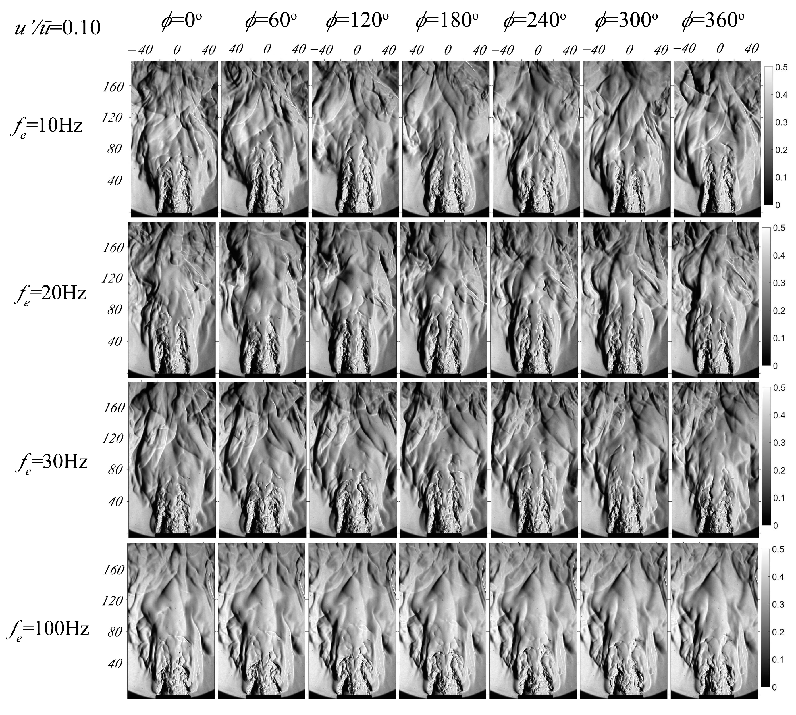
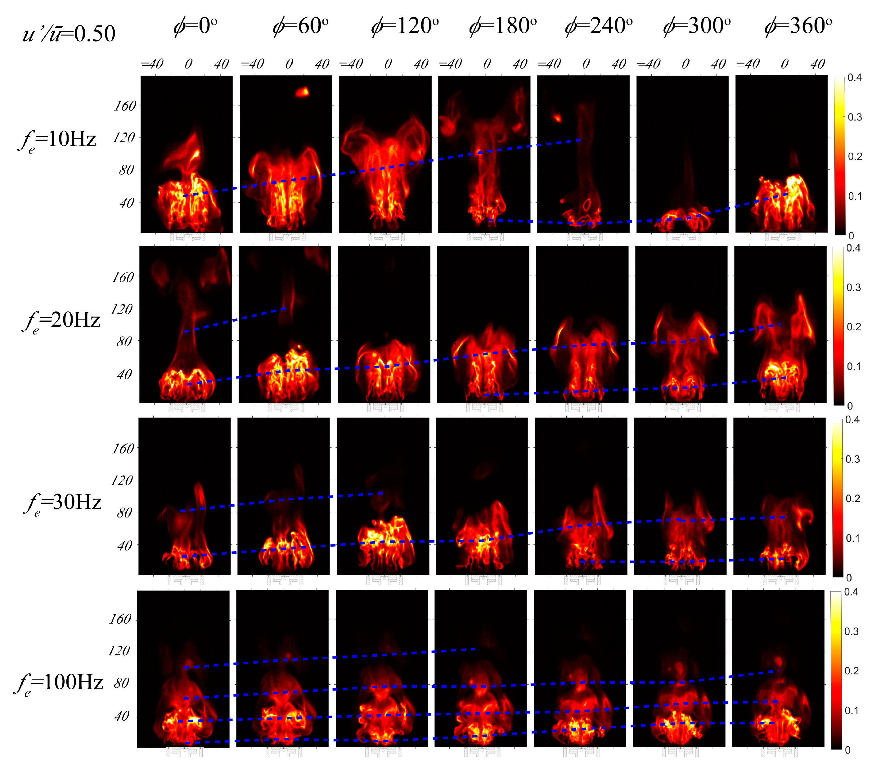
In this section, we processed a sequence of CH* chemiluminescence and schlieren images to reveal the interaction mechanism between flow and reaction. We analyzed the heat release response at four excitation frequencies: 10 Hz, 20 Hz, 30 Hz, and 100 Hz for u′/ū = 0.10 and 0.50. The 10 Hz case corresponds to the maximum gain of the FDF, whereas the 20 Hz and 30 Hz cases correspond to the local gain valley and peak, respectively. We also analyzed the response under relatively high-frequency excitations of 100 Hz. The instantaneous CH* chemiluminescence images and the corresponding schlieren images under excitation amplitudes of 0.10 and 0.50 are shown in Figure 8, Figure 9, Figure 10 and Figure 11. The phase angle of 0° corresponds to the maximum positive value of velocity fluctuation, while 180° corresponds to the minimum negative value of velocity fluctuations.
Under low-amplitude velocity excitation, flame height, and overall phase remain relatively constant within an excitation cycle, particularly at high frequencies. Because of the short high-frequency excitation period, the HRR distribution only causes local lift and curling at the nozzle exit, without affecting the downstream flame region. The flame dynamic is mainly characterized by the changes in the wrinkle of the flame sheet, which can be observed more prominently from a side view. The number of wrinkles increases with increasing excitation frequency. High excitation amplitudes result in significant changes to flame morphology, with distinct differences in change characteristics depending on excitation frequency. At a low-frequency excitation of 10 Hz, the flame undergoes multiple processes, including curling, bifurcation, overall extinguishment downstream, and gradual strengthening of the reaction upstream, as well as the formation of a vortex structure. In contrast, high-frequency excitation results in the formation of multiple distinct regions of heat release within a single cycle, with pronounced, vortex-like curling at their edges. Additionally, the main region of heat release increases in intensity from the nozzle and gradually decreases after reaching its maximum. The number of distinct regions of heat release increases as frequency increases. Specifically, a gradual transition between four layers of heat release regions was observed when the excited frequency was 100 Hz.
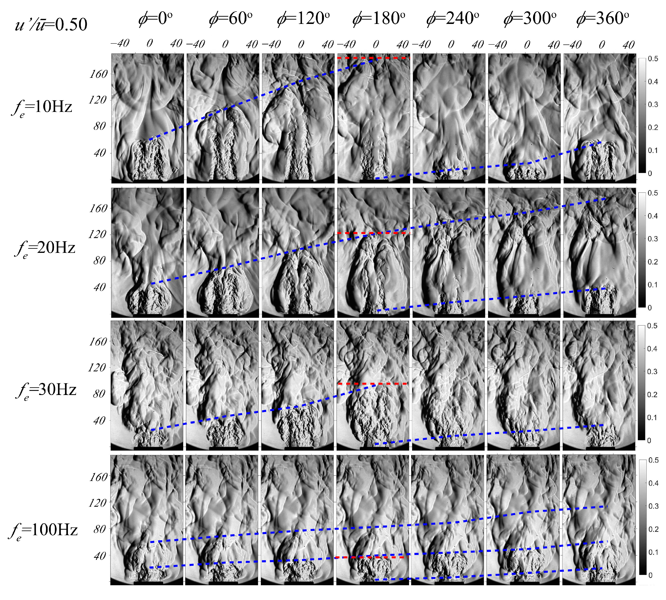
A clearly observable propagation process of large vortex structures induced by flow perturbation can be seen in the instantaneous schlieren images. The convective velocity of the disturbance mentioned earlier can be analyzed through schlieren images. The minimum excitation velocity corresponds to the phase of 180 degrees, which is also the origin of vortex structure formation. The height at which perturbations propagate downstream over a single excitation period is defined as the convective wavelength λf [50]. The convective wavelengths at different excitation frequencies and a fixed excitation amplitude of 0.5 are identified in Figure 11 with red lines. Meanwhile, the process of variation in the height of the large vortical structures is indicated by a green dashed line. The convective velocity of perturbations ucf can be calculated using the corresponding excitation frequency period τe and convective wavelength (ucf = λf/τe). The physical meaning of the ratio of flame length to convective wavelength (Lf/λf) is equivalent to the previously defined Stf. Hence, these two parameters were compared. The calculated convective wavelengths λf, convective velocity ucf, and Lf/λf for the four excitation frequencies are presented in Table 2. The results demonstrate an increase in convective velocity with increasing excitation frequency. The convective velocity is smaller than the jet velocity of 3.52 m/s with lower frequency excitation, and relatively higher frequency excitation results in a convective velocity close to the jet velocity. This variation may be linked to the flame length under different excitation frequencies. Specifically, under low-frequency forcing, the flame length exhibits a longer extent while the convective velocity experiences a decrease downstream of the flame. This convective velocity attenuation behavior has also been observed in premixed flames, as reported in references [46,51]. Consequently, such a variation of ucf causes significant deviations in Lf/λf and Stf at low-frequency conditions. Therefore, when analyzing the relationship between flame response and Stf, it is necessary to consider the changes in convective velocity.
4.5. Axial Distribution of Heat Release Oscillation
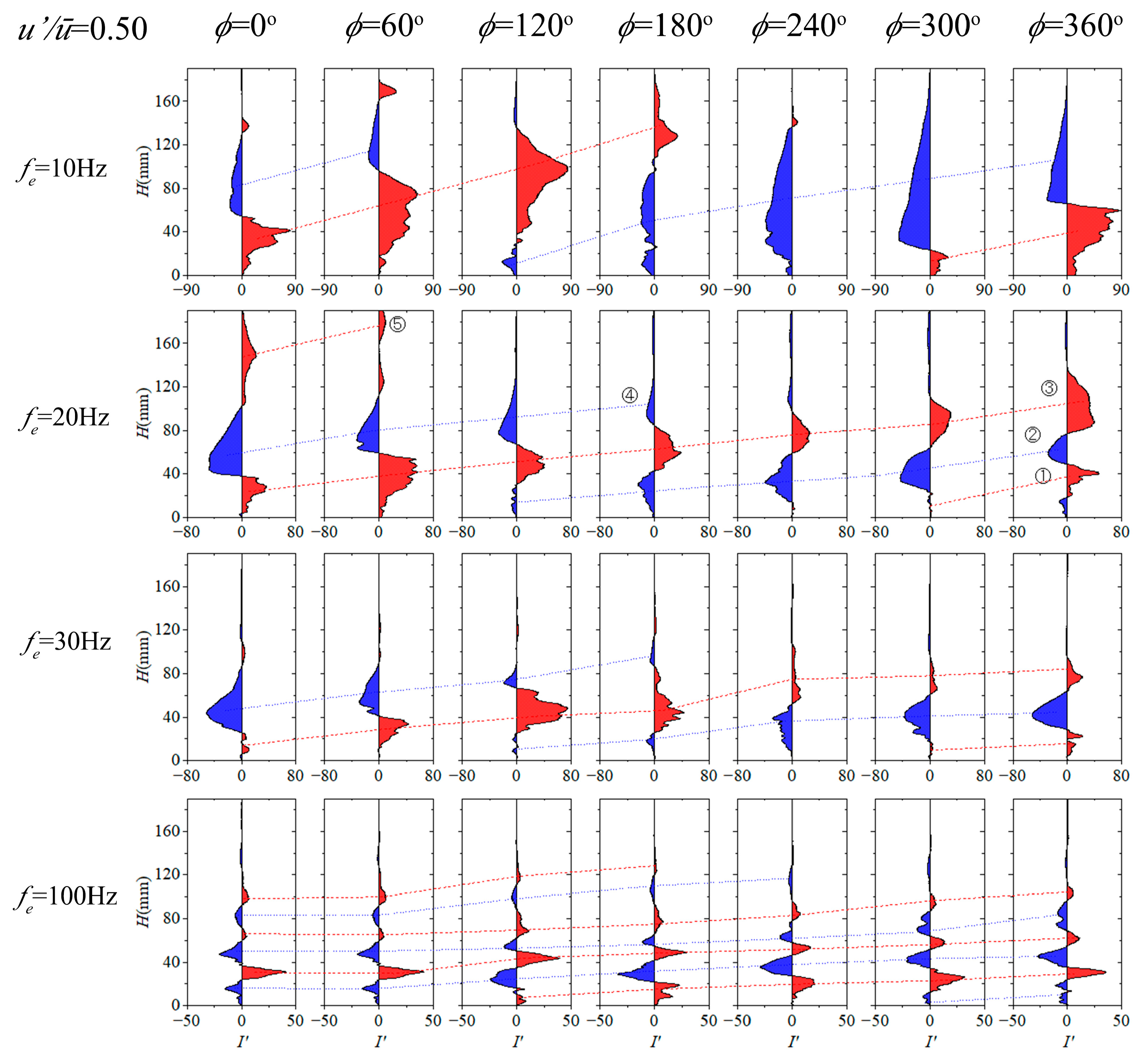
The axial distribution of heat release oscillations for various excitation frequencies is shown in Figure 12 at a velocity excitation amplitude of 0.50. Notably, distinct axial oscillation distributions are present for each different excitation frequency. At a low frequency of 10 Hz, the velocity excitation predominantly causes positive heat release oscillations upstream within the 0–180° phase range. Additionally, the positive oscillation region progressively diminishes and propagates downstream. After the 180-degree phase, when the excitation velocity reaches its minimum negative value, the entire middle and lower region begin to experience flameout. This results in a negative oscillation of heat release. Eventually, due to the increase in velocity fluctuation, the heat release in the upstream region increases, resulting in inducing positive oscillation and entering the next cycle. At 10 Hz excitation, positive or negative oscillations appear predominantly in the axial distribution of heat release, and the oscillation zones are relatively broad. Subsequently, the corresponding oscillation amplitude is also significant, and this behavior is associated with Stf < 1. This oscillation pattern reveals the primary reason for the large gain of the flame under low-frequency (10 Hz) excitation.
Under 20 Hz excitation, unlike 10 Hz, both positive and negative oscillation zones coexist at various phases. Furthermore, the amplitudes of these two zones are equal, leading to a relatively small total heat release fluctuation value. As a result, this is the main reason for the appearance of the gain valley around 20 Hz. Under 30 Hz excitation, there are two opposing oscillation regions, but their relative relationship is significantly different from 20 Hz excitation frequency. Specifically, regarding the middle forward oscillation region, the corresponding region for 30 Hz excitation reaches its maximum value at ϕ = 120° and then quickly decays, which causes single-region predominance for most phases. Similar to that seen under 10 Hz excitation, leads to the appearance of local gain peaks under 30 Hz excitation. With 100 Hz high-frequency excitation, multiple alternating oscillation regions appear. At different phase angles, the heat release oscillations have a wavenumber ranging from 2.0 to 2.5 within the flame length (Lf = 87.6 mm). This is consistent with the Stf (2.43) and the number of heat release layers (2–3) in Figure 10. Additionally, the oscillation amplitude of the downstream region decreases significantly relative to the upstream region. This multi-region alternating structure under high-frequency excitation means that positive and negative oscillations at the same moment have a counteractive effect, and thus the dispersed oscillation amplitude is relatively small, which leads to a relatively low gain under high-frequency excitation. This is the main reason for the low-pass filtering characteristic of the flame.
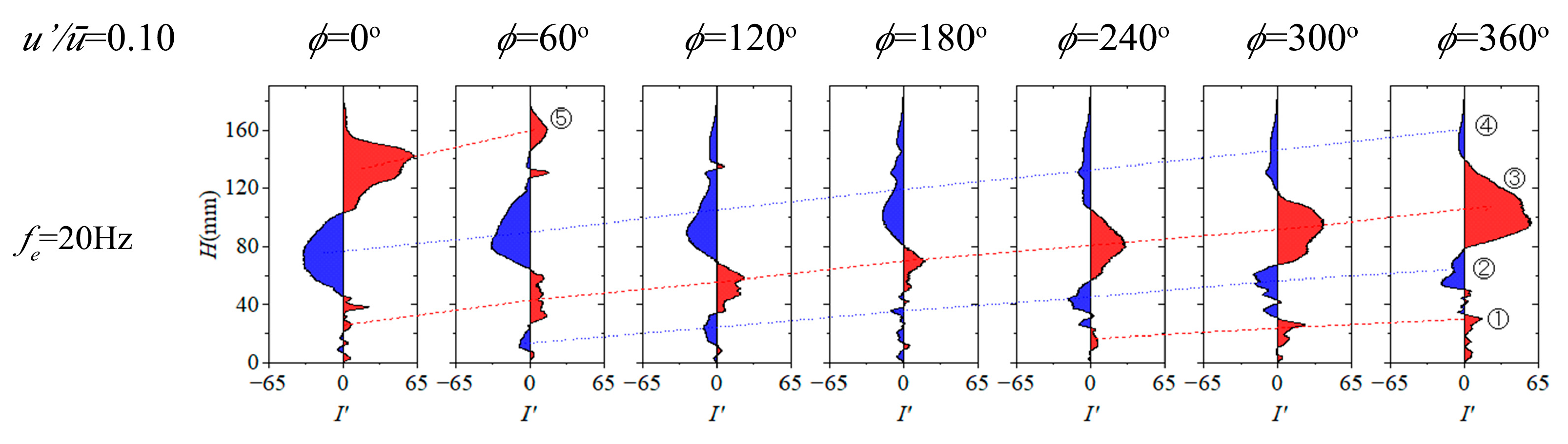
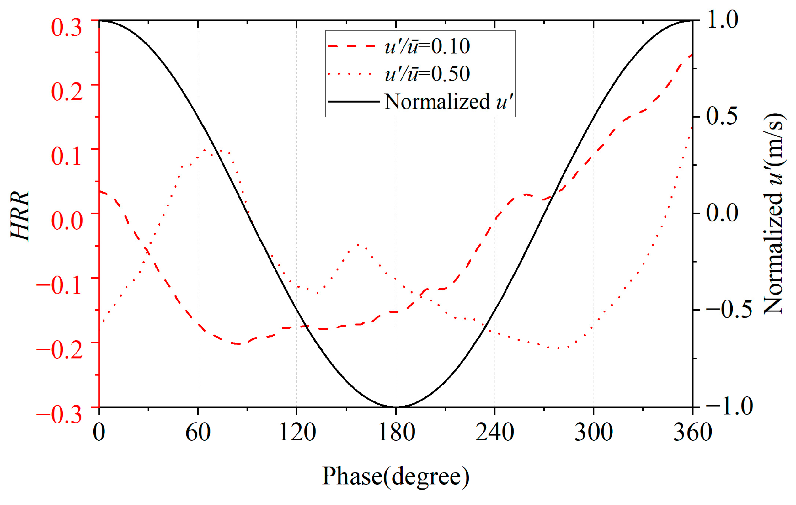
The phase-lag varies significantly at different excitation amplitudes at 20 Hz, presenting another noteworthy phenomenon. Therefore, we analyzed the axial distribution of heat release oscillation under the condition of 20 Hz and 0.1 excitation amplitude. As shown in Figure 13, comparing the two, we found that, although the number of axial regions is consistent under two different amplitudes, the variation trends of the five oscillation regions differ significantly, especially in the phase range of ϕ = 0~180°. The overall HRR oscillation and the normalized velocity fluctuation with different phase angles under excitation amplitudes of 0.1 and 0.5 are presented in Figure 14. Under a low-amplitude excitation (u′/ū = 0.10), the positive oscillation of region number 5 decreased noticeably, while the negative oscillation of region number 4 remained unchanged. As a result, there was a diminishing trend in HRR during phase interval of 0~120°. Following the 120° phase, a decline in the negative oscillation of region number 4 was observed while the positive oscillation of region number 3 intensified, leading to an early rise in HRR compared to the phase of velocity fluctuations. In contrast, when the excitation amplitude was high at 0.5, both the positive oscillation of region number 4 and the negative oscillation of region number 5 experienced attenuation. Meanwhile, the positive oscillation of region number 3 increased initially, decreased subsequently, and dominated the value after the 60° phase. As a result, the overall HRR first increased, then decreased within the phase range of 0 to 120°. After the 120° phase, the negative oscillation of region number 2 emerged and gradually intensified, causing a continued decrease in overall HRR until a phase angle of 300° was reached. At a phase angle of 360°, an increase in HRR was observed due to an increase in the positive oscillation of region number 3. Consequently, there was a delay of approximately 90° between the lowest HRR and the minimum velocity fluctuation.
The relative change trend of the oscillation region varies depending on different excitation amplitudes, resulting in a considerable phase difference. This shift is primarily due to the proximity of the positive and negative oscillation amplitude, causing the overall HRR to be more sensitive to variations within a single oscillation region. These conditions are susceptible to changes in the excitation frequency or amplitude, leading to considerable phase shifts.
5. Conclusions
This study experimentally investigates the nonlinear heat release response of a non-premixed methane–air flame to low-frequency acoustic excitations. The experiment measures the flame describing function (FDF) and analyzes the CH* chemiluminescence and schlieren images. It reveals the governing mechanisms of the nonlinear response. The FDF is characterized by low-pass filtering. When Stf > 3, the gain value is consistently below 0.25. The highest gain is observed at Stf = 0.43, and local valley and peak values of gain are observed at Stf ranges of 0.7–0.9 and 1.2–1.5, respectively. The local gain peaks and valleys of the FDF are related to the spatial distribution wavenumber of the heat release at different Stf values. As Stf increases, the oscillation zone of the flame shifts to higher wavenumbers, and the relative intensity of the positive and negative oscillation zones result in different cancellation effects. When the positive and negative oscillation zones are close to each other, the cancellation effect is at its maximum, leading to the minimum gain. In this condition, variations in frequency or amplitude can cause anomalous changes in the phase-lag of the flame, as the overall HRR becomes more sensitive to changes in a certain oscillation zone. Under relatively high-frequency excitation conditions, multiple oscillation zones of heat release along the flame are observed. The dispersion of multiple oscillation zones, as well as the cancellation effect of oscillation zones, are the primary causes of the low-pass filtering characteristic of the flame. The flame length significantly decreases under large amplitude and high-frequency excitation. Specifically, the normalized flame length (Lf/D) decreases from 3.79 to 2.37 when the excitation amplitude increases at an excitation frequency of 100 Hz. The delay time corresponding to the phase-lag exhibits the same as the convection time of disturbances under conditions of large-amplitude and high-frequency excitation. This behavior may be related to the accurate determination of the average convective velocity and the consistency of the oscillation region and the COM with short flame. These findings may provide insights into the stable design of non-premixed flame related to thermoacoustic instability.
Author Contributions
Conceptualization, T.Z. and D.P.; methodology, C.J.; investigation, D.P.; resources, T.Z.; data curation, D.P.; writing—original draft preparation, D.P.; writing—review and editing, D.P. and C.J.; visualization, D.P.; supervision, T.Z.; funding acquisition, T.Z. All authors have read and agreed to the published version of the manuscript.
Funding
This research was funded by National Natural Science Foundation of China, grant number 51976140, and Science and Technology Commission of Shanghai Municipality, grant number 20DZ1204902.
Institutional Review Board Statement
Not applicable.
Informed Consent Statement
Not applicable.
Data Availability Statement
Not applicable.
Conflicts of Interest
The authors declare no conflict of interest.
References
- Acharya, V.S.; Bothien, M.R.; Lieuwen, T.C. Non-Linear Dynamics of Thermoacoustic Eigen-Mode Interactions. Combust. Flame 2018, 194, 309–321. [Google Scholar] [CrossRef]
- Shreekrishna; Hemchandra, S.; Lieuwen, T. Premixed Flame Response to Equivalence Ratio Perturbations. Combust. Theory Model. 2010, 14, 681–714. [Google Scholar] [CrossRef]
- O’Connor, J.; Vanatta, C.; Mannino, J.; Lieuwen, T. Mechanisms for Flame Response in a Transversely Forced Flame. In Proceedings of the 7th US National Technical Meeting of the Combustion Institute, Atlanta, GA, USA, 20–23 March 2011. [Google Scholar]
- Preetham, S.H.; Lieuwen, T.C. Response of Turbulent Premixed Flames to Harmonic Acoustic Forcing. Proc. Combust. Inst. 2007, 31, 1427–1434. [Google Scholar] [CrossRef]
- Durox, D. Theoretical and Experimental Determinations of the Transfer Function of a Laminar Premixed Flame. Proc. Combust. Inst. 2000, 28, 765–773. [Google Scholar]
- Fleifil, M.; Annaswamy, A.M.; Ghoneim, Z.A.; Ghoniem, A.F. Response of a Laminar Premixed Flame to Flow Oscillations: A Kinematic Model and Thermoacoustic Instability Results. Combust. Flame 1996, 106, 487–510. [Google Scholar] [CrossRef]
- Merk, M.; Gaudron, R.; Silva, C.; Gatti, M.; Mirat, C.; Schuller, T.; Polifke, W. Prediction of Combustion Noise of an Enclosed Flame by Simultaneous Identification of Noise Source and Flame Dynamics. Proc. Combust. Inst. 2019, 37, 5263–5270. [Google Scholar] [CrossRef]
- Boudy, F.; Schuller, T.; Durox, D.; Candel, S. The Flame Describing Function (FDF) Unified Framework for Combustion Instability Analysis: Progress and Limitations. In Proceedings of the International Workshop on Non-Normal and Nonlinear Effects in Aero- and Thermo-Acoustics, Munich, Germany, 18–21 June 2013. [Google Scholar]
- Dowling, A.P. Nonlinear Self-Excited Oscillations of a Ducted Flame. J. Fluid Mech. 1997, 346, 271–290. [Google Scholar] [CrossRef]
- Noiray, N.; Durox, D.; Schuller, T.; Candel, S. A Unified Framework for Nonlinear Combustion Instability Analysis Based on the Flame Describing Function. J. Fluid Mech. 2008, 615, 139–167. [Google Scholar] [CrossRef]
- Krediet, H.J.; Beck, C.H.; Krebs, W.; Schimek, S.; Paschereit, C.O.; Kok, J.B.W. Identification of the Flame Describing Function of a Premixed Swirl Flame from LES. Combust. Sci. Technol. 2012, 184, 888–900. [Google Scholar] [CrossRef]
- Tay-Wo-Chong, L.; Bomberg, S.; Ulhaq, A.; Komarek, T.; Polifke, W. Comparative Validation Study on Identification of Premixed Flame Transfer Function. J. Eng. Gas Turbines Power 2012, 134, 021502. [Google Scholar] [CrossRef]
- Kim, K.T.; Lee, H.J.; Lee, J.G.; Quay, B.D.; Santavicca, D. Flame Transfer Function Measurement and Instability Frequency Prediction Using a Thermoacoustic Model. In Proceedings of the ASME Turbo Expo, Orlando, FL, USA, 8–12 June 2009. [Google Scholar]
- Alemela, P.R.; Fanca, D.; Ettner, F.; Hirsch, C.; Sattelmayer, T.; Schuermans, B. Flame Transfer Matrices of a Premixed Flame and a Global Check with Modelling and Experiments. In Proceedings of the ASME Turbo Expo, Berlin, Germany, 9–13 June 2008. [Google Scholar]
- Gaudron, R.; Gatti, M.; Mirat, C.; Schuller, T. Impact of the Injector Size on the Transfer Functions of Premixed Laminar Conical Flames. Combust. Flame 2017, 179, 138–153. [Google Scholar] [CrossRef]
- Schuller, T.; Durox, D.; Candel, S. A Unified Model for the Prediction of Laminar Flame Transfer Functions: Comparisons between Conical and V-Flame Dynamics. Combust. Flame 2003, 134, 21–34. [Google Scholar] [CrossRef]
- Boudy, F.; Durox, D.; Schuller, T.; Candel, S. Nonlinear Mode Triggering in a Multiple Flame Combustor. Proc. Combust. Inst. 2011, 33, 1121–1128. [Google Scholar] [CrossRef]
- Hermeth, S.; Staffelbach, G.; Gicquel, L.Y.M.; Anisimov, V.; Cirigliano, C.; Poinsot, T. Bistable Swirled Flames and Influence on Flame Transfer Functions. Combust. Flame 2014, 161, 184–196. [Google Scholar] [CrossRef]
- Ćosić, B.; Terhaar, S.; Moeck, J.P.; Paschereit, C.O. Response of a Swirl-Stabilized Flame to Simultaneous Perturbations in Equivalence Ratio and Velocity at High Oscillation Amplitudes. Combust. Flame 2015, 162, 1046–1062. [Google Scholar] [CrossRef]
- Palies, P.; Durox, D.; Schuller, T.; Candel, S. Experimental Study on the Effect of Swirler Geometry and Swirl Number on Flame Describing Functions. Combust. Sci. Technol. 2011, 183, 704–717. [Google Scholar] [CrossRef]
- Shanbhogue, S.; Shin, D.; Hemchandra, S.; Plaks, D.; Lieuwen, T. Flame Sheet Dynamics of Bluff-Body Stabilized Flames during Longitudinal Acoustic Forcing. Proc. Combust. Inst. 2009, 32, 1787–1794. [Google Scholar] [CrossRef]
- Schuermans, B.; Bellucci, V.; Flohr, P.; Paschereit, C.O. Thermoacoustic Flame Transfer Function of a Gas Turbine Burner in Premix and Pre- Premix Combustion. In Proceedings of the AIAA Aerospace Sciences Meeting and Exhibit, Reno, NV, USA, 5–8 January 2004. [Google Scholar]
- Kim, K.T.; Santavicca, D.A. Generalization of Turbulent Swirl Flame Transfer Functions in Gas Turbine Combustors. Combust. Sci. Technol. 2013, 185, 999–1015. [Google Scholar] [CrossRef]
- Kim, K.T.; Lee, J.G.; Quay, B.D.; Santavicca, D.A. Spatially Distributed Flame Transfer Functions for Predicting Combustion Dynamics in Lean Premixed Gas Turbine Combustors. Combust. Flame 2010, 157, 1718–1730. [Google Scholar] [CrossRef]
- Tyagi, M.; Chakravarthy, S.R.; Sujith, R.I. Unsteady Combustion Response of a Ducted Non-Premixed Flame and Acoustic Coupling. Combust. Theory Model. 2007, 11, 205–226. [Google Scholar] [CrossRef]
- Chandrasekhar, S.V.; Chakravarthy, S.R. Response of Non-Premixed Ducted Flame to Transverse Oscillations and Longitudinal Acoustic Coupling. In Proceedings of the 43rd AIAA/ASME/SAE/ASEE Joint Propulsion Conference, Cincinnati, OH, USA, 8–11 July 2007. [Google Scholar]
- Magina, N.; Acharya, V.; Lieuwen, T. Forced Response of Laminar Non-Premixed Jet Flames. Prog. Energy Combust. Sci. 2019, 70, 89–118. [Google Scholar] [CrossRef]
- Magina, N.; Shin, D.H.; Acharya, V.; Lieuwen, T. Response of Non-Premixed Flames to Bulk Flow Perturbations. Proc. Combust. Inst. 2013, 34, 963–971. [Google Scholar] [CrossRef]
- Lieuwen, T.C. Unsteady Combustor Physics, 1st ed.; Cambridge University Press: New York, NY, USA, 2012; pp. 364–369. [Google Scholar]
- Yao, Z.; Zhu, M. A Distributed Transfer Function for Non-Premixed Combustion Oscillations. Combust. Sci. Technol. 2012, 184, 767–790. [Google Scholar] [CrossRef]
- Jiang, J.; Jing, L.; Zhu, M.; Jiang, X. A Comparative Study of Instabilities in Forced Reacting Plumes of Nonpremixed Flames. J. Energy Inst. 2016, 89, 456–467. [Google Scholar] [CrossRef]
- Farhat, S.; Kleiner, D.; Zhang, Y. Jet Diffusion Flame Characteristics in a Loudspeaker-Induced Standing Wave. Combust. Flame 2005, 142, 317–323. [Google Scholar] [CrossRef]
- Farhat, S.A.; Ng, W.B.; Zhang, Y. Chemiluminescent Emission Measurement of a Diffusion Flame Jet in a Loudspeaker Induced Standing Wave. Fuel 2005, 84, 1760–1767. [Google Scholar] [CrossRef]
- Chen, L.W.; Wang, Q.; Zhang, Y. Flow Characterisation of Diffusion Flame in a Standing Wave. Exp. Therm. Fluid Sci. 2012, 41, 84–93. [Google Scholar] [CrossRef]
- Chen, L.W.; Wang, Q.; Zhang, Y. Flow Characterisation of Diffusion Flame under Non-Resonant Acoustic Excitation. Exp. Therm. Fluid Sci. 2013, 45, 227–233. [Google Scholar] [CrossRef]
- Sun, Y.; Zhao, D.; Ni, S.; David, T.; Zhang, Y. Entropy and Flame Transfer Function Analysis of a Hydrogen-Fueled Diffusion Flame in a Longitudinal Combustor. Energy 2020, 194, 116870. [Google Scholar] [CrossRef]
- Kim, T.; Ahn, M.; Lim, D.; Yoon, Y. Flame Describing Function and Combustion Instability Analysis of Non-Premixed Coaxial Jet Flames. Exp. Therm. Fluid Sci. 2022, 136, 110642. [Google Scholar] [CrossRef]
- Fu, X.; Yang, F.; Guo, Z. Combustion Instability of Pilot Flame in a Pilot Bluff Body Stabilized Combustor. Chin. J. Aeronaut. 2015, 28, 1606–1615. [Google Scholar] [CrossRef]
- Ahn, B.; Lee, J.; Jung, S.; Kim, K.T. Low-Frequency Combustion Instabilities of an Airblast Swirl Injector in a Liquid-Fuel Combustor. Combust. Flame 2018, 196, 424–438. [Google Scholar] [CrossRef]
- Chen, Y.C.; Chang, C.C.; Pan, K.L.; Yang, J.T. Flame Lift-off and Stabilization Mechanisms of Nonpremixed Jet Flames on a Bluff-Body Burner. Combust. Flame 1998, 115, 51–65. [Google Scholar] [CrossRef]
- Hardalupas, Y.; Selbach, A. Imposed Oscillations and Non-Premixed Flames. Prog. Energy Combust. Sci. 2002, 28, 75–104. [Google Scholar] [CrossRef]
- Putnam, A.A. Combustion Roar as Observed in Industrial Furnaces. J. Eng. Power 1982, 104, 867–873. [Google Scholar] [CrossRef]
- Putnam, A.; Faulkner, L. An Overview of Combustion Noise. J. Energy 1983, 7, 458–469. [Google Scholar] [CrossRef]
- Chung, J.Y.; Blaser, D.A. Transfer Function Method of Measuring In-Duct Acoustic Properties. I. Theory. J. Acoust. Soc. Am. 1980, 68, 907–913. [Google Scholar] [CrossRef]
- Balachandran, R.; Ayoola, B.O.; Kaminski, C.F.; Dowling, A.P.; Mastorakos, E. Experimental Investigation of the Nonlinear Response of Turbulent Premixed Flames to Imposed Inlet Velocity Oscillations. Combust. Flame 2005, 143, 37–55. [Google Scholar] [CrossRef]
- Kim, D.; Lee, J.G.; Quay, B.D.; Santavicca, D.A.; Kim, K.; Srinivasan, S. Effect of Flame Structure on the Flame Transfer Function in a Premixed Gas Turbine Combustor. J. Eng. Gas Turbines Power 2010, 132, 021502. [Google Scholar] [CrossRef]
- Ranalli, J.A.; Ferguson, D.; Martin, C. Simple Analysis of Flame Dynamics via Flexible Convected Disturbance Models. J. Propuls. Power 2012, 28, 1268–1276. [Google Scholar] [CrossRef]
- Szedlmayer, M.T.; Quay, B.D.; Samarasinghe, J.; De Rosa, A.; Lee, J.G.; Santavicca, D.A. Forced Flame Response of a Lean Premixed Multi-Nozzle Can Combustor. In Proceedings of the ASME Turbo Expo, Vancouver, BC, Canada, 6–10 June 2011. [Google Scholar]
- Jones, B.; Lee, J.G.; Quay, B.D.; Santavicca, D.A. Flame Response Mechanisms Due to Velocity Perturbations in a Lean Premixed Gas Turbine Combustor. J. Eng. Gas Turbines Power 2011, 133, 021503. [Google Scholar] [CrossRef]
- Shin, D.H.; Lieuwen, T. Flame Wrinkle Destruction Processes in Harmonically Forced, Turbulent Premixed Flames. J. Fluid Mech. 2013, 721, 484–513. [Google Scholar] [CrossRef]
- Liu, W.; Xue, R.; Zhang, L.; Yang, Q.; Wang, H. Nonlinear Response of a Premixed Low-Swirl Flame to Acoustic Excitation with Large Amplitude. Combust. Flame 2022, 235, 111733. [Google Scholar] [CrossRef]
Figure 1.
Schematic of the experimental setup. Unit: mm.

Figure 2.
Schematic diagram of flame length and the height of COM. Lf represents the flame length, while Pfy represents the height of COM.
Figure 2.
Schematic diagram of flame length and the height of COM. Lf represents the flame length, while Pfy represents the height of COM.

Figure 3.
Measured flame describing function: (a) The evolution of the gain with excitation frequency at different excitation amplitudes; (b) The evolution of the phase-lag with excitation frequency at different excitation amplitudes.
Figure 3.
Measured flame describing function: (a) The evolution of the gain with excitation frequency at different excitation amplitudes; (b) The evolution of the phase-lag with excitation frequency at different excitation amplitudes.

Figure 4.
The time-averaged distributions of CH* chemiluminescence with different excitation frequencies and amplitudes.
Figure 4.
The time-averaged distributions of CH* chemiluminescence with different excitation frequencies and amplitudes.

Figure 5.
The time-averaged flame length (Lf) and height of the COM (Pfy) with different excitation frequencies and amplitudes.
Figure 5.
The time-averaged flame length (Lf) and height of the COM (Pfy) with different excitation frequencies and amplitudes.

Figure 6.
The calculated Stf and the generated FDF: (a) The evolution of the stf with the excitation frequency; (b) The generated gain of the FDF with Stf.
Figure 6.
The calculated Stf and the generated FDF: (a) The evolution of the stf with the excitation frequency; (b) The generated gain of the FDF with Stf.

Figure 7.
The comparison of time delay and convection time under different excitation frequencies and amplitude: (a) The time delay calculated through the phase-lag. The red frame in the picture highlights the anomalous time delay associated with 20Hz excitations. (b) The convection time calculated through the height of the COM and the constant convective velocity (ucv = 3.52 m/s).

Figure 8.
The instantaneous CH* chemiluminescence images in an excitation cycle at different excitation frequencies with u′/ū = 0.10.
Figure 8.
The instantaneous CH* chemiluminescence images in an excitation cycle at different excitation frequencies with u′/ū = 0.10.

Figure 9.
The instantaneous schlieren images in an excitation cycle at different excitation frequencies with u′/ū = 0.10.
Figure 9.
The instantaneous schlieren images in an excitation cycle at different excitation frequencies with u′/ū = 0.10.

Figure 10.
The instantaneous CH* chemiluminescence images in an excitation cycle at different excitation frequencies with u′/ū = 0.50.
Figure 10.
The instantaneous CH* chemiluminescence images in an excitation cycle at different excitation frequencies with u′/ū = 0.50.

Figure 11.
The instantaneous schlieren images in an excitation cycle at different excitation frequencies with u′/ū = 0.50.
Figure 11.
The instantaneous schlieren images in an excitation cycle at different excitation frequencies with u′/ū = 0.50.

Figure 12.
The axial distribution of heat release oscillations with variation of phase angles at different excitation frequencies and u′/ū = 0.10. The red region in the graph represents the positive value zone, while the blue region represents the negative value zone.
Figure 12.
The axial distribution of heat release oscillations with variation of phase angles at different excitation frequencies and u′/ū = 0.10. The red region in the graph represents the positive value zone, while the blue region represents the negative value zone.

Figure 13.
The axial distribution of heat release oscillation with variation of phase angles at fe = 20 Hz and u′/ū = 0.10.
Figure 13.
The axial distribution of heat release oscillation with variation of phase angles at fe = 20 Hz and u′/ū = 0.10.

Figure 14.
The evolution of the HRR and the normalized velocity fluctuation with respect to the phase angle at two different excitation amplitudes, namely 0.10 and 0.50, at an excitation frequency of 20 Hz.
Figure 14.
The evolution of the HRR and the normalized velocity fluctuation with respect to the phase angle at two different excitation amplitudes, namely 0.10 and 0.50, at an excitation frequency of 20 Hz.


Table 1.
The operating conditions for the burner and acoustic excitations.
| Parameters | Values |
|---|---|
| Gas flow rate (Nm3/h) | 0.42 |
| Air flow rate (Nm3/h) | 4.67 |
| Air velocity in the ring, u0 (m/s) | 3.52 |
| Air velocity before the nozzle, ū (m/s) | 1.40 |
| gas velocity at the nozzle, ugas (m/s) | 4.10 |
| Equivalence ratio | 0.86 |
| Excitation frequency, fe (Hz) | 10, 15, 20, 25, 30, 35, 45, 50, 60, 70, 80, 90, 100, 120 |
| Excitation amplitude, u′/ū | 0.10, 0.20, 0.30, 0.40, 0.50 |
Table 2.
The calculated parameters related to convective velocity ucf.
| fe (Hz) | 10 | 20 | 30 | 100 |
| λf (mm) | 190.4 | 121.7 | 87.6 | 30.9 |
| τe (s) | 0.100 | 0.050 | 0.033 | 0.010 |
| Lf (mm) | 152.4 | 161.2 | 113.6 | 87.6 |
| ucf (m/s) | 1.90 | 2.43 | 2.63 | 3.61 |
| Lf/λf | 0.80 | 1.32 | 1.29 | 2.42 |
| Stf | 0.43 | 0.92 | 0.97 | 2.43 |
Disclaimer/Publisher’s Note: The statements, opinions and data contained in all publications are solely those of the individual author(s) and contributor(s) and not of MDPI and/or the editor(s). MDPI and/or the editor(s) disclaim responsibility for any injury to people or property resulting from any ideas, methods, instructions or products referred to in the content. |
© 2023 by the authors. Licensee MDPI, Basel, Switzerland. This article is an open access article distributed under the terms and conditions of the Creative Commons Attribution (CC BY) license (https://creativecommons.org/licenses/by/4.0/).
Share and Cite
MDPI and ACS Style
Pan, D.; Ji, C.; Zhu, T. Characterization of Nonlinear Responses of Non-Premixed Flames to Low-Frequency Acoustic Excitations. Appl. Sci. 2023, 13, 6237. https://doi.org/10.3390/app13106237
AMA Style
Pan D, Ji C, Zhu T. Characterization of Nonlinear Responses of Non-Premixed Flames to Low-Frequency Acoustic Excitations. Applied Sciences. 2023; 13(10):6237. https://doi.org/10.3390/app13106237
Chicago/Turabian StylePan, Deng, Chenzhen Ji, and Tong Zhu. 2023. "Characterization of Nonlinear Responses of Non-Premixed Flames to Low-Frequency Acoustic Excitations" Applied Sciences 13, no. 10: 6237. https://doi.org/10.3390/app13106237
Note that from the first issue of 2016, this journal uses article numbers instead of page numbers. See further details here.