Identification of the Constitutive Parameters of Viscosity and the Prediction of the Cutting Force of S32760 Duplex Stainless Steel under a High Strain Rate

Abstract

The mechanical properties of S32760 duplex stainless steel under dynamic loading conditions at high strain rates are significantly different from those under quasi-static conditions. As a result of large strain, high strain rate, and high temperature, the analysis of the cutting process needs to factor in the influence of the viscous behavior of the material on the plastic deformation process. Based on the viscous effect of the two phases and the mixing rule, a mechanical threshold stress (MTS) constitutive model of S32760 duplex stainless steel considering the viscous effect is established to analyze the effect of strain rate on flow stress. An inverse identification method of the constitutive parameters based on Oxley's theory is proposed. The constitutive parameters of S32760 duplex stainless steel were reversely modified using an equal shear zone model and an orthogonal cutting experiment. The results show that the viscosity of the austenite phase was greater than that of the ferrite phase, and the strain rate had the greatest influence on the viscosity effect in the constitutive model. The prediction error of the constitutive model constructed in this manuscript was less than 4%, which had high accuracy.

1. Introduction

Duplex stainless steel is a kind of steel that contains both austenite and ferrite phases in its metallographic structure. The two-phase structure exists independently. By correctly controlling the chemical composition and heat treatment process, duplex stainless steel can have the advantages of both ferritic stainless steel and austenitic stainless steel. These steels have been widely used in petroleum and chemical industries, military applications, the paper industry, and other fields [1].

From the perspective of material deformation, the properties of materials at different strain rates are different, as also the dominant characteristics of materials during deformation. In the process of gradually increasing from a low strain rate to a high strain rate, the degree of the deformation of the material gradually increases in severity. The material undergoes a transition from static deformation to dynamic deformation and also undergoes a transition from elastic deformation to plastic deformation. The plastic deformation of the material is divided into two stages as the strain rate increases. While the first stage only depends on the elasticity or plasticity of the material, the second stage depends on the viscosity of the material [2]. Material viscosity is generally employed to describe the relationship between fluid stress and the strain rate, which is manifested as the strain rate effect. The greater the viscosity, the more obvious the strain rate effect of the material [3]. Behera et al. [4] explored the flow stress of 416 martensitic stainless steel with a strain rate from 10⁻³ s⁻¹ to 1.5 × 10³ s⁻¹ by employing a universal testing machine and the Hopkinson pressure bar experiment. The results indicated that 416 martensitic stainless steel exhibits strain rate sensitivity.

With large plastic deformation, the cutting strain rate increases with an increase in the cutting speed, reaching the order of 10⁴ s⁻¹ [5] in high-speed cutting. Based on finite element simulations, a numerical model of the turning process of corrosion-resistant nickel-based alloy-X was established by Çakır et al. [6]. The results showed that the cutting force could be reduced by increasing the cutting speed and reducing the feed rate. The cutting temperature increases with an increase in the cutting speed and feed rate. Based on finite element simulations, an ultrasonic-assisted turning method using Ti6Al4V alloy was established by Çakır et al. [7]. The results show that ultrasonic-assisted turning reduces the cutting force and cutting temperature and improves tool life. In engineering applications, selecting the appropriate constitutive relationship to describe the mechanical behavior of materials is the prerequisite for the bearing and failure analysis of engineering structures. Wang Qiang et al. [8] reviewed the latest research progress on metal thermoviscoplastic constitutive relations and introduced and discussed several common metal thermoviscoplastic constitutive relations in detail. The Zerilli–Armstrong (Z–A) [9] constitutive model can well represent the deformation characteristics of dual-phase materials and is also a commonly used constitutive model in composite materials. However, in this study, we used the constitutive model to simulate the cutting process. The Z–A constitutive model has a high degree of agreement with the flow stress at low strain rates. However, when the strain rate exceeds 10⁴ s⁻¹, the actual flow stress greatly deviates from the constitutive model simulation. The Steinberg–Guina (S–G) [10] constitutive model can perform well in cutting simulations within the range of the strain rate in the Hopkinson pressure bar experiment, and the data are in good agreement. However, once the strain rate is exceeded, it will cause a large deviation in the simulation results, similar to the Z–A constitutive model. The MTS [11] constitutive model can accurately reflect the change in the flow stress of the material at a high strain rate and can well express the plastic deformation coupling mechanism of the two-phase material. The only drawback is that the model lacks the viscous effect. If the model is modified, and the viscous effect is taken into account, the cutting process of the dual-phase material will be better simulated.

There are two main methods to obtain constitutive parameters: the finite element method and the Hopkinson pressure bar experiment. Zhang Bin et al. [12] proposed a hybrid strategy to determine the constitutive parameters for thin-walled tubes based on experimental responses from hydraulic bulge tests. The method integrates analytical models, finite element analysis, and gradient-based optimization algorithms. Shrot et al. [13] proposed a finite element identification method for parameters based on the Levenberg–Marquardt search algorithm. Although this method can be used to develop the constitutive equation for the material, it requires a lot of calculation and is time-consuming. The Hopkinson pressure bar experiment is the most direct method to obtain the parameters. Several studies have developed constitutive equations for different materials using the Hopkinson pressure bar experiment [14]. He Muyang et al. [15] determined the parameters of the 11MnNiMo constitutive model by adopting the Hopkinson pressure bar experiment. However, this method can only be used to study the behavior of the metal at a strain rate of 10³~10⁴ s⁻¹.

The existing parameter acquisition methods are difficult to apply in identifying the viscous behavior of materials under high strain rate conditions in the cutting process. It is also difficult to ensure the reliability of test data and the adaptability of test conditions. Therefore, in view of the above problems, we analyze the viscous effect of duplex stainless steel under high strain rate conditions and establish the MTS constitutive equation for S32760 duplex stainless steel based on the viscous effect of the two phases and the mixing rule. A reverse identification method for parameters based on a cutting theory suitable for high strain rate conditions is also proposed. Based on the characteristics of the ferrite and austenite phases of S32760, the theoretical range of the undetermined parameters of the S32760 two-phase constitutive model is determined, and a model of equal shear zones in orthogonal cutting is established. Based on the results of the metal cutting trials, the constitutive parameters of S32760 duplex stainless steel are modified, and the viscous behavior of duplex stainless steel under a high strain rate is analyzed.

In this paper, the equal shear zone model of orthogonal cutting is established based on Oxley’s theory, and then the improved MTS constitutive model is established. Based on the principle of the least-square method and genetic algorithm, the constitutive parameters are preliminarily identified. The constitutive equation is used in the shear zone model to extract parameters such as strain and strain rate. Combined with the cutting force determined in the orthogonal cutting experiment, the constitutive parameters are inversely identified and corrected. The modified constitutive equation is then used in the shear zone model to predict the cutting force, and the results are compared with the cutting experimental data to verify the accuracy of the model. The constitutive model proposed in this manuscript can lay a theoretical foundation for the study of grain size and microhardness of machined surfaces and provide a theoretical basis for the optimization of cutting process parameters in the production of duplex stainless steel.

2. Equipartition Shear Zone Model of Orthogonal Cutting Based on Oxley’s Theory

In the cutting process, the plastic deformation of the material mainly occurs in the shear zone. Due to the increased cutting speed, the temperature in the shear zone sharply increases, which causes the thermal softening of the material, and thus the material undergoes greater plastic deformation. During the cutting process (especially high-speed cutting), the material exceeds its yield limit and flows like a fluid on the material matrix and the surface of the tool rake in the form of chips. Whether from the model or the actual processing, the cutting process is a viscous flow process similar to that of a fluid. A flow stress model of duplex stainless steel is closer to Newtonian fluid in terms of the viscous effect of materials.

Based on the experimental observation of material deformation in the shear zone, Oxley [16] established a theoretical relationship between the variables of the orthogonal cutting process (material properties, tool geometry, and cutting conditions) and output variables under the assumption of the plane strain and steady cutting conditions. The output variables of basic cutting characteristics such as temperature, chip geometry, and cutting force in the metal cutting deformation zone can be theoretically calculated. Based on Oxley’s predictive machining theory, the orthogonal cutting-force prediction model of S32760 duplex stainless steel is established herein.

2.1. Shear Zone Analysis

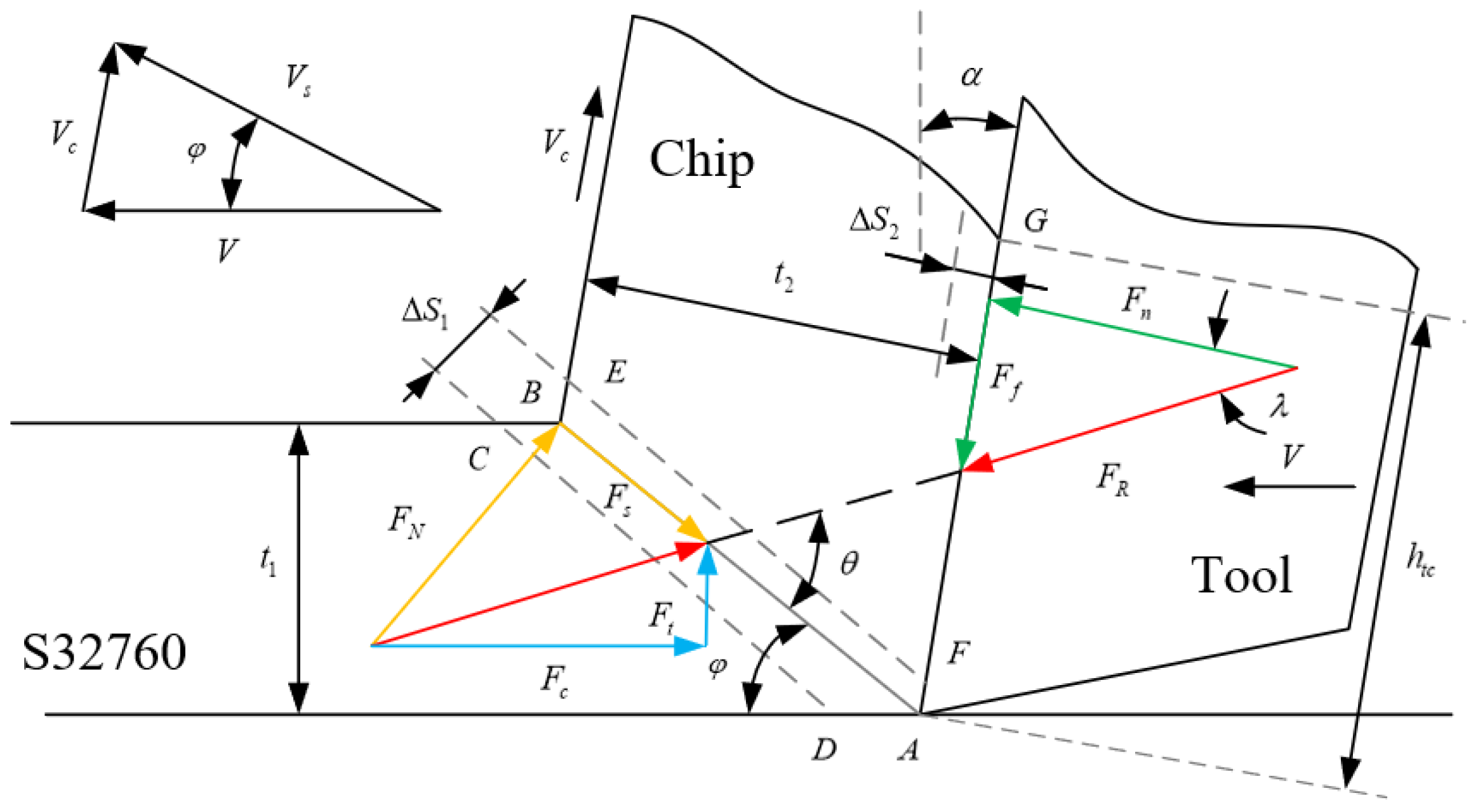
The schematic diagram of the orthogonal cutting shear zone is shown in Figure 1. A pair of equilibrium forces is formed by the normal force $F_N$ at the shear plane and the cutting force $F_s$ at the shear plane along with the normal force $F_n$ at the tool–chip interface and the friction force $F_f$ at the tool–chip interface. The chip formation force $F_R$ is decomposed into $F_c$ and $F_t$. The cutting-force components and the chip thickness $t_2$ can be calculated using the following formula:

$$F_c=F_R\cos (\lambda -\alpha )$$

(1)

$$F_t=F_R\sin (\lambda -\alpha )$$

(2)

$$F_f=F_R\sin \lambda$$

(3)

$$F_n=F_R\cos \lambda$$

(4)

$$F_R=\frac{F_s}{\cos \theta }=\frac{{\sigma }_{AB}{t}_{1}w}{\sin \phi \cos \theta }$$

(5)

$$t_2=t_1\cos (\phi -\alpha )/\sin \phi$$

(6)

where $\alpha$ is the rake angle of the tool; $\phi$ is the shear angle; $\lambda$ is the friction angle; $t_1$ is the undeformed chip thickness; $w$ is the cutting width; $\theta$ is the angle between $F_R$ and AB; ${\sigma }_{AB}$ represents the average flow stress on the AB plane.

In the Oxley model, there is a relationship between the velocity of any particle in the first deformation zone and the average shear strain rate in the shear zone expressed as follows:

$${\dot{\gamma }}_{avg}=\frac{V\cos \alpha }{\Delta S_1\cos (\phi -\alpha )}$$

(7)

where $V$ is the orthogonal cutting speed, and $\Delta S_1$ is the thickness between two parallel bands in the shear zone.

After the shear angle $\phi$ is determined, the strain and strain rate at any position on the shear plane can be obtained using the von Mises stress yield criterion.

$${\epsilon }_{AB}=\frac{1}{2\sqrt{3}}\cdot \frac{\cos \alpha }{\sin \phi \cos (\phi -\alpha )}$$

(8)

$${\dot{\epsilon }}_{AB}=\frac{1}{\sqrt{3}}\cdot \frac{V\cos \alpha }{\Delta S_1\cos (\phi -\alpha )}$$

(9)

According to the velocity vector relationship in Figure 1, the flow velocity of the chip material $V_c$ and the material flow velocity $V_s$ of the shear surface can be obtained as follows:

$$\{\begin{array}{c}{V}_c=\frac{\sin \phi }{\cos (\phi -\alpha )}V\\ V_s=\frac{\cos \alpha }{\cos (\phi -\alpha )}V\end{array}$$

(10)

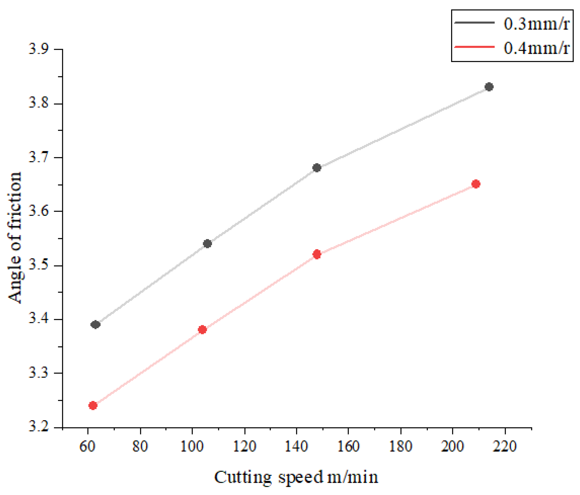
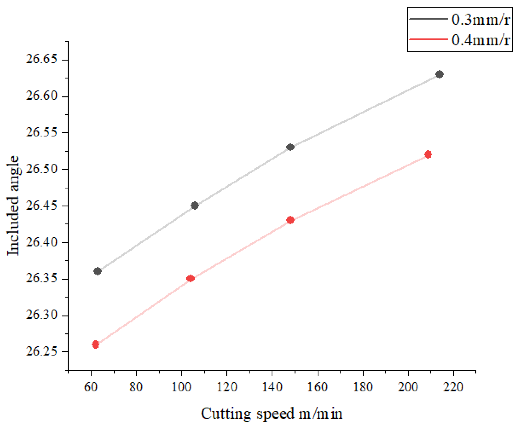
The friction angle is calculated as $\lambda =\theta +\alpha -\phi$. According to Oxley’s theory, the shear angle and the included angle satisfy the following relationship:

$$\tan \theta =1+2(\frac{\pi }{4}-\phi )-C_0$$

(11)

The modified strain rate constant $C_0$ [17] takes into account the effect of material strain and is expressed as follows:

$$C_0=C_{0xley}n\frac{B{\epsilon }_{AB}^n}{A+B{\epsilon }_{AB}^n}$$

(12)

where $C_{Oxley}$ is the length–width ratio of the shear band; A, B, and n are Johnson–Cook constitutive parameters, respectively.

According to the Boothroyd temperature model [18], the average temperature is expressed as follows:

$$T_{AB}=T_r+\eta \frac{(1-\beta )F_s{V}_s}{{\rho }_w{C}_{w}V{t}_{1}w\sin \phi }$$

(13)

where $T_r$ is the workpiece temperature, $\eta$ is the average temperature coefficient, 0.9 [19]; ${\rho }_{{}_w}$ is the material density; $C_w$ is the specific heat capacity; and $\beta$ is the heat distribution coefficient [17].

$$\beta =\{\begin{array}{c}0.5-0.35\lg \left(R_0\tan \phi \right)\begin{array}{cc}& 0.04\le R_0\tan \phi \le 10\end{array}\\ 0.3-0.15\lg \left(R_0\tan \phi \right)\begin{array}{cc}& R_0\tan \phi \text{>}10\end{array}\end{array}$$

(14)

$$R_0=\frac{{\rho }_w{C}_{w}V{t}_1}{K_w}$$

(15)

where $K_w$ is the thermal conductivity.

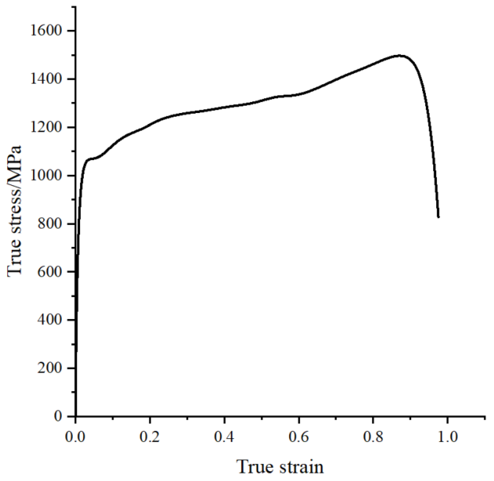
In high-speed cutting, the material undergoes a process of large strain, with a high strain rate and high temperature. S32760 duplex stainless steel shows an obvious viscous effect with a strain rate above 10⁴ s⁻¹ [20]. Therefore, in order to consider the viscous behavior of this material, in the Oxley theoretical model, the S32760 two-phase constitutive model considering the viscous effect should be used to predict the flow stress in the shear zone.

The MTS constitutive model is improved by also considering the viscous effect. The equation is divided into three parts as follows:

$$\sigma ={\sigma }_a+f(\dot{\epsilon },T){\sigma }_{th}+{\sigma }_c$$

(16)

where ${\sigma }_a$ is the non-thermal stress value; $f(\dot{\epsilon },T)$ is the influence factor of the reaction strain rate and the temperature effect; ${\sigma }_{th}$ is the thermal stress value; and ${\sigma }_c$ is the stickiness effect.

Due to the dual-phase property of the material, the three stresses of the ferrite and austenite phases need to be calculated separately, and the weighted sum is given by

$$\sigma =l_1{\sigma }_1+l_2{\sigma }_2$$

(17)

where $l_1$ is the proportion of the ferrite phase; $l_2$ is the proportion of the austenite phase; ${\sigma }_1$ is the stress in the ferrite phase; and ${\sigma }_2$ is the stress in the austenite phase.

The non-thermal stress value is independent of the effect of strain rate and temperature change and is only affected by changes in strain. Since the influence of the strain rate and temperature on the ferrite’s work-hardening behavior can be neglected, the flow stress increased by the work-hardening behavior of ferrite is included in the ferrite’s non-thermal stress value. The non-thermal stress values in the constitutive equations of ferrite and austenite can be written as follows:

$${\sigma }_{a1}={\sigma }_{i1}+m_1{d}_1^{-\frac{1}{2}}+K_1{\epsilon }^{n_1}$$

(18)

$${\sigma }_{a2}={\sigma }_{i2}+m_2{d}_2^{-\frac{1}{2}}$$

(19)

where ${\sigma }_{i1}$ and ${\sigma }_{i2}$ are the total stress of dislocation movement in ferrite and austenite, respectively; $m_1$ and $m_2$ are constants representing grain boundary strength of ferrite and austenite, respectively; $d_1$ and $d_2$ are the grain size of ferrite and austenite, respectively; $K_1$ is the ferrite hardening coefficient; $\epsilon$ is the true strain; $n_1$ is the ferrite strain sensitivity index.

The expression of the influence factor is given as follows [21]:

$$f(\dot{\epsilon },T)={\left\{1-{\left[-\frac{kT}{G_0}\ln (\frac{\dot{\epsilon }}{{\dot{\epsilon }}_0})\right]}^{\frac{1}{q}}\right\}}^{\frac{1}{p}}$$

(20)

where $k$ is the Boltzmann constant; $T$ is the temperature; $G_0$ is the reference thermal activation energy; ${\dot{\epsilon }}_0$ is the reference strain rate; and $p,q$ are the barrier constants.

Since the thermal stress of the body-centered cubic structure is independent of the strain, the thermal stress value ${\sigma }_{th1}$ of the ferrite is equal to the ferrite saturation stress value. Therefore, following [21], we have

$${\sigma }_{th1}={\widehat{\sigma }}_{s1}{e}^{\frac{kT}{b^{3}E{a}_0}\ln \frac{\dot{\epsilon }}{{\dot{\epsilon }}_{s0}}}$$

(21)

where ${\widehat{\sigma }}_{s1}$ is the reference value of ferrite saturation threshold stress at T = 0 K; $b$ is the Burgers vector of dislocation; $E$ is the shear modulus of the material; and $a_0$ is a constant.

For austenite, the work-hardening rate is high. Therefore, the effect of strain rate and temperature needs to be considered in austenite strain hardening. Therefore, following [22],

$${\sigma }_{th2}=K_2{\epsilon }^{n_2}{\widehat{\sigma }}_{s2}{e}^{\frac{kT}{b^{3}E{a}_0}\ln \frac{\dot{\epsilon }}{{\dot{\epsilon }}_{s0}}}$$

(22)

where $K_2$ is the austenite strain-hardening coefficient; $n_2$ is the austenite strain sensitivity index; and ${\widehat{\sigma }}_{s2}$ is the reference value of austenitic saturation threshold stress at T = 0 K.

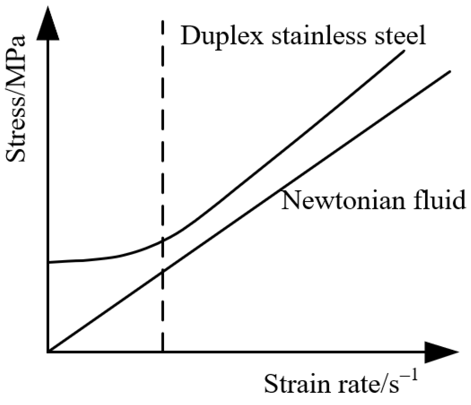
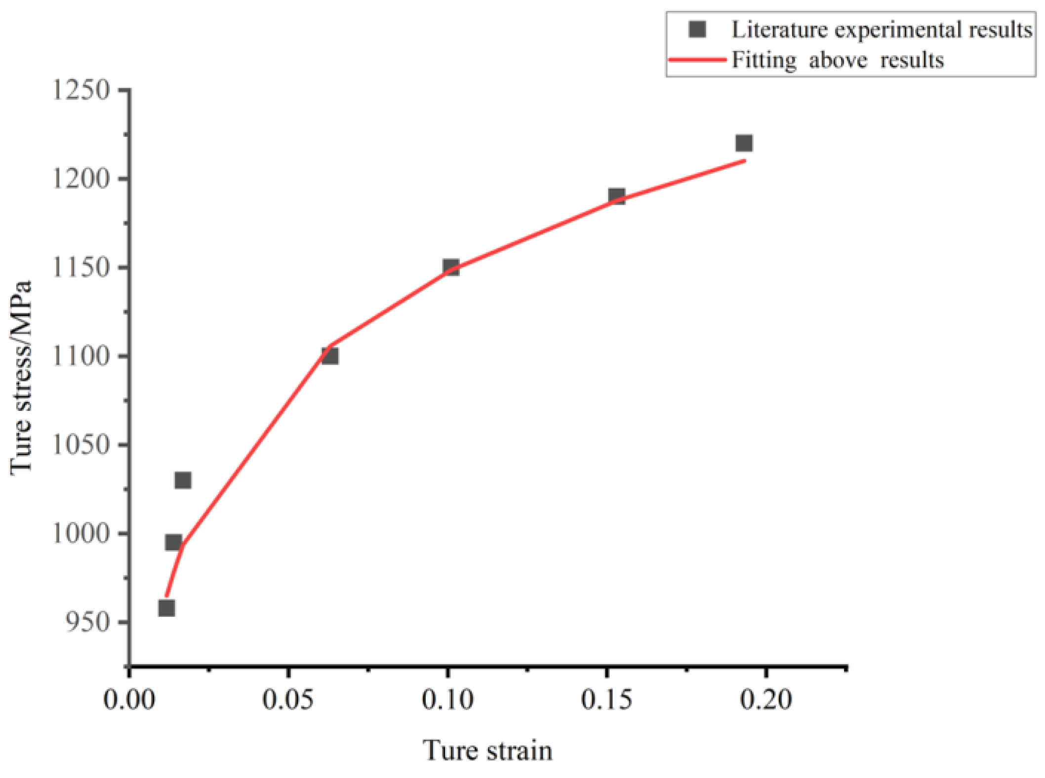
Kazban [23] studied the change in the flow stress of duplex stainless steel with the strain rate and found that the change in flow stress is similar to that of a Newtonian fluid after a certain strain rate value. The comparison of stress–strain rate relationship between duplex stainless steel and a Newtonian fluid is shown in Figure 2.

The viscous behavior of the material is related to the dislocation velocity. The higher the dislocation velocity, the more obvious the viscous effect of dislocation is and the more obvious the viscous effect of the material. The damping force of dislocation motion is given by Kuksin [24] as follows:

$$F_v={\mu }_d{v}_d$$

(23)

where ${\mu }_d$ is the viscous damping coefficient, and $v_d$ is the dislocation velocity.

The force required for dislocation motion is as follows:

$$F=\tau b$$

(24)

where $\tau$ is the shear stress on the dislocation plane, and b is the Burgers vector of the dislocation.

The dislocation inside the metal is caused by the stress generated by the external force. Orowan [25] first proposed the relationship between the plastic strain rate $\dot{\epsilon }$ and the average dislocation velocity as follows:

$$\dot{\epsilon }={\rho }_{d}b{v}_d$$

(25)

where ${\rho }_d$ is the dislocation density.

In the metal-cutting process, the dislocation velocity is approximately equal to the cutting speed. In the whole process from the beginning of the slip motion until dislocation, the force of the dislocation motion is balanced with the resistance that hinders the dislocation motion so as to ensure stability and a smooth cutting process. This equilibrium is expressed as follows:

$$F_v=F$$

(26)

According to Newton’s law of internal friction, the shear stress of a Newtonian fluid can be expressed as follows:

$$\tau =\mu \dot{\epsilon }$$

(27)

From this, the viscous effects of ferrite and austenite are:

$${\sigma }_{c1}=\frac{{\mu }_{d1}}{{\rho }_{d1}{b}_1{}^2}\dot{\epsilon }$$

(28)

$${\sigma }_{c2}=\frac{{\mu }_{d2}}{{\rho }_{d2}{b}_2{}^2}\dot{\epsilon }$$

(29)

$\overline{\sigma }=l_1({\sigma }_{i1}+m_1{d}_1^{-\frac{1}{2}})+l_2({\sigma }_{i2}+m_2{d}_2^{-\frac{1}{2}})$, $\overline{K}=l_1{K}_1$, ${\widehat{\sigma }}_{sh}=l_1{\widehat{\sigma }}_{s1}$, $\alpha =\frac{k}{b^{3}E{a}_0}$,$\beta =\frac{k}{G_0}$, $\overline{Y}=l_2{K}_2{\widehat{\sigma }}_{s2}$, $\mu =l_1\frac{{\mu }_{d1}}{{\rho }_{d1}{b}_1^2}+l_2\frac{{\mu }_{d2}}{{\rho }_{d2}{b}_2^2}$. The constitutive equation of S32760 duplex stainless steel is:

$$\sigma =\overline{\sigma }+\overline{K}{\epsilon }^{n_1}+(\overline{Y}{\epsilon }^{n_2}+{\widehat{\sigma }}_{sh}){\{1-{\left[-\beta T\ln \left(\frac{\dot{\epsilon }}{{\dot{\epsilon }}_0}\right)\right]}^{\frac{1}{q}}\}}^{\frac{1}{p}}{e}^{\alpha T\ln \frac{\dot{\epsilon }}{{\dot{\epsilon }}_{s0}}}+\mu \dot{\epsilon }$$

(30)

There are a total of 13 parameters that need to be determined experimentally, namely $\overline{\sigma }$, $\overline{K}$, $\overline{Y}$, ${\widehat{\sigma }}_{sh}$, $n_1$, $n_2$, $\alpha$, $\beta$, ${\dot{\epsilon }}_0$, ${\dot{\epsilon }}_{s0}$, $p$, $q$, and $\mu$.

According to the von Mises criterion, the flow stress at the shear surface AB is given as follows:

$${\sigma }_{AB}=\frac{1}{\sqrt{3}}\{\overline{\sigma }+\overline{K}{\epsilon }_{AB}^{n_1}+\left(\overline{Y}{\epsilon }_{AB}^{n_2}+{\widehat{\sigma }}_{sh}\right){\{1-{\left[-\beta T_{AB}\ln \left(\frac{{\dot{\epsilon }}_{AB}}{{\dot{\epsilon }}_0}\right)\right]}^{\frac{1}{q}}\}}^{\frac{1}{p}}{e}^{\alpha T_{AB}\ln \frac{{\dot{\epsilon }}_{AB}}{{\dot{\epsilon }}_{s0}}}+\mu \dot{\epsilon }\}$$

(31)

2.2. Tool–Chip Contact Surface Analysis

In the analysis of the second deformation zone, it is generally assumed that the thickness of the plastic deformation zone of the tool–chip interface is a constant, namely $\Delta S_2=\delta t_2$, where $\delta$ is the ratio of the thickness of the second deformation zone to the chip thickness. Therefore, the equivalent strain and equivalent strain rate of the tool–chip interface are determined as follows:

$${\epsilon }_{\mathrm{int}}=2{\epsilon }_{AB}+\frac{1}{\sqrt{3}}\cdot \frac{h_{tc}}{\delta t_2}$$

(32)

$${\dot{\epsilon }}_{\mathrm{int}}=\frac{1}{\sqrt{3}}\cdot \frac{V_c}{\delta t_2}$$

(33)

where $h_{tc}$ is the tool–chip contact length, which can be calculated using the torque balance formula on the shear plane.

$$h_{tc}=\frac{t_1\sin \theta }{\cos \lambda \sin \phi }\left(1+\frac{C_0}{3\tan \theta }\right)$$

(34)

The average temperature $T_{\mathrm{int}}$ of the tool–chip interface is expressed as follows:

$$T_{\mathrm{int}}=T_r+\Delta T_{SZ}+\psi \Delta T_M$$

(35)

$$\lg \left(\frac{\Delta T_M}{\Delta T_C}\right)=0.06-\delta \sqrt{\frac{R_0{t}_2}{t_1}}+0.5\lg \left(\frac{R_0{t}_2}{h_{tc}}\right)$$

(36)

$$\Delta T_C=\frac{F_f{V}_c}{{\rho }_{w}V{t}_{1}w{C}_w}$$

(37)

where $\psi$ is the correction factor taken as 0.6 [26]; $\Delta T_M$ is the maximum temperature rise in chips; $\Delta T_C$ is the average temperature rise in chips; and $\Delta T_{SZ}$ is the temperature rise of the first deformation zone.

According to the characteristics of flow stress at the shear zone, the flow stress at the tool–chip contact interface is predicted using the S32760 two-phase constitutive model considering the viscous effect.

$${\sigma }_{chip}=\frac{1}{\sqrt{3}}\{\overline{\sigma }+\overline{K}{\epsilon }_{\mathrm{int}}^{n_1}+\left(\overline{Y}{\epsilon }_{\mathrm{int}}^{n_2}+{\widehat{\sigma }}_{sh}\right){\{1-{\left[-\beta T_{\mathrm{int}}\ln \left(\frac{{\dot{\epsilon }}_{\mathrm{int}}}{{\dot{\epsilon }}_0}\right)\right]}^{\frac{1}{q}}\}}^{\frac{1}{p}}{e}^{\alpha T_{\mathrm{int}}\ln \frac{{\dot{\epsilon }}_{\mathrm{int}}}{{\dot{\epsilon }}_{s0}}}+\mu \dot{\epsilon }\}$$

(38)

2.3. Modeling of Force of Chip Formation

Since the shear angle of the shear zone $\phi$, the deformation coefficient of the shear zone $C_{Oxley}$, and the ratio of the thickness of the second deformation zone to the chip thickness $\delta$ vary with cutting conditions, material properties, and tool geometry, these three variables are iterated over in ranges of $\phi \in [5°,45°]$, $C_{Oxley}\in [2,10]$, and $\delta \in [0.005,0.2]$, respectively. The calculation will be terminated when the output satisfies three equilibrium conditions: (i) the stress balance at the tool–chip interface; (ii) the stress balance at the tool tip; and (iii) the minimum principle of the cutting force ($F_c$) [27].

Assuming that the tool–chip interface stress is uniformly distributed, the expressions of the tool–chip interface stress ${\tau }_{\mathrm{int}}$ and stress ${\sigma }_N$ at point B are given as follows:

$$\{\begin{array}{c}{\tau }_{\mathrm{int}}=\frac{F_f}{h_{tc}w}\\ {\sigma }_N=\frac{F_N}{h_{tc}w}\end{array}$$

(39)

The normal stress ${\sigma }_N^{\prime }$ at point B near the tip in Figure 1 can be obtained by combining the average shear flow stress of the shear plane given as follows:

$${\sigma }_N^{\prime }={\sigma }_{AB}(1+\frac{\pi }{2}-2\alpha -2C_0)$$

(40)

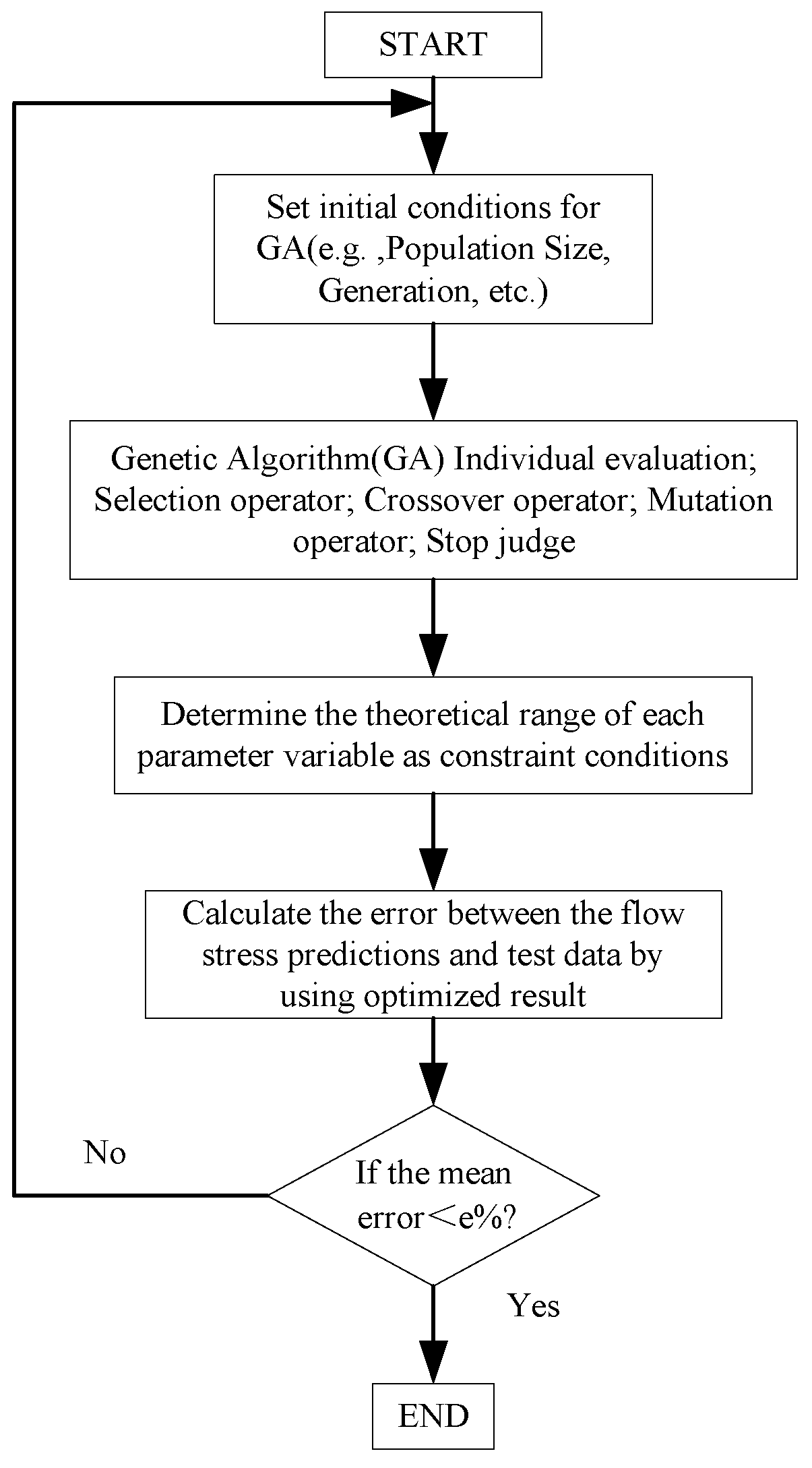
In the cutting-force prediction model, when solving the temperature of the shear zone, the flow stress of the shear zone is determined at a given initial temperature. The temperature of the shear surface is then updated according to the flow stress and replaced with the initial temperature to start a new calculation. This process is repeated until the difference between the initial temperature and the calculated temperature is less than 1 °C. When determining the tool–chip interface temperature, the sum of the increases in room temperature and the temperature of the first deformation zone is used as the initial temperature, and then the maximum increase in temperature and the average increase in the temperature of the chip are used as the temperature increment to determine the new chip temperature and replace it with the initial temperature to start a new calculation. The process is repeated until the difference between the initial temperature and the calculated temperature is less than 1 °C. The tangential stress of the tool–chip interface (${\tau }_{\mathrm{int}}$) and the flow stress of the tool–chip interface (${\sigma }_{chip}$) are compared, and the difference between the absolute values of the two is taken as the basis for judgment. The shear angle ($\phi$) takes the value of whichever has the smallest absolute value and is then used. The calculation of the various parameters in the shear zone is repeated. The normal stress of the tool tip (${\sigma }_N$), the normal stress of the B point near the tool tip (${\sigma }_N^{\prime }$), and the difference between the absolute values of the two are computed and used as the basis for judgment. The shear zone deformation coefficient ($C_{Oxley}$) takes the value of whichever has the smallest absolute value, and this shear zone deformation coefficient is then used. The calculation of the various parameters in the shear zone is then repeated and finally compared with the cutting force ($F_c$). The minimum value is selected to determine $\delta$.

Thus, considering different cutting conditions, material properties, and tool geometries using the chip formation force model, the calculation flowchart of the orthogonal cutting process is shown in Figure 3.

3. Parameter Optimization of the Constitutive Model

The challenge in developing the constitutive model is to identify the material parameters by applying the optimization algorithm to minimize the difference between the calculated value and the experimental value so that the constitutive model produces the optimal prediction result. Since there are many parameters to be identified, in this study, the multiobjective genetic algorithm was used for optimization.

3.1. Non-Thermal Stress Parameter Identification

In order to obtain the flow stress value of S32760 under a high strain rate, the two-phase constitutive equation of S32760 was fitted. The stress–strain curve of the material was obtained by employing the Hopkinson pressure bar equipment at a 10⁴ s⁻¹ strain rate and 500 °C. The Hopkinson pressure bar equipment used in the experiment was ARCHIMEDES ALT1000. The experimental material was a ϕ2 × 2 mm S32760 cylinder, as illustrated in Figure 4. The microstructure of S32760 duplex stainless steel under SEM observation is shown in Figure 5. The obtained stress–strain curve is shown in Figure 6. The chemical composition of S32760 duplex stainless steel is shown in

Table 1. Chemical composition of S32760 duplex stainless steel (mass fraction, %) [20].

C	Cr	Cu	C	Mn	Ni	P	S	W
0.03	25	0.75	3.5	1	7	0.03	0.01	0.75

[20]. The basic material parameters are shown in

Table 2. Basic material parameters of S32760 duplex stainless steel.

Density	Elastic Modulus	Poisson Ratio	Yield Strength	Tensile Strength	Microhardness of Austenite Phase	Microhardness of Ferrite Phase	Austenite Phase Ratio	Ferrite Phase Ratio
8000 kg/m3	204 GPa	0.3	596 MPa	964 MPa	317.5 HV0.05	351.3 HV0.05	46%	54%

.

Since the flow stress is not related to the temperature when the temperature is high enough, the experimental data obtained can be used for the least-square curve fitting. The curve-fitting results of non-thermal stress at the strain rate of 10⁴ s⁻¹ are shown in Figure 7. The three undetermined parameters in the non-thermal stress value obtained are as follows:

$$\overline{\sigma }=60,\overline{K}=1318,n_1=0.07997$$

3.2. Viscous Effect Parameter Selection

Since S32760 duplex stainless steel contains both BCC and FCC structures, the viscous effects of the two structures should be evaluated separately. The viscosity parameter of the BCC structure is $\mu =1.8\times {10}^{-3}$ [28], while the viscosity parameter of the FCC structure is $\mu =3.8\times {10}^{-3}$ [29]. Using ImageJ software V1.8.0.112 to analyze Figure 5, it can be seen that the proportion with the BCC structure was 54%, and the proportion with the FCC structure was 46%. Thus, the viscous effect parameter of S32760 duplex stainless steel was found to be $\mu =2.72\times {10}^{-3}$.

3.3. Optimal Selection of Thermal Stress Parameters

The parameters for the determination of thermal stress include $\overline{Y}$, ${\widehat{\sigma }}_{sh}$, $n_2$, $\alpha$, $\beta$, ${\dot{\epsilon }}_0$, ${\dot{\epsilon }}_{s0}$, $p$, and $q$. Since ${\dot{\epsilon }}_0$ and ${\dot{\epsilon }}_{s0}$ are not independent in parameter fitting, and both are included in the logarithmic function, the influence of changes in value on thermal stress is much smaller than that of the previous $\alpha$ and $\beta$. These values need to be predicted to better determine the parameters. S32760 duplex stainless steel has both BCC and FCC structures, and the constitutive equation of HCP metal can be regarded as a linear combination of BCC and FCC. Therefore, the reference strain rate of HCP metal can be used to determine the reference strain rate of S32760.

According to Nemat-Nasser [30], ${\dot{\epsilon }}_0={\dot{\gamma }}_0/f(\gamma ,T)$, where ${\dot{\gamma }}_0=b{l}_0{p}_w{w}_0$, $b=3\times {10}^{-10}$ m, $l_0=500$ b, $p_w={10}^{11}/$cm², $T=598$ k, and $\gamma =0.25$, and using these values, ${\dot{\epsilon }}_0=3\times {10}^9$ s⁻¹. Since the value of ${\dot{\epsilon }}_{s0}$ is generally two orders of magnitude larger than that of ${\dot{\epsilon }}_0$, ${\dot{\epsilon }}_{s0}=1\times {10}^{11}$ s⁻¹.

After determining ${\dot{\epsilon }}_0$ and ${\dot{\epsilon }}_{s0}$, the remaining parameters can be solved using the method of reverse identification.

The purpose of solving parameters is to find a set of material parameters that correlate with the physical meaning so that the curve solved using the constitutive equation is as consistent as possible with the curve obtained through experimentation. The objective function is defined using the principle of the least-square method. The sum of the squares of the difference between the stress value calculated using the constitutive equation and the stress value measured through experimentation is taken as the objective function so that the objective function is as small as possible. The objective function can be expressed as follows:

$$F(x)={\displaystyle \sum {}_{i=1}^N{(Y_i(x)-Y_i^{*})}^2}$$

(41)

where $x=[x_1,x_2,\dots ,x_m]$ is the parameter to be optimized, N is the number of points taken, $Y_i$ is the value calculated at the i-th point, and $Y_i{}^{*}$ is the value measured using the i-th point experiment.

In this study, the MATLAB program was used to optimize the computation of the objective function. The flowchart of the constitutive model parameter optimization program is shown in Figure 8. In addition, in order to ensure the accuracy of the calculation results, it was necessary to determine the theoretical range of each parameter.

The remaining unknown parameters were grouped as follows:

• Determination of $\overline{Y}$ and ${\widehat{\sigma }}_{sh}$: Based on the work carried out by Nemat-Nasser et al. [30], the terms $1560\times f(\epsilon ,T)$ and ${\widehat{\sigma }}_{sh}+\overline{Y}{\epsilon }^{n_2}$ in Equation (8) belong to the same category, and thereby, this equation could be effectively employed as a basis for determining the ranges of $\overline{Y}$ and ${\widehat{\sigma }}_{sh}$. The median value of the range of ${\widehat{\sigma }}_{sh}$ was 1560, and it was extended to both ends to determine ${\widehat{\sigma }}_{sh}\in [1000,2000]$. The range of temperature T was set as 77–998 K, while strain was maintained in the range of 0–0.6. Thus, we estimated $\overline{Y}\in [1500,3500]$.
• Determination of $\alpha$ and $\beta$: The Boltzmann constant was $k=1.3806505\times {10}^{-23}$ J/K and for S32760 stainless steel, $b=3\times {10}^{-10}$ m, shear modulus $E=159.2$ GPa, $a_0\in (0.2,2)$ [30,31], and $\alpha =k/(b^{3}E{a}_0)$. The value $\alpha \in (1.6\times {10}^{-6},1.6\times {10}^{-5})$ was estimated, and the upper and lower bounds of this range were expanded to a certain extent, taking the theoretically allowable maximum change range $(1\times {10}^{-6},1\times {10}^{-4})$. Since $\alpha$ and $\beta$ belong to the same order of magnitude, it can be considered that $\alpha$ and $\beta$ have the same range.
• Determination of $n_2$: It is generally believed that for most FCC metals, $n_2$ is 0.5, and for individual metals, there may be a small variation around 0.5. On this basis, for S32760, we considered the maximum variation range allowed by this theory, i.e., (0,1].
• Determination of p and q: p and q are a pair of correlation constants that determine the shape of the barrier, and the intervals 0 < p ≤ 1, 1 ≤ q < 2 [32], are generally taken for single crystals. Several typical (p, q) values such as (2/3, 1), which represents a rectangular barrier; (1/2, 2), which specifies a hyperbolic barrier; and (1, 2), which denotes a sinusoidal barrier, were adopted. For most metals, (p, q) could be considered as (2/3, 1), (2/3, 2), (3/4, 4/3), and (1, 1), i.e., a transition between rectangular and sinusoidal shapes. Although the values of p and q introduced above are applicable to single crystals, they could also be exploited for S32760 since the p and q parameters in the constitutive model are the mean values of the same variables in the constitutive models of the BCC and FCC structures.

The range of parameters in the constitutive model determined above is the parameter range of the genetic algorithm. In this paper, a genetic algorithm was used to optimize the parameters, and a set of constitutive model parameters were calculated using the GA Optimization Toolbox. The thermal stress parameters of the S32760 constitutive model are shown in

Table 3. Thermal stress parameters of S32760 constitutive model.

Undetermined Constitutive Parameters	The Actual Estimation Range	Definite Value	Unit
$\overline{Y}$	[1500, 3500]	3149.06	Mpa
$n_2$	(0,1)	0.2680	/
${\widehat{\sigma }}_{sh}$	[1000, 2000]	1880.62	Mpa
$\alpha$	(10−6, 10−4)	0.00002298	1/K
$\beta$	(10−6, 10−4)	0.00009213	1/K
q	[1, 2]	1.6809	/
p	(0, 1)	0.0191	/

.

Therefore, a set of initial values of the constitutive parameters of S32760 duplex stainless steel were obtained. The experimental data for the orthogonal cutting process were then used as a reference to reverse identification on the thermal stress value so that the constitutive parameters were continuously corrected until the difference between the experimental value and the simulated value was minimized.

According to the constitutive parameters obtained in Table 3, the developed S32760 constitutive model is given as follows:

$$\begin{array}{l}\sigma =60+1318{\epsilon }^{0.07997}+\\ (3149.06{\epsilon }^{0.268}+1880.62){\left\{1-{\left[-0.00009213T\ln (\frac{\dot{\epsilon }}{3\times {10}^9})\right]}^{\frac{1}{1.6809}}\right\}}^{\frac{1}{0.0191}}{e}^{0.00002298T\ln (\frac{\dot{\epsilon }}{{10}^{11}})}+0.00272\dot{\epsilon }\end{array}$$

(42)

4. Parameter Reverse Identification Combined with Cutting Theory

4.1. Orthogonal Cutting Experiment

A test platform was built for orthogonal cutting, and the reliability of the cutting-force analysis model for the orthogonal cutting of S32760 duplex stainless steel was verified. Figure 9 is the orthogonal cutting test platform. The bar size was ϕ70 mm × 130 mm. A three-jaw fixture was used to clamp the bar stock. Rough turning with a 1 mm depth of cut was carried out, followed by a 3 mm width of grooving. Multiple grooves with a groove depth of 3 mm and groove spacing of 2 mm were generated. The tool model was MGGN300-V DH8532. The rake and back angles were set as 18° and 8°, respectively, and the blade inclination angle was set equal to 0°. The edge radius was 0.02 mm, as demonstrated in Figure 10. The toolholder model was MGEHR2525-3. The orthogonal cutting experiment was carried out on a CKA6150 machine tool produced by Dalian Machine Tool Factory.

The instrument used for measuring the cutting force was KISTLER piezoelectric dynamometer 9139AA. The dynamometer can measure the cutting force in three directions during the cutting process. In order to ensure the accuracy of the measurement results, each group of experiments was repeated three times, and the mean value was taken. In order to verify the accuracy of the cutting-force prediction model, the cutting parameters of orthogonal cutting experiments were determined, which are shown in

Table 4. The cutting parameters for the right-angle cutting experiment.

Test Number	Cutting Speed m/min	Feed Rate mm/r	Cutting Depth
1	63	0.3	3 mm
2	106	0.3	3 mm
3	148	0.3	3 mm
4	214	0.3	3 mm
5	62	0.4	3 mm
6	104	0.4	3 mm
7	148	0.4	3 mm
8	209	0.4	3 mm
9	63	0.35	3 mm
10	106	0.35	3 mm
11	148	0.35	3 mm
12	214	0.35	3 mm

. The first eight sets of experimental data were used to correct the constitutive parameters, and the last four sets of data were used to verify the accuracy of the constitutive model.

The cutting force’s scatter plot is demonstrated in Figure 11. The cutting-force values obtained using the orthogonal cutting experiment are shown in

Table 5. Cutting force of orthogonal cutting experiment.

Test Number	${\mathit{F}}_{\mathit{c}}/\mathbf{N}$	${\mathit{F}}_{\mathit{t}}/\mathbf{N}$
1	747	190
2	753	193
3	760	201
4	765	210
5	976	249
6	982	257
7	989	263
8	993	270
9	859	222
10	870	225
11	877	237
12	885	242

.

4.2. Parameter Correction

The parameters of the equal shear zone model that were required for S32760 orthogonal cutting are shown in

Table 6. The parameters of the equal shear zone model required for S32760 orthogonal cutting.

Parameter	Numerical Value	Unit
${\rho }_w$	8000	Kg/m3
$C_w$	434.8	J/Kg·°C
$K_w$	17.6	W/m·°C
A	596	MPa
B	964	MPa
n	0.138	/

.

It is observed that the strain rate increased with an increase in the cutting speed. When the strain rate increased to more than 10⁴ s⁻¹, the dislocation slip velocity was controlled using the viscous resistance of dislocation, and the cutting process showed a viscous flow process similar to that of a fluid. The variation in the strain rate relative to the cutting speed is shown in Figure 12.

From Equations (1), (2), and (5), the relationship between the flow stress and the cutting force is as follows:

$$\{\begin{array}{c}{\sigma }_{AB}=F_c\frac{\sin \phi \cos \theta }{\cos (\lambda -\alpha )t_{1}w}\\ {\sigma }_{AB}=F_t\frac{\sin \phi \cos \theta }{\sin (\lambda -\alpha )t_{1}w}\end{array}$$

(43)

The shear angle $\phi$, friction angle $\lambda$, and the included angle $\theta$ were solved iteratively using the equal shear zone model. The parameters listed in Table 4 and Table 6 were input into the equal shear zone model, and the predicted values of the equal shear zone model were obtained, which are shown in

Table 7. Predicted values of equal shear zone model.

Test Number	Strain	Strain Rate/s−1	$\mathbf{Angle}\mathbf{of}\mathbf{Shear}\mathit{\phi }$ /°	$\mathbf{Angle}\mathbf{of}\mathbf{Friction}\mathit{\lambda }$ /°	$\mathbf{Included}\mathbf{Angle}\mathit{\theta }$ /°
1	0.4548	10,811	40.97	3.39	26.36
2	0.4551	18,161	40.91	3.54	26.45
3	0.4555	25,317	40.85	3.68	26.53
4	0.4558	36,549	40.79	3.83	26.63
5	0.4545	7992	41.02	3.24	26.26
6	0.4548	13,385	40.95	3.38	26.35
7	0.4551	19,018	40.90	3.52	26.43
8	0.4555	26,814	40.83	3.65	26.52

.

The effects of the cutting speed on the shear angle, friction angle, and angle was analyzed, and the results are presented in Figure 13, Figure 14 and Figure 15. It can be seen from Figure 13 that the shear angle decreased with an increase in the cutting speed. The plotted results in Figure 14 indicate that the friction angle increased with the increase in the cutting speed. Figure 15 shows that the included angle increased with the increase in the cutting speed.

Therefore, from the relationship between the flow stress and the cutting component, the constitutive parameters were identified using the principle of the least-square method. The sum of the squares of the difference between the flow stress value calculated using the constitutive equation, and the flow stress value obtained using the cutting component was taken as the objective function so that the objective function would be as small as possible. The objective function is expressed as follows:

$$P(y)={\displaystyle \sum {}_{i=1}^N{({\sigma }_i(y)-{\sigma }_{AB})}^2}$$

(44)

where $y=[\overline{Y},n_2,{\widehat{\sigma }}_{sh},\alpha ,\beta ,p,q]$ is the parameter to be optimized, N is the number of points taken, ${\sigma }_i$ is the value calculated using the constitutive equation at the i-th point, and ${\sigma }_{AB}$ is the value calculated using the cutting component at the i-th point.

The MATLAB program was used to optimize the calculation. The flowchart of the constitutive model parameters is shown in Figure 16, and the theoretical range of the parameters is the same as that in Table 3.

The modified equation is:

$$\begin{array}{l}\sigma =60+1318{\epsilon }^{0.07997}+\\ (3217.76{\epsilon }^{0.3036}+1325.53){\left\{1-{\left[-0.00005918T\ln (\frac{\dot{\epsilon }}{3\times {10}^9})\right]}^{\frac{1}{1.3527}}\right\}}^{\frac{1}{0.0189}}{e}^{0.00002159T\ln (\frac{\dot{\epsilon }}{{10}^{11}})}+0.00272\dot{\epsilon }\end{array}$$

(45)

4.3. Model Validation

The comparison between the cutting force of the orthogonal cutting test and the cutting force predicted using the model is shown in

Table 8. Comparison of experimental cutting force and predicted cutting force.

Test Number	$\mathbf{Experiment}{\mathit{F}}_{\mathit{c}}/\mathbf{N}$	$\mathbf{Experiment}{\mathit{F}}_{\mathit{t}}/\mathbf{N}$	$\mathbf{Prediction}{\mathit{F}}_{\mathit{c}}/\mathbf{N}$	$\mathbf{Prediction}{\mathit{F}}_{\mathit{t}}/\mathbf{N}$
9	859	222	879	230
10	870	225	893	231
11	877	237	906	232
12	885	242	926	235

.

The experimentally obtained cutting force and the predicted cutting force at a feed rate of 0.35 mm/r are shown in Figure 17. The analysis shows that the maximum prediction error of the cutting force $F_c$ was 4.6%, the minimum prediction error was 2.6%, and the average prediction error was 3.3% when the feed rate was 0.35 mm/r. The maximum prediction error of the cutting force $F_t$ was 3.6%, the minimum prediction error was 2.1%, and the average prediction error was 2.8%. It can be seen that the constitutive model developed in this paper is quite accurate in predicting the cutting force. The analysis of the relationship between the cutting speed and the cutting force revealed that the cutting force increased with the increase in cutting speed.

5. Conclusions

Based on the experimental design, mixing rule, and equal shear zone modeling of the orthogonal cutting process, an inverse identification method was proposed to determine the MTS constitutive parameters of S32760 duplex stainless steel. The viscosity behavior of the austenite and ferrite phases in duplex stainless steel was analyzed. It was found that the viscosity of the austenite phase was greater than that of the ferrite phase, and the viscosity of the austenite phase could reach twice that of the ferrite phase.

The strain, strain rate, and friction angle increased with an increase in the cutting speed; however, the shear angle decreased. The strain rate had no effect on non-thermal stress. The non-thermal stress value was independent of the strain rate and temperature change and was only affected by changes in strain. The strain rate had a logarithmic effect on thermal stress, but its influence was small. By contrast, the strain rate had a linear effect on the viscous effect, and its influence was significant.

The constitutive model modified using the reverse identification method was used in the equal shear zone model of orthogonal cutting to predict the cutting force, and the results were compared with the cutting force values obtained through experimentation. The analysis showed that the cutting force increased with an increase in the cutting speed, and the average error in the prediction of $F_c$ and $F_t$ was less than 4%. The proposed inverse recognition algorithm and MTS constitutive model effectively improved the reliability and accuracy of the simulation results.